SHM⁺⁺: A Refinement of the Standard Halo Model for Dark Matter Searches

Abstract

Predicting signals in experiments to directly detect dark matter (DM) requires a form for the local DM velocity distribution. Hitherto, the standard halo model (SHM), in which velocities are isotropic and follow a truncated Gaussian law, has performed this job. New data, however, suggest that a substantial fraction of our stellar halo lies in a strongly radially anisotropic population, the ‘Gaia Sausage’. Inspired by this recent discovery, we introduce an updated DM halo model, the SHM⁺⁺, which includes a ‘Sausage’ component, thus better describing the known features of our galaxy. The SHM⁺⁺ is a simple analytic model with five parameters: the circular speed, local escape speed and local DM density, which we update to be consistent with the latest data, and two new parameters: the anisotropy and the density of DM in the Sausage. The impact of the SHM⁺⁺ on signal models for WIMPs and axions is rather modest since the multiple changes and updates have competing effects. In particular, this means that the older exclusion limits derived for WIMPS are still reasonably accurate. However, changes do occur for directional detectors, which have sensitivity to the full three-dimensional velocity distribution.

I Introduction

Historically, analyses of direct searches for dark matter (DM) have constructed signal models based upon the Gaussian distribution of velocities found in the standard halo model (SHM). This is inspired by isothermal spheres, which have asymptotically flat rotation curves. They are the only exact, self-gravitating systems with Gaussian velocity distributions Chandrasekhar (1939). Of course, it has long been known that the SHM is an idealisation Evans and An (2006); Vogelsberger et al. (2009); Zemp et al. (2009); Kuhlen et al. (2010); Mao et al. (2014), but it provides an excellent trade-off between simplicity and realism. The effects of non-Maxwellian speed distributions Kuhlen et al. (2010); Ling et al. (2010); Mao et al. (2013), triaxiality Evans et al. (2000), velocity anisotropy Fairbairn and Schwetz (2009); Knirck et al. (2018); March-Russell et al. (2009); Bozorgnia et al. (2013a); Fornasa and Green (2014), streams Savage et al. (2006); Lee and Peter (2012); Purcell et al. (2012); O’Hare and Green (2014, 2017); Foster et al. (2018), and other dark substructures Bruch et al. (2009); Lisanti et al. (2011); Lisanti and Spergel (2012); Billard et al. (2013); Kavanagh and O’Hare (2016) have all received attention using simple elaborations of the SHM. These studies were speculative and theoretically motivated given that in the past there was sparse knowledge about the true DM velocity distribution. While it is possible, and in some cases advisable, to derive exclusion limits on DM particle physics without any astrophysical assumptions, e.g. Refs. Fox et al. (2011); McCabe (2011); Frandsen et al. (2012); Gondolo and Gelmini (2012); Herrero-Garcia et al. (2012); Frandsen et al. (2013); Bozorgnia et al. (2013b); Feldstein and Kahlhoefer (2014a); Fox et al. (2014); Feldstein and Kahlhoefer (2014b); Anderson et al. (2015); Gelmini et al. (2016); Kahlhoefer and Wild (2016); Gondolo and Scopel (2017); Gelmini et al. (2017); Ibarra and Rappelt (2017); Fowlie (2017), this often comes at the cost of greater complexity and less overall constraining power.

The arrival of the second data release from the Gaia satellite has been transformational for our understanding of the structure of the Galaxy Gaia Collaboration et al. (2018). The shape of the stellar halo, the local DM density, the local circular speed, the escape velocity and the history of accretion have all been the subject of sometimes radical revision in the wake of the new and abundant data Lancaster et al. (2018a); Wegg et al. (2018); Belokurov et al. (2018). Our understanding of the DM halo has not been left unscathed by the Gaia Revolution, and the time is ripe to put forward a new standard halo model, SHM⁺⁺, that represents our current knowledge, yet rivals the SHM in simplicity and realism.

The most substantial change brought about by Gaia data is that the local stellar halo is now known to have two components Carollo et al. (2007); Myeong et al. (2018a); Belokurov et al. (2018); Mackereth et al. (2018). The more metal-poor stars form a weakly rotating structure that is almost spherical (with axis ratio $q\approx 0.9$). This is likely the residue of many ancient accretions from low mass dwarf galaxies in random directions so that the net angular momentum of the accumulated material is almost zero. The more metal-rich stars form a flattened ($q\approx 0.6$), highly radially anisotropic structure. This is the “Gaia Sausage”. It was created by the more recent accretion of a large dwarf galaxy of mass $\approx 10^{10}-10^{11}\,\textrm{M}_{\odot}$ around 8 to 10 billion years ago (Belokurov et al., 2018; Helmi et al., 2018; Kruijssen et al., 2018), which will have been accompanied by a corresponding avalanche of DM.

Given what we now know about the stellar halo, it is natural to expect that the local DM halo also has a bimodal structure, made up from a rounder, isotropic component with velocity distribution $f_{\rm R}$ and a radially anisotropic Sausage component $f_{\rm S}$. In ref. (Necib et al., 2018), the velocity distributions of these two components were inferred from the velocities of stellar populations. Here, we provide simple analytic velocity distributions that capture the generic features of both components. The fraction of the local DM in the Sausage $\eta$ is not well known, though we will argue that it lies between 10% and 30%. The velocity anisotropy of DM in the Sausage $\beta$ is also not known, but the stellar and globular cluster populations associated with the Sausage are all extremely eccentric and so must be the DM.

In Section II, we discuss the shortcomings of the SHM in the light of recent advances in our knowledge of Galactic structure. Section III introduces the SHM⁺⁺, which acknowledges explicitly the bimodal structure of the Galaxy’s dark halo. We also take the opportunity to update the Galactic constants in the SHM⁺⁺, as the familiar choices for the SHM represent the state of knowledge that is now over a decade or more old. In Section IV, we discuss how our model compares with other complementary strategies for determining the local velocity distribution of DM. Then, Section V discusses the implications for a range of WIMP and axion direct detection experiments. We sum up in Section VI.

II The SHM: A Critical Discussion

At large radii the rotation curve of the Milky Way is flat to a good approximation (Sofue et al., 2009). The family of isothermal spheres (of which the most familiar example is the singular isothermal sphere) provide the simplest spherical models with asymptotically flat rotation curves Binney and Tremaine (2007). These models all have Gaussian velocity distributions.

The SHM was introduced into astroparticle physics over thirty years ago (Drukier et al., 1986). It models a smooth round dark halo. The velocity distribution for DM is a Gaussian in the Galactic frame, namely

$$f_{\rm R}(\mathbf{v})=\frac{1}{(2\pi\sigma_{v}^{2})^{3/2}N_{\mathrm{R,esc}}}\,\exp\left(-\frac{|\mathbf{v}|^{2}}{2\sigma_{v}^{2}}\right)\,$$

$$\times\Theta(v_{\mathrm{esc}}-|\mathbf{v}|)\,,$$ (1)

where $\sigma_{v}$ is the isotropic velocity dispersion of the DM and $v_{0}=\sqrt{2}\sigma_{v}$ is the value of the asymptotically flat rotation curve. The isothermal spheres all have infinite extent, whereas Galaxy halos are finite. This is achieved in the SHM by truncating the velocity distribution at the escape speed $v_{\mathrm{esc}}$, using the Heaviside function $\Theta$. The constant $N_{\mathrm{R,esc}}$ is used to renormalize the velocity distribution after truncation,

$$N_{\mathrm{R,esc}}=\mathrm{erf}\left(\frac{v_{\mathrm{esc}}}{\sqrt{2}\sigma_{v}}\right)-\sqrt{\frac{2}{\pi}}\frac{v_{\mathrm{esc}}}{\sigma_{v}}\exp\left(-\frac{v_{\mathrm{esc}}^{2}}{2\sigma_{v}^{2}}\right)\,.$$ (2)

Hence to describe the velocity distribution of DM in the galactic frame under the SHM we only need to prescribe two parameters, $v_{0}$ and $v_{\mathrm{esc}}$. The value of $v_{0}$ is usually taken as equivalent to the velocity of the Local Standard of Rest (or the circular velocity at the Solar position). The assumed value of $v_{\mathrm{esc}}$ has also typically been inspired by various astronomical determinations. The standard values for these quantities in the SHM are listed in Table 1. These values are, however, now somewhat out of date having undergone significant revision in recent years. One motivation for updating the SHM is to incorporate the more recent values for these parameters.

SHM	Local DM density	$\rho_{0}$	$0.3\,\mathrm{GeV}\,\mathrm{cm}^{-3}$
	Circular rotation speed	$v_{0}$	$220\textrm{ km s}^{-1}$
	Escape speed	$v_{\mathrm{esc}}$	$544\textrm{ km s}^{-1}$
	Velocity distribution	$f_{\rm R}(\mathbf{v})$	Eq. (II)
SHM++	Local DM density	$\rho_{0}$	$0.55\pm 0.17\textrm{ GeV cm}^{-3}$
	Circular rotation speed	$v_{0}$	$233\pm 3\textrm{ km s}^{-1}$
	Escape speed	$v_{\mathrm{esc}}$	$528^{+24}_{-25}\textrm{ km s}^{-1}$
	Sausage anisotropy	$\beta$	$0.9\pm 0.05$
	Sausage fraction	$\eta$	$0.2\pm 0.1$
	Velocity distribution	$f(\mathbf{v})$	Eq. (3)

Table 1: The astrophysical parameters and functions defining the SHM and the SHM⁺⁺. We include a recommendation for the uncertainty on each parameter for analyses that incorporate astrophysical uncertainties. While the uncertainties associated with $\rho_{0}$, $v_{0}$ and $v_{\mathrm{esc}}$ are based on direct measurements, the uncertainties associated with $\beta$ and $\eta$ are less certain. We refer the reader to the discussion in Section IIIA and IIIB respectively for more details.

The SHM has some successful features that we want to maintain. Current theories of galaxy formation in the cold dark matter paradigm envisage the build-up of DM halos through accretion and merger. In the inner halo (where the Sun is located), the distribution of DM particles extrapolated via sub-grid methods in high resolution dissipationless simulations like Aquarius is rather smooth (Vogelsberger and White, 2011), so a smooth velocity distribution is a good assumption. Furthermore, recent hydrodynamic simulations Bozorgnia et al. (2016); Kelso et al. (2016); Sloane et al. (2016); Lentz et al. (2017) have recovered speed distributions for DM that are better approximated by Maxwellian-distributions than their earlier N-body counterparts Hansen et al. (2006); Vogelsberger et al. (2009); Kuhlen et al. (2010); Ling et al. (2010); Mao et al. (2013, 2014). In this light, the assumption in the SHM of a Gaussian velocity distribution is surprisingly accurate.

There is, however, a significant shortcoming to the SHM. Gaia data has provided significant new information about the stellar and dark halo of our own Galaxy. The halo stars in velocity space exhibit abrupt changes at a metallicity of [Fe/H] $\approx-1.7$ (Myeong et al., 2018a). The metal-poor population is isotropic, has prograde rotation $(\langle v_{\phi}\rangle\approx 50$ km s^-1), mild radial anisotropy and a roundish morphology (with axis ratio $q\approx 0.9$). In contrast, the metal-rich stellar population has almost no net rotation, is very radially anisotropic and highly flattened with axis ratio $q\approx 0.6-0.7$.

The velocity structure of the metal-rich population forms an elongated shape in velocity space, the so-called “Gaia Sausage” (Belokurov et al., 2018; Myeong et al., 2018b). It is believed to be caused by a substantial recent merger (Belokurov et al., 2018; Helmi et al., 2018; Kruijssen et al., 2018). The “Sausage Galaxy” must have collided almost head-on with the nascent Milky Way to provide the abundance of radially anisotropic stars. Even if its orbital plane was originally inclined, dynamical friction dragged the satellite down into the Galactic plane. Similarly, though its original orbit may only have been moderately eccentric, the stripping process created tidal tails that enforced radialisation of the orbit (Amorisco, 2017), giving the residue of highly eccentric stars in the Gaia Sausage. Therefore, the $\sim 10^{10}-10^{11}\,\textrm{M}_{\odot}$ of DM in the Sausage Galaxy (Belokurov et al., 2018; Myeong et al., 2018b) will have been continuously stripped over a swathe of Galactocentric radii, as the satellite sank and disintegrated under the combined effects of dynamical friction and radialisation.

The smooth round halo of the SHM cannot account for the highly radially anisotropic DM associated with the Gaia Sausage. The SHM must therefore be extended to include a DM component with the radially anisotropic kinematics that arise from the Sausage Galaxy merger. Before introducing our refinements in Section III, we review the remaining ingredients of the SHM to discuss their validity.

II.1 Sphericity

The stellar halo is clearly irregular as viewed in maps of resolved halo stars Belokurov et al. (2006). It comprises a hotchpotch of shells and streams, many of which are associated with the Gaia Sausage (e.g. the Virgo Overdensity and the Hercules-Aquila Cloud Simion et al. (2018)). However, analyses of the kinematic data from Gaia strongly suggest that the dark halo is a smoother and rounder super-structure. Despite the abundant substructure, the velocity ellipsoid of the stellar halo is closely aligned in spherical polar coordinates (Evans et al., 2016; Wegg et al., 2018). This is a natural consequence of the gravitational potential – and hence the DM distribution – being close to spherical (Smith et al., 2009; An and Evans, 2016). Prior to data from Gaia, there was a long-standing discrepancy regarding the dark halo shape. Analyses of the kinematics of streams preferred almost spherical or very weakly oblate shapes (Koposov et al., 2010; Bowden et al., 2015). In contrast, Jeans analyses of the kinematics of halo stars, which are subject to substantial degeneracies between the stellar density, the velocity anisotropy and the DM density, gave shapes varying from strongly oblate to prolate (Loebman et al., 2014; Bowden et al., 2016). Reassuringly, the most recent Jeans analyses of the kinematics of the stellar halo components with Gaia data release 2 (DR2) RR Lyraes find that the DM distribution is nearly spherical (Wegg et al., 2018), at least in the innermost 15 kpc. This already suggests that the DM associated with the Gaia Sausage is subdominant. The DM halo must be a smoother and rounder structure than the stellar halo. Therefore, the assumption of near-sphericity in the potential that underlies the SHM continues to be supported by the data.

II.2 Circular Velocity at the Sun

The angular velocity of the Sun, derived from the Very-long-baseline interferometry proper motion of Sgr A^⋆ assuming it is at rest at the centre of the Galaxy, is known accurately as $30.24\pm 0.12$ km s^-1 kpc^-1 Reid and Brunthaler (2004); Bland-Hawthorn and Gerhard (2016). Thanks to results from the GRAVITY collaboration  (Gravity Collaboration, 2018), the solar position is pinned firmly down as $8.122\pm 0.031$ kpc. This corresponds to a tangential velocity of $246\pm 1$ km s^-1. The circular velocity of the Local Standard of Rest is extracted by correcting for the Solar peculiar motion and for any streaming velocity induced by the Galactic bar. The former is known accurately thanks to careful modelling as $(U,V,W)=(11.1\pm 1.5,12.2\pm 2,7.3\pm 1)$ km s^-1 from Refs. Schönrich et al. (2010); McMillan (2017), whilst the latter is harder to estimate but is likely close to zero (Bland-Hawthorn and Gerhard, 2016). This gives the Local Standard of Rest as $v_{0}=233\pm 3\textrm{ km s}^{-1}$.

Most direct detection experiments analyse their results with $v_{0}=220$ kms^-1, for recent examples, see analyses by the SuperCDMS Agnese et al. (2014), XENON (Aprile et al., 2018), LUX (Akerib et al., 2017a) and LZ (Akerib et al., 2018) Collaborations. Theoretical papers similarly continue to recommend $v_{0}=220\pm 20$ kms^-1 (Strigari, 2013; Green, 2017; Krauss and Newstead, 2018). As a consequence, the updated value $v_{0}=233~{}\textrm{ km s}^{-1}$, together with its substantially reduced error bar, are not currently a standard component in the analysis of the experimental data.

II.3 Escape Speed at the Sun

The escape speed is directly related to the local potential, and hence the mass of the Milky Way DM halo. Any revisions of the escape speed are therefore important to include in refinements of the SHM.

Prior to Gaia, measurements of the escape velocity relied on radial velocities of small samples of high velocity stars. For example, the value of $v_{\mathrm{esc}}=544$ kms^-1 used in the SuperCDMS Agnese et al. (2014), XENON (Aprile et al., 2018), LUX (Akerib et al., 2017a) and LZ (Akerib et al., 2018) analyses is based on the work of Ref. (Smith et al., 2009), who used a sample of 12 high velocity RAVE stars. This was subsequently revised to $v_{\mathrm{esc}}=533^{+54}_{-41}$ kms^-1 when the sample size was increased to 90 stars Piffl et al. (2014). The escape speed curve as a function of Galactic radius was measured in Ref. (Williams et al., 2017) using a much larger sample of $\sim 2000$ main-sequence turn-off, blue horizontal branch and K giant stars extracted from the SDSS spectroscopic dataset. The local escape speed was found to be $521^{+46}_{-30}$ km s^-1.

However the proper motions in the Gaia data enable a much improved calculation, as we no longer need to marginalize over the unknown tangential velocities of stars. Based on the analysis of the velocities of $\sim 2850$ halo stars from Gaia DR2 with distance errors smaller than 10 ​%, the local escape speed has been revised upward to $v_{\mathrm{esc}}=580^{+63}_{-63}$ km s^-1 (Monari et al., 2018). However, Ref. (Deason et al., 2019) show that this result is sensitive to the prior chosen to describe the high velocity tail of the distribution function. Using a prior inspired by simulations, and a more local sample of $\sim 2300$ high velocity counter-rotating stars, they find the escape speed is $528_{-25}^{+24}$ kms^-1 (Deason et al., 2019). This is compatible with the earlier work of Refs. (Smith et al., 2009; Williams et al., 2017), but with much smaller error bars.

II.4 Local Dark Matter Density

WIMP direct detection searches have traditionally taken $\rho_{0}=0.3$ GeV cm^-3 for the local DM density. This is on the recommendation of the Particle Data Group Review (Amsler et al., 2008), although the works cited are not especially recent, e.g. Ref. Gates et al. (1995). On the other hand, axion haloscope collaborations (ADMX Duffy et al. (2006); Asztalos et al. (2010); Du et al. (2018), HAYSTAC Brubaker (2017); Brubaker et al. (2017a); Zhong et al. (2018), ORGAN McAllister et al. (2017, 2018a)) appear to have independently decided on the value $\rho_{0}=0.45\textrm{ GeV cm}^{-3}$.

The consensus of recent investigations using the vertical kinematics of stars tend to even larger values: in particular, $\rho_{0}\approx 0.57$ GeV cm^-3 with Sloan Digital Sky Survey (SDSS) Stripe 82 dwarf stars Smith et al. (2012); $0.542\pm 0.042$ GeV cm^-3 with 4600 RAVE red clump stars Bienaymé et al. (2014); $0.48\pm 0.07$ GeV cm^-3 using a model of the Galaxy built from 200,000 RAVE giants, together with constraints from gas terminal velocities, maser observations and the vertical stellar density profile (Piffl et al., 2014); $0.46^{+0.07}_{-0.09}$ GeV cm^-3 with the SDSS G dwarfs Sivertsson et al. (2018); $0.69\pm 0.08$ GeV cm^-3 with the Tycho Gaia Astrometric Solution (TGAS) red clump stars Hagen and Helmi (2018). The statistical errors on each of these measurements are smaller than the scatter between them. This is because the error is dominated by systematics (e.g. local gradient of the circular velocity curve, vertical density law of disk tracers, treatment of the tilt of the velocity ellipsoid, see Ref. Read (2014)) and probably amounts to $\approx 30\%$.

Fortunately $\rho_{0}$ only ever enters into calculations as an overall scaling. As a good basis for comparison between the work of different groups, we suggest a suitable choice of rounded-off value for $\rho_{0}$ in the SHM⁺⁺ is 0.55 GeV cm^-3 with a $30\%$ error of $\pm 0.17$ GeV cm^-3 to account for systematics.

III The SHM⁺⁺

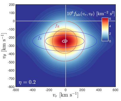
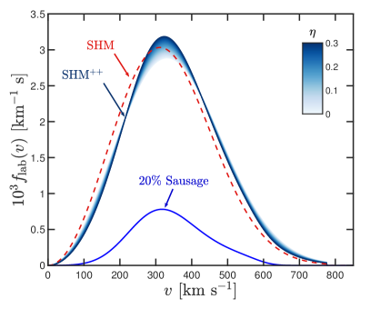
Figure 1: Left: Earth frame velocity distribution for the SHM⁺⁺ in the radial and horizontal directions. We assume a Sausage fraction of $\eta=0.2$. The shapes of the round component, $f_{R}(\mathbf{v})$, and Sausage component, $f_{S}(\mathbf{v})$, in velocity space are traced with red and blue contours respectively. The radial anisotropy of the Sausage component can be clearly seen. The white point marks the inverse of the velocity of the Sun (LSR + peculiar motion) and the white circle indicates the path of the full Earth velocity over one year. Right: Earth frame speed distributions for the SHM (red dashed) and the SHM⁺⁺ (blue). The shade of blue indicates the fraction of the halo comprised of Sausage. The lower blue line isolates only 0.2$f_{\rm S}(v)$. The effect of the Sausage component is to make the speed distribution colder.

In this section, we introduce the SHM⁺⁺ by carrying out two modifications to the SHM. First, and trivially, the local circular speed $v_{0}$, escape velocity $v_{\mathrm{esc}}$ and local DM density $\rho_{0}$ are updated in the light of more recent data. Second, and more fundamentally, we introduce a Sausage component to describe the radially anisotropic DM particles brought in by the Sausage galaxy.

III.1 Velocity Distributions

The velocity distribution of the bimodal dark halo in the frame of the Galaxy is described by

$$f(\mathbf{v})=(1-\eta)f_{\rm R}(\mathbf{v})+\eta f_{\rm S}(\mathbf{v})\,,$$ (3)

where $f_{\rm R}$ is the velocity distribution of the smooth, nearly round dark halo that dominates the gravitational potential in the innermost 20 kpc, whilst $f_{\rm S}$ is the velocity distribution of the Gaia Sausage. The parameter $\eta$ is a constant that describes the fraction of DM in the Sausage at the solar neighbourhood.

The nearly round dark halo component has a velocity distribution in the Galactic frame that is the familiar Gaussian distribution in Eq. (II) with $v_{0}=\sqrt{2}\sigma_{v}=233\pm 3$ kms^-1 as the speed of the LSR. This relation holds true provided the rotation curve is flat. The escape velocity used to cut off the velocity distribution is $v_{\mathrm{esc}}=528^{+24}_{-25}$ km s^-1 (Deason et al., 2019).

We now turn our attention to a velocity distribution for the highly radially anisotropic Gaia Sausage. The velocity dispersion tensor is aligned in spherical polar coordinates with $\sigma^{2}={\rm diag}(\sigma^{2}_{r},\sigma^{2}_{\theta},\sigma^{2}_{\phi})$. As the gravitational potential is close to spherical Evans et al. (2016); Wegg et al. (2018), then $\sigma_{\theta}=\sigma_{\phi}$. The anisotropy is parameterized by,

$$\beta=1-\frac{\sigma^{2}_{\theta}+\sigma_{\phi}^{2}}{2\sigma^{2}_{r}}\,,$$ (4)

which vanishes for an isotropic dispersion tensor. We recall that $\beta=1$ implies that all the orbits are completely radial and $\beta=-\infty$ that all the orbits are circular. The stellar debris associated with the Gaia Sausage has $\beta=0.9$ Belokurov et al. (2018); Myeong et al. (2018a). The Globular Clusters once associated with the Sausage Galaxy are in fact even more radially anisotropic with $\beta=0.95$ Myeong et al. (2018b). The anisotropy of the Sausage DM is unknown, though it too must be highly radial. We assume it is the same as the stellar debris $\beta=0.9$ in our standard model and assign an error of $\pm 0.05$.

The density distribution of the Sausage falls like $\sim r^{-3}$ (Iorio et al., 2018). The exact solution of the collisionless Boltzmann equation for an anisotropic tracer population with density falling like $r^{-3}$ in a galaxy with an asymptotically flat rotation curve is (Evans et al., 1997).

$$f_{\rm S}(\mathbf{v})=\frac{1}{(2\pi)^{3/2}\sigma_{r}\sigma_{\theta}^{2}N_{\mathrm{S,esc}}}\,\exp\left(-\frac{v_{r}^{2}}{2\sigma_{r}^{2}}-\frac{v_{\theta}^{2}}{2\sigma_{\theta}^{2}}-\frac{v_{\phi}^{2}}{2\sigma_{\phi}^{2}}\right)$$

$$\times\Theta(v_{\mathrm{esc}}-|\mathbf{v}|)\,,$$ (5)

The velocity dispersions are related to the amplitude of the rotation curve via (Evans et al., 1997)

$$\sigma_{r}^{2}=\frac{3v_{0}^{2}}{2(3-2\beta)},\qquad\sigma_{\theta}^{2}=\sigma_{\phi}^{2}=\frac{3v_{0}^{2}(1-\beta)}{2(3-2\beta)}\,,$$ (6)

where $v_{0}=233$ kms^-1 is the LSR.

The normalisation constant is

$$N_{\mathrm{S,esc}}=\mathrm{erf}\left(\frac{v_{\mathrm{esc}}}{\sqrt{2}\sigma_{r}}\right)-\left(\frac{1-\beta}{\beta}\right)^{1/2}\exp\left(-\frac{v_{\mathrm{esc}}^{2}}{2\sigma_{\theta}^{2}}\right)$$

$$\times\mathrm{erfi}\left(\frac{v_{\mathrm{esc}}}{\sqrt{2}\sigma_{r}}\frac{\beta^{1/2}}{(1-\beta)^{1/2}}\right),$$ (7)

where $\mathrm{erfi}$ is the imaginary error function. This is the anisotropic analogue of Eq. (2).

This completes our description of the velocity distribution of the SHM⁺⁺. It is an entirely analytic model of a roundish dark halo, together with a highly radially anisotropic Sausage component. It depends on the familiar Galactic constants already present in the SHM, namely the local circular speed $v_{0}$, the local escape speed $v_{\mathrm{esc}}$ and the local DM density $\rho_{0}$. There are two additional parameters in the SHM⁺⁺: the velocity anisotropy $\beta\approx 0.9\pm 0.05$ of the Gaia Sausage and the fraction of DM locally in the Sausage $\eta$, which we estimate in the next section.

On Earth, the incoming distribution of DM particles is found by boosting the DM velocities in the galactic frame by the Earth’s velocity with respect to the Galactic frame:  $\mathbf{v}_{\mathrm{E}}(t)=(0,v_{0},0)+(U,V,W)+\mathbf{u}_{\mathrm{E}}(t)$. Explicitly, this means that the Earth frame velocity distribution is $f_{\rm{lab}}(\mathbf{v})=f(\mathbf{v}+\mathbf{v}_{\mathrm{E}}(t))$. The Earth’s velocity is time dependent owing to the time dependence of $\mathbf{u}_{\mathrm{E}}(t)$, the Earth’s velocity around the Sun. Expressions for $\mathbf{u}_{\mathrm{E}}(t)$ are given in Refs. Lee et al. (2013); McCabe (2014); Mayet et al. (2016).

We plot the Earth frame distribution of velocities and speeds in Fig. 1. The velocity distribution (left panel) is displayed as the two-dimensional distribution $f_{\rm{lab}}(v_{r},v_{\theta})$, where we have marginalised over $v_{\phi}$. The blue contours associated with the Sausage component clearly show the radial bias in velocity space compared to the circular red contours associated with the round component of the halo. In the right panel, we show the speed distribution, $f_{\rm{lab}}(v)=v^{2}\int d\Omega f_{\rm{lab}}(\mathbf{v})$, for the SHM, SHM⁺⁺ and the isolated Sausage component. For the SHM distribution (red dashed line), we have used the parameters in the upper half of Table 1. For the SHM⁺⁺ distribution (blue shaded), we have used the parameters in the lower half of Table 1 with the exception of $\eta$, which we have allowed to vary in the range $\eta=0$ (corresponding to only a round halo component) to $\eta=0.3$. The solid blue line shows the contribution from only the Sausage component with $\eta=0.2$.

Comparing the SHM and SHM⁺⁺ distributions, we see that the SHM⁺⁺ distribution is everywhere shifted to higher speeds. This is primarily because of the larger value of $v_{0}$. Comparing the SHM⁺⁺ distribution with $\eta=0$ (the lightest edge in the shaded region) to the distribution with $\eta\neq 0$, we see that the impact of the Sausage component is to increase the peak-height of the speed distribution while decreasing the overall dispersion of the distribution, i.e. the Sausage component makes the total speed distribution colder compared to a halo with only the round, isotropic component. The difference in the dispersion arises from the different expressions for the velocity dispersions in the Sausage distribution ($f_{\rm S}$) compared to the round halo ($f_{\rm R}$).

III.2 Constraining $\eta$

The fraction $\eta$ of DM locally in the Gaia Sausage is not known, but an upper limit can be estimated. The stellar density distribution of the Sausage is triaxial with axis ratios $a=1$, $b=1.27\pm 0.03$, $c=0.57\pm 0.02$ near the Sun, and falls off like $\sim r^{-3}$ (Iorio et al., 2018). As a simple model, we assume that the Sausage DM density is stratified on similar concentric ellipsoids with ellipsoidal radius $m$

$$m^{2}={x^{\prime 2}\over a^{2}}+{y^{\prime 2}\over b^{2}}+{z^{2}\over c^{2}}.$$ (8)

Here, ($x^{\prime},y^{\prime}$) are the Cartesians in the Galactic plane, rotated so that the long axis $x^{\prime}$ is about $70^{\circ}$ with respect to the $x$-axis which conventionally connects the Sun and the Galactic Centre (Iorio et al., 2018).

The DM contribution of the triaxial Sausage cannot become too high, as it would then cause detectable perturbations (in the rotation curve or the kinematics of stars, for example) and would spoil the sphericity of the potential (Evans et al., 2016; Wegg et al., 2018). For large spirals like the Milky Way, the scatter in the Tully-Fisher relationship severely limits the ellipticity of the disk (Franx and de Zeeuw, 1992). In fact, the ellipticity of the equipotentials in the Galactic plane of the Milky Way must be less than 5 % on stellar kinematical grounds (Kuijken and Tremaine, 1994), almost all of which can be attributed to the Galactic bar Mühlbauer and Dehnen (2003). Any contribution to the ellipticity of the equipotentials in the Galactic plane from the Sausage must be less than $\sim 1\%$.

To estimate the dynamical effects of the Sausage, we need to compute the gravitational forces generated by an elongated, triaxial figure. For now we assume that the DM density falls in the same manner as the stars so the Sausage density within $m<30$ kpc is modelled by

$$\rho_{\rm S}(m^{2})={\rho_{a}r_{a}^{3}\over(r_{a}^{2}+m^{2})^{3/2}}.$$ (9)

The virtue of this model is that the gravitational potential of the Sausage at any point is then known (Chandrasekhar, 1987)

$$\phi=-4\pi G\rho_{a}abcR_{\rm F}(\lambda,\mu,\nu)\;,$$ (10)

where $R_{\rm F}$ is the Carlson elliptic integral and ($\lambda,\mu,\nu$) are ellipsoidal coordinates. The total mass within ellipsoidal radius $m$ is

$$M(m)=4\pi abc\,r_{a}^{3}\,\rho_{a}\Bigl{[}\log([m+\sqrt{r_{a}^{2}+m^{2}}]/r_{a})$$ (11)

$$-{m\over\sqrt{r_{a}^{2}+m^{2}}}\Bigr{]}\;.$$

Although the total mass diverges logarithmically, this is not a problem as by Newton’s theorem, ellipsoidal shells of constant density have no dynamical effects inside the shell.

We now constrain the mass of the Sausage within 30 kpc, or $M(30)$. The Sausage contributes a monopole component which provides a small part of the local circular velocity speed of $v_{0}=233$ kms^-1. The remainder is provided by the rest of the Galaxy. This is modelled as a logarithmic potential with an amplitude chosen so that, when its circular speed is added in quadrature to that of the Sausage, the local circular speed of 233 kms^-1 is correctly reproduced. Requiring the ellipticity of the combined equipotentials in the plane to be less than 1% imposes an upper limit on the mass of the Sausage $M(30)$ of $\lesssim 3\times 10^{10}M_{\odot}$. Using the density law Eq. (9), we find the fraction of DM in the Solar neighbourhood due to the Sausage is $\eta\lesssim 20\%$.

There are arguments suggesting that this limit may be an overestimate – for example, the DM is always more extended than the luminous matter in dwarf galaxies. Tidal stripping of an infalling satellite therefore distributes DM over a much large volume than the luminous matter, so our use of $\sim 30$ kpc inspired by the stellar debris may be unwarranted. The density law of the DM may also be different from the $r^{-3}$ fall-off of the stars. However, there are also arguments suggesting that this may be an underestimate – for example, the velocity distribution of the stellar debris Lancaster et al. (2018b) suggests that the stellar density is depleted in the very innermost parts. If the same is true of the DM, then our calculation may not ascribe enough DM to the solar neighbourhood. Given all the uncertainties, it is therefore prudent to allow $\eta$ to vary within the range $10\%$ to $30\%$ with a preferred value of $20\%$. This is consistent with recent numerical work from the Auriga (Fattahi et al., 2018) and the FIRE simulations (Necib et al., 2018).

IV Comparisons with Alternatives

Our derivation of the SHM⁺⁺ is based upon equilibrium distribution functions, together with a collection of robust astronomical measurements. The main advantage of our model is that it is both simple and accounts for known properties of the Milky Way halo.

However, it is not the only method that has been used to infer the local DM velocity distribution. Recently, there have been attempts to deduce the velocity distribution empirically using observations of low metallicity halo stars. We can also resort to numerical simulations to gain more understanding of the behaviour of DM inside galactic halos. We discuss possible overlaps and disagreements with these various methods here.

IV.1 Low and Intermediate metallicity halo stars

An alternative suggestion as to an appropriate velocity distribution is motivated by the claim that the metal-poor halo stars are effective tracers of the local DM distribution (Herzog-Arbeitman et al., 2018a). This claim has inspired DM velocity distributions based on the empirical properties of the velocities of the metal-poor stars in RAVE or SDSS-Gaia (Herzog-Arbeitman et al., 2018b; Necib et al., 2018). However, if the velocity distributions of any two populations are the same, and they reside in the same gravitational potential, then their orbital properties are also the same. In gravitational physics, the density of stars or DM is built up from their orbits. So, the assumption is equivalent to assuming that the density of the stars and DM are the same. This remains true even if the potential is not steady.

Hence, the hypothesis of Refs. Herzog-Arbeitman et al. (2018a, b); Necib et al. (2018) is equivalent to assuming that the density distributions of the metal-poor halo stars and the DM are the same (up to an overall normalization). This is known to be incorrect, as the density of the metal-poor stars (or any stellar component) falls too quickly with Galactocentric radius to provide the flatness of the Milky Way’s rotation curve. This causes the local velocity distribution of low metallicity halo stars to be much colder than the DM. Consequently, if the DM velocity distribution is assumed to follow the metal-poor stars, then the dark matter speeds will be under-estimated (as their orbits no longer provide the density at large radii to make the rotation curve flat). This leads to the conclusion that the DM is colder than is really the case. Our argument is corroborated by results from the Auriga simulations Grand et al. (2017), where the speed profiles of low metallicity stars in the simulated halos are indeed colder than the DM speed distributions Bozorgnia et al. (2018).

Of course, the DM may have multiple sub-populations, some of which track the stellar density distributions and some of which do not. In fact, this is seen in some of the insightful examples provided in the FIRE simulations Necib et al. (2018). Then of course the density of stars and DM can be different. However, if only a minority of the DM tracks the stellar density, then the analogy is of only partial help in providing velocity distributions for direct detection experiments.

In the picture of Ref. Necib et al. (2018), the correspondence between the metal-poor stars and dark matter pertains only to the oldest luminous mergers that build the smooth, nearly round dark halo (our $f_{\rm R}$). The Sausage stars are of intermediate metallicity, and here the assumption is that they trace the DM brought in by the merger event. The humped structure in $f(v_{r})$ with two lobes at $v_{r}=\pm 148$ km s^-1 is associated with the apocentric pile-up at $\sim 30$ kpc that marks the density break in the stellar halo Lancaster et al. (2018a). They will not exist for the Sausage DM velocity distribution, as the DM density profile does not break at $\sim 30$ kpc. The DM from the Sausage Galaxy was originally more extended than the stars in the progenitor and so was stripped earlier and is likely sprawled over much larger distances. In simulations of sinking and radializing satellites, the length scale of the DM tidally torn from the satellite exceeds that of the stars by typically a factor of a few  (e.g., Amorisco, 2017; Fattahi et al., 2018). The density of the tidally stripped stars and DM from the Sausage Galaxy will also therefore be quite different.

IV.2 Simulations

Our data-driven work is complementary to the approach adopted in Refs. Bozorgnia et al. (2016); Kelso et al. (2016); Sloane et al. (2016); Lentz et al. (2017). Here, simulated halos built up from successive merger events are examined to extract better motivated velocity distributions than the SHM ansatz. In part, this is also an attempt to understand the connections present between the dark and baryonic matter distributions of galactic halos. A detailed summary of the findings of a collection of simulations and their implications for direct detection can be found in Ref. Bozorgnia and Bertone (2017).

Several of these studies confirm that the Maxwellian speed distribution derived from the SHM is satisfactory for the purposes of direct detection signal modelling. Refs. Bozorgnia et al. (2016); Bozorgnia and Bertone (2017) raise the caveat that in some simulations, the circular speed $v_{0}$ and peak speed of the distributions are different, though this was not found in Kelso et al. (2016).

A key difference in our approach is that we have made a bespoke velocity distribution to account for a known merger event in the Milky Way’s recent history. In the future, the complementarity between our approach and numerical simulations will grow, as we can use simulations to understand more about the impact of this merger on the local DM distribution. Ultimately this will put both data-driven and simulation-driven predictions of experimental DM signals on more robust grounds.

V Experimental consequences

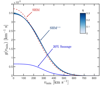
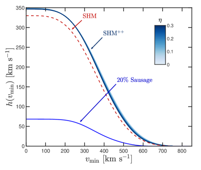
Figure 2: The two halo integrals outlined in the text that enter the rate calculation for nuclear recoil signals: the mean inverse speed $g(v_{\rm min})$ (left) and mean speed $h(v_{\rm min})$ (right). We show their shapes for both the SHM and SHM⁺⁺ as a red line and blue region respectively. We take the value of these functions averaged over time. Direct detection event rates are linearly proportional to one or both of these integrals. The blue shading indicates the value of the Sausage density fraction, $\eta$. The Sausage component with $\eta=0.2$ is isolated as a blue line.

The purpose of a standard benchmark halo model is to facilitate the self-consistent mapping of exclusion limits on the properties of a DM particle candidate. Since all detection signals require this input, all are influenced by changing the model of the local distribution of DM. In this section, we demonstrate in simple terms the differences brought about by the bimodal distribution of the SHM⁺⁺. As examples, we consider the two most popular candidates for DM: weakly interacting massive particles (WIMPs) and axions. For WIMPs, we show the effect of the Sausage on nuclear recoil event rates (Sec. V.1) and cross section limits (Sec. V.2), as well as differences in their directional signals (Sec. V.3). For axions (Sec. V.4), the discussion is more straightforward and can be summarised with a simple formula encapsulating the consequences of different signal model assumptions.

V.1 Nuclear recoil signals

There are many experiments actively searching for the nuclear recoil energy imparted by the collision of a DM particle with a nucleus. For these two-to-two scattering processes (which could be elastic or inelastic collisions Tucker-Smith and Weiner (2001); Baudis et al. (2013); McCabe (2016)), the general formula for the differential scattering rate $R$ of nuclear recoil events as a function of the nuclear recoil energy $E_{r}$ is

$$\frac{\textrm{d}R(t)}{\textrm{d}E_{r}}=N_{T}\frac{\rho_{0}}{m_{\chi}}\int_{v>v_{\rm min}}\!\!\!\!v\,f\big{(}\mathbf{v}+\mathbf{v}_{\mathrm{E}}(t)\big{)}\,\frac{d\sigma_{T}(v,E_{r})}{dE_{r}}\,\textrm{d}^{3}v\,.$$ (12)

Here, $N_{T}$ is the number of target nuclei in the experiment, $m_{\chi}$ is the DM mass, $v=|\mathbf{v}|$ is the DM speed in the reference frame of the experiment, $v_{\rm{min}}$ is the minimum DM speed that can induce a recoil of energy $E_{r}$, $\sigma_{T}$ is the DM–nucleus scattering cross section, which in general depends on $v$ and $E_{r}$, and finally $f(\mathbf{v+v_{\mathrm{E}}}(t))$ is the DM velocity distribution boosted to the Earth’s frame.

For the canonical leading order spin-independent (SI) and spin-dependent (SD) DM–nucleus interactions Marrodan Undagoitia and Rauch (2016), the differential cross section is inversely proportional to the square of the DM speed, $d\sigma_{T}/dE_{r}\propto v^{-2}$. For these interactions, all of the dependence on the DM velocity distribution is encapsulated in the function

$$g(v_{\rm min},t)=\int_{v>v_{\rm min}}\frac{f(\textbf{v}+\mathbf{v}_{\mathrm{E}}(t))}{v}\,\textrm{d}^{3}v\,.$$ (13)

More general two-to-two DM–nucleus interactions can be parameterized in the non-relativistic effective field theory framework for direct detection Fitzpatrick et al. (2013, 2012); Anand et al. (2014), which allows for any Galilean invariant and Hermitian interaction that respects energy and momentum conservation. Within the effective field theory framework, direct detection signals depend on a linear combination of $g(v_{\rm min},t)$ and $h(v_{\rm min},t)$, which is defined as

$$h(v_{\rm min},t)=\int_{v>v_{\rm min}}vf(\textbf{v}+\mathbf{v}_{\mathrm{E}}(t))\,\textrm{d}^{3}v\,.$$ (14)

We show $g(v_{\rm min},t)$ and $h(v_{\rm min},t)$ in Fig. 2. For the SHM, there exist analytic expressions for these integrals (see e.g. Savage et al. (2006); McCabe (2010); Fitzpatrick and Zurek (2010)). For the SHM⁺⁺, there are no known analytic expressions, though they are easily evaluated numerically. The blue shaded region corresponds to the SHM⁺⁺ with the Sausage fraction in the range $0.1\leq\eta\leq 0.3$. The dashed red line shows the result for the SHM with the parameters in Tab 1. For the mean inverse speed, $g(v_{\rm min})$, the SHM⁺⁺ produces a slightly different shape leading to a suppression of around 10% for $v_{\rm min}<200\textrm{ km s}^{-1}$ and a much smaller increase over speeds $v_{\rm min}>200\textrm{ km s}^{-1}$. The inclusion of the Sausage component leads to a small change in the shape of the mean speed integral, $h(v_{\rm min})$, but there is a persistent increase of around 6% in the SHM⁺⁺ relative to the SHM. This increase reflects the 6% increase in $v_{0}$ in the SHM⁺⁺.

At first sight, it may seen surprising that the differences between the SHM and SHM⁺⁺ models are not greater. The resolution lies in the fact that we have made multiple counter-balancing changes to the SHM. The relative coldness of the new Sausage DM is counteracted by the increased hotness of the halo DM due to the increase in $v_{0}$.

With $g(v_{\rm min},t)$ in hand, we compare the rate and exclusion limits in the SHM and SHM⁺⁺ for the most commonly studied interaction: the spin-independent DM-nucleus interaction, in which the differential cross section takes the form:

$$\frac{d\sigma_{T}(v,E_{r})}{dE_{r}}=\frac{m_{N}A^{2}\sigma_{p}^{\rm{SI}}}{2\mu_{p}^{2}\,v^{2}}F^{2}(E_{r})\;,$$ (15)

where $m_{N}$ is the nucleus mass, $A$ is the atomic number, $\mu_{p}$ is the DM-proton reduced mass, $F(E_{r})$ is the nuclear form factor and $\sigma_{p}^{\rm{SI}}$ is the DM-proton scattering cross section.

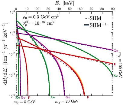
Figure 3: Spin-independent differential event rate as a function of energy for the SHM (dashed) and SHM⁺⁺ (shaded, indicating a range of $\eta$, as in Figs. 1 and 2). The rates for three target nuclei are shown: xenon (green), germanium (purple) and fluorine (red). We also show results for three different values of the DM mass (5, 20 and 100 GeV for rates extending from the lowest to the highest energies shown). We have fixed $\rho_{0}=0.3$ GeV ​cm³ for the SHM and SHM⁺⁺ spectra to show only the changes due to the velocity distributions.

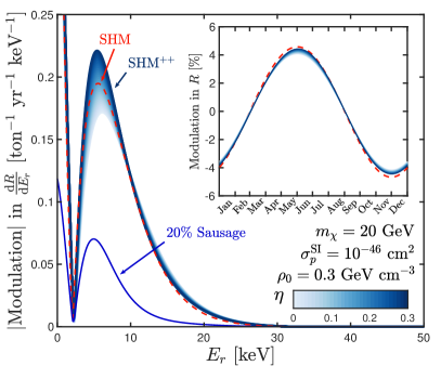
Figure 4: Annual modulation of the SI differential event rate (main) and total rate (inset) for DM with a mass of 20 GeV scattering off a xenon nucleus. The blue shaded region corresponds to the SHM⁺⁺ with varying $\eta$ whereas the dashed red line is the SHM. As in Fig. 3, we have fixed $\rho_{0}=0.3\textrm{ GeV cm}^{-3}$ for both the SHM and SHM⁺⁺ to again isolate the changes brought about by the velocity distributions.

We show the differential event rate as a function of recoil energy in Fig. 3 for a three different target nuclei: ¹³¹Xe (green), ⁷⁴Ge (purple) and ¹⁹F (red). In this figure, we have temporarily fixed the local DM density at $\rho_{0}=0.3\textrm{ GeV cm}^{-3}$ for both models. This is so that we can highlight only the difference arising from the change in velocity distribution, rather than the simple rescaling by the new value of $\rho_{0}$. Three different values of the DM mass are shown and as in previous figures, the shading indicates the effect of the Sausage component. Consistent with the rather minor alterations seen in $g(v_{\rm min})$, there are only modest changes in the recoil energy spectra, mainly in the high-energy tails of the spectra. The spectra with only a round halo, corresponding to $\eta=0$, and with the updated astrophysical parameters in the lower half of Table 1 are shown by the lightest colour in the shaded region. We see that increasing $\eta$ slightly reduces the maximum energy for all cases.

The differential modulation event rate, defined as $dR/dE_{r}\large|_{\rm{max}}-dR/dE_{r}\large|_{\rm{min}}$, is shown in the main panel of Fig. 4. We assume here a DM mass of 20 GeV scattering with xenon. As in previous figures, the red-dashed line shows the rate for the SHM, the blue-shaded regions shows the rate for the SHM⁺⁺ for different values of $\eta$ and the blue line shows the contribution from the Sausage component with $\eta=0.2$. We have again fixed $\rho$ to be the same for the SHM and SHM⁺⁺ spectra. As in the previous figures, the changes between the two models are relatively small. Increasing the contribution of the Sausage component has the effect of increasing the peak modulation amplitude while slightly decreasing the higher energy modulation spectrum.

The inset in Fig. 4 shows the modulation in the total scattering rate, $R$, over the course of one year. Importantly, we note that the Sausage component of the halo is modulating essentially in phase with the isotropic part. Recall that the modulation of the event rate is controlled by relative velocity between the motion of the Earth and the direction in velocity space that the distribution is boosted. Since both the halo and the Sausage are centred at the origin in velocity space, they are both boosted to the same new centre in the Earth frame (see Fig. 1). In fact it is only features that are off-centred in velocity space, such as streams, that can give rise to significant phase changes in the annual modulation signal Savage et al. (2006); O’Hare et al. (2018).

V.2 Impact on cross section limits

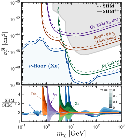
Figure 5: Top: Using a set of toy experimental setups, we demonstrate the impact of the SHM⁺⁺ on the sensitivity limits for three classes of detectors: a germanium experiment (purple), a directional He:SF₆ experiment (orange) and a xenon experiment (green). The lower blue shaded region shows the neutrino floor for a xenon target while the grey shaded region shows the already excluded parameter space (assuming the SHM). The dashed lines indicate the sensitivity assuming the SHM while the solid lines assume the SHM⁺⁺. For the SHM⁺⁺ limits in the top panel, we have used the parameters from the lower half of Table 1. Bottom: The ratio between the SHM and the SHM⁺⁺ cross sections. The shading indicates the ratio for different values of $\eta$ ($\eta=0.2$ corresponds to the ratio for the top panel). The black dotted line indicates the difference that arises solely from the different values of $\rho_{0}$ in the SHM and SHM⁺⁺; deviations from this line arise from the different velocity distributions.

The results of direct detection experiments are usually summarised in terms of exclusion limits on the SI DM-proton scattering cross section as a function of DM mass. In Fig. 5, we illustrate the effects of moving from the SHM to the SHM⁺⁺ for three hypothetical experiments using a xenon (green), germanium (purple) and a He:SF₆ (red) target material. In the upper panel, the dashed lines show the limits for the SHM with parameters in the upper half of Table 1, while the solid lines show the limits for the SHM⁺⁺ with our new recommended values for the astrophysical parameters given in the lower half of Table 1. The limits are calculated as median discovery limits, where we use the profile likelihood ratio test under the Asimov approximation to calculate the cross sections discoverable at 3$\sigma$ (see Ref. Cowan et al. (2011) for more details). WIMP 90% CL exclusion limits will follow the same behaviour as the discovery limits shown in Fig. 5.

The green limits correspond to a toy version of a liquid xenon experiment like DARWIN Aalbers et al. (2016) with a $\sim$200 ton-year exposure. As a proxy, we have used the background rate and efficiency curve reported for LZ Akerib et al. (2018). The low threshold germanium result (purple limits) is a toy version of the SuperCDMS Agnese et al. (2018) or EDELWEISS Arnaud et al. (2018) experiments, where we assume a simple error function parameterisation for the efficiency curve, which falls sharply towards a threshold at 0.2 keV. The He:SF₆ target (red limits) is a toy version of the 1000m³ CYGNUS directional detector using a helium and SF₆ gas mixture (discussed in more detail in Sec. V.3). We have also included realistic estimates of the detector resolutions in our results.

The upper gray shaded regions in Fig. 5 show the existing exclusion limits on the SI WIMP-proton cross section (calculated assuming the SHM with the parameters in the upper half of Table 1). This is an interpolation of the limits of (from low to high masses) CRESST Angloher et al. (2016), DarkSide-50 Agnes et al. (2018), LUX Akerib et al. (2017b), PandaX Tan et al. (2016) and XENON1T Aprile et al. (2018). The lower blue region shows the ‘neutrino floor’ region for a xenon target. The neutrino floor delimits cross sections where the neutrino background saturates the DM signal, so is therefore dependent upon the shape of the signal model that is assumed O’Hare (2016). We calculate the floor in the same manner as described in Refs. Billard (2014); Ruppin et al. (2014); O’Hare (2016)

Fig. 5 shows a noticeable shift between the SHM and SHM⁺⁺ limits. This is mostly due to the different values of $\rho_{0}$, which can be most clearly seen from examining the ratio between the limits shown in the lower panel. The black dotted line in the lower panel indicates the ratio 0.55/0.3, the ratio of the different $\rho_{0}$ values. It is only as the limits approach the lowest DM mass to which each experiment is sensitive that the ratio of cross sections deviate significantly from the black dotted line. The small impact on the shape of the exclusion limits can be understood as follows. Contrasting the SHM and SHM⁺⁺ signals, there are two competing effects which act to push the limits in opposite directions. Increasing $v_{0}$ strengthens the cross section limits because it increases the number of recoil events above the finite energy threshold. However, the Sausage reverses this effect since, as we saw in Fig. 3, the Sausage component decreases the maximum recoil energy so there are fewer events above the finite energy threshold.

The neutrino floor has a more complicated relationship with the velocity distribution and the WIMP mass. The cross section of the floor depends upon how much the neutrino background overlaps with a given DM signal. The neutrino source that overlaps most with a DM signal depends on $m_{\chi}$. This leads to the non-trivial dependence of the neutrino floor on the Sausage fraction $\eta$ shown in the lower panel.

Altogether, our refinement of the SHM ultimately leads to only slight changes to the cross section limits which, for the most part, are simple to understand. This can be considered a positive aspect of our new model, since while it includes refinements accounting for the most recent data, it simultaneously allows existing limits on DM particle cross sections to be used with confidence. The most notable difference in the limits arises from the larger value of $\rho_{0}$, which can be implemented trivially as an overall scaling. In the event of the positive detection of a DM signal, which would lead to closed contours in the mass–cross section plane, the use of the wrong model could lead to an incorrect bias in the measurement of both the DM mass and cross section. Our refinements to the halo model will be even more important to consider in the context of a discovery so that any bias is minimised.

V.3 Directional signals

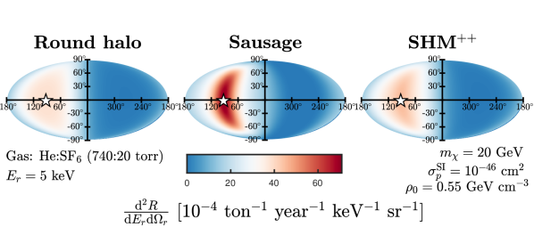
Figure 6: Mollweide projection in galactic coordinates of the value of the double differential angular recoil rate as a function of the inverse of the recoil direction $-\hat{\mathbf{q}}$ at a fixed recoil energy of 5 keV. We assume a 20 GeV DM mass and sum the rates from both He and SF₆. The panels from left to right show the distributions for distribution of the round halo component, the Sausage, and the combined SHM⁺⁺ respectively. The Sausage component gives rise to a distinctive pattern compared to the round halo. We indicate the direction of $\mathbf{v}_{\mathrm{E}}$ with a white star.

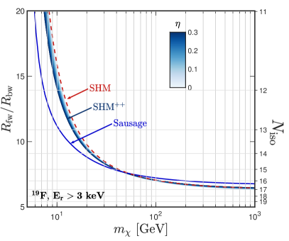
Figure 7: Anisotropy of the WIMP directional signal as a function of WIMP mass. We quantify this anisotropy as the ratio of the total event rate in the forward hemisphere $R_{\rm fw}$ (pointing towards $-\mathbf{v}_{\mathrm{E}}$) relative to the rate in the backward hemisphere $R_{\rm bw}$ (pointing towards $\mathbf{v}_{\mathrm{E}}$). The blue region corresponds to the SHM⁺⁺ with $\eta=0$ to 30%. The red dashed line shows the anisotropy for the SHM. The anisotropy of the Sausage alone is shown as the blue line. Here we integrate above a recoil energy threshold of 3 keV. On the right hand axis we indicate the approximate number of events to detect the anisotropy at the same position on the left hand axis.

The main difference between the kinematic structures of the round halo and the Sausage are at the level of the full three-dimensional velocity distribution. Much of this structure is integrated away when computing the speed distribution and the integrals that depend on it. To appreciate the full impact of the Sausage component, we should consider experiments which are not only sensitive to the speed of incoming DM particles but also their direction. Such directional detectors are well motivated on theoretical grounds (see Ref. Mayet et al. (2016) for a review) because the signal from an isotropic DM halo gives a distribution of recoil angles that aligns with Galactic rotation Spergel (1988), thus clearly distinguishing it from any background Grothaus et al. (2014); O’Hare et al. (2015, 2017). Directional detectors preserve much more kinematic information about the full velocity distribution Morgan et al. (2005); Billard et al. (2010); Lee and Peter (2012); O’Hare and Green (2014); Mayet et al. (2016); Kavanagh and O’Hare (2016).

For directionally sensitive detectors, the double differential event rate as a function of recoil energy, recoil direction and time is proportional to an analogous halo integral, called the Radon transform Gondolo (2002); Deans (1983),

$$\hat{f}(v_{\rm min},\hat{\mathbf{q}},t)=\int\delta\left(\textbf{v}\cdot\hat{\mathbf{q}}-v_{\rm min}\right)f(\textbf{v}+\textbf{v}_{\mathrm{E}}(t))\,\textrm{d}^{3}\textbf{v}\,,$$ (16)

where $\hat{\mathbf{q}}$ is the direction of the recoiling nucleus. This enters into an analogous formula to Eq. (12) for the double differential recoil rate with energy and angle, $\textrm{d}^{2}R/\textrm{d}E_{r}\textrm{d}\Omega_{r}$.

Directional detectors are challenging to build, as Refs. Ahlen et al. (2010); Battat et al. (2016) discuss. Many ideas have been proposed to develop detector technologies with angular recoil sensitivity, including nuclear emulsions Nygren (2013); Li (2015) and columnar recombination Aleksandrov et al. (2016); Agafonova et al. (2017) for nuclear recoils, as well as several novel engineered materials for electron recoils Griffin et al. (2018); Hochberg et al. (2016, 2018). Experimentally the most developed technique for is to use gaseous time projection chambers (see Refs. Daw et al. (2012); Battat et al. (2015, 2016); Monroe (2012); Leyton (2016); Santos et al. (2012); Riffard et al. (2013); Nakamura et al. (2015)). A large-scale gaseous time projection chamber called CYGNUS has been proposed and a feasibility study is currently underway Battat et al. (2018). Two gases are under investigation for CYGNUS: SF₆ at 20 torr and ⁴He at 740 torr. Both have a total mass of 0.16 tons for a 1000 m³ experiment at room temperature. Based on these targets we show $\textrm{d}^{2}R/\textrm{d}E_{r}\textrm{d}\Omega_{r}$, for the round halo (left), Sausage (middle) and the SHM⁺⁺ (right) in Fig. 6. Fixing the recoil energy to $E_{r}=5$ keV, we display the full-sky map of recoil angles, which clearly show a distinctive pattern for the Sausage component when compared with the round halo. Furthermore this effect is preserved even when the Sausage is a sub-dominant contribution to the full model.

In Fig. 7, we show the ratio of $R_{\rm fw}$ to $R_{\rm bw}$. $R_{\rm fw}$ is the total rate for scattering with fluorine above $E_{r}=3$ keV in the hemisphere centred around $-\mathbf{v}_{\mathrm{E}}$, while $R_{\rm bw}$ is the total rate in the opposite hemisphere. This ratio therefore gives a measure of the anisotropy of the WIMP directional signal. Fig. 7 shows that the Sausage component decreases the anisotropy of the WIMP directional signal, albeit by a modest amount.

We can also express the same behaviour as a function of $N_{\rm iso}$, which is an approximate lower limit to the number of events required to detect the dipole anisotropy at 3$\sigma$. To detect the anisotropy, we require that the contrast in event numbers in the forward/backward hemisphere ($N_{\rm fw}-N_{\rm bw}$) is greater than the typical 3$\sigma$ random deviation expected under isotropy, 3$\sqrt{N_{\rm fw}+N_{\rm bw}}$. Expressed in terms of event rates gives the formula,

$$N_{\rm iso}\approx\left(3\,\frac{R_{\rm fw}+R_{\rm bw}}{R_{\rm fw}-R_{\rm bw}}\right)^{2}\,.$$ (17)

As higher energy recoils typically have smaller scattering angles, more of the anisotropy of the DM flux is preserved in the tail of $\textrm{d}R/\textrm{d}E_{r}$. Hence the anisotropy increases toward the lowest masses displayed in Fig. 7, where only the tail of the recoil energy distribution is above threshold.

The Sausage component (the blue line in Fig. 7) is considerably less anisotropic than the round halo. This is because the population of DM in the Sausage is hotter in the radial direction, meaning a greater number of recoils scatter away from $\mathbf{v}_{\mathrm{E}}$ above a given energy threshold. This effect is exaggerated at low masses when the only observable particles from the Sausage are those with the most strongly radial orbits. At high masses, when the observable part of the recoil energy spectrum samples a much larger portion of the velocity distribution, the SHM and SHM⁺⁺ nearly converge. When looking at the full Radon transform down to much lower $v_{\rm min}$, the Sausage signal is only slightly more anisotropic than the round halo. This is for two reasons. Firstly, the increased hotness in the radial direction of the triaxial Gaussian is compensated by an increased coldness in the tangential direction (aligning with $\mathbf{v}_{\rm E}$). Secondly, much of the anisotropy of the signal becomes washed out in the stochastic process of elastic scattering.

Nevertheless, the Sausage is a noticeably different class of feature in the angular distribution of recoils. This means that, in the event of a detection, a directional experiment would have a better chance of distinguishing between the Sausage-less model of the halo and the SHM⁺⁺ compared to an experiment with no directional information. We anticipate that the Sausage will also have an impact on higher order directional features Bozorgnia et al. (2012a, b), the time integrated signal O’Hare et al. (2017), and angular signatures of operators with transverse velocity dependence Kavanagh (2015); Catena (2015), but for brevity we leave these to future studies.

V.4 Axion haloscopes

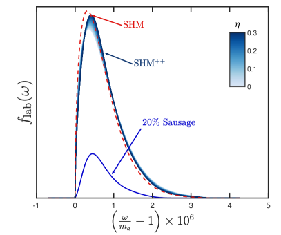
Figure 8: Spectral lineshape observable in an axion haloscope. We show only the shape of the signal distribution as a function of frequency $\omega$, scaled by the axion mass $m_{a}$. As in previous figures the red dashed line shows the SHM, whereas the blue region shows the new signal model from the SHM⁺⁺, shaded to indicate the range of values of $\eta$. We also isolate a 20% contribution from the Sausage, shown as a blue line.

The detection of axions is different from WIMPs and requires a different procedure to demonstrate the effect of the new halo model. To detect axions, the standard approach is to attempt to convert them into photons inside the magnetic field of some instrument. In the event of a detection, the electromagnetic response from axion-photon conversion can be measured in such a device as a function of frequency. The frequency of the electromagnetic signal is given by $\omega=m_{a}(1+v^{2}/2)$, so the spectral distribution of photons measured over many coherence times of the axion field oscillations will approach the astrophysical distribution of speeds on Earth, $f_{\rm{lab}}(v)$ (cf. Fig. 1). To identify the frequency of the axion mass, $m_{a}$, the experiment may either enforce some resonance or constructive interference condition for a signal oscillating at $\omega=m_{a}$ (as in e.g. ADMX Asztalos et al. (2010); Du et al. (2018), MADMAX Caldwell et al. (2017); Brun et al. (2017); Millar et al. (2017), HAYSTAC Brubaker et al. (2017b); Rapidis (2018); Brubaker et al. (2017a); Zhong et al. (2018); Brubaker (2017), CULTASK Chung (2016); Lee (2017); Chung (2017), Orpheus Rybka et al. (2015), ORGAN McAllister et al. (2017, 2018a), KLASH Alesini et al. (2017) and RADES Melcon et al. (2018)), or be sensitive to a wide bandwidth of frequencies simultaneously (e.g. ABRACADABRA Kahn et al. (2016); Foster et al. (2018); Henning et al. (2018), BEAST McAllister et al. (2018b) and DM-Radio Silva-Feaver et al. (2016)). The axion signal lineshape has a quality factor of around $10^{6}$ so even in the best resonant devices, the full axion signal will be measured at once. This means that in both resonant and broadband configurations, the sensitivity to axions is dependent upon how prominently the signal can show up over a noise floor. For a recent review of experiments searching for axions see Ref. Irastorza and Redondo (2018).

The axion spectral density is proportional to the speed distribution, up to a change of variables between frequency and speed (see e.g. Refs. O’Hare and Green (2017); Foster et al. (2018))

$$\frac{\textrm{d}P}{\textrm{d}\omega}=\pi\mathcal{H}(\omega)\,g^{2}_{a\gamma}\,\rho_{0}\,f_{\rm{lab}}(\omega)\,,$$ (18)

where $\mathcal{H}(\omega)$ encodes experimental dependent factors and $g_{a\gamma}$ is the axion-photon coupling on which the experiment will set a limit. The shape of the axion signal is dominated by the term

$$f_{\rm{lab}}(\omega)=\frac{\textrm{d}v}{\textrm{d}\omega}\,f_{\rm{lab}}(v)\,,$$ (19)

since the frequency dependence of $\mathcal{H}(\omega)$ in any realistic experiment will be effectively constant over the small range of frequencies covered by galactic speeds. We show $f_{\rm{lab}}(\omega)$ as a function of frequency in Fig. 8. This distribution is similar to $f_{\rm{lab}}(v)$, which was presented in Fig. 1, but is now a function of the observable quantity in an axion experiment.

The statistical methodology of a generic axion DM experiment consists of the spectral analysis of a series of electromagnetic time-stream samples. The stacking of the Fourier transforms of this time-stream data in most cases leads to Gaussian noise suppressed by the duration of the experiment, as well as (ideally) an enhanced axion signal on top. Hence a likelihood function for such data can be written in terms of a $\chi^{2}$ sum over frequency bins which ultimately can be approximated in terms of the integral over the power spectrum squared. Since the power is proportional to $g^{2}_{a\gamma}$, the minimum discoverable value scales with the shape of the signal as Foster et al. (2018),

$$g_{a\gamma}\propto\sqrt{\frac{1}{\rho_{0}}}\left(\int_{m_{a}}^{\infty}\mathrm{d}\omega\,f_{\rm{lab}}(\omega)^{2}\right)^{-1/4}\,.$$ (20)

This formula encodes the fact that signals that are sharper in frequency are more prominent over white noise and hence easier to detect. However, the dependence on the width of $f_{\rm{lab}}(\omega)$ and therefore the width of $f_{\rm{lab}}(v)$ only enters weakly, as an integral raised to the $-1/4$ power, so although the SHM⁺⁺ distribution is colder, the overall effect is small. Additionally, the Sausage component is not especially localized at a given frequency so again, its impact is small. For demonstration, a hypothetical experiment which used an $\eta=1$ signal model would set limits on $g_{a\gamma}$ only around 6% stronger that the same experiment using $\eta=0$.

For the parameters in Table 1 – modulo the value $\rho_{0}=0.45\textrm{ GeV cm}^{-3}$ instead of $\rho_{0}=0.3\textrm{ GeV cm}^{-3}$ in the SHM to reflect the preference of haloscope collaborations – constraints on $g_{a\gamma}$ assuming the SHM⁺⁺ relative to the the SHM are around 8% stronger. As in the case of WIMPs , there are several competing effects. The increase in $v_{0}$ acts to broaden the signal line-width making constraints weaker. However the inclusion of the Sausage component, which is a slightly sharper signal, balances against this. Based on the difference in shapes of $f_{\rm{lab}}(v)$ alone, constraints when using the SHM⁺⁺ would be about 2% weaker. The final balancing act comes from the new increased value of $\rho_{0}$. This ultimately has the greatest impact and pushes the SHM⁺⁺ constraint to be stronger than the SHM.

The sensitivity of axion haloscopes to astrophysics is essentially only controlled by the width of the speed distribution (rather than moments above some cutoff as is the case for WIMPs). Hence it is not surprising that the refinements that we have made have little impact on limits on the axion-photon coupling. As has been discussed in the past, the only changes that can bring significant changes to the axion signal are cold substructures like streams, which present highly localised peaks in frequency O’Hare and Green (2017); Foster et al. (2018); Knirck et al. (2018); O’Hare et al. (2018). One exception may be directional axion experiments possessing sensitivity to the full velocity distribution via prominent diurnal modulations Irastorza and Garcia (2012); Knirck et al. (2018). These will be altered significantly by the Sausage component, however such experiments remain hypothetical.

VI Conclusions

The data from the Gaia satellite Gaia Collaboration et al. (2018) has driven many changes in our picture of the Milky Way Galaxy. Firstly, more prosaically, it has enabled the uncertainties in many Galactic parameters to be substantially reduced. The halo shape (Sec. II.1), circular speed (Sec. II.2) and the escape speed (Sec. II.3) are now much more securely pinned down than before. Only the local DM density (Sec. II.4) remains obdurately uncertain, though analyses in the near future of Gaia Data Release 2 should improve constraints on its value.

Secondly and more spectacularly, it has provided unambiguous evidence of an ancient head-on collision with a massive ($10^{10}-10^{11}\,\textrm{M}_{\odot}$) satellite galaxy  Kruijssen et al. (2018); Myeong et al. (2018a); Belokurov et al. (2018); Mackereth et al. (2018), reinforcing earlier suggestions that the local halo is bimodal Carollo et al. (2007). The stellar debris from this event encompasses our location, with many of the stars moving on strongly radial orbits. In addition to stars, the satellite galaxy will have disgorged huge amounts of DM, having a radical effect on the velocity distribution.

The standard halo model (SHM) has provided trusty service in astroparticle physics as a representation of the Milky Way halo that is both simple and realistic. We have put forward here its natural successor, the SHM⁺⁺, in which the Galactic parameters are updated in the light of the advances from Gaia Data Release 2 and the dark halo’s bimodal structure is explicitly acknowledged. Each of the two components can be modelled as Gaussian, though the Sausage is strongly radially anisotropic. The combined velocity distribution is of course not Gaussian, as illustrated in Fig. 1, but nevertheless it remains easy to use and manipulate. Compared to the SHM, there are two additional parameters, namely the fraction of DM $\eta$ and the velocity anisotropy $\beta$ of the DM in the Sausage. These parameters can be constrained from astrophysical arguments to $10\%\lesssim\eta\lesssim 30\%$ and $\beta\approx 0.9\pm 0.05$. A succinct comparison between the SHM and SHM⁺⁺ is given in Table 1. We have given recommended central values and 1$\sigma$ uncertainties. For measured parameters, these are motivated by existing statistical uncertainties, but for the parameters of the dark Sausage we have used theoretical arguments.

We have computed the effects of the SHM⁺⁺ on a range of DM experiments, comparing our results to the benchmark SHM. The addition of the radially anisotropic Sausage makes the velocity distribution colder. However, this is compensated by the increase in the local circular speed from 220 to 235 kms^-1, making the velocity distribution hotter. This explains why the change in the rate of nuclear recoils in direct detection experiments, for example, is modest. We demonstrated these effects on the halo integrals $g(v_{\rm min})$ and $h(v_{\rm min})$ (Fig. 2) which control the halo dependence of direct detection signals, as well as on the observable distribution of recoil energies (Fig. 3). In the context of particle physics measurements for WIMPs, the projected exclusion limits, as well as the neutrino floor, are very similar for both SHM and SHM⁺⁺ (Fig. 5). In fact, the dominant change here is the factor of $\sim 1.8$ increase in sensitivity due to the updated value of $\rho_{0}$ from 0.3 to 0.55$\textrm{ GeV cm}^{-3}$.

Examination of other signals shows a similar pattern. Like the round halo, the Sausage is centred at the origin in velocity space, so the relative velocity between the DM and Earth rest frames oscillates with the same phase, and hence the annual modulation signal is left largely unchanged (Fig. 4). The instances in which it is most important to use the bimodal SHM⁺⁺ are experiments that are explicitly sensitive to the three-dimensions of the velocity distribution. We studied this type of signal for a future directional WIMP search like CYGNUS Battat et al. (2018). The Sausage component leaves a distinctive recoil angle distribution in directional WIMP searches (Fig. 6). The SHM⁺⁺ is less anisotropic than the SHM (Fig. 7). This may raise the concern that the SHM⁺⁺ might weaken prospects for the directional discovery of DM but the change in the number of events for a detection is only marginally increased.

As Fig. 5 demonstrates, DM-nucleon cross section limits calculated assuming the older SHM are similar to the limits from SHM⁺⁺ (after the rescaling from the different values of $\rho_{0}$ have been taken into account). This means that older exclusion limits are still reasonably accurate. We find a similar result also holds for axion haloscopes: constraints on the axion-photon coupling would be only marginally stronger with the SHM⁺⁺. Crucially, since the width of the axion signal (set by the width of the speed distribution) is similar in the SHM and SHM⁺⁺ (Fig. 8), there cannot be major changes to signals in axion haloscopes. Our overall recommendation is that the SHM⁺⁺ should be adopted in future direct detection searches, since it retains much of the simplicity of the SHM while more accurately capturing the known properties of the Milky Way halo. However, for experiments without directional sensitivity, acceptable results may be obtained simply by updating the SHM with the new values for $\rho_{0}$, $v_{0}$, and $v_{\mathrm{esc}}$.

Finally, while this new model represents a well-motivated elaboration of the SHM for the purposes of direct detection analyses, it may not be the final word on the local structure of the DM distribution. Importantly there likely will be substructure in the velocity distribution Vogelsberger and White (2011); Lisanti et al. (2011) with consequences for direct detection experiments Lee and Peter (2012); O’Hare and Green (2014); Savage et al. (2006); Foster et al. (2018); O’Hare and Green (2017); Kavanagh and O’Hare (2016). In fact, the S1 tidal stream was recently spotted in Gaia data Myeong et al. (2018c) and clearly intersects the Solar position Myeong et al. (2018d). The potentially observable signals in the next generation of DM experiments have been investigated O’Hare et al. (2018) and its effects may be more significant than the Sausage. This is especially true for directional WIMP and axion experiments, as the S1 stellar stream is strongly retrograde and its velocity signature is unlike the smooth halo. We have not included the S1 stream in the SHM⁺⁺ because we cannot currently constrain its contribution to $\rho_{0}$. However, the next refinement may be to incorporate the S1 stream, though this must await a more complete understanding of the DM component of the stream (as well as the relationship between DM and stellar populations in general).