Photoevaporation of Molecular Clouds in Regions of Massive Star Formation as Revealed Through H₂ and Br$\gamma$ Emission

Abstract

We examine new and pre-existing wide-field, continuum-corrected, narrowband images in H₂ 1-0 S(1) and Br$\gamma$ of three regions of massive star formation: IC 1396, Cygnus OB2, and Carina. These regions contain a variety of globules, pillars, and sheets, so we can quantify how the spatial profiles of emission lines behave in photodissociation regions (PDRs) that differ in their radiation fields and geometries. We have measured 450 spatial profiles of H₂ and Br$\gamma$ along interfaces between HII regions and PDRs. Br$\gamma$ traces photoevaporative flows from the PDRs, and this emission declines more rapidly with distance as the radius of curvature of the interface decreases, in agreement with models. As noted previously, H₂ emission peaks deeper into the cloud relative to Br$\gamma$, where the molecular gas absorbs far-UV radiation from nearby O-stars. Although PDRs in IC 1396, Cygnus OB2, and Carina experience orders of magnitude different levels of ionizing flux and have markedly differing geometries, all the PDRs have spatial offsets between Br$\gamma$ and H₂ on the order of $10^{17}$cm. There is a weak negative correlation between the offset size and the intensity of ionizing radiation and a positive correlation with the radius of curvature of the cloud. We can reproduce both the size of the offsets and the dependencies of the offsets on these other variables with simple photoevaporative flow models. Both Br$\gamma$ and H₂ 1-0 S(1) will undoubtedly be targeted in future JWST observations of PDRs, so this work can serve as a guide to interpreting these images.

1 Introduction

As stars coalesce out of dense concentrations within molecular clouds, ultraviolet radiation, primarily from the most massive young stars, slowly erodes the clouds away. Between the ionized region that immediately surrounds young stars and the much colder ambient molecular cloud, far UV (FUV) stellar radiation with energies between $\sim$ 6 eV and 13.6 eV dominates the chemistry and heating of the gas. These FUV photons dissociate molecular hydrogen in the cloud but do not have enough energy to ionize atomic hydrogen. The resulting “photodissociation regions” (PDRs) where the cloud absorbs stellar ultraviolet radiation expand in photoevaporative flows and produce a wide-variety of pillar shapes and other complex geometries (e.g. Hartigan et al., 2015).

Newborn stars also inject momentum and energy into molecular clouds through protostellar outflows (e.g. Quillen et al., 2005), stellar winds (e.g. Harper-Clark & Murray, 2009), and radiation pressure (e.g. Lopez et al., 2011; Pellegrini et al., 2007; Lopez et al., 2014; Krumholz & Matzner, 2009; Krumholz et al., 2014). Photoionization and winds are both negative feedback mechanisms in the sense that they energize and drive turbulence in the parent molecular cloud (Matzner, 2002; Krumholz et al., 2006, 2014) and generally reduce the ability of the cloud to create new stars. However, in some cases the HII region may drive a shock wave into the cloud and compress the gas enough to trigger new stars to form (Bertoldi, 1989; Sicilia-Aguilar et al., 2014). Overall, the feedback mechanisms of photoionization and stellar outflows explain why star formation rates are much lower than expected from gravitational collapse alone (e.g. Zuckerman & Evans, 1974; Krumholz & Tan, 2007; Evans et al., 2009). Feedback also makes up a key component of modern N-body simulations of galaxy formation (e.g. Schaye et al., 2015; Genel et al., 2014; Vogelsberger et al., 2014; Springel & Hernquist, 2003). For a review of feedback processes and their implementation in numerical simulations of star and galaxy formation, see Dale (2015).

In this work, we study the HII regions and PDRs present in three large regions of massive star formation: Cygnus OB2, NGC 3372 (Carina Nebula) and IC 1396. These three regions represent massive star formation on very different scales, allowing us to investigate how different radiation fields from young stars influence molecular clouds. Cygnus OB2, part of the larger Cygnus X region, is one of the most active regions of massive star formation in the Milky Way as measured by stellar content. Studies have catalogued at least 169 primary OB stars in Cygnus OB2 with a total stellar mass of $\sim$ $1.6\times 10^{4}$$M_{\odot}$ and total molecular cloud mass of $\sim$ $7\times 10^{5}$M_⊙ (Wright et al., 2015; Schneider et al., 2006; Comerón & Pasquali, 2012). Due to the high level of extinction, many more early-type stars are likely still undiscovered in the association (Berlanas et al., 2018). Based on its size, some have even suggested considering Cygnus OB2 as a young galactic globular cluster instead of a massive star association (Knödlseder, 2000; Comerón et al., 2002). Star formation in the Cyg OB2 region appears to have started $\sim$7 Myr ago and peaked 5 Myr ago (Wright et al., 2015), though it continues in the region today both within isolated globules and as evidenced by a scattered group of over 1000 protostars (Kryukova et al., 2014). Schneider et al. (2016) characterize the population of globules, pillars, and condensations in Cygnus OB2 and suggest an evolutionary path whereby pillars evolve into globules which can evolve into proplyd-like objects. We assume a distance to the Cygnus OB2 region of 1400pc (Rygl et al., 2012).

Carina is of a similar scale to Cygnus OB2, with about 70 O stars catalogued (Smith, 2006), including the famous LBV star $\eta$ Car. The cloud mass of the Carina region is roughly $6\times 10^{5}$M_⊙ with $>10^{4}$M_⊙ at the density sufficient to form more stars (Preibisch et al., 2012). Carina appears to be a slightly younger 1-3 Myr old region (Hur et al., 2012) with copious ongoing star formation that might be triggered by the massive star clusters (Smith et al., 2010; Roccatagliata et al., 2013; Gaczkowski et al., 2013). As such, Carina offers an example of a younger analog of Cygnus OB2. In this paper, we focus on the surroundings of Trumpler 16 and Trumpler 14, the two most massive young clusters (Smith, 2006). We assume a distance to Carina of 2300pc (Smith, 2006).

In contrast to Cygnus OB2 and Carina, IC 1396 has only a few massive stars. Similar to the Orion Nebula, the primary source of ionization in IC 1396 is a single O6.5V star (in this case HD 206267, part of the Tr 37 cluster). IC 1396 notably includes a famous bright rimmed cloud known as the Elephant Trunk Nebula (IC 1396A), and there is evidence for sequential star formation in the region. Getman et al. (2012) found a spatial age gradient whereby the youngest stars are located near the cloud, including inside of it, and stellar age increases as one moves east towards Tr 37. They argue that HD 206267 caused a radiative driven implosion over the past several Myr that sequentially formed these stars. Sicilia-Aguilar et al. (2014) found a very young protostellar object directly behind the ionization front (IF) consistent with this picture. Tr 37 itself is found to have an episodic star formation history and is estimated to have a mean age of 4 Myr (Sicilia-Aguilar et al., 2005, 2015). We assume a distance to IC 1396 of 870pc (Contreras et al., 2002).

Two of the brightest emission lines in the near-infrared spectrum of PDR’s, H₂ 1-0 S(1) and Br$\gamma$, have proved to be excellent tracers of PDR interface shapes because they highlight where the FUV radiation is absorbed while penetrating through most of the obscuring dust along the line of sight. The 2.12$\mu$m H₂ emission line is a fluorescent line of molecular hydrogen that is emitted in a cascade following the absorption of a FUV photon. Photons that have energy above roughly 10eV can excite an electron in H₂ into the Lyman and Werner bands, and, as the electron cascades to the ground state, there is a chance it passes through the transition that emits a 2.12$\mu$m photon. Hence, this line traces exactly where FUV radiation is absorbed in the cloud. In contrast, the 2.17$\mu$m Br$\gamma$ line is a recombination line of ionized hydrogen and thus traces the H⁺ in the regions. Because the lines are bright and differential extinction is negligible, once any K-band continuum is removed the resulting images in Br$\gamma$ and H₂ allow us to probe the physical structure of the ionization fronts and PDRs throughout a region of star formation. These emission lines will undoubtedly be primary choices for this type of work once JWST is launched.

In this paper we present extensive maps of continuum-corrected H₂ 1-0 S(1) and Br$\gamma$ line emission in Cygnus OB2, Carina, and IC 1396. Motivated by the distinct spatial offset between the H₂ and Br$\gamma$ emission observed in Carina’s PDR interfaces (Hartigan et al., 2015), we identify roughly 450 locations along the PDR interfaces in the three star forming regions that are suitable for extracting high signal-to-noise spatial profiles in both lines. We then use numerical PDR models to understand how the size of the offset is determined by the geometries and radiation fields present in these regions. In Section 2 we discuss the data acquisition and reduction; in Section 3, we discuss the regions and the offsets we find in each; and in Section 4 we introduce the numerical models and parameters used to compare with and interpret our observations. Section 5 summarizes our results and conclusions.

Table 1: Summary of Observations

Region	Dates	Telescope
Cyg OB2	Sept 19-22, 2008	4m Mayall, KPNO
	Nov 12-20, 2012	4m Mayall, KPNO
Carina	March 11-18, 2011	4m Blanco, CTIO
IC 1396	Oct 27-30, 2012	4m Mayall, KPNO
	Nov 12-20, 2012	4m Mayall, KPNO

2 Data

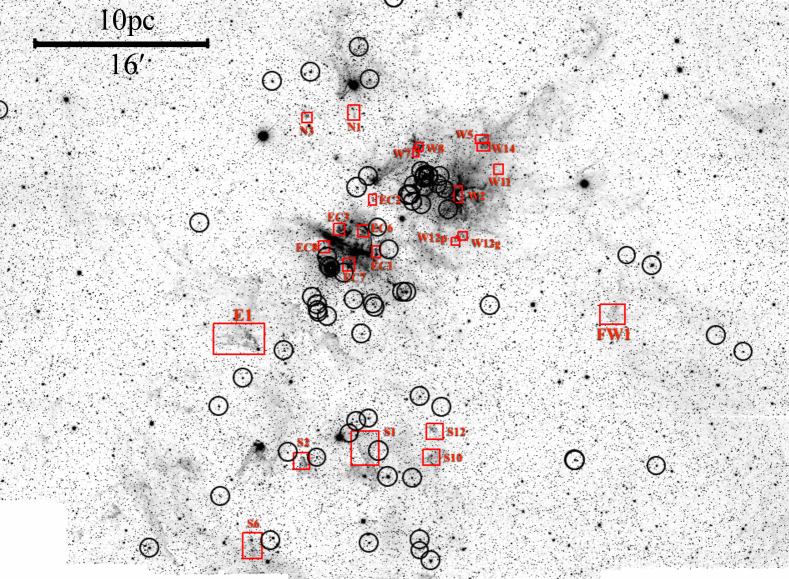
Figure 1: H₂ mosaic of Carina region from Hartigan et al. (2015). Irradiated molecular interfaces appear as the dark pillars and walls. The continuum has not been subtracted. The WR, O, and early B stars from Gagné et al. (2011) are shown in the black circles. The molecular cloud interfaces analyzed in this work are indicated by the red boxes. North is up and East is to the left in all the images.

2.1 Reduction

The near infrared (NIR) data used in this project were all taken with the NOAO NEWFIRM instrument. The imager consists of four 2048x2048 pixel detectors with a gap of 35 arcseconds between chips (Probst et al., 2008). Attached to the NOAO 4m telescopes, the imager has a pixel scale of 0.4 arcsec/pix. Details for the data acquisition for the three regions are given in Table 1. NEWFIRM has a data reduction pipeline (Swaters et al., 2009) that attempts a sky subtraction by using a median filter over the nearest 3 images in time before and after a frame is taken. As discussed in Hartigan et al. (2015), the pipeline is inadequate for regions of large-scale nebulosity. We therefore re-reduce the data in the manner outlined in Hartigan et al. (2015). To improve the S/N of our K-band mosaic, we used an archival NEWFIRM image of IC 1396A taken in 2009 by T. Megeath. This improved the S/N of the tip of IC 1396A significantly but did not help for regions further down the trunk. The maps of Carina were presented and thoroughly discussed in Hartigan et al. (2015), and several of the H₂ images of globules in Cygnus OB2 were shown in Hartigan et al. (2012).

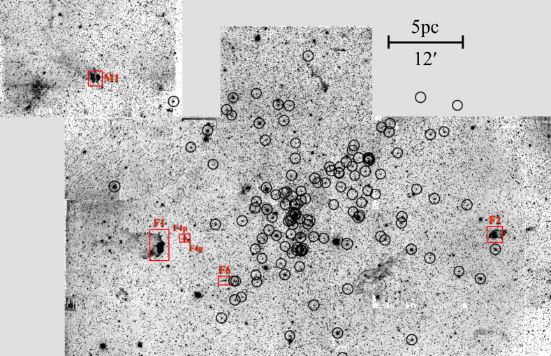
Figure 2: H₂ mosaic of Cygnus OB2 region. The location of the WR, O, and early B stars from Wright et al. (2015) are shown in the black circles. The molecular cloud interfaces analyzed in this work are indicated by the red boxes. The continuum has not been subtracted.

The final stacked results were then aligned between the three filters. S/N and exposure time varied within the frames due to the complicated dither patterns. The Carina data had average seeing of 1.09”, IC 1396 had 1.1”, and Cyg OB2 had 1.1”. The images were acquired through a variety of sky conditions and are not flux-calibrated, but this aspect does not affect the spatial offsets observed between H₂ and Br$\gamma$ emission or the spatial profile of either line, which are the focus of this paper.

2.2 Continuum Subtraction

The H₂ and Br$\gamma$ images are contaminated with continuum emission that arises primarily from starlight reflected from dust in the molecular clouds. We can remove the continuum by subtracting an appropriately scaled K-band image from both the Br$\gamma$ and H₂ mosaics. Because the wavelengths of H₂ (2.12$\mu$m) and Br$\gamma$ (2.17$\mu$m) are nearly identical and the continuum arises from the Rayleigh-Jeans part of the black-body spectrum for a usual star, the amount of continuum is nearly proportional to the bandpasses of each narrow-band filter. In this situation, there are three unknowns: the isolated H₂ and Br$\gamma$ emission and the pure continuum emission, and three constraints: the total emission recorded in each of the three filters. It is therefore possible to do filter “algebra” to isolate the line emission. In particular, we can write:

$$H_{2}^{tot}=H_{2}+\alpha K\\$$ (1)

$$Br\gamma^{tot}=Br\gamma+\beta K\\$$ (2)

$$K^{tot}=H_{2}+Br\gamma+K\\$$ (3)

where X^tot is the observed flux in the X-filter image and X is the contribution of the emission line. The constants $\alpha$ and $\beta$ are related through the bandpass widths of the H₂ and Br$\gamma$ filters, respectively. We determine their ratio empirically by constructing scaled subtractions between the H${}_{2}^{tot}$ and Br$\gamma^{tot}$ images. Stars will generally not have any line emission in H₂ or Br$\gamma$ and will subtract out with the correct values of $\alpha$ and $\beta$. We find that H${}_{2}^{tot}$ - $C\times$Br$\gamma^{tot}$, where $C\equiv\alpha/\beta$, optimally removes stars when $C$=1.19 for all regions in Carina and Cygnus except for one grid in Cygnus where $C$=1.40 is required. For IC 1396, $C$ was found to be between 0.85 and 1.05 depending on the region of the mosaic. The scaling factor includes the effects of different filter bandpasses, exposure times, and sensor sensitivities.

For some constant, $D$, adding $D$ times Eq. 2 to Eq. 1 and subtracting $D$ times Eq. 3 yields:

$$H_{2}^{tot}+DBr\gamma^{tot}-DK^{tot}=H_{2}(1-D)+K(\alpha+\frac{\alpha}{C}D-D)$$ (4)

When $D$ is chosen such that the stars are properly subtracted, we see that the coefficient of $K$ on the right hand side of Eq. 4 must be zero, implying:

$$\alpha=\frac{D}{\frac{D}{C}+1}$$ (5)

$\beta$ can then be found from the measured values of $C$. Once we know $\alpha$ and $\beta$, the line emission is given by:

$$H_{2}=\frac{H_{2}^{tot}-\frac{\alpha}{1-\beta}\times(K^{tot}-Br\gamma^{tot})}{1-\frac{\alpha}{1-\beta}}$$ (6)

$$K=\frac{K^{tot}-H_{2}-Br\gamma^{tot}}{1-\beta}$$ (7)

$$Br\gamma=Br\gamma^{tot}-\beta K\\$$ (8)

$\alpha$ and $\beta$ are slightly different for the different mosaics but always close to the ratios in bandpass between the H₂/Br$\gamma$ filters and the K filter. Our $\alpha$ and $\beta$ for Carina correspond very closely to those found by Yeh et al. (2015) who imaged 30 Dor with NEWFIRM.

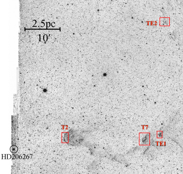
Figure 3: H₂ mosaic of IC 1396 region. Location of HD206267 in the center of Trumpler 37 is denoted by a black circle. IC 1396A, the Elephant Trunk nebula, is visible across the bottom of the frame pointing towards HD206267. Part of the edge of the cavity is visible in the upper right. The molecular cloud interfaces analyzed in this work are indicated by the red boxes. The continuum has not been subtracted.

3 Analysis

Our primary goal in this paper is to quantify how ionization fronts (IFs) and photodissociation regions (PDRs) appear in Carina, Cyg OB2, and IC 1396. In this section we summarize the general characteristics of the H₂ emission-line nebulae in each region (Section 3.1), investigate how the spatial profiles of Br$\gamma$ emission behave near the cloud surfaces (Section 3.2) and consider the observed spatial offsets between H₂ and Br$\gamma$ across the molecular cloud surfaces (Section 3.3). Our study quantifies differences in the size of this offset between the three star forming regions as well as trends in offset size with cloud geometry and irradiation environment.

3.1 The PDR Interfaces in Carina, Cyg OB2, and IC 1396

The H₂ images are excellent tracers of PDR interfaces, and reveal a variety of pillars, walls, and globules in Carina, Cyg OB2, and IC 1396 (Figs. 1-3). Each star-forming region has its own general character in the H₂ images. The image of Carina in Figure 1 contains several clusters, including Tr 14, the bright LBV star $\eta$ Car, and a wide variety of pillars, walls, and globules. In contrast, though Cyg OB2 also has large-scale H₂ walls, the brightest PDRs are associated with irradiated globules located in the vicinity of the concentration of massive stars in the middle of the images.

The last region, IC 1396A, is dominated by the Elephant Trunk Nebula, a long pillar structure. Also present are the edges of a large, circular bubble surrounding Tr 37. Because of the low S/N of the K-band image, we focus primarily on the PDR interfaces along and at the base of the trunk where the S/N is the best in the K-band. In all of our regions the Br$\gamma$ emission is located closer to the ionizing sources than the H₂, compatible with the picture of molecular clouds being ionized and dissociated by radiation from the newborn stars. For many of the bright interfaces, streams of photoionized gas are visible in Br$\gamma$ as they evaporate from the surface of the clouds.

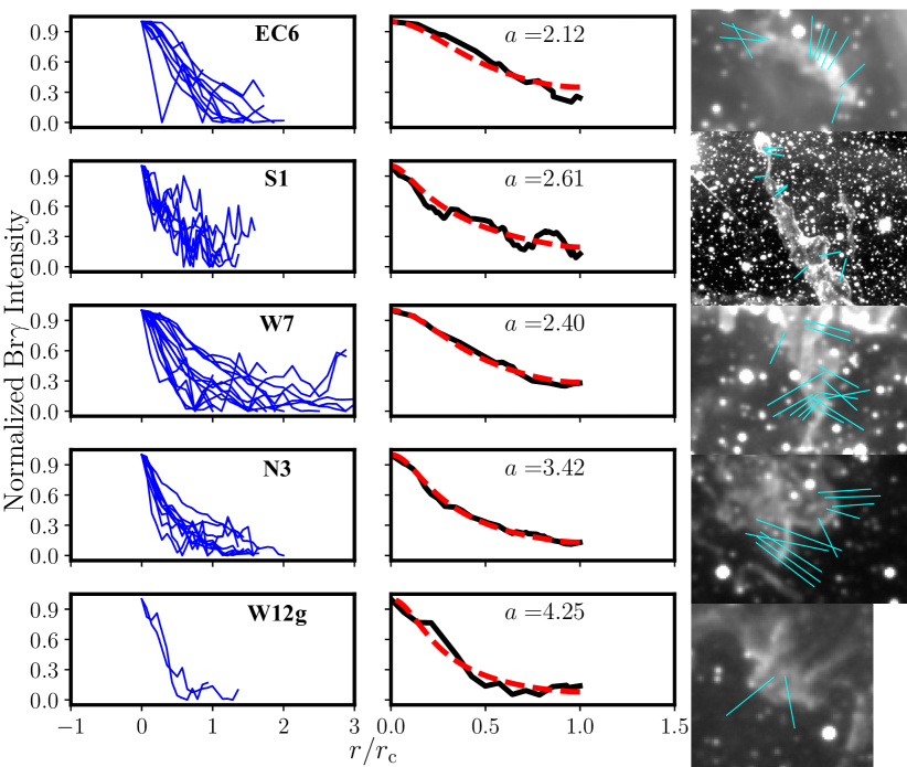
Figure 4: Continuum subtracted Br$\gamma$ profiles for five PDR interfaces in Carina. The left column shows all Br$\gamma$ profiles for a given interface. The middle column shows the median profile shape along with the best power-law fit. The right column displays an H₂ image of the object (not continuum-subtracted) together with the locations of all the slices (shown in blue) that were used to fit the Br$\gamma$ profiles. The labels of the interfaces, as listed in the appendix, are indicated in the upper left.

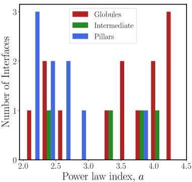
Figure 5: Histogram of power law indices for 26 different interfaces in Carina and Cyg OB2, broken into groups by their approximate geometric shape.

3.2 Br$\gamma$ Profiles and Interface Shapes

We can study the IFs and photoevaporative flows in these regions by measuring the spatial profiles of Br$\gamma$ intensity near the surface of the clouds. Br$\gamma$ emission arises from photoevaporative flows off of the cloud. Its brightness should reflect the density profile of the flow because Br$\gamma$ emissivity $\propto n_{e}n_{p}$. Photoevaporative flows ablate from cloud surfaces at a few times the sound speed (Bertoldi, 1989). If we assume that the flow moves with a roughly constant velocity then conservation of mass requires that the density falls like $n\propto r^{-2}$ for spherical clouds and $n\propto r^{-1}$ for cylindrical clouds, where $r$ is the distance from the surface of the cloud. Assuming that the transition from neutral to ionized material is over a short distance, we then expect the Br$\gamma$ emissivity to follow a power law profile of the form:

$$\epsilon_{\rm Br\gamma}\propto\left(\frac{r+r_{c}}{r_{c}}\right)^{-b}$$ (9)

where $r$ is the distance along the profile with $r=0$ corresponding to the peak in Br$\gamma$ emission at the cloud’s surface, $r_{c}$ is the radius of curvature of the cloud, and $b=2$ for a pillar and $4$ for a globule. Assuming that the photoevaporative flow extends outward from the cloud’s surface to infinity, projecting the Br$\gamma$ emissivity (Equation 9) onto the plane of the sky yields an observed Br$\gamma$ intensity profile of the form:

$$I_{\mathrm{Br\gamma}}=I_{\mathrm{max}}\left(\frac{r+r_{c}}{r_{c}}\right)^{-a}$$ (10)

where $I_{\rm max}$ is the peak Br$\gamma$ intensity on the profile and $a=b-1$. In other words, the effect of projection on the Br$\gamma$ profile is to make the power law shallower, decreasing the power law exponent by one, regardless of whether it is a pillar or globule. In the more realistic case that the photoevaporative flow does not extend to infinity and a uniform background takes over at some distance from the cloud, the projected intensity profile will not strictly be a power law since it goes to a constant at some radius. Assuming that the flow extends out at least a few times the radius of curvature of the cloud from the cloud’s surface, the profile can be approximated as a power law with the exponent in between the unprojected and infinite flow cases. This means that we expect globules to have roughly power law Br$\gamma$ intensity profiles with exponent in between $-3$ and $-4$ and pillars to have exponents between $-1$ and $-2$.

To compare this with our data, we extract slices from the continuum-subtracted Br$\gamma$ images across cloud interfaces. Slices were taken only on interfaces that appear edge-on, and we averaged the profiles over 5 pixels perpendicular to the slice to improve S/N. Slices must exclude stars, and this requirement limits the total number of slices. Slices were taken on a variety of interfaces, including pillars, walls, and globules. For a given interface, we extracted several independent slices and aligned them by using the peak Br$\gamma$ emission. These slices generate a median profile shape for each interface. Only the part of the slices on the HII region side of the Br$\gamma$ peak is kept for this analysis. To isolate the Br$\gamma$ emission in the photoevaporative flow from foreground/background nebulosity, a background level is subtracted from each slice. The background is quantified as the minimum pixel value along the slice. To make sure that the slices extend far enough out into the HII region that this minimum value does represent a background level and is not due to the photoevaporative flow itself, we further restrict slices to be longer than the radius of curvature of the object. We grouped interfaces into three broad categories: globules, which have roughly spherical symmetry; pillars, which have approximately cylindrical symmetry; and intermediate shaped clouds, which are a mixture of the two. The pillars are specifically defined as those objects with a long axis being at least twice the length of a short axis. For all the interfaces we can estimate a radius of curvature directly from the H₂ images by fitting an arc with a constant radius of curvature to the feature. The profiles were fit in the range $r=0$ to $r=r_{c}$. To account for the blurring effect of seeing, the profile of Equation 10 is first convolved with a Gaussian of the width of the seeing before being fit to the data.

Figure 4 shows these fits for five typical interfaces in Carina. The middle column shows the median profile shape and the best fitting power-law. Images of the interfaces are also shown. The top two interfaces are categorized as ‘pillars’, the middle one as ‘intermediate’, and the bottom two as ‘globules’. The power law slope is steeper for the globules than the pillars, as expected, because the extra curvature in the globules causes the gas to diverge over shorter spatial scales than in the pillars. Doing this analysis for 26 objects in Carina and Cygnus OB2 we derive the power law fits shown in Figure 5. The ‘globule’ interfaces have an average power law index of $-3.45\pm 0.22$ whereas the ‘pillar’ interfaces have an average index of $-2.54\pm 0.16$. A two sample $t$-Test indicates that these means are significantly different with a $p$-value of 0.004. The globule power law exponents agree well with the expectation above that they fall in between $-3$ and $-4$, and the globule objects have steeper profiles than the pillars, also consistent with simple theoretical expectations. The power law exponents for the pillars are likely greater than the expected values between $-1$ and $-2$ because the objects are not exclusively cylindrical but consist of a mixture of cylindrical and spherical curvature. A list of all the interfaces considered can be found in Appendix A

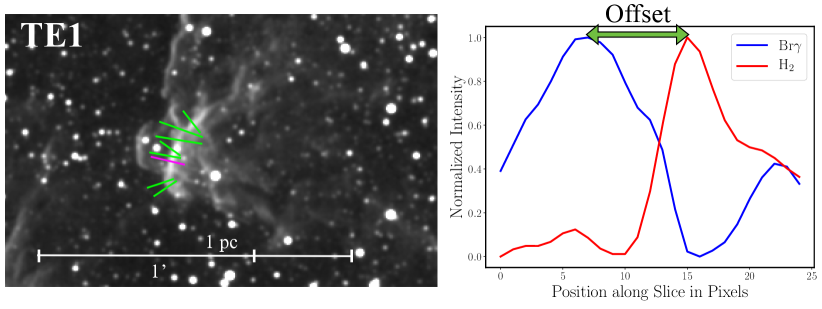
Figure 6: H₂ image (not corrected for continuum) of one of the objects in IC 1396 used for measuring spatial offsets between H₂ and Br$\gamma$ emission. The green lines mark locations where the continuum-corrected spatial profiles were extracted for the emission lines. The spatial offset between H₂ and Br$\gamma$ is shown at right for the position defined by the purple line. The interface’s label, as given in the appendix, is indicated in the upper left.

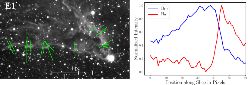
Figure 7: Same as Figure 6 for an object in Carina.

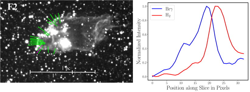
Figure 8: Same as Figure 6 for an object in Cygnus OB2.

3.3 Spatial Offsets Between H₂ and Br$\gamma$

As noted in Hartigan et al. (2015), there is a distinct offset between the H₂ and Br$\gamma$ emission when slices are extracted across PDR interfaces. Since the H₂ and Br$\gamma$ lines are so close in wavelength, this offset should be independent of extinction, and it should reflect the physical size of the PDR and ionization front. In this section we quantify this offset in Carina, IC 1396, and Cyg OB2. Sample slices for each of the three regions are shown in Figs. 6-8, displaying typical offsets between H₂ and Br$\gamma$ for irradiated clouds.

Because the three star formation regions we are analyzing are at different distances, the images will have markedly different spatial resolutions even if the seeing were the same. To correct for this effect, we bin the IC 1396 and Cygnus OB2 data so that they have the same pixel scale as the Carina data (Carina is the furthest region of the three). We assume a distance of 1400 pc to Cyg OB2 (Rygl et al., 2012), 2300 pc to Carina (Smith, 2006), and 870 pc to IC 1396 (Contreras et al., 2002). At the distance of Carina, one pixel corresponds to $1.38\times 10^{16}$cm. To equalize the seeing, we blurred all the data down to the level of the image with the worst seeing by convolving the images with Gaussians of varying widths. The image with the worst seeing is the K-band Carina image with a FWHM seeing of $3.95\times 10^{16}$cm (at the distance of Carina), and all final images have this same level of smoothing.

To quantify the observations we simply measure the spatial offset between the peak emission in Br$\gamma$ and in H₂ in the smoothed images. Since the slices do not need to be longer than the interface’s radius of curvature, we can consider more distinct objects than in Section 3.2. In total, we consider 33 objects across the three regions consisting of around 450 distinct slices. These objects are listed in Appendix A.

Figure 9 shows the cumulative distribution for physical offset sizes for the three regions. IC 1396 appears to have the largest offsets while Cyg OB2 and Carina have roughly similar offsets. IC 1396 has median offset size of $9.9\times 10^{16}$cm, while Carina has median offset size of $7.9\times 10^{16}$cm, and Cyg OB2 has median offset of $7.8\times 10^{16}$cm. Figure 9 shows that the offsets are all within roughly a factor of two of $10^{17}$cm, despite the fact that the three regions span at least three orders of magnitude in the intensity of ionizing radiation.

We can use our data to determine if the observed offsets depend upon the radius of curvature of the cloud or the strength of the radiation field. Many interfaces have approximately spherical or pillar-shaped morphologies, while others appear intermediate between these shapes. The H₂ image gives a characteristic radius of curvature for each interface, with a typical error of $\pm$ 10%. To estimate the intensity of ionizing radiation incident onto each interface, we use catalogs of the O and early B-type stars in the regions. For Carina, we reference the catalog of O/B stars compiled by Gagné et al. (2011), and for Cygnus OB2, we apply the list of Wright et al. (2015). Because HD 206267 is the lone O-star in IC 1396, we need only consider that source. We convert the spectral type to ionizing photon output using values from Martins et al. (2005). To approximate the flux of ionizing photons incident at each slice location, we consider only the O/B stars that are visible to that slice in the direction above the cloud interface. We combine the stars via:

$$F=\sum_{i}\frac{Q_{i}\cos(\theta)}{4\pi r^{2}},$$ (11)

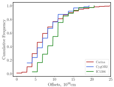
Figure 9: Distribution of offset sizes.

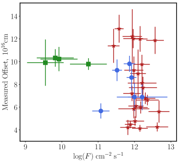
Figure 10: Measured offset sizes versus the estimated incident flux of H-ionizing photons. Objects in Carina are shown in red, those from Cygnus OB2 are in blue, and those from IC 1396 are in green. The flux of ionizing photons spans three orders of magnitude.

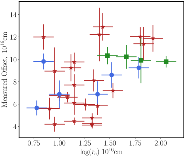
Figure 11: Measured offset sizes versus the measured radius of curvature. Objects in Carina are shown in red, those from Cygnus OB2 are in blue, and those from IC 1396 are in green.

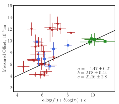
Figure 12: Edge-on view of best fitting plane to the measured offset values along with best-fitting parameter values. Objects in Carina are shown in red, those from Cygnus OB2 are in blue, and those from IC 1396 are in green.

where $Q_{i}$ is the ionizing photon output of the $i$-th star, $\theta$ is the angle between the line connecting the star to the interface and the normal to the interface (which is taken to be the slice we make), and $r$ is the projected distance between the star and the interface.

To account for projection effects, we calculate an uncertainty in the flux, $F$, by assuming that the distance, $r$, is known to within 25%. This uncertainty is then propagated through to the final flux value for each slice. We average the flux values for each slice on an object to get an estimate for the flux value for that object. Since the uncertainties for the flux value at each slice on an object are not uncorrelated, we just take the rms of these uncertainties as an estimate for the uncertainty in the ionizing flux for that object. It is also possible to estimate the FUV flux at each point in the regions from the observed far-infrared (FIR) intensities (e.g. Kramer et al., 2008; Roccatagliata et al., 2013) but since the EUV flux is more relevant to studying the IFs and photoevaporative flows, we do not explore that method here.

The offsets measured from slices on an object are averaged to give a mean offset for that object and a standard error of the mean.

After these measurements are completed, each object has an associated radius of curvature, an ionizing flux level, and a spatial offset between Br$\gamma$ and H₂. Figure 10 shows the measured offsets as a function of the estimated incident flux. The range in $\log(F)$ shows that our objects differ in the level of incident flux by around three orders of magnitude between the weakest irradiation environment in IC 1396 and the strongest in Carina. Figure 11 shows the offsets as a function of the measured radius of curvature. There is a reasonably strong positive correlation between the offset size and the radius of curvature and a very weak negative correlation with respect to the incident flux. A Spearman rank-order test for Figure 10 gives a $p$-value of no correlation of 0.05 and a $p$-value of 0.007 for Figure 11. The low $p$-value in Figure 10 is probably driven by the IC 1396 interfaces at low incident flux. Not including the IC 1396 interfaces yields $p$-values of 0.3 and 0.07 for Figures 10 and 11, respectively. Both Figures 10 and 11 show a significant spread in the offset sizes even after all the individual slices for an object have been averaged. Each point in Figures 10 and 11 is already an average of 10-20 individual slices.

The spatial offsets between Br$\gamma$ and H₂ should depend jointly upon both the incident flux and radius of curvature, which introduces scatter to Figures 10 and 11 when offsets are plotted against either $\log(F)$ or $\log(r_{c}$) individually. To correct for this effect, we fit a plane to the offset values of the form:

$$\mathrm{O}=a\log(F)+b\log(r_{c})+c$$ (12)

where $\mathrm{O}$ is the measured offset. Figure 12 shows an edge-on view of this plane along with the best fit parameters $a,\;b,$ and $c$. The scatter in the planar view (Figure 12) is less than that for $\log(F)$ (Figure 10) and for $\log(r_{c})$ (Figure 11), though considerable intrinsic scatter remains, caused in large part by the complex geometrical shapes of the individual objects and uncertainties in the true (deprojected) distances of the ionizing sources from the cloud interfaces. Nevertheless, there is a weak positive trend, $b=2.08\pm 0.44$, of the offsets with radius of curvature of the cloud and a weak negative trend for the offset with the incident flux, $a=-1.47\pm 0.21$.

4 Photoionization Models

4.1 Motivation

Our two primary motivations for developing a numerical model of these regions are (1) to explain the differences and similarities in the offset sizes observed in the three regions and (2) to explore the relevant physical processes that define the size of the offsets. The fact that the three regions show similar offsets indicates that offsets might end up being more useful as a rough distance indicator than as a PDR diagnostic tool. Hence, rather than use the spatial offset between Br$\gamma$ and H₂ to determine physical conditions, the focus will be to understand the underlying processes that create these offsets and to predict any correlations with other observables.

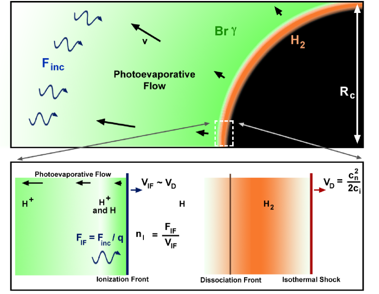
Figure 13: Schematic of a photoevaporative flow from an irradiated globule. Top: Ionizing flux $F_{\rm inc}$ from the left impinges upon a dense spherical globule of radius $r_{c}$ and drives an outflow. The green colors depict Br$\gamma$ emission and the red show H₂ emission. Bottom: Recombining gas in the outflow reduces the incident ionization flux by a factor of $q$ at the ionization front. The ionization front progresses into the cloud at a velocity $v_{\rm IF}$ $\sim$ $v_{D}$, where $v_{D}$ is the velocity of the isothermal D-shock, set by the sound speeds $c_{i}$ and $c_{n}$ in the ionized and neutral gases, respectively. The model solves ionization and dynamical equations for $q$ to determine $n_{\rm I}$, which in turn becomes an input parameter to Cloudy for determination of the H₂ emission. The velocity arrows depicted in the figure are relative to the unperturbed globule.

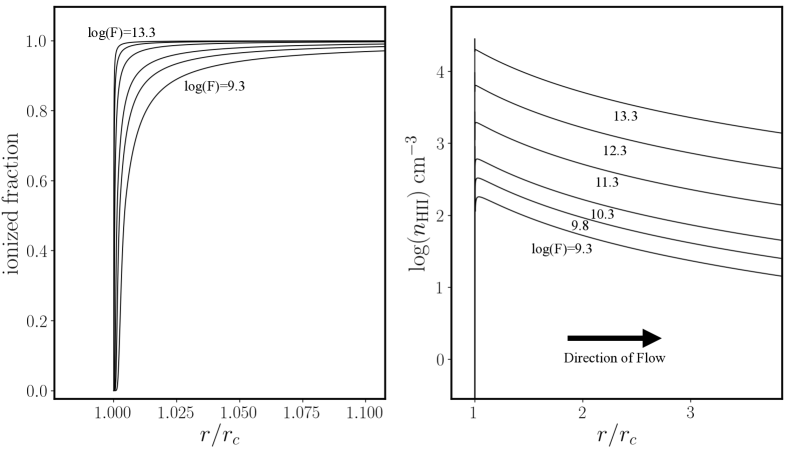
Figure 14: Model results for models with $r_{c}=5\times 10^{17}$cm. The left plot shows profiles of the ionization fraction. The right plot shows the electron number density for the same models. In order of increasing ionization fraction at a given radius, the models have $\log(F)=9.3,9.8,10.3,11.3,12.3,13.3$ cm^-2s^-1.

4.2 Model of a Photoevaporative Flow

The Br$\gamma$ emission originating near the molecular clouds comes from a photoevaporative flow of ionized gas off the cloud surface. Therefore, to accurately model the offsets and their dependence on various parameters, a rough model of a photoevaporative flow is necessary. We follow Bertoldi (1989) and solve the equations of hydrodynamics and ionization balance in a simplified spherically symmetric, 1-D geometry and in the steady-state. In this formalism, all partial time derivatives in the fluid equations are set to zero. A picture of the physical situation along with a definition of the variables is shown in Figure 13. We solve the continuity equation, momentum equation, and equations for ionization balance as:

$$\frac{d}{dr}\left(r^{2}n_{\rm H}v\right) =0$$ (13)

$$v\frac{dv}{dr} =-\frac{1}{\rho}\frac{dP}{dr}$$

$$\frac{dF}{dr} =(1-x)n_{\rm H}\sigma_{\nu}F$$

$$\frac{dx}{dr} =\frac{1}{v}\left(-\alpha_{b}x^{2}n_{\rm H}+(1-x)\sigma_{\nu}F\right)$$

where $n_{\rm H}$ is the hydrogen number density, $\rho=m_{\rm H}n_{\rm H}$, $P$ is the pressure, $v$ is the velocity of the flow, $F$ is the flux of ionizing photons at a certain point in the flow, $x$ is the ionization fraction, $\alpha_{b}$ is the case-B recombination coefficient, and $\sigma_{\nu}$ is the frequency averaged photoionization cross section for hydrogen. We use $\alpha_{b}=2.7\times 10^{13}$cm³s^-1 and $\sigma_{\nu}=3.0\times 10^{-18}$cm². Following Lefloch & Lazareff (1994), instead of solving a separate energy differential equation, we write the sound speed as:

$$c^{-2}=c_{i}^{-2}+\left(c_{n}^{-2}-c_{i}^{-2}\right)\left(1-\sqrt{x}\right)^{2}$$ (14)

which is essentially an arbitrary interpolation function between the two extremes, $c_{n}$ and $c_{i}$, the isothermal sound speeds for the cold neutral gas and the warm ionized gas, respectively. We take $c_{n}$ = 0.8 km/s corresponding to $T=100$ K neutral hydrogen and $c_{i}$=11.4 km/s corresponding to $T=10^{4}$ K ionized hydrogen. As discussed in Lefloch & Lazareff (1994), writing the sound speed explicitly as such requires that the flow be in thermal equilibrium. More specifically, it requires that the thermal timescale be much less than the dynamical timescale of the flow. Lefloch & Lazareff (1994) argue that this is the case for flows with strong irradiance where the flow acts as an insulating boundary layer and absorbs most of the incoming ionizing photons before they reach the IF. This will be the case for the regions we consider with strong irradiance in Carina and Cygnus but might not be accurate for the objects in IC 1396 which have fairly weak incident radiation.

We assume the ionization front is D-type and is therefore preceded by a shock wave in the steady-state (Figure 13). Following Bertoldi (1989) we model the flow from the neutral part outwards. Bertoldi (1989) found that the velocity of the IF is approximately the D-critical velocity under a wide range of conditions. We write the IF velocity as

$$v_{\rm IF}=\phi_{d}v_{D}$$ (15)

where $v_{D}$ is the D-critical velocity $\approx c_{n}^{2}/2c_{i}\approx 0.03$ km/s (Spitzer, 1968) and $\phi_{d}$ is an order unity number. We will assume that $\phi_{d}=1$. Additionally, the density of the shocked gas layer will be

$$n_{\rm I}=\frac{F_{\rm IF}}{v_{\rm IF}}$$ (16)

where $F_{\rm IF}$ is the flux of ionizing photons that actually reaches the IF. We parameterize the effect of shielding by the flow by writing $F_{\rm IF}=F_{\rm inc}/q$ where $q$ is unknown a priori and $F_{\rm inc}$ is the incident flux. The model starts in the neutral part of the cloud with $F_{0}=10^{-8}F_{\rm inc}$ and $x_{0}=10^{-8}$ and numerically integrates the equations as it moves outwards. The gas accelerates as it heats up and becomes super-sonic. However, since we are interested in the density profiles near the IF and not further out along the flow, we do not follow the super-sonic evolution. Once the gas becomes faster than $0.99$ times the sound speed, we set the gas velocity as the sound speed and do not consider the momentum equation any further. This allows us to avoid the complication that the momentum equation is actually singular at the sonic point. The models are integrated from $1r_{c}$ to $5r_{c}$. The parameter $q$ is chosen so that the flux at $5r_{c}$ is within 5% of the intended incident flux, $F_{\rm inc}$. We repeat the process for various radii of curvatures and fluxes relevant to our regions. Ionization fraction and density profiles for models with $r_{c}=5\times 10^{17}$cm for a variety of incident ionizing fluxes are shown in Figure 14.

The models show a spike in the density of HII in the profiles in the ionization fronts. This occurs because there is a large density contrast across the IF of roughly a factor of $c_{i}/v_{\rm IF}\approx 200$. This causes the IF to have higher density than the photoevaporative flow and so even if the IF is not completely ionized, it can have a higher HII density than in the flow. This spike is model dependent (it is sensitive to our simplified energy equation) and it is unclear if it would be present if heating and cooling are explicitly considered. We do not consider this here as the spike is too narrow to affect the observed offset between Br$\gamma$ and H₂. It will be completely smoothed once blurred by the seeing.

Figure 15 shows the scalings of the maximum HII density in the flow with the flux and radius of curvature. Also shown is the expectation for a flow with constant velocity and infinitely thin IF given by (e.g. Tielens, 2005):

$$n_{\mathrm{HII,\;max}}=\left(\frac{3F}{r_{c}\alpha_{b}}\right)^{1/2}$$ (17)

This density is found by assuming that the photoevaporative flow acts as an insulating boundary layer that absorbs most of the ionizing photons before they reach the IF. We can see that the scalings in the simulations with regard to $F$ and $r_{c}$ are the same as Equation LABEL:eq:ana but that the simulation densities are roughly $1.5\times$ higher. This is due to the fact that the ionization fronts have non-zero thickness. Equation LABEL:eq:ana assumes that all of the ionized hydrogen lies outside the IF and moves at a constant velocity where, in our models, the peak density of HII occurs inside the IF where gas is not completely ionized but is very dense because the gas is still moving slowly. As mentioned above, conservation of mass requires that the density of the gas before the IF is roughly $\approx 200$ times that of the gas on the ionized side of the IF. Within the IF, the gas density will be somewhere in between.

This scaling of $n_{\mathrm{HII,\;max}}\propto F^{1/2}$ is found to agree quite well with the pillar mass loss rates in Carina, M16, and NGC 3603 analyzed in McLeod et al. (2016).

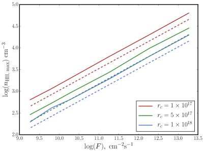
Figure 15: Solid lines show the maximum HII density in the simulations as a function of $F$ and $r_{c}$. In dotted lines is shown the expectation for a photoevaporative flow with constant velocity and infinitely thin IF (cf. Equation LABEL:eq:ana).

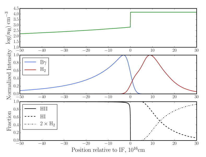
Figure 16: Sample model result with $r_{c}=5\times 10^{17}$cm and $F=10^{10.2}$cm^-2s^-1. The profiles are centered on the ionization front defined as where the ionization fraction is 50%. Note that we do not see a rise in the neutral HI fraction right after the IF because this is where the dynamical model stops and the Cloudy model begins. The Cloudy model starts with the HI fraction being $1$.

4.3 Synthetic Br$\gamma$ and H₂ Spatial Line Profiles

Synthetic observations play a key role in interpreting real observations. For a recent review of applications of synthetic observations, see Haworth et al. (2018). In this investigation, we generate synthetic spatial emission profiles from the photoevaporative flow models described above. We create the profile for each line separately and then stitch them together. To create the Br$\gamma$ profile, we simply square the HII density profile calculated in the model. Because we are not interested in the actual Br$\gamma$ emissivity, we do not need to worry about the recombination coefficient. In doing this, we ignore the dependence of the recombination coefficient on the temperature but that is a minor effect compared to the variations in HII density.

To create the H₂ profile, we use the photoionization code Cloudy, version 13.03, described by Ferland et al. (2013). Cloudy works by providing it a density law and input spectrum and it does the necessary radiative transfer to predict the H₂ emissivity. Bertoldi & Draine (1996) found that, after a transitory initial phase, the dissociation front (DF) is trapped within the shocked layer. This means that the PDR, where the HI exists and where the 2.12$\mu$m emission is coming from, is situated in the shocked layer. Hence, we model the PDR in Cloudy by assuming a constant density of $n_{\rm I}$ found from the dynamical models. The shape of the input spectrum is that of an O6 star from the TLUSTY stellar atmosphere models (Hubeny & Lanz, 1995) with all of the Lyman continuum photons removed. This is only an approximation as the photoevaporative flow will modify the spectrum more than just extinguishing the Lyc photons, however it should be enough to understand general trends in the offsets.

The models are also approximate in the sense that Cloudy does static modeling but the PDR is actually evolving as hydrogen advects across it at the speed of the dissociation front. Bertoldi & Draine (1996) find that non-equilibrium effects in the PDR, including transient photochemistry, are important when the incident flux and the density of the cloud is low. From their Figure 4, the regions we consider that have strong incident flux like that characteristic of Carina and Cygnus should be well-matched with equilibrium PDR models (like Cloudy) though objects with weaker incident flux like in IC 1396 might not be. Despite this limitation, we use Cloudy to get a rough understanding of the general trends in the offsets. The models run deep into the molecular region of the clouds, and we adopt Cloudy’s default chemical abundances for an HII region, which are average values of the abundances in the Orion Nebula Rubin et al. (1991); Baldwin et al. (1991); Osterbrock et al. (1992); Rubin et al. (1993), with a metallicity of 0.4 solar. The models also include dust grains with the size distribution and abundances of grains found in the Orion Nebula. Additionally, the models include a cosmic ray flux characteristic of the galactic background taken from Indriolo et al. (2007). We combine the two profiles together simply by stitching the H₂ profile onto the location where the dynamical models begin (with $F_{0}=10^{-8}F_{\rm inc}$ and $x_{0}=10^{-8}$) . Both the Br$\gamma$ and H₂ profiles are then blurred to the same level of seeing as the NIR images by convolving them with the appropriate Gaussian. A sample model result is shown in Figure 16. The density profile shows the $1/r^{2}$ fall-of in the photoionized flow, the large density contrast across the IF, and the constant density through the PDR. The offset is then easily measured as the distance between the peak Br$\gamma$ and H₂ emission.

Finally, it is worth noting that the models are 1D whereas the real objects are 3D and so these spatial profiles will not capture the effects of projecting the 3D emission profiles along the line of sight. This will have the effect of blurring out the profiles since sight lines will probe ionized material at different locations in the photoevaporative flow and neutral material. However, since the radii of curvature of the objects we consider are generally $\gtrsim 5$ times the offset size, the effect of projection along the line of sight will be relatively small on the measured offset size. Accurately projecting along the line of sight would require a radiative transfer calculation of the H₂ through the pillar which is beyond the scope of the current project. For other successful examples of using 1D models to interpret observed spatial line profiles in photo-evaporative flows, see, e.g., Sankrit & Hester (2000); McLeod et al. (2016). However, 1D models might lead to erroneous interpretations of spatially resolved line ratios as discussed in Ercolano et al. (2012).

Figure 17 shows the results of these models for a variety of values of $r_{c}$ and $F$. The model offsets always lie within roughly a factor of two of $10^{17}$cm even over a wide range in parameters, in agreement with the observations. With the exception of the left edge, the offsets decrease with increasing $F$ and decreasing $r_{c}$. This trend arises from the increase in density in the shocked layer that occurs by increasing $F$ or decreasing $r_{c}$ (see Figure 15). Increasing the density leads to a thinner PDR because the thickness of the PDR is set by the column density of hydrogen and a thinner PDR leads to a smaller offset. The decrease in offsets for log(F) $\lesssim$ 10.4 in Figure 17 is caused by the incident radiation being so weak that a distinct layer of HI is not formed in the Cloudy models and so the H₂ emission comes from very close to the IF and the offset declines. At these low incident fluxes, the static models of the PDR are probably inadequate as the advection of hydrogen through the PDR will start to matter (Bertoldi & Draine, 1996). It is possible for the ionization and dissociation fronts to merge under certain conditions (e.g. Störzer & Hollenbach, 1998; Henney et al., 2007), however our static models are certainly inadequate to describe this situation.

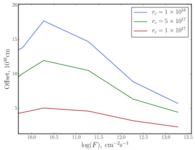
Figure 17: Predicted model offsets between Br$\gamma$ and H₂ for different radii of curvature and incident fluxes.

5 Conclusions

In this work, we present sky-subtracted large-scale mosaics in H₂ and Br$\gamma$ for three regions of massive star formation: Cyg OB2, Carina, and IC 1396. The three regions span roughly three orders of magnitude in ionizing flux and so provide a powerful means to investigate the physics that underlies the spatial profiles and offsets we observe in the dozens of PDR fronts that populate these regions.

Each of the three star forming regions contains PDRs that have a wide variety of geometrical shapes, ranging from more or less spherical globules to highly-elongated cylindrical pillars. To understand how the shapes of the interfaces affect what is observed in the images, we fit power laws to the spatial profiles of continuum-corrected Br$\gamma$ flux along several hundred lines of sight and grouped the results according to the overall shapes of the irradiated interfaces. The results confirm model predictions that the shape of the object strongly influences the spatial profile of the emission in a photoevaporative flow. Br$\gamma$ fluxes from cylindrically-shaped clouds have a relatively flat radial power law index of $-2.54\pm 0.16$, while spherically-shaped clouds decline more rapidly with distance, with an average power-law index of $-3.45\pm 0.22$. The globule power-law exponents agree well with the expected values between $-3$ and $-4$, although the pillar power-law exponents are somewhat higher than the expected values between $-1$ and $-2$, predicted for photoevaporative flows of constant velocity. Broadly speaking, the results are consistent with model expectations that more spherical clouds should exhibit sharper radial decline in the Br$\gamma$ emission as compared with cylindrical clouds.

We observe spatial offsets between the peaks of the H₂ and Br$\gamma$ emission throughout each of the three star formation regions, always in the sense that the H₂ emission is located deeper into the molecular cloud, underneath a layer of Br$\gamma$ emission that traces a photoevaporative flow. By extracting several hundreds of slices across a wide variety of distinct PDR interfaces, we found that the spatial offsets between these two lines are always on the order of $10^{17}$ cm for all the objects in all three regions.

After estimating the incident ionizing flux, $F$, received by each object and measuring an approximate radius of curvature $r_{c}$ for each object, we investigated how these two variables correlate with the observed spatial offsets between Br$\gamma$ and H₂. There is a significant increase in the spatial offset as $r_{c}$ increases. A weak trend of decreasing offset with $F$ is also observed. Individual geometrical complications introduce significant scatter to these trends.

To investigate the physical processes that determine why the offsets form and what sets their sizes, a simple theoretical model of Br$\gamma$ emission from a photoevaporative flow is developed by solving the time-independent Euler and ionization equations. These density profiles are then used in the numerical code Cloudy to predict synthetic spatial line profiles for the H₂ emission. The models reproduce all the main results in the data, including the size of the spatial offsets between H₂ and Br$\gamma$, the positive correlations of the offsets with the radius of curvature of the object, and even the weak negative correlation of the offset with the amount of incident ionizing flux.

Overall, these observations support the general picture of molecular clouds being photoevaporated by young massive stars and lend some confidence that the basic physics that underlies these systems is understood. However, it is clear that the geometries of the interfaces can be very complex, and this complexity has a significant effect upon what is observed. Both the H₂ and Br$\gamma$ lines will be easily observable at high spatial resolution in PDRs with the James Webb Space Telescope, and all of the analyses done here will be possible to extend to much smaller spatial scales as long as continuum images are also acquired to enable accurate background subtraction of the ambient reflected starlight.

Appendix A List of Objects

The specific interfaces analyzed are listed below along with various calculated parameters.

Table 2: List of interfaces analyzed. $a$ is the best-ftting (negative) log slope of the Br$\gamma$ profile, $r_{c}$ is the estimated radius of curvature, and $\log(F_{\rm inc})$ is the calculated incident flux of ionizing photons at the location of the interface from the O/B stars in the region. Regions with no entry for $a$ are regions that were not included in the analysis of Section 3.2 because slices longer than the radius of curvature could not be found but were included in the analysis of Section 3.3.

Object	Region	RA	Dec	$a$	$r_{c}$, $10^{16}$cm	$\log(F_{\rm inc})$, cm-2 s-1	Average Offset, 1016 cm	Number of Slices	Morphological Type
E1	Carina	10:46:00	-59:47:30	2.80	87.0$\pm 8.7$	11.96$\pm 0.27$	12.02$\pm 0.84$	19	Pillar
EC1	Carina	10:44:31	-59:39:50	2.60	13.8$\pm 1.4$	12.30$\pm 0.28$	6.78$\pm 0.51$	13	Globule
EC2	Carina	10:44:33	-59:34:57	3.76	16.6$\pm 1.7$	12.36$\pm 0.31$	6.62$\pm 0.46$	26	Intermediate
EC3	Carina	10:44:57	-59:37:25	3.55	17.9$\pm 1.8$	11.98$\pm 0.26$	9.24$\pm 1.20$	7	Globule
EC6	Carina	10:44:40	-59:37:52	2.12	9.7$\pm 1.0$	12.15$\pm 0.20$	11.99$\pm 1.12$	14	Pillar
EC7	Carina	10:44:51	-59:40:51	3.95	19.3$\pm 1.9$	12.20$\pm 0.22$	9.76$\pm 0.84$	11	Intermediate
EC8	Carina	10:45:08	-59:39:14	3.98	19.3$\pm 1.9$	12.23$\pm 0.39$	7.71$\pm 0.96$	10	Globule
FW1	Carina	10:41:46	-59:45:14	–	93.8$\pm 9.4$	11.43$\pm 0.16$	11.39$\pm 1.49$	11	Globule
N1	Carina	10:44:47	-59:27:22	2.19	12.42$\pm 1.2$	11.82$\pm 0.21$	4.20$\pm 0.66$	17	Pillar
N3	Carina	10:45:20	-59:27:36	3.42	19.3$\pm 1.9$	11.89$\pm 0.15$	4.47$\pm 0.33$	12	Globule
S12	Carina	10:43:50	-59:55:23	2.04	34.5$\pm 3.5$	11.94$\pm 0.27$	12.21$\pm 2.39$	8	Pillar
S10	Carina	10:43:53	-59:57:59	2.41	46.9$\pm 4.7$	11.93$\pm 0.24$	7.20$\pm 0.67$	13	Globule
S1	Carina	10:44:40	-59:57:33	2.61	30.4$\pm 3.0$	12.21$\pm 0.39$	8.11$\pm 0.98$	19	Pillar
S2	Carina	10:45:23	-59:58:19	3.25	33.1$\pm 3.3$	11.98$\pm 0.43$	5.85$\pm 0.83$	8	Intermediate
S6	Carina	10:45:59	-60:05:49	2.47	37.3$\pm 3.7$	11.58$\pm 0.12$	12.89$\pm 1.2$	19	Pillar
W11	Carina	10:43:06	-59:32:13	2.34	24.8$\pm 2.4$	12.17$\pm 0.19$	5.96$\pm 0.53$	9	Globule
W12g	Carina	10:43:30	-59:38:13	4.25	19.3$\pm 1.9$	12.04$\pm 0.21$	6.09$\pm 1.04$	7	Globule
W12p	Carina	10:43:36	-59:38:39	2.52	12.4$\pm 1.2$	12.09$\pm 0.22$	8.95$\pm 2.11$	10	Pillar
W14	Carina	10:43:18	-59:30:16	3.63	29.0$\pm 2.9$	12.15$\pm 0.22$	4.12$\pm 0.30$	16	Globule
W2	Carina	10:43:33	-59:34:30	–	115.9$\pm 11.6$	12.57$\pm 0.24$	11.87$\pm 1.19$	16	Globule
W5	Carina	10:43:18	-59:29:40	4.41	29.0$\pm 2.9$	12.01$\pm 0.25$	4.76$\pm 0.41$	13	Globule
W7	Carina	10:44:04	-59:30:23	2.40	11.0$\pm 1.0$	12.67$\pm 0.29$	5.60$\pm 0.97$	14	Intermediate
W8	Carina	10:44:01	-59:30:26	4.34	29.0$\pm 2.9$	12.62$\pm 0.30$	4.25$\pm 0.39$	22	Globule
F1	Cyg OB2	20:35:09	41:15:31	3.73	45.5$\pm 4.6$	11.92$\pm 0.14$	8.60$\pm 1.13$	8	Globule
F2	Cyg OB2	20:30:31	41:15:32	4.05	33.1$\pm 3.3$	12.21$\pm 0.69$	6.88$\pm 1.15$	19	Globule
F4g	Cyg OB2	20:34:46	41:14:46	2.11	13.8$\pm 1.4$	12.00$\pm 0.18$	6.88$\pm 1.23$	5	Globule
F4p	Cyg OB2	20:34:50	41:14:42	2.45	8.3$\pm 0.8$	11.07$\pm 0.24$	5.66$\pm 0.66$	9	Pillar
F6	Cyg OB2	20:34:15	41:08:12	3.70	9.7$\pm 1.0$	11.86$\pm 0.16$	9.81$\pm 0.71$	8	Pillar
M1	Cyg OB2	20:36:03	41:39:41	–	84.2$\pm 8.4$	11.52$\pm 0.13$	9.24$\pm 0.95$	14	Globule
T7	IC 1396	21:34:21	57:30:22	–	63.5$\pm 6.3$	9.92$\pm 0.51$	10.22$\pm 1.07$	14	Globule
T2	IC 1396	21:37:04	57:30:51	–	155.9$\pm 15.6$	10.73$\pm 0.51$	9.78$\pm 0.51$	46	Globule
TE1	IC 1396	21:33:45	57:31:52	–	41.4$\pm 4.1$	9.82$\pm 0.51$	10.32$\pm 0.77$	8	Globule
TE2	IC 1396	21:33:33	58:03:26	–	88.3$\pm 8.8$	9.55$\pm 0.50$	9.91$\pm 2.04$	5	Globule

References

- Baldwin et al. (1991) Baldwin, J. A., Ferland, G. J., Martin, P. G., et al. 1991, ApJ, 374, 580
- Berlanas et al. (2018) Berlanas, S. R., Herrero, A., Comerón, F., et al. 2018, A&A, 612, A50
- Bertoldi (1989) Bertoldi, F. 1989, ApJ, 346, 735
- Bertoldi & Draine (1996) Bertoldi, F., & Draine, B. T. 1996, ApJ, 458, 222
- Comerón & Pasquali (2012) Comerón, F., & Pasquali, A. 2012, A&A, 543, A101
- Comerón et al. (2002) Comerón, F., Pasquali, A., Rodighiero, G., et al. 2002, A&A, 389, 874
- Contreras et al. (2002) Contreras, M. E., Sicilia-Aguilar, A., Muzerolle, J., et al. 2002, AJ, 124, 1585
- Dale (2015) Dale, J. E. 2015, New A Rev., 68, 1
- Ercolano et al. (2012) Ercolano, B., Dale, J. E., Gritschneder, M., & Westmoquette, M. 2012, MNRAS, 420, 141
- Evans et al. (2009) Evans, II, N. J., Dunham, M. M., Jørgensen, J. K., et al. 2009, ApJS, 181, 321
- Ferland et al. (2013) Ferland, G. J., Porter, R. L., van Hoof, P. A. M., et al. 2013, Rev. Mexicana Astron. Astrofis., 49, 137
- Gaczkowski et al. (2013) Gaczkowski, B., Preibisch, T., Ratzka, T., et al. 2013, A&A, 549, A67
- Gagné et al. (2011) Gagné, M., Fehon, G., Savoy, M. R., et al. 2011, ApJS, 194, 5
- Genel et al. (2014) Genel, S., Vogelsberger, M., Springel, V., et al. 2014, MNRAS, 445, 175
- Getman et al. (2012) Getman, K. V., Feigelson, E. D., Sicilia-Aguilar, A., et al. 2012, MNRAS, 426, 2917
- Harper-Clark & Murray (2009) Harper-Clark, E., & Murray, N. 2009, ApJ, 693, 1696
- Hartigan et al. (2012) Hartigan, P., Palmer, J., & Cleeves, L. I. 2012, High Energy Density Physics, 8, 313
- Hartigan et al. (2015) Hartigan, P., Reiter, M., Smith, N., & Bally, J. 2015, AJ, 149, 101
- Haworth et al. (2018) Haworth, T. J., Glover, S. C. O., Koepferl, C. M., Bisbas, T. G., & Dale, J. E. 2018, New A Rev., 82, 1
- Henney et al. (2007) Henney, W. J., Williams, R. J. R., Ferland, G. J., Shaw, G., & O’Dell, C. R. 2007, ApJ, 671, L137
- Hubeny & Lanz (1995) Hubeny, I., & Lanz, T. 1995, ApJ, 439, 875
- Hur et al. (2012) Hur, H., Sung, H., & Bessell, M. S. 2012, AJ, 143, 41
- Indriolo et al. (2007) Indriolo, N., Geballe, T. R., Oka, T., & McCall, B. J. 2007, ApJ, 671, 1736
- Knödlseder (2000) Knödlseder, J. 2000, A&A, 360, 539
- Kramer et al. (2008) Kramer, C., Cubick, M., Röllig, M., et al. 2008, A&A, 477, 547
- Krumholz & Matzner (2009) Krumholz, M. R., & Matzner, C. D. 2009, ApJ, 703, 1352
- Krumholz et al. (2006) Krumholz, M. R., Matzner, C. D., & McKee, C. F. 2006, ApJ, 653, 361
- Krumholz & Tan (2007) Krumholz, M. R., & Tan, J. C. 2007, ApJ, 654, 304
- Krumholz et al. (2014) Krumholz, M. R., Bate, M. R., Arce, H. G., et al. 2014, Protostars and Planets VI, 243
- Kryukova et al. (2014) Kryukova, E., Megeath, S. T., Hora, J. L., et al. 2014, AJ, 148, 11
- Lefloch & Lazareff (1994) Lefloch, B., & Lazareff, B. 1994, A&A, 289, 559
- Lopez et al. (2011) Lopez, L. A., Krumholz, M. R., Bolatto, A. D., Prochaska, J. X., & Ramirez-Ruiz, E. 2011, ApJ, 731, 91
- Lopez et al. (2014) Lopez, L. A., Krumholz, M. R., Bolatto, A. D., et al. 2014, ApJ, 795, 121
- Martins et al. (2005) Martins, F., Schaerer, D., & Hillier, D. J. 2005, A&A, 436, 1049
- Matzner (2002) Matzner, C. D. 2002, ApJ, 566, 302
- McLeod et al. (2016) McLeod, A. F., Gritschneder, M., Dale, J. E., et al. 2016, MNRAS, 462, 3537
- Osterbrock et al. (1992) Osterbrock, D. E., Tran, H. D., & Veilleux, S. 1992, ApJ, 389, 305
- Pellegrini et al. (2007) Pellegrini, E. W., Baldwin, J. A., Brogan, C. L., et al. 2007, ApJ, 658, 1119
- Preibisch et al. (2012) Preibisch, T., Roccatagliata, V., Gaczkowski, B., & Ratzka, T. 2012, A&A, 541, A132
- Probst et al. (2008) Probst, R. G., George, J. R., Daly, P. N., Don, K., & Ellis, M. 2008, in Proc. SPIE, Vol. 7014, Ground-based and Airborne Instrumentation for Astronomy II, 70142S
- Quillen et al. (2005) Quillen, A. C., Thorndike, S. L., Cunningham, A., et al. 2005, ApJ, 632, 941
- Roccatagliata et al. (2013) Roccatagliata, V., Preibisch, T., Ratzka, T., & Gaczkowski, B. 2013, A&A, 554, A6
- Rubin et al. (1993) Rubin, R. H., Dufour, R. J., & Walter, D. K. 1993, ApJ, 413, 242
- Rubin et al. (1991) Rubin, R. H., Simpson, J. P., Haas, M. R., & Erickson, E. F. 1991, ApJ, 374, 564
- Rygl et al. (2012) Rygl, K. L. J., Brunthaler, A., Sanna, A., et al. 2012, A&A, 539, A79
- Sankrit & Hester (2000) Sankrit, R., & Hester, J. J. 2000, ApJ, 535, 847
- Schaye et al. (2015) Schaye, J., Crain, R. A., Bower, R. G., et al. 2015, MNRAS, 446, 521
- Schneider et al. (2006) Schneider, N., Bontemps, S., Simon, R., et al. 2006, A&A, 458, 855
- Schneider et al. (2016) Schneider, N., Bontemps, S., Motte, F., et al. 2016, A&A, 591, A40
- Sicilia-Aguilar et al. (2005) Sicilia-Aguilar, A., Hartmann, L. W., Hernández, J., Briceño, C., & Calvet, N. 2005, AJ, 130, 188
- Sicilia-Aguilar et al. (2014) Sicilia-Aguilar, A., Roccatagliata, V., Getman, K., et al. 2014, A&A, 562, A131
- Sicilia-Aguilar et al. (2015) —. 2015, A&A, 573, A19
- Smith (2006) Smith, N. 2006, MNRAS, 367, 763
- Smith et al. (2010) Smith, N., Bally, J., & Walborn, N. R. 2010, MNRAS, 405, 1153
- Spitzer (1968) Spitzer, Jr., L. 1968, Dynamics of Interstellar Matter and the Formation of Stars, ed. B. M. Middlehurst & L. H. Aller (the University of Chicago Press), 1
- Springel & Hernquist (2003) Springel, V., & Hernquist, L. 2003, MNRAS, 339, 312
- Störzer & Hollenbach (1998) Störzer, H., & Hollenbach, D. 1998, ApJ, 495, 853
- Swaters et al. (2009) Swaters, R. A., Valdes, F., & Dickinson, M. E. 2009, in Astronomical Society of the Pacific Conference Series, Vol. 411, Astronomical Data Analysis Software and Systems XVIII, ed. D. A. Bohlender, D. Durand, & P. Dowler, 506
- Tielens (2005) Tielens, A. G. G. M. 2005, The Physics and Chemistry of the Interstellar Medium
- Vogelsberger et al. (2014) Vogelsberger, M., Genel, S., Springel, V., et al. 2014, MNRAS, 444, 1518
- Wright et al. (2015) Wright, N. J., Drew, J. E., & Mohr-Smith, M. 2015, MNRAS, 449, 741
- Yeh et al. (2015) Yeh, S. C. C., Seaquist, E. R., Matzner, C. D., & Pellegrini, E. W. 2015, ApJ, 807, 117
- Zuckerman & Evans (1974) Zuckerman, B., & Evans, II, N. J. 1974, ApJ, 192, L149