Kelvin-Helmholtz instability is the result of parity-time symmetry breaking

Abstract

Parity-Time (PT)-symmetry is being actively investigated as a fundamental property of observables in quantum physics. We show that the governing equations of the classical two-fluid interaction and the incompressible fluid system are PT-symmetric, and the well-known Kelvin-Helmholtz instability is the result of spontaneous PT-symmetry breaking. It is expected that all classical conservative systems governed by Newton’s law admit PT-symmetry, and the spontaneous breaking thereof is a generic mechanism for classical instabilities. Discovering the PT-symmetry of systems in fluid dynamics and plasma physics and identifying the PT-symmetry breaking responsible for instabilities enable new techniques to classical physics and enrich the physics of PT-symmetry.

Parity-Time (PT)-symmetry (Bender and Boettcher, 1998; Bender et al., 2002; Bender, 2007; Bender and Mannheim, 2010; Lee and Wick, 1969; Mostafazadeh, 2002a, b, c; Zhang et al., 2018) is an important topic in quantum mechanics. It pertains to one of the fundamental questions for quantum theory, i.e., what are observables? The accepted consensus is that observables are Hermitian operators in Hilbert spaces, and, as a consequence, their eigenvalues are real. However, observables need not to be Hermitian to have real eigenvalues. Bender and collaborators (Bender and Boettcher, 1998; Bender et al., 2002; Bender, 2007; Bender and Mannheim, 2010) proposed the concept of PT-symmetric operators to relax the Hermitian requirement. Specifically, consider Schrödinger’s equation specified by a Hamiltonian $H$,

$$\dot{\psi}=-iH\psi=A\psi\thinspace,$$ (1)

where $iA$ is another notation for $H$.

The Hamiltonian $H$ is called PT-symmetric if

$$PTH-HPT=0\thinspace,$$ (2)

where $P$ is a linear operator satisfying $P^{2}=I$ and $T$ is the complex conjugate operator (Bender, 2007). In finite dimensions, which will be the focus of the present study, $H$, $A$ and $P$ can be represented by matrices, and the PT-symmetric condition (2) is equivalent to

$$P\bar{H}-HP=0\textrm{ \thinspace\thinspace or\thinspace\thinspace\ }PA+\bar{A}P=0\thinspace,$$ (3)

Here, $\bar{H}$ and $\bar{A}$ denote the complex conjugates of $H$ and $A$, respectively. The PT-symmetry condition can be understood as follows. In terms of a $P$-reflected variable $\phi\equiv P\psi$, Eq. (1) is

$$\dot{\phi}=PAP^{-1}\phi\thinspace.$$ (4)

In general, Eq. (1) is not $P$-symmetric, i.e., $PAP^{-1}\neq A$. However, we can check the effect of applying an additional $T$-reflection, i.e., $t\rightarrow-t$ and $i\rightarrow-i$. Then Eq. (4) becomes

$$\dot{\bar{\phi}}=-\overline{PAP^{-1}}\bar{\phi}\thinspace.$$ (5)

If $-\overline{PAP^{-1}}=A$, which is equivalent to the PT-symmetric condition (2) or (3), then Eq. (4) in terms of $\bar{\phi}$ is identical to Eq. (1) in terms of $\psi.$ Thus, PT-symmetry is an invariant property of the system under the reflections of both parity and time.

The spectrum of a PT-symmetric Hamiltonian $H$ has the following properties (Bender and Boettcher, 1998; Bender et al., 2002; Bender, 2007; Bender and Mannheim, 2010):

1. The spectrum is symmetric with respect to the real axis. In another word, $\lambda=a+ib$ is an eigenvalue of $H$ if and only if $\lambda=a-ib$ is.

2. There are boundaries in the parameter space that separate regions with unbroken PT-symmetry where all eigenvalues of $H$ are real from regions with broken PT-symmetry where $H$ has at least one pair of complex conjugate eigenvalues. The boundaries are also known as exceptional points (Heiss, 2004, 2012).

3. In regions with unbroken PT-symmetry, any eigenvector $\xi$ of $H$ is also an eigenvector of the $PT$ operator, i.e., $(PT)\xi=\alpha\xi,$ which implies that the PT-symmetry of $H$ is preserved by the eigenvector or eigenmode. In regions with broken PT-symmetry, the eigenvectors corresponding to the pair of complex conjugate eigenvalues do not preserve the PT-symmetry, i.e., they are not eigenvectors of the $PT$ operator.

Note that in the terminology adopted by the community, PT-symmetry breaking does not mean that Eq. (2) is violated. It only means that one of the eigenvector does not preserve the PT-symmetry. This type of symmetry breaking is known as spontaneous symmetry breaking in quantum theory.

While Properties (I) and (III) of the spectrum are straightforward to prove from Eqs. (2) or (3) (Bender and Boettcher, 1998; Bender et al., 2002; Bender, 2007; Bender and Mannheim, 2010), how PT-symmetry breaking happens is still an active research topic (Heiss, 2004, 2012; Zhang et al., 2018). For example, it was recently proved that a PT-symmetric Hamiltonian in finite dimensions is necessarily pseudo-Hermitian regardless whether it is diagonalizable or not (Zhang et al., 2018), and a necessary and sufficient condition for PT-symmetry breaking is the resonance between a positive-action mode and a negative-action mode (Zhang et al., 2016, 2017, 2018; Kirillov, 2017; Krein, 1950; Gel’fand and Lidskii, 1955; Yakubovich and Starzhinskii, 1975).

Since it inception, the concept of PT-symmetry has been quickly extended to classical physics (El-Ganainy et al., 2007; Guo et al., 2009; Klaiman et al., 2008; Chong et al., 2011; Peng et al., 2014; Hodaei et al., 2017; Brandstetter et al., 2014; Schindler et al., 2011; Bender et al., 2013; Kirillov, 2013; Bender et al., 2014, 2016; Tsoy, 2017). Classical systems with PT-symmetry have been discovered, and the systems are stable when the PT-symmetry is unbroken and unstable when the PT-symmetry is broken. Identifying PT-symmetry breaking as a fundamental mechanism for classical instabilities brings new perspectives and methods to classical physics.

Many of the classical systems with PT-symmetry studied so far (Schindler et al., 2011; Bender et al., 2013; Kirillov, 2013; Bender et al., 2014, 2016; Tsoy, 2017), especially those in mechanics and electrical circuits, are real canonical Hamiltonian systems in the form of

$$\dot{\bm{z}} =JE\bm{z},$$ (6)

$$J =\left(\begin{array}[]{cc}0&I_{n}\\ -I_{n}&0\end{array}\right)\,,$$ (9)

where $\bm{z}\in\mathbb{R}^{2n}$, $J$ is the standard $2n\times 2n$ symplectic matrix, and $E$ is a $2n\times 2n$ real symmetric matrix. The matrix $JE$ plays the role of $A$ in Schrödinger’s equation (1). For such a real Hamiltonian system, it well-known that the spectrum of $JE$ is symmetric with respect to the imaginary axis, or equivalently, the spectrum of $iJE$ is symmetric with respect to the real axis. The boundaries between stable and unstable regions in the parameter are locations for the Hamilton-Hopf bifurcation (Qin et al., 2015; Qin, 2018). Thus, real canonical Hamiltonian systems are naturally endowed with Properties (I) and (II) listed above, whereas Property (III) is uniquely associated with PT-symmetry. On the other hand, the PT-symmetry found in optical and microwave devices is in general for complex dynamical systems (El-Ganainy et al., 2007; Guo et al., 2009; Klaiman et al., 2008; Chong et al., 2011; Peng et al., 2014; Hodaei et al., 2017; Brandstetter et al., 2014; Bender, 2016). For these systems, PT-symmetry is often identified as a balanced loss-gain mechanism. However, it is probably more appropriate and general to consider PT-symmetry as a fundamental symmetry property that physical systems possess, other than a specific mechanism for balancing energy.

In this paper, we show that the governing equations for the classical Kelvin-Helmholtz (KH) instability in fluid dynamics is a complex system with a PT-symmetry, which is associated with neither the real canonical Hamiltonian structure nor the balanced loss-gain mechanism. The KH instability is probably the most famous instability in classical systems. It is a representative of classical instabilities in fluid dynamics and plasma physics. The discovery of PT-symmetry in this system is therefore valuable in terms of identifying a new class of problems for the physics of PT-symmetry.

Specifically, we show that the fluid equation system governing the KH instability has the spectrum Properties (I) and (II), and theory are the consequences of the PT-symmetry admitted by the system. More fundamentally, the new revelation enabled by the discovery of PT-symmetry is Property (III), i.e., the KH instability occurs when and only when the PT-symmetry is spontaneously broken. Establishing the connection between PT-symmetry and the spectrum properties for classical systems in fluid dynamics and plasma physics is fully consistent with the basic philosophy of PT-symmetry in quantum systems, i.e., the spectrum properties of an observable should be result of the physical requirement of PT-symmetry, instead of the Hermiticity. As a matter of fact, it is rare for the Hamiltonians of classical systems to be Hermitian. Our goal here is to demonstrate, using the example of the KH instability, that classical conservative systems governed by Newton’s law are PT-symmetric, since the PT-symmetry is a manifestation of the classical reversibility. And as a consequence, classical instabilities of conservative systems are the result of spontaneous PT-symmetry breaking.

To facilitate the discussion, we present here a brief but complete derivation of the classical KH instability. Consider a 2D incompressible fluid system in a gravitational field described by the following set of equations,

$$\frac{\partial u}{\partial x}+\frac{\partial w}{\partial z} =0\,,$$ (10)

$$\frac{\partial u}{\partial t}+u\frac{\partial u}{\partial x}+w\frac{\partial u}{\partial z} =-\frac{1}{\rho}\frac{\partial p}{\partial x}\,,$$ (11)

$$\frac{\partial w}{\partial t}+u\frac{\partial w}{\partial x}+w\frac{\partial w}{\partial z} =-\frac{1}{\rho}\frac{\partial p}{\partial z}-g\,,$$ (12)

$$\frac{\partial\rho}{\partial t}+u\frac{\partial\rho}{\partial x}+w\frac{\partial\rho}{\partial z} =0\,.$$ (13)

Here, $(u,w)$ is the velocity field in the $(x,z)$ plane, $\rho$ is density, $p$ is the pressure, and the gravitational field $g$ is in the direction of $-z$. The unperturbed equilibrium consists of two layers of fluid $(i=1,2)$ separated at $z=0$ with

$$u_{i0} =const.\,,\thinspace w_{i0}=0\,,\thinspace\rho_{i0}=const.\,,$$ (14)

$$p_{i0} =p_{0}-\rho_{i0}gz\,,$$ (15)

In general, $u_{10}\neq u_{20}$ and $\rho_{10}\neq\rho_{20}.$ Consider a perturbation of the system of the form

$$u_{i} =u_{i0}+\delta u_{i}\,,\thinspace w_{i}=\delta w_{i}\,,\,\rho_{i}=\rho_{i0}\,,$$ (16)

$$p_{i} =p_{0}-\rho_{i0}gz+\delta p_{i}\,,$$ (17)

where $(i=1,2)$. Let’s denote the perturbed boundary between the two layers of fluid by $h(x,t).$ The equilibrium and perturbation of the system are illustrated in Fig. 1.

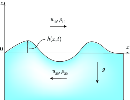
Figure 1: Kelvin-Helmholtz instability is the result of PT-symmetry breaking.

Since the equilibrium is homogeneous in the $x$-direction, different Fourier components in the $x$-direction are decoupled, and we can investigate each Fourier component separately. Assuming $(\delta u_{i},\delta w_{i},\delta p_{i})\sim\exp(ikx)$ for a wavelength $k\in\mathbb{R},$ and linearizing the fluid system (10)-(13), we obtain

$$ik\delta u_{i}+\frac{\partial\delta w_{i}}{\partial z} =0\,,$$ (18)

$$\frac{\partial\delta u_{i}}{\partial t}+u_{i0}ik\delta u_{i} =-\frac{ik}{\rho_{i0}}\delta p_{i}\,,$$ (19)

$$\frac{\partial\delta w_{i}}{\partial t}+u_{i0}ik\delta w_{i} =-\frac{1}{\rho_{i0}}\frac{\partial\delta p_{i}}{\partial z}\,.$$ (20)

In Eqs. (18)-(20), $(\delta u_{i},\delta w_{i},\delta p_{i})$ represent the complex Fourier components of the perturbed fields at the wavelength $k$ in the $x$-direction. To simplify the notation, we have overloaded the symbols $(\delta u_{i},\delta w_{i},\delta p_{i})$ to represent both the real perturbed fields on $(x,z)$, as well as their complex amplitudes on the spectrum space. Simple manipulation of Eqs. (18)-(20) shows that

$$\frac{\partial^{2}}{\partial z^{2}}\left(\frac{\partial\delta w_{1}}{\partial t}+iku_{10}\delta w_{1}\right)=\frac{\partial^{2}}{\partial z^{2}}\left(\frac{\partial\delta w_{2}}{\partial t}+iku_{20}\delta w_{2}\right)\,,$$

which implies that

$$(\delta w_{1},\delta p_{1}) \sim\exp(ikx-\left|k\right|z)\,,$$ (21)

$$(\delta w_{2},\delta p_{2}) \sim\exp(ikx+\left|k\right|z)\,,$$ (22)

where the boundary condition $\lim_{z\rightarrow\infty}\delta w_{1}=\lim_{z\rightarrow-\infty}\delta w_{2}=0$ has been incorporated. Note that the wavelength $k$ is allowed to be negative. With the $x$- and $z$-dependency specified by Eqs. (21) and (22), Eqs. (18)-(20) for the two layers of fluid $(i=1,2)$ reduce to, respectively,

$$ik\delta u_{1}-\left|k\right|\delta w_{1} =0\,,$$ (23)

$$\frac{\partial\delta u_{1}}{\partial t}+iku_{10}\delta u_{1} =-\frac{ik}{\rho_{10}}\delta p_{1}\,,$$ (24)

$$\frac{\partial\delta w_{1}}{\partial t}+iku_{10}\delta w_{1} =\frac{\left|k\right|}{\rho_{10}}\delta p_{1}\,,$$ (25)

and

$$ik\delta u_{2}+\left|k\right|\delta w_{2} =0\,,$$ (26)

$$\frac{\partial\delta u_{2}}{\partial t}+iku_{20}\delta u_{2} =-\frac{ik}{\rho_{20}}\delta p_{2}\,,$$ (27)

$$\frac{\partial\delta w_{2}}{\partial t}+iku_{20}\delta w_{2} =-\frac{\left|k\right|}{\rho_{20}}\delta p_{2}\,.$$ (28)

Now we invoke the boundary conditions at the interface,

$$\frac{d}{dt}\left(h(x,t)-z\right) =u_{i0}\frac{\partial h}{\partial x}+\frac{\partial h}{\partial t}-\frac{dz}{dt}=0,\,\,(i=1,2)\,,$$ (29)

$$p_{1}\mid_{z=h} =p_{2}\mid_{z=h}\,,$$ (30)

which, in terms of the perturbed fields, are

$$u_{i0}ikh+\frac{\partial h}{\partial t}-\delta w_{i} =0\,,\,\,(i=1,2)\,,$$ (31)

$$-\rho_{10}g+\delta p_{1} =-\rho_{20}g+\delta p_{2}\,,$$ (32)

Define $\phi_{1}\equiv-\delta w_{1}/\left|k\right|$ and $\phi_{2}\equiv\delta w_{2}/\left|k\right|$. Equations (23)-(28), (31) and (32) can be combined to give the governing ODEs for $\phi_{1}$, $\phi_{2},$ and $h,$

$$\phi_{1} =-\frac{1}{\left|k\right|}\left(\frac{\partial}{\partial t}+iku_{10}\right)h\,,$$ (33)

$$\phi{}_{2} =\frac{1}{\left|k\right|}\left(\frac{\partial}{\partial t}+iku_{20}\right)h\,,$$ (34)

$$\rho_{10}\left(\frac{\partial\phi_{1}}{\partial t}+iku_{10}\phi_{1}+gh\right) =-\rho_{20}\left(\frac{\partial\phi_{2}}{\partial t}+iku_{20}\phi_{2}+gh\right)\,.$$ (35)

Assuming $(\phi_{1},\phi_{2},h)\sim\exp(-i\omega t)$, we obtain from Eqs. (33)-(35) the dispersion relation of the dynamics,

$$\omega_{\pm}=k\frac{\rho_{10}u_{10}+\rho_{20}u_{20}}{\rho_{10}+\rho_{20}}\pm\sqrt{\left|k\right|g\frac{\rho_{20}-\rho_{10}}{\rho_{20}+\rho_{10}}-\frac{k^{2}\rho_{10}\rho_{20}(u_{10}-u_{20})^{2}}{(\rho_{10}+\rho_{20})^{2}}}\,.$$ (36)

For a given $k\in\mathbb{R},$ when $g(\rho_{20}^{2}-\rho_{10}^{2})>\left|k\right|\rho_{10}\rho_{20}(u_{10}-u_{20})^{2}$, the eigen-frequencies $\omega_{\pm}$ of the two-fluid interaction are real and the dynamics is stable. When $g(\rho_{20}^{2}-\rho_{10}^{2})<\left|k\right|\rho_{10}\rho_{20}(u_{10}-u_{20})^{2}$, the eigen-frequencies $\omega_{\pm}$ are a pair of complex conjugate numbers and the dynamics is unstable. This is the well-known KH instability. Since the gravity is considered, it includes the Rayleigh-Taylor instability as a special case. For this reason, it can also be called Kelvin-Helmholtz-Rayleigh-Taylor instability. The boundary between stability and instability is at $g(\rho_{20}^{2}-\rho_{10}^{2})=\left|k\right|\rho_{10}\rho_{20}(u_{10}-u_{20})^{2}$. Obviously, these spectrum properties of the KH instability are exactly the Properties (I) and (II) for a PT-symmetric system. This observation naturally begs the question: is the system governing the KH instability PT-symmetric?

The answer is affirmative. This discovery reveals, according to Property (III), that the classical KH instability is the result of PT-symmetry breaking. Now we prove these facts explicitly and explain the interesting physics underpinning the mathematics.

Let’s start from the governing ODEs (33)-(35), which do not assume the form Eq. (1), the standard form for dynamic systems. A few lines of algebra show that Eqs. (33)-(35) actually describe a system with two independent complex variables. Therefore, we use Eq. (34) to eliminate $\phi_{2}$ in favor of $\phi_{1}$ and $h,$ and obtain

$$\left(\begin{array}[]{c}\dot{\phi}_{1}\\ \dot{h}\end{array}\right) =A\left(\begin{array}[]{c}\phi_{1}\\ h\end{array}\right)\,,$$ (41)

$$A =\left(\begin{array}[]{cc}\dfrac{ik\left(-u_{10}\rho_{10}-2u_{20}\rho_{20}+u_{10}\rho_{20}\right)}{\rho_{10}+\rho_{20}}&\dfrac{-\left|k\right|(u_{10}-u_{20})^{2}\rho_{20}+g(\rho_{20}-\rho_{10})}{\rho_{10}+\rho_{20}}\\ -\left|k\right|&-iku_{10}\end{array}\right)\,.$$ (44)

It can be verified that Eq. (41) is invariant under the following PT-transformation,

$$\left(\phi_{1},h,t,i\right)\rightarrow\left(-\phi_{1},h,-t,-i\right)\,.$$ (45)

In terms of matrix $A,$ this PT-symmetry is $PA+\bar{A}P=0$, i.e., Eq. (3), for

$$P=\left(\begin{array}[]{cc}-1&0\\ 0&1\end{array}\right)\,.$$ (46)

We have thus proved that governing equations of the KH instability is indeed PT-symmetric. This explains the spectrum Properties (I) and (II) of the system, and more importantly, stipulates that the KH instability occurs when and only when the PT-symmetry is broken.

To explicitly verify the PT-symmetry breaking as the mechanism for instability, we look at the eigenvectors $v_{\pm}$ of $H=iA,$

$$v_{\pm}= \left(\begin{array}[]{c}\pm i\bar{\phi}\\ 1\end{array}\right)\,,$$ (49)

$$\bar{\phi}= \frac{k(u_{20}-u_{10})\rho_{20}}{\left|k\right|(\rho_{10}+\rho_{20})}+\frac{1}{\left|k\right|}\sqrt{\left|k\right|g\frac{\rho_{20}-\rho_{10}}{\rho_{20}+\rho_{10}}-\frac{k^{2}\rho_{10}\rho_{20}(u_{10}-u_{20})^{2}}{(\rho_{10}+\rho_{20})^{2}}}\,.$$ (50)

When the system is stable, i.e., $g(\rho_{20}^{2}-\rho_{10}^{2})>\left|k\right|\rho_{10}\rho_{20}(u_{10}-u_{20})^{2}$, both eigenvectors $v_{\pm}$ preserve the PT-symmetry, which means that they are invariant under the PT-transformation (45). When the KH instability occurs, both eigenvectors are not invariant under the PT-transformation (45), and the PT-symmetry is broken. As a matter of fact, the PT-transformation (45) maps $v_{+}$ into $v_{-}$, and vice versa.

In terms of physics, the PT-symmetry of Eq. (41) can be traced all the way back to the fluid equations (10)-(13). We observe that the system is symmetric with respect to the following PT-transformation,

$$(t,u,w,p,\rho)\rightarrow(-t,-u,-w,p,\rho)\,.$$ (51)

This PT-symmetry is a discrete symmetry originates from the reversibility of the fluid system, which is expected for conservative classical systems governed by Newton’s second law in fluid dynamics and plasma physics. When the solutions of the system preserve this PT-symmetry, i.e., the PT-symmetry is unbroken, the dynamics is stable. On the other hand, when a solution is not invariant under the PT-transformation (51), the PT-symmetry is (spontaneously) broken and the system is unstable. This is the mechanism of the KH instability. Apparently, this instability mechanism applies to all instabilities that can be described by the fluid equations (10)-(13). The KH instability is just the one of them, admittedly the most famous one.

It should be evident that parity transformation will have a different form for different choices of dynamic variables. For example, we can define a pair of new variables as

$$\left(\begin{array}[]{c}\psi_{1}\\ \psi_{2}\end{array}\right)=Q\left(\begin{array}[]{c}\phi_{1}\\ h\end{array}\right)\,,\,\,\,Q\equiv\left(\begin{array}[]{cc}-1&u_{10}\\ 1&u_{10}\end{array}\right)\,.$$ (52)

In terms of $\psi_{1}$ and $\psi_{2}$, Eq. (41) is

$$\left(\begin{array}[]{c}\dot{\psi}_{1}\\ \dot{\psi}_{2}\end{array}\right)=QAQ^{-1}\left(\begin{array}[]{c}\psi_{1}\\ \psi_{2}\end{array}\right)\,.$$ (53)

Equation (53) is symmetric with respect to the following PT-transformation

$$\left(\psi_{1},\psi_{2},t,i\right)\rightarrow\left(\psi_{2},\psi_{1},-t,-i\right)\,,$$

which is probably more familiar than the one given by Eq. (45). But the difference is merely cosmetic.

Let’s finish our discussion with a few footnotes. First, we expect that all classical conservative systems governed by Newton’s law are PT-symmetric, since the PT-symmetry is a manifestation of the classical reversibility. As a consequence, we further expected all classical instabilities of conservative systems are the result of spontaneous PT-symmetry breaking. Secondly, the PT-symmetry can also be broken explicitly by the governing equations, as oppose to spontaneously by the solutions. This happens, for instance, when the system is dissipative due to mechanical frictions or radiation reaction force on charged particles. Interestingly, explicit PT-symmetry breaking due to dissipation can also lead to instabilities. Finally, specific classical systems may admit special PT-symmetries not necessarily associated with classical reversibility of conservative systems. For example, in stellarators, a family of non-axisymmetric magnetic confinement devices, PT-symmetry has been identified by Dewar and collaborators and its effects have been studied (Dewar and Meiss, 1992; Dewar and Hudson, 1998) .

Relevant results in these aspects will be reported in other publications.