Energy minimisers of prescribed winding number in an $\mathbb{S}^{1}$-valued nonlocal Allen-Cahn type model

Abstract

We study a variational model for transition layers in thin ferromagnetic films with an underlying functional that combines an Allen-Cahn type structure with an additional nonlocal interaction term. The model represents the magnetisation by a map from $\mathbb{R}$ to $\mathbb{S}^{1}$. Thus it has a topological invariant in the form of a winding number, and we study minimisers subject to a prescribed winding number. As shown in our previous paper [15], the nonlocal term gives rise to solutions that would not be present for a functional including only the (local) Allen-Cahn terms. We complete the picture here by proving existence of minimisers in all cases where it has been conjectured. In addition, we prove non-existence in some other cases.

Keywords: domain walls, Allen-Cahn, nonlocal, existence of minimizers, topological degree, concentration-compactness, micromagnetics.

1 Introduction

In this paper we study a variational model coming from the theory of micromagnetics. In soft thin films of ferromagnetic materials, one of the predominant structures in the magnetisation field is a type of transition layer, called a Néel wall. We consider a simplified, one-dimensional variational model for Néel walls and study the question whether several transitions may combine to form a more complex transition layer. The same model has been used by several authors to analyse Néel walls in terms of existence, uniqueness, and properties of solutions to the Euler-Lagrange equations, but mostly for single transitions (see Section 1.2 for more details). For the background and the derivation of the model, we refer to the papers [6, 8, 11].

1.1 The model

We begin with a description of the variational model used for our theory. For a given parameter $h\in[0,1]$, consider maps $m=(m_{1},m_{2}):\mathbb{R}\to\mathbb{S}^{1}$ with values on the unit circle $\mathbb{S}^{1}$. We study the functional

$$E_{h}(m)=\frac{1}{2}\left(\|m^{\prime}\|^{2}_{L^{2}(\mathbb{R})}+\|m_{1}-h\|^{2}_{\dot{H}^{1/2}(\mathbb{R})}+\|m_{1}-h\|^{2}_{L^{2}(\mathbb{R})}\right),$$

where $m^{\prime}$ is the derivative of $m$ and $\dot{H}^{1/2}(\mathbb{R})$ denotes the homogeneous Sobolev space of order $1/2$ (a different representation of the corresponding term is given shortly). The first two terms in this functional represent what is called the exchange energy and the stray field energy in the full micromagnetic model, and we will use these expressions here as well. The third term comes from a combination of crystalline anisotropy and an external magnetic field. For simplicity, we call this term the anisotropy energy.

The stray field energy $\|m_{1}-h\|^{2}_{\dot{H}^{1/2}(\mathbb{R})}$ arises from the micromagnetic theory in conjunction with a stray field potential $u\colon\mathbb{R}_{+}^{2}\to\mathbb{R}$ (where $\mathbb{R}_{+}^{2}=\mathbb{R}\times(0,\infty)$), which solves

$$\Delta u =0 \text{in $\mathbb{R}_{+}^{2}$},$$ (1)

$$\frac{\partial u}{\partial x_{2}} =-m_{1}^{\prime} \text{on $\mathbb{R}\times\{0\}$}.$$ (2)

This boundary value problem has a unique solution up to constants if we impose finite Dirichlet energy. (We will discuss this point in more detail in Section 2.) The solution then satisfies

$$\int_{\mathbb{R}_{+}^{2}}|\nabla u|^{2}\,dx=\|m_{1}-h\|^{2}_{\dot{H}^{1/2}(\mathbb{R})}.$$

(The constant $h$ may seem irrelevant here, because $\|{\mkern 2.0mu\cdot\mkern 2.0mu}\|_{\dot{H}^{1/2}(\mathbb{R})}$ is a seminorm that vanishes on constant functions. Notwithstanding, we will keep $h$ in the expression as a reminder that $m_{1}-h$ decays to $0$ at $\pm\infty$ for the profiles we are interested in.) For some of the arguments in this paper, however, the following double integral representation is more convenient (see, e.g., [9]):

$$\|m_{1}-h\|^{2}_{\dot{H}^{1/2}(\mathbb{R})}=\frac{1}{2\pi}\int_{\mathbb{R}}\int_{\mathbb{R}}\frac{|m_{1}(x_{1})-m_{1}(y_{1})|^{2}}{|x_{1}-y_{1}|^{2}}\,dx_{1}dy_{1}.$$ (3)

As remarked previously, the third term in the energy functional represents, up to the constant $h^{2}$, the combined effects of the anisotropy potential $V(m)=m_{1}^{2}=1-m_{2}^{2}$ (favouring the easy axis $\pm e_{2}$) and the external field $-2he_{1}$ (favouring the direction $e_{1}=(1,0)$ for positive $h$) that gives rise to the term $-2he_{1}\cdot m=-2hm_{1}$. We denote

$$\alpha=\arccos h\in[0,\pi/2],$$

and we assume this relationship between $h$ and $\alpha$ throughout the paper. Then the resulting potential

$$W(m)=(m_{1}-h)^{2},\quad m\in\mathbb{S}^{1},$$

has two wells on the unit circle if $h\in[0,1)$, which are at $(\cos\alpha,\pm\sin\alpha)$, and one well at $(1,0)$ if $h=1$. If we write $m=(\cos\phi,\sin\phi)\in\mathbb{S}^{1}$, then we can further observe that $W$ grows quadratically in $\phi\pm\alpha$ near these wells if $h<1$ and quartically in $\phi$ near the well $(1,0)$ if $h=1$.

In principle, we could allow $h>1$ as well, but the questions studied in this paper are completely understood in this case by our previous work [15]. Since the case $h>1$ would require a somewhat different representation of the potential $W$, we omit the discussion here; however, we wish to point out that our previous paper [15] also partially treats the case $h\in[0,1)$ (in addition to $h>1$), but not $h=1$, because the quartic growth of $W$ near the wells is not compatible with the methods used there. From the physical point of view, the cases $h\geq 1$ and $h<1$ are equally interesting, but mathematically the latter is more interesting because it gives rise to the more intricate patterns.

1.2 Néel walls

A transition of $m$ between the wells of the potential $W$ on $\mathbb{S}^{1}$, as illustrated in Figure 1, represents a Néel wall (in the micromagnetics terminology). In the case of $h=1$ a transition means that $m$ describes a full rotation around $\mathbb{S}^{1}$. Thus in this case, we have the transition angles $\pm 2\pi$, while for $1>h=\cos\alpha$, we have the possible transitions angles $\pm 2\alpha$ and $\pm 2(\pi-\alpha)$ (see Figure 1).

Figure 1: Schematic representation of a Néel wall of angle $2\alpha$ (left) and $2\pi-2\alpha$ (right).

These are the most simple transitions, going from one well to the next. It is also conceivable, however, that $m$ will pass several wells during the transition. Such behaviour is in fact necessary for profiles of winding number $1$ or above (in the case $h<1$), which is why we discuss the winding number in the next section.

Existence, uniqueness and structure of locally energy minimising profiles including a Néel wall of angle $2\alpha$, for $\alpha\in(0,\frac{\pi}{2}]$, have been proved in [10, 15, 21, 22]. In this context, a Néel wall of angle $2\alpha$ is a (unique) two-scale object: it has a core of length $l\sim 1$ and two tails of larger length scale $\gg l$, where $m_{1}-h$ decays logarithmically. Stability, compactness, and optimality of Néel walls under two-dimensional perturbations have been proved in [2, 5, 16]. Existence and uniqueness results are also available for Néel walls of larger angle $\alpha\in(\frac{\pi}{2},\pi)$ (see [1, 15]) as well as for transition layers with prescribed winding number combining several Néel walls (see [12, 15]). Furthermore, the interaction between several Néel walls has been determined in terms of the energy (see [7, 14]).

1.3 Winding number

To each finite energy configuration $m:\mathbb{R}\to\mathbb{S}^{1}$ we associate a winding number $\deg(m)$ as follows. We first note that a map $m\in H_{\mathrm{loc}}^{1}(\mathbb{R};\mathbb{S}^{1})$ is necessarily continuous and has a continuous lifting $\phi\colon\mathbb{R}\to\mathbb{R}$ with $m=(\cos\phi,\sin\phi)$ in $\mathbb{R}$. Moreover, the lifting $\phi$ is unique up to a constant. If $E_{h}(m)<\infty$, then it follows that $\lim_{x_{1}\to\pm\infty}m(x_{1})=(\cos\alpha,\pm\sin\alpha)$ (where the signs on both sides of the equation are independent of one another). Thus

$$\deg(m)=\frac{1}{2\pi}\lim_{x_{1}\to\infty}(\phi(x_{1})-\phi(-x_{1}))$$

is well-defined and belongs to $\mathbb{Z}\pm\{0,\alpha/\pi\}$.

1.4 Objective of the paper

Our aim is to analyse the existence of minimisers $m$ of $E_{h}$ subject to a prescribed winding number. For $d\in\mathbb{Z}\pm\{0,\alpha/\pi\}$, we define

$$\mathcal{A}_{h}(d)=\left\{m\in H_{\mathrm{loc}}^{1}(\mathbb{R};\mathbb{S}^{1})\colon E_{h}(m)<\infty\text{ and }\deg(m)=d\right\}$$

and

$$\mathcal{E}_{h}(d)=\inf_{m\in\mathcal{A}_{h}(d)}E_{h}(m).$$

If we can find a minimiser of $E_{h}$ within $\mathcal{A}_{h}(d)$, then this will automatically be a critical point of winding number $d$. It will in general consist of several transitions between the points $(\cos\alpha,\pm\sin\alpha)$ on the unit circle; therefore, it can be thought of as a composite Néel wall consisting of several transitions stuck together. The first component $m_{1}$ of such configurations is shown schematically in Figures 2 and 3.

Figure 2: For $h=1$, an array of Néel walls of total winding number $3$, represented in terms of $m_{1}$.

Figure 3: For $h<1$, a hypothetical array of Néel walls of total winding number $1+\alpha/\pi$ (left) and an existing one of winding number $3-\alpha/\pi$ (right).

Clearly, there is a minimiser in $\mathcal{A}_{h}(0)$, which is constant. Moreover, it suffices to study the question for $d\geq 0$, as the case $d<0$ can be reduced to this one by reversing the orientation. It is well-known that a minimiser in $\mathcal{A}_{h}(\alpha/\pi)$ exists [21, 1], and similar arguments apply to $\mathcal{A}_{h}(1-\alpha/\pi)$ as well (see [15] for the details). We obtained further, but still partial results on the existence of minimisers in our previous paper [15]. Namely, there exist no minimisers in $\mathcal{A}_{h}(1)$, but if $\alpha>0$ is sufficiently small, then there exists a minimiser in $\mathcal{A}_{h}(2-\alpha/\pi)$. In this paper, we completely settle the question under the assumption that $\alpha$ is small enough (i.e., that $h$ is sufficiently close to $1$). We also have some information about the structure of the minimisers.

1.5 Main results

Our main results are as follows.

Theorem 1 (Existence of composite Néel walls).

Given $\ell\in\mathbb{N}=\{1,2,\dots\}$, there exists $H_{\ell}^{-}\in(0,1)$ such that $E_{h}$ attains its infimum in $\mathcal{A}_{h}(\ell-\alpha/\pi)$ for all $h\in(H_{\ell}^{-},1]$.

In the case $h=1$, we note that $\ell-\alpha/\pi=\ell$. Thus the following corollary is a special case of Theorem 1. We state it separately, because it highlights how the result fits in with a result for $h>1$ in our previous paper [15]. (The case $h=1$ was not studied in [15], so this is new information that complements the previous results.)

Corollary 2.

The functional $E_{1}$ attains its infimum in $\mathcal{A}_{1}(\ell)$ for every $\ell\in\mathbb{Z}$.

Theorem 3 (Non-existence).

Given $\ell\in\mathbb{N}$, there exist $H_{\ell}^{0},H_{\ell}^{+}\in(0,1)$ such that $E_{h}$ does not attain its infimum in $\mathcal{A}_{h}(\ell)$ for all $h\in(H_{\ell}^{0},1)$ and does not attain its infimum in $\mathcal{A}_{h}(\ell+\alpha/\pi)$ for all $h\in(H_{\ell}^{+},1)$.

The statements of Theorems 1 and 3 were conjectured in our previous paper [15], along with the conjecture that minimisers in $\mathcal{A}_{h}(\ell-\alpha/\pi)$ do not exist for $\ell\geq 2$ if $h$ is too small, and that the non-existence in $\mathcal{A}_{h}(\ell)$ and in $\mathcal{A}_{h}(\ell+\alpha/\pi)$ holds for all $h\in(0,1)$. Heuristic arguments were provided to back up the conjectures. They rely on a decomposition of $m_{1}-h$ into its positive and negative parts and a further decomposition into pieces that correspond to individual transitions between $(\cos\alpha,\pm\sin\alpha)$. The key observation is that the stray field energy (the nonlocal term in the functional) will become smaller if two pieces of the same sign approach each other or two pieces of opposite signs move away from each other. We may interpret this as attraction between pieces of the same sign and repulsion between pieces of opposite signs. If $1-h$ is small, then we also expect that the positive pieces will be much smaller than the negative pieces. Thus for winding number $\ell-\alpha/\pi$ for $\ell\in\mathbb{N}$ (as on the right of Figure 3), the whole profile will be sandwiched between the outermost pieces, which strongly attract each other. In contrast, for the winding number $\ell+\alpha/\pi$ (as on the left of Figure 3), the outermost pieces will experience a net repulsion, and moving these pieces towards $\pm\infty$ will reduce the energy.

We summarise our results and previously known results graphically in Figure 4, alongside some conjectures from our previous paper [15]. These conjectures would, if proved correct, complete the picture about the existence and non-existence of minimisers of $E_{h}$ subject to a prescribed winding number, except that the best values of $H_{\ell}^{-}$, $H_{\ell}^{0}$, and $H_{\ell}^{+}$ in Theorems 1 and 3 are still unknown. (Figure 4 might suggest that they are increasing in $\ell$, but no such statement is intended and their behaviour is unknown.)

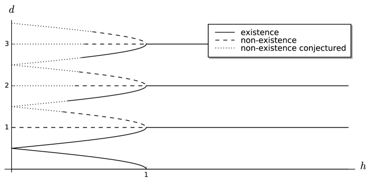
Figure 4: A schematic representation of existence and non-existence results and further conjectures. The position of any changeover between solid/dashed and dotted lines is not accurate.

For the proofs of Theorems 1 and 3, we need to quantify the above heuristic arguments precisely. Moreover, we need to estimate any effects coming from the other (local) terms in the energy functional as well, so that we can show that the above effects (coming from the nonlocal term) really do dominate the behaviour. In our previous paper [15], we used a linearisation of the Euler-Lagrange equation for minimisers of $E_{h}$ as one of our principal tools. This approach is based on ideas of Chermisi-Muratov [1]. It has the disadvantage, however, that it requires the quadratic growth of $W$ near the wells that we have observed for $h<1$ but not for $h=1$. There are further complications of a technical nature, and as a result, the method gives good estimates (in the case $h<1$) near the tails of a profile, but not between two Néel walls. This in turn restricts the analysis to small winding numbers. In this paper, we replace this tool with different arguments of variational nature. Our new estimates are more robust; in particular they do not have the restrictions described.

In the next step, we use the estimates to show that for certain profiles of $m$, splitting them into several parts of lower winding number will always increase the energy. In the concentration-compactness framework of Lions [20], this implies that no dichotomy will occur for minimising sequences. Here the strategy for the proof of Theorem 1 is similar to our previous paper [15]. For the non-existence, we have exactly the opposite: profiles of certain winding numbers can always be split into several parts in a way that decreases the energy.

In a forthcoming paper [13] (extending previous work [14]), we also study the asymptotic behaviour of a version of the problem where the exchange energy is weighted with a parameter $\epsilon$ that tends to $0$. The above heuristics are consistent with the observation that in this situation, too, the Néel walls stay away from each other when $\alpha\in(0,\frac{\pi}{2}]$ is sufficiently large. But for the asymptotic problem, we can give the precise angle where the change in behaviour occurs.

In addition to existence, we can give some information about the structure of the minimisers from Theorem 1.

Theorem 4 (Structure).

Given $\ell\in\mathbb{N}$, there exists $H_{\ell}\in(0,1)$ such that the following holds true for all $h\in(H_{\ell},1)$: if $m\in\mathcal{A}_{h}(\ell-\alpha/\pi)$ is a minimiser of $E_{h}$ in $\mathcal{A}_{h}(\ell-\alpha/\pi)$, then there exist $a_{1},\dotsc,a_{2\ell-1},b_{1},\dotsc,b_{2\ell-2}\in\mathbb{R}$ with

$$a_{1}<b_{1}<a_{2}<\dotsb<a_{2\ell-2}<b_{2\ell-2}<a_{2\ell-1}$$

such that $m_{1}(a_{n})=(-1)^{n}$ for $n=1,\dotsc,2\ell-1$ and $m_{1}\leq h$ in $(-\infty,b_{1}]\cup[b_{2},b_{3}]\cup\dotsb\cup[b_{2\ell-2},\infty)$ and $m_{1}\geq h$ in $[b_{1},b_{2}]\cup[b_{3},b_{4}]\cup\dotsb\cup[b_{2\ell-3},b_{2\ell-2}]$.

This means that the picture on the right of Figure 3 is qualitatively accurate. The result is also consistent with the idea that we should think of these minimisers as a composition of several Néel walls in a row.

It is an open question whether the minimisers of $E_{h}$ in $\mathcal{A}_{h}(\ell-\alpha/\pi)$ (in the cases where they exist) have a monotone phase. That is, if $m=(\cos\phi,\sin\phi)$ is such a minimiser, does it follow that $\phi^{\prime}\geq 0$ (or even $\phi^{\prime}>0$)? The answer is known only for the simplest cases of a transition of degree $\pm\alpha/\pi$ or $\pm(1-\alpha/\pi)$, where a standard symmetrisation argument applies (see [1, 21]). For a higher degree $\ell-\alpha/\pi$ with $\ell\geq 2$, Theorem 4 is consistent with a monotone phase, but it does of course not answer the question.

It is known, however, that the solutions of our minimisation problem are symmetric up to translation in the following sense [15, Lemma 3.2]: if $d\in\mathbb{N}-\alpha/\pi$ and $m\in\mathcal{A}_{h}(d)$ is a minimiser of $E_{h}$ in $\mathcal{A}_{h}(d)$, then there exists $t_{0}\in\mathbb{R}$ such that

$$m_{1}(t_{0}-x_{1})=m_{1}(t_{0}+x_{1})\quad\text{and}\quad m_{2}(t_{0}-x_{1})=-m_{2}(t_{0}+x_{1})$$

for all $x_{1}\in\mathbb{R}$.

Another open question is whether minimisers of $E_{h}$ in $\mathcal{A}_{h}(\ell-\alpha/\pi)$ are unique (up to translation in $x_{1}$) for $\ell\geq 2$. The answer is yes for $\mathcal{A}_{h}(\alpha/\pi)$ and for $\mathcal{A}_{h}(1-\alpha/\pi)$, as the energy is strictly convex in the $m_{1}$-component (see [14, Proposition 1]).

1.6 Scaling

The three terms in the energy $E_{h}(m)$ have different scaling. However, after rescaling in the variable $x_{1}$ and renormalizing the energy, only one length scale remains. This is why in the physical model, there is, in general, a parameter $\varepsilon$ in front of the exchange energy. As our results are qualitative (and not necessarily quantitative), we fix that parameter $\varepsilon=1$. The critical values $H_{\ell}$, $H_{\ell}^{0}$, $H_{\ell}^{+}$, and $H_{\ell}^{-}$ in our main results must of course be expected to depend on $\epsilon$. However, as we do not attempt to give the optimal values, we do not discuss this question any further.

For a critical point $m$ of the functional $E_{h}$, the Pohozaev identity (see [15, Proposition 1.1]) implies that we have equipartition of the energy coming from the local terms (the exchange and anisotropy energies). This equality effectively fixes the length scale of the core of a Néel wall (which is of order $l\sim 1$ for $\varepsilon=1$). The nonlocal term is dominant and has the length scale of the tails much larger than $l$.

1.7 Relation to other models

As we have mentioned in the introduction, the model studied in this paper can be seen as a nonlocal “perturbation” of the (local) Allen-Cahn model (the latter consisting only in the exchange and anisotropy terms), see [15, Appendix]. The nonlocal term in $E_{h}$ is in fact the key ingredient for existence of transition layers with higher winding number.

We can also relate our model to the study of $\frac{1}{2}$-harmonic maps defined on the real axis with values into the unit sphere (see, e.g., [4, 3] for regularity, compactness and bubble analysis and [23] for a Ginzburg-Landau approximation). There is a model for boundary vortices in micromagnetics (see e.g. [17, 18, 19, 24, 25]) that amounts to a “perturbation” of the $\frac{1}{2}$-harmonic map problem by a zero-order term comparable to the anisotropy in our model. But the problem studied in this paper has an additional higher-order term, which changes the behaviour of the problem dramatically. (This is most striking in the asymptotic analysis carried out in an earlier paper [14], where the interaction between different Néel walls is studied. We have attraction where the model for boundary vortices would give repulsion and vice versa.)

Acknowledgment.

R.I. acknowledges partial support by the ANR project ANR-14-CE25-0009-01.

2 Preliminaries

In this section we discuss a few tools for the analysis of our problem and recall some known results. Since the nonlocal term in the energy functional (i.e., the stray field energy) is not only the most challenging to analyse, but in fact determines the behaviour of the system to a considerable extent, it will have a prominent place here.

2.1 Representations of the stray field energy

We have already seen two different representations of the stray field energy. One of them is given by (3) and will be used in some of our estimates later on. The other representation involves the stray field potential $u$ that is determined by the boundary value problem (1), (2). In order to make the discussion of the problem rigorous, we introduce the inner product $\left\langle{\mkern 2.0mu\cdot\mkern 2.0mu},{\mkern 2.0mu\cdot\mkern 2.0mu}\right\rangle_{\dot{H}^{1}(\mathbb{R}_{+}^{2})}$ on the set of all $\phi\in C^{\infty}(\mathbb{R}\times[0,\infty))$ with compact support in $\mathbb{R}\times[0,\infty)$ (so $\phi$ is allowed to take non-zero values on the boundary $\mathbb{R}\times\{0\}$). This inner product is defined by the formula

$$\left\langle\phi,\psi\right\rangle_{\dot{H}^{1}(\mathbb{R}_{+}^{2})}=\int_{\mathbb{R}_{+}^{2}}\nabla\phi\cdot\nabla\psi\,dx.$$

The space $\dot{H}^{1}(\mathbb{R}_{+}^{2})$ is then the completion of the resulting inner product space. Its elements are not functions, strictly speaking, as the completion will conflate all constants. Nevertheless, we will sometimes implicitly pick a specific constant (for example, by considering the limit at $\infty$) and treat elements of $\dot{H}^{1}(\mathbb{R}_{+}^{2})$ as functions.

Given $m_{1}\in h+H^{1}(\mathbb{R})$, there exists a unique solution $u\in\dot{H}^{1}(\mathbb{R}_{+}^{2})$ of the boundary value problem (1), (2). This solution will satisfy

$$\|m_{1}-h\|_{\dot{H}^{1/2}(\mathbb{R})}^{2}=\int_{\mathbb{R}_{+}^{2}}|\nabla u|^{2}\,dx.$$

While it is sometimes convenient to work with $u$, there is also a dual problem that is more useful for other purposes. Namely, if $u\in\dot{H}^{1}(\mathbb{R}_{+}^{2})$ solves (1), (2), then we consider $\nabla^{\perp}u=(-\frac{\partial u}{\partial x_{2}},\frac{\partial u}{\partial x_{1}})$, which will satisfy $\operatorname{curl}\nabla^{\perp}u=0$ in $\mathbb{R}_{+}^{2}$. By the Poincaré lemma, there exists $v\colon\mathbb{R}_{+}^{2}\to\mathbb{R}$ such that $\nabla v=\nabla^{\perp}u$ (i.e., such that $u$ and $v$ are conjugate harmonic functions). This implies that $\Delta v=0$ in $\mathbb{R}_{+}^{2}$ and $\frac{\partial v}{\partial x_{1}}({\mkern 2.0mu\cdot\mkern 2.0mu},0)=m_{1}^{\prime}$ in $\mathbb{R}$. After adding a suitable constant, we thus obtain a solution of the boundary value problem

$$\Delta v =0 \text{in $\mathbb{R}_{+}^{2}$},$$ (4)

$$v =m_{1}-h \text{on $\mathbb{R}\times\{0\}$}.$$ (5)

If we are content to fix $v$ only up to a constant, then we may regard it as an element of $\dot{H}^{1}(\mathbb{R}_{+}^{2})$. Of course we also have the identity

$$\|m_{1}-h\|_{\dot{H}^{1/2}(\mathbb{R})}^{2}=\int_{\mathbb{R}_{+}^{2}}|\nabla v|^{2}\,dx,$$

which may be more familiar to the reader as $v$ is the harmonic extension of $m_{1}-h$ to the upper half-plane.

2.2 The Euler-Lagrange equation

As we are interested in minimising the functional $E_{h}$ in $\mathcal{A}_{h}(d)$, we will study the Euler-Lagrange equation for critical points of $E_{h}$. Given $m\colon\mathbb{R}\to\mathbb{S}^{1}$, it is convenient to represent the Euler-Lagrange equation in terms of the lifting $\phi\colon\mathbb{R}\to\mathbb{R}$. That is, we write $m=(\cos\phi,\sin\phi)$, and then the equation becomes

$$\phi^{\prime\prime}=(h-\cos\phi+u^{\prime}({\mkern 2.0mu\cdot\mkern 2.0mu},0))\sin\phi\quad\text{in $\mathbb{R}$}.$$ (6)

Here $u\in\dot{H}^{1}(\mathbb{R}_{+}^{2})$ is the stray field potential as introduced in the preceding section and we use the abbreviation $u^{\prime}=\frac{\partial u}{\partial x_{1}}$. The derivation of this equation is almost identical to the corresponding calculations given in our previous work [14]. It is known [15, Proposition 3.1] that solutions of (6) must be smooth.

If $m\in\mathcal{A}_{h}(d)$ for a given winding number $d$, then there will be at least a certain number of points, say $a_{1},\dotsc,a_{N}\in\mathbb{R}$, where $m_{1}(a_{n})=\pm 1$ and $m_{2}(a_{n})=0$ (i.e., $\phi(a_{n})\in\pi\mathbb{Z}$). We can use these points as a proxy for the positions of the Néel walls in the given configuration. One of the tasks for the proofs of the main theorems will be to estimate the rate of decay of $m_{1}-h$ as we move away from one of the points $a_{1},\dotsc,a_{N}$. But some information about these points is already available from our previous work [15, Lemma 3.1], namely that for energy minimising solutions of the Euler-Lagrange equation, the number $N$ is determined uniquely by the prescribed winding number. (Although it is assumed that $h\not=1$ in the other paper, the proof of this statement does not depend on the assumption.)

Lemma 5.

For any $h\in[0,1]$ and $d\in\mathbb{Z}\pm\{0,\alpha/\pi\}$, the following holds true.

1. Suppose that $d\not=0$ and $m\in\mathcal{A}_{h}(d)$ minimises $E_{h}$ in $\mathcal{A}_{h}(d)$. Then

   $$|m_{1}^{-1}(\{\pm 1\})|=\begin{cases}2|d|-1&\text{if $h=1$ and $d\in\mathbb{Z}$},\\ 2|d|&\text{if $h<1$ and $d\in\mathbb{Z}$},\\ 2\ell-1&\text{if $h<1$ and $|d|=\ell-1+\alpha/\pi$ or $|d|=\ell-\alpha/\pi$ with $\ell\in\mathbb{N}$}.\end{cases}$$

   Furthermore, if $a\in\mathbb{R}$ with $m_{1}(a)=\pm 1$, then $m_{2}^{\prime}(a)\not=0$. (Therefore, any lifting $\phi\colon\mathbb{R}\to\mathbb{R}$ of $m$ will satisfy $\phi^{\prime}(a)\neq 0$.)

2. If $0<|d|<1$, then $\mathcal{E}_{h}(d)\geq(1-\arccos(\pi d))^{2}$. If $|d|\geq 1$, then $\mathcal{E}_{h}(d)\geq 2|d|-1$. In particular, $\mathcal{E}_{h}(d)>0$ for every degree $d\neq 0$.

Proof.

Statement 1 was proved in [15, Lemma 3.1].

For statement 2, we observe the following. If $h\not=0$ and $m\in\mathcal{A}_{h}(\pm\alpha/\pi)$, then there exists $a\in\mathbb{R}$ such that $m_{1}(a)=1$, while $\lim_{x_{1}\to\pm\infty}m_{1}(x_{1})=h$. Thus

$$\int_{a}^{\infty}(|m^{\prime}|^{2}+(m_{1}-h)^{2})\,dx_{1}\geq 2\int_{a}^{\infty}|m_{1}^{\prime}||m_{1}-h|\,dx_{1}\geq(1-h)^{2}.$$

A similar estimate holds for the integral over $(-\infty,a)$. Hence $E_{h}(m)\geq(1-h)^{2}$.

If $h=0$ and $m\in\mathcal{A}_{h}(\pm 1/2)$, then we may have $a\in\mathbb{R}$ with $m_{1}(a)=-1$ instead, but this situation permits the same arguments.

If $m\in\mathcal{A}_{h}(d)$ for $d\not\in\{0,\pm\alpha/\pi\}$, then there exist at least $N\geq 2|d|-1$ points, say $a_{1},\dotsc,a_{N}\in\mathbb{R}$, with $a_{1}<\dotsb<a_{N}$ and $m_{1}(a_{n})=(-1)^{n}$ for $n=1,\dotsc,N$. Furthermore, there exist $b_{1},\dotsc,b_{N-1}\in\mathbb{R}$ such that $a_{n}<b_{n}\leq a_{n+1}$ and $m_{1}(b_{n})=h$ for $n=1,\dotsc,N-1$. Set $b_{0}=-\infty$ and $b_{N}=\infty$. Then by the same arguments as before,

$$\int_{a_{n}}^{b_{n}}(|m^{\prime}|^{2}+(m_{1}-h)^{2})\,dx_{1}\geq\left((-1)^{n}-h\right)^{2},\quad n=1,\dotsc,N.$$

Considering the intervals $(b_{n-1},a_{n})$ as well and summing over $n$, we then find that $E_{h}(m)\geq(1+h)^{2}$ if $d=\pm(1-\alpha/\pi)$ and $E_{h}(m)\geq 2|d|-1$ otherwise. ∎

Remark 6.

We recall that the following was proved in [15, Propositions 2.2 and 2.3].

1. (Monotonicity) If $d_{1},d_{2}\in\mathbb{Z}+\{0,\pm\alpha/\pi\}$ with $0\leq d_{1}\leq d_{2}$ (and if $0<h<1$, we suppose that $(d_{1},d_{2})\neq(\ell+\alpha/\pi,1+\ell-\alpha/\pi)$ for $\ell\in\mathbb{Z}$), then $\mathcal{E}_{h}(d_{1})\leq\mathcal{E}_{h}(d_{2})$. This is because a transition of degree $d_{2}$ contains also a (sub)transition of degree $d_{1}$, except for the exceptional case described above.

2. (Subadditivity) If $d_{1},d_{2},d\in\mathbb{Z}+\{0,\pm\alpha/\pi\}$ with $d_{1}+d_{2}=d$ (if $h=\cos\frac{\pi}{3}$ and $d_{2}-d_{1}\in\mathbb{Z}$, we suppose that $d\in\mathbb{Z}$), then $\mathcal{E}_{h}(d)\leq\mathcal{E}_{h}(d_{1})+\mathcal{E}_{h}(d_{2})$. This is because the concatenation of two transitions of degrees $d_{1}$ and $d_{2}$ has more energy than an optimal transition of degree $d_{1}+d_{2}$. Two such neighbouring transitions are compatible if either $d_{1}$ or $d_{2}$ is an integer, or if $d_{1}+d_{2}\in\mathbb{Z}$; this explains the constraint above for $h=\cos\frac{\pi}{3}$.

2.3 $H^{1}$ and $H^{2}$-estimates away from the Néel walls

The following is a consequence of the Euler-Lagrange equation, obtained by the use of suitable test functions and differentiation. It provides local estimates for a solution of (6) away from the points $a_{1},\dotsc,a_{N}$ where $m_{1}$ takes the value $\pm 1$ (thought of as the locations of the Néel walls and discussed in the preceding section).

The following inequalities include the energy density of the stray field energy, given in terms of the solution $v\in\dot{H}^{1}(\mathbb{R}_{+}^{2})$ of (4), (5). As a consequence, we have inequalities involving integrals over $\mathbb{R}$ and over $\mathbb{R}_{+}^{2}$ simultaneously. For convenience, we use the following shorthand notation: given a function $f\colon\mathbb{R}_{+}^{2}\to\mathbb{R}$, we write

$$\int_{-\infty}^{\infty}f\,dx_{1}=\int_{-\infty}^{\infty}f(x_{1},0)\,dx_{1}.$$

Proposition 7.

Let $h\in[0,1]$. Suppose that $I\subseteq\mathbb{R}$ is an open set and $\phi\in H_{\mathrm{loc}}^{1}(\mathbb{R})$. Let $m=(\cos\phi,\sin\phi)$ and suppose that $m_{1}-h\in\dot{H}^{1/2}(\mathbb{R})$ and $m_{2}(x_{1})\not=0$ for all $x_{1}\in I$. Let $\eta\in C_{0}^{\infty}(\mathbb{R}^{2})$ with $\operatorname{supp}\eta({\mkern 2.0mu\cdot\mkern 2.0mu},0)\subseteq I$. Suppose that $v\in\dot{H}^{1}(\mathbb{R}_{+}^{2})$ is the unique solution of $\Delta v=0$ in $\mathbb{R}_{+}^{2}$ with $v(x_{1},0)=m_{1}(x_{1})-h$ for all $x_{1}\in\mathbb{R}$. If $\phi$ is a solution of (6) in $I$, then

$$\int_{-\infty}^{\infty}\eta^{4}\left(\frac{1}{2}|m^{\prime}|^{2}+(m_{1}-h)^{2}\right)\,dx_{1}+\int_{\mathbb{R}_{+}^{2}}\eta^{4}|\nabla v|^{2}\,dx\\ \leq 576\int_{-\infty}^{\infty}(\eta^{\prime})^{4}\,dx_{1}+16\int_{\mathbb{R}_{+}^{2}}v^{2}\eta^{2}|\nabla\eta|^{2}\,dx$$ (7)

and

$$\int_{-\infty}^{\infty}\eta^{2}\left(|m^{\prime\prime}|^{2}+(m_{1}^{\prime})^{2}+\frac{|m^{\prime}|^{4}}{m_{2}^{2}}\right)\,dx_{1}+\int_{\mathbb{R}_{+}^{2}}\eta^{2}|\nabla^{2}v|^{2}\,dx\\ \leq 32\int_{-\infty}^{\infty}(\eta^{\prime})^{2}|m^{\prime}|^{2}\,dx_{1}+24\int_{\mathbb{R}_{+}^{2}}|\nabla\eta|^{2}|\nabla v|^{2}\,dx.$$ (8)

Proof.

If $u\in\dot{H}^{1}(\mathbb{R}_{+}^{2})$ is the solution of (1), (2), then $u$ and $v$ are conjugate harmonic functions in the sense that $\nabla v=\nabla^{\perp}u$. Thus equation (6) may be written in the form

$$\phi^{\prime\prime}=\left(h-\cos\phi+\frac{\partial v}{\partial x_{2}}\right)\sin\phi.$$

Since $\sin\phi\neq 0$ in $I$, then

$$v({\mkern 2.0mu\cdot\mkern 2.0mu},0)\frac{\partial v}{\partial x_{2}}({\mkern 2.0mu\cdot\mkern 2.0mu},0)=\phi^{\prime\prime}\frac{\cos\phi-h}{\sin\phi}+(\cos\phi-h)^{2}$$

in $I$. It follows that

$$\begin{split}\int_{\mathbb{R}_{+}^{2}}\eta^{4}|\nabla v|^{2}\,dx&=-\int_{-\infty}^{\infty}\eta^{4}v\frac{\partial v}{\partial x_{2}}\,dx_{1}-4\int_{\mathbb{R}_{+}^{2}}\eta^{3}v\nabla\eta\cdot\nabla v\,dx\\ &=-\int_{-\infty}^{\infty}\eta^{4}(\cos\phi-h)^{2}\,dx_{1}+\int_{-\infty}^{\infty}\eta^{4}(\phi^{\prime})^{2}\frac{h\cos\phi-1}{\sin^{2}\phi}\,dx_{1}\\ &\quad+4\int_{-\infty}^{\infty}\eta^{3}\eta^{\prime}\phi^{\prime}\frac{\cos\phi-h}{\sin\phi}\,dx_{1}-4\int_{\mathbb{R}_{+}^{2}}\eta^{3}v\nabla\eta\cdot\nabla v\,dx.\end{split}$$

We claim that

$$|\cos\phi-h|\leq 3(1-h\cos\phi).$$ (9)

For $0\leq h\leq\frac{1}{3}$, this is clear as $|\cos\phi-h|\leq 2$ and $1-h\cos\phi\geq\frac{2}{3}$ in this case. For $1\geq h>\frac{1}{3}$, we note that on the one hand,

$$h(\cos\phi-h)\leq 1-h\cos\phi,$$

because

$$2\cos\phi\leq 2\leq\frac{1}{h}+h,$$

and on the other hand,

$$h(h-\cos\phi)\leq 1-h\cos\phi$$

trivially. Hence (9) follows.

In particular, using Young’s inequality with three factors and exponents $2$, $4$, and $4$, we may estimate

$$\begin{split}4\int_{-\infty}^{\infty}\eta^{3}\eta^{\prime}\phi^{\prime}\frac{\cos\phi-h}{\sin\phi}\,dx_{1}&\leq\frac{1}{2}\int_{-\infty}^{\infty}\eta^{4}(\phi^{\prime})^{2}\frac{|\cos\phi-h|}{3\sin^{2}\phi}\,dx_{1}\\ &\quad+\frac{1}{2}\int_{-\infty}^{\infty}\eta^{4}(\cos\phi-h)^{2}\,dx_{1}+288\int_{-\infty}^{\infty}(\eta^{\prime})^{4}\,dx_{1}\\ &\stackrel{{\scriptstyle\eqref{eqn:inequality_for_cos_phi}}}{{\leq}}\frac{1}{2}\int_{-\infty}^{\infty}\eta^{4}(\phi^{\prime})^{2}\frac{1-h\cos\phi}{\sin^{2}\phi}\,dx_{1}\\ &\quad+\frac{1}{2}\int_{-\infty}^{\infty}\eta^{4}(\cos\phi-h)^{2}\,dx_{1}+288\int_{-\infty}^{\infty}(\eta^{\prime})^{4}\,dx_{1}.\end{split}$$

Furthermore,

$$-4\int_{\mathbb{R}_{+}^{2}}\eta^{3}v\nabla\eta\cdot\nabla v\,dx\leq\frac{1}{2}\int_{\mathbb{R}_{+}^{2}}\eta^{4}|\nabla v|^{2}\,dx+8\int_{\mathbb{R}_{+}^{2}}v^{2}\eta^{2}|\nabla\eta|^{2}\,dx.$$

Hence

$$\frac{1}{2}\int_{-\infty}^{\infty}\eta^{4}\left((\phi^{\prime})^{2}\frac{1-h\cos\phi}{\sin^{2}\phi}+(\cos\phi-h)^{2}\right)\,dx_{1}+\frac{1}{2}\int_{\mathbb{R}_{+}^{2}}\eta^{4}|\nabla v|^{2}\,dx\\ \leq 288\int_{-\infty}^{\infty}(\eta^{\prime})^{4}\,dx_{1}+8\int_{\mathbb{R}_{+}^{2}}v^{2}\eta^{2}|\nabla\eta|^{2}\,dx.$$

By Lemma 24 in the appendix,

$$\frac{1-h\cos\phi}{\sin^{2}\phi}\geq\frac{1}{2}.$$

Thus, we obtain the first inequality.

The second inequality is a direct consequence of an estimate proved in our paper [15]. Let $u\in\dot{H}^{1}(\mathbb{R}_{+}^{2})$ be the solution of (1), (2). In the proof of [15, Lemma 3.3], it is shown that under the above assumptions,

$$\int_{-\infty}^{\infty}\eta^{2}\left((\phi^{\prime\prime})^{2}+2(\phi^{\prime})^{2}\sin^{2}\phi+\frac{1}{3}(\phi^{\prime})^{4}(1+\cot^{2}\phi)\right)\,dx_{1}+\frac{1}{2}\int_{\mathbb{R}_{+}^{2}}\eta^{2}|\nabla^{2}u|^{2}\,dx\\ \leq\frac{16}{3}\int_{-\infty}^{\infty}(\eta^{\prime})^{2}(\phi^{\prime})^{2}\,dx_{1}+4\int_{\mathbb{R}_{+}^{2}}|\nabla\eta|^{2}|\nabla u|^{2}\,dx.$$

Noting that $|\nabla u|=|\nabla v|$ and $|\nabla^{2}u|=|\nabla^{2}v|$, and that

$$|m^{\prime}|^{2}=(\phi^{\prime})^{2},\quad(m_{1}^{\prime})^{2}=(\phi^{\prime})^{2}\sin^{2}\phi,\quad\text{and}\quad|m^{\prime\prime}|^{2}=(\phi^{\prime\prime})^{2}+(\phi^{\prime})^{4},$$

we derive inequality (8). ∎

3 Decay estimates

We now study how fast $m_{1}-h$ decays when we move away from the points where $m_{1}$ takes one of the values $\pm 1$. For technical reasons, we proceed in two steps, first proving a preliminary estimate before improving it in the second step.

3.1 A preliminary $L^{\infty}$-estimate

Lemma 8.

There exists a constant $C>0$ such that the following inequality holds true. Suppose that $h\in[0,1]$ and $m\in H_{\mathrm{loc}}^{1}(\mathbb{R};\mathbb{S}^{1})$ is a critical point of $E_{h}$. For any $t\in\mathbb{R}$, let

$$\sigma(t)=1+\inf\left\{|t-x_{1}|\colon x_{1}\in\mathbb{R}\text{ with }m_{2}(x_{1})=0\right\}.$$

Then

$$|m_{1}(t)-h|\leq C(\sigma(t))^{-3/4}\sqrt{E_{h}(m)+1}$$

for all $t\in\mathbb{R}$.

Proof.

Let $v$ denote the solution of (4), (5).

As $|m_{1}-h|\leq 2$, it suffices to consider $t\in\mathbb{R}$ with $\sigma(t)\geq 4$. Let $R=\frac{\sigma(t)}{4}$ (so $R\geq 1$). Choosing a suitable cut-off function $\eta$ in (7) in Proposition 7, we see that

$$\int_{t-R}^{t+R}\left(|m^{\prime}|^{2}+(m_{1}-h)^{2}\right)\,dx_{1}\leq\frac{C_{1}\pi^{2}}{32R^{2}}\int_{\mathbb{R}\times(0,R)}v^{2}\,dx+\frac{C_{1}}{R^{3}}$$

for a universal constant $C_{1}$.

The boundary value problem (4), (5) gives rise to some estimates for $v$ with standard tools. In particular, according to Lemma 25 in the appendix (applied for $p=2$),

$$\begin{split}\int_{\mathbb{R}\times(0,R)}v^{2}\,dx\leq\frac{16R}{\pi^{2}}\int_{-\infty}^{\infty}(m_{1}-h)^{2}\,dx_{1}.\end{split}$$

This, combined with the above inequality, yields

$$\int_{t-R}^{t+R}\left(|m^{\prime}|^{2}+(m_{1}-h)^{2}\right)\,dx_{1}\leq\frac{C_{1}}{R}(E_{h}(m)+1).$$ (10)

Moreover, estimate (8) in Proposition 7 leads to

$$\int_{t-R}^{t+R}(m_{1}^{\prime})^{2}\,dx_{1}\leq\frac{C_{2}}{2R^{2}}E_{h}(m)$$

for a universal constant $C_{2}$. In particular, we deduce that

$$\left(\operatorname*{osc}_{[t-\sqrt{R},t+\sqrt{R}]}m_{1}\right)^{2}\leq\left(\int_{t-\sqrt{R}}^{t+\sqrt{R}}|m_{1}^{\prime}|\,dx_{1}\right)^{2}\leq\frac{C_{2}}{R^{3/2}}E_{h}(m).$$ (11)

Set

$$C_{0}=\sqrt{\frac{C_{1}}{2}}+\sqrt{C_{2}}.$$

We claim that

$$|m_{1}(t)-h|\leq\frac{C_{0}}{R^{3/4}}\sqrt{E_{h}(m)+1},$$

which will conclude the proof. Indeed, if we had the inequality

$$|m_{1}(t)-h|>\frac{C_{0}}{R^{3/4}}\sqrt{E_{h}(m)+1},$$

then it would follow from (11) that

$$|m_{1}(x_{1})-h|>\frac{C_{0}-\sqrt{C_{2}}}{R^{3/4}}\sqrt{E_{h}(m)+1}=\sqrt{\frac{C_{1}(E_{h}(m)+1)}{2R^{3/2}}}$$

for all $x_{1}\in[t-\sqrt{R},t+\sqrt{R}]$. Hence

$$\int_{t-\sqrt{R}}^{t+\sqrt{R}}(m_{1}-h)^{2}\,dx_{1}>\frac{C_{1}}{R}(E_{h}(m)+1),$$

which contradicts (10). ∎

3.2 A preliminary $L^{1}$-estimate

Eventually we want to estimate the $L^{1}$-norms of the positive and negative parts of $m_{1}-h$. The preceding inequality is not good enough for this purpose, but we will use it as a first step. In the next step (Lemma 9), we derive an $L^{2}$-estimate of $m_{1}-h$, before turning it into an $L^{1}$-estimate in Proposition 10 below.

Lemma 9.

Let $p\in(\frac{4}{3},2]$. Then there exists a number $C>0$ with the following property. Let $h\in[0,1]$ and $d\in\mathbb{Z}\pm\{0,\alpha/\pi\}$. Suppose that $m\in\mathcal{A}_{h}(d)$ is a minimiser of $E_{h}$ in $\mathcal{A}_{h}(d)$. Let $a_{1},a_{2}\in\mathbb{R}\cup\{\pm\infty\}$ with $a_{1}<a_{2}$ such that $m_{2}\not=0$ in $(a_{1},a_{2})$. Then

$$\int_{a_{1}+R}^{a_{2}-R}\left(|m^{\prime}|^{2}+(m_{1}-h)^{2}\right)\,dx_{1}\leq C(|d|+1)^{2/p}R^{-2/p}(E_{h}(m)+1)$$

for all $R\geq 1$.

Proof.

As in the proof of Proposition 7 and Lemma 8, let $v$ denote the harmonic extension of $m_{1}-h$ to $\mathbb{R}_{+}^{2}$. Then by Lemma 25 in the appendix, there exists a constant $C_{1}=C_{1}(p)$ such that

$$\int_{0}^{R}\int_{-\infty}^{\infty}v^{2}\,dx_{1}\,dx_{2}\leq C_{1}R^{2-2/p}\|m_{1}-h\|_{L^{p}(\mathbb{R})}^{2}.$$

Assuming that we have a cut-off function $\eta\in C_{0}^{\infty}(\mathbb{R}^{2})$ with $0\leq\eta\leq 1$ such that $\operatorname{supp}\eta\subseteq\mathbb{R}\times(-\infty,R]$ and $\operatorname{supp}\eta({\mkern 2.0mu\cdot\mkern 2.0mu},0)\subseteq(a_{1},a_{2})$, then (7) in Proposition 7 implies that

$$\int_{-\infty}^{\infty}\eta^{4}\left(\frac{1}{2}|m^{\prime}|^{2}+(m_{1}-h)^{2}\right)\,dx_{1}+\int_{\mathbb{R}_{+}^{2}}\eta^{4}|\nabla v|^{2}\,dx\\ \leq C_{2}R^{2-2/p}\|\nabla\eta\|_{L^{\infty}(\mathbb{R}_{+}^{2})}^{2}\|m_{1}-h\|_{L^{p}(\mathbb{R})}^{2}+576\|\eta^{\prime}\|_{L^{4}(\mathbb{R})}^{4},$$

where $C_{2}=16C_{1}$. A suitable choice of $\eta$ therefore gives rise to a number $C_{3}$, depending only on $p$, such that

$$\int_{a_{1}+R}^{a_{2}-R}\left(|m^{\prime}|^{2}+(m_{1}-h)^{2}\right)\,dx_{1}\leq C_{3}R^{-2/p}\|m_{1}-h\|_{L^{p}(\mathbb{R})}^{2}+C_{3}R^{-3}.$$

Furthermore, since $p>\frac{4}{3}$, the function $\sigma$ in Lemma 8 has the property that $\sigma^{-3p/4}$ is integrable over $\mathbb{R}$. Lemma 5 and Lemma 8 then imply that

$$\|m_{1}-h\|_{L^{p}(\mathbb{R})}\leq C_{4}(|d|+1)^{1/p}\sqrt{E_{h}(m)+1}$$

for some constant $C_{4}=C_{4}(p)$. Thus we obtain a constant $C_{5}=C_{5}(p)$ such that

$$\int_{a_{1}+R}^{a_{2}-R}\left(|m^{\prime}|^{2}+(m_{1}-h)^{2}\right)\,dx_{1}\leq C_{5}(|d|+1)^{2/p}R^{-2/p}(E_{h}(m)+1).$$

This is the desired estimate. ∎

The preceding result implies an $L^{1}$-estimate for the positive and negative parts of $m_{1}-h$. In the following, we write $(m_{1}-h)_{+}=\max\{m_{1}-h,0\}\geq 0$ and $(m_{1}-h)_{-}=\min\{m_{1}-h,0\}\leq 0$.

Proposition 10.

Let $p\in(\frac{4}{3},2)$. Then there exists a number $C>0$ with the following property. Let $h\in[0,1]$. Given $d\in\mathbb{Z}\pm\{0,\alpha/\pi\}$, suppose that $m\in\mathcal{A}_{h}(d)$ is a minimiser of $E_{h}$ in $\mathcal{A}_{h}(d)$. Then

$$\int_{-\infty}^{\infty}(m_{1}-h)_{+}\,dx_{1}\leq C(|d|+1)^{1+1/p}\alpha^{2(2-p)/(2+p)}\sqrt{E_{h}(m)+1}$$

and

$$-\int_{-\infty}^{\infty}(m_{1}-h)_{-}\,dx_{1}\leq C(|d|+1)^{1+1/p}\sqrt{E_{h}(m)+1}.$$

Proof.

Let $C_{1}$ be the constant satisfying the statement of Lemma 9 for the given value of $p$ and define

$$c_{0}=\frac{1}{\sqrt{C_{1}(|d|+1)^{2/p}(E_{h}(m)+1)}}.$$

By Lemma 5, there exist $a_{1},\dotsc,a_{N}\in\mathbb{R}$ with $a_{1}<\dotsb<a_{N}$ and $N\leq 2|d|+1$ such that $m_{2}(a_{n})=0$ for $n=1,\dotsc,N$ and $m_{2}\not=0$ in $\mathbb{R}\setminus\{a_{1},\dotsc,a_{N}\}$. Set $a_{0}=-\infty$ and $a_{N+1}=+\infty$. Fix $n\in\{1,\dotsc,N\}$.

Lemma 9 gives $L^{2}$-estimates for $m_{1}-h$ at first, but using it for varying values of $R$, we can derive an $L^{1}$-estimate as well. The details are given in Lemma 26 in the appendix. We apply this Lemma 26 to the functions

$$\psi_{1}(x_{1})=\begin{cases}c_{0}|m_{1}(a_{n}+x_{1})-h|&\text{if $1\leq x_{1}\leq(a_{n+1}-a_{n})/2$},\\ 0&\text{if $x_{1}>(a_{n+1}-a_{n})/2$},\end{cases}$$

and

$$\psi_{2}(x_{1})=\begin{cases}c_{0}|m_{1}(a_{n}-x_{1})-h|&\text{if $1\leq x_{1}\leq(a_{n}-a_{n-1})/2$},\\ 0&\text{if $x_{1}>(a_{n}-a_{n-1})/2$},\end{cases}$$

and use Lemma 9 to verify that the hypothesis of Lemma 26 is satisfied for $\sigma=2/p$. (This is why we assume $p<2$ here, in contrast to Lemma 9.) Therefore, there exists a constant $C_{2}=C_{2}(p)$ such that

$$\int_{(a_{n}+a_{n-1})/2}^{a_{n}-R}|m_{1}-h|\,dx_{1}\leq\frac{C_{2}R^{1/2-1/p}}{c_{0}}$$

and

$$\int_{a_{n}+R}^{(a_{n+1}+a_{n})/2}|m_{1}-h|\,dx_{1}\leq\frac{C_{2}R^{1/2-1/p}}{c_{0}}$$

for all $R\geq 1$.

If $\alpha\leq 1$, then we choose $R=\alpha^{-4p/(2+p)}$. Using the fact that $(m_{1}-h)_{+}\leq 1-h\leq\frac{\alpha^{2}}{2}$ in $(a_{n}-R,a_{n}+R)$, we then obtain the estimate

$$\int_{(a_{n}+a_{n-1})/2}^{(a_{n+1}+a_{n})/2}(m_{1}-h)_{+}\,dx_{1}\leq\left(\frac{2C_{2}}{c_{0}}+1\right)\alpha^{2(2-p)/(2+p)}.$$

Then it suffices to sum over $n=1,\dotsc,N$ to prove the first inequality.

For $\alpha>1$ and for the second inequality, we can use the same arguments with $R=1$, since $|m_{1}-h|\leq 2$ in $(a_{n}-R,a_{n}+R)$. ∎

3.3 Improved estimates

With this control of the $L^{1}$-norm, we can now take advantage of the second inequality in Lemma 25 and improve the estimates again.

Proposition 11.

There exists a number $C>0$ with the following property. Let $h\in[0,1]$ and suppose that $m\in\mathcal{A}_{h}(d)$ is a minimiser of $E_{h}$ in $\mathcal{A}_{h}(d)$ for some $d\in\mathbb{Z}\pm\{0,\alpha/\pi\}$. Let $u\in\dot{H}^{1}(\mathbb{R}_{+}^{2})$ denote the solution of (1), (2), and let $a_{1},a_{2}\in\mathbb{R}\cup\{\pm\infty\}$ with $a_{1}<a_{2}$ and $m_{2}\not=0$ in $(a_{1},a_{2})$. Then

$$\int_{a_{1}+R}^{a_{2}-R}\left(|m^{\prime}|^{2}+(m_{1}-h)^{2}\right)\,dx_{1}+\int_{a_{1}+R}^{a_{2}-R}\int_{0}^{R}|\nabla u|^{2}\,dx_{2}\,dx_{1}\\ \leq C(|d|+1)^{16/5}R^{-2}\log R\,(E_{h}(m)+1)$$ (12)

and

$$\int_{a_{1}+R}^{a_{2}-R}\left(|m^{\prime\prime}|^{2}+(m_{1}^{\prime})^{2}+\frac{|m^{\prime}|^{4}}{m_{2}^{2}}\right)\,dx_{1}+\int_{a_{1}+R}^{a_{2}-R}\int_{0}^{R}|\nabla^{2}u|^{2}\,dx_{2}\,dx_{1}\\ \leq C(|d|+1)^{16/5}R^{-4}\log R\,(E_{h}(m)+1)$$ (13)

and

$$\int_{a_{1}+R}^{a_{2}-R}(u^{\prime}(x_{1},0))^{2}\,dx_{1}\leq C(|d|+1)^{16/5}R^{-3}\log R\,(E_{h}(m)+1)$$ (14)

for all $R\geq 2$.

Proof.

For the proof of (12), we simply combine (7) in Proposition 7 with the second and third inequality of Lemma 25 and Proposition 10 (with $p=5/3$). Choosing a suitable cut-off function $\eta$ in Proposition 7, such that $\eta\equiv 1$ in $[a_{1}+R,a_{2}-R]\times[0,R]$,

$$\operatorname{supp}\nabla\eta\cap\mathbb{R}_{+}^{2}\subseteq\bigl{(}[a_{1}+R/2,a_{1}+R]\times(0,2R]\bigr{)}\cup{}\\ \cup\bigl{(}[a_{2}-R,a_{2}-R/2]\times(0,2R]\bigr{)}\cup\bigl{(}[a_{1}+R/2,a_{2}-R/2]\times[R,2R]\bigr{)},$$

and $|\nabla\eta|\leq 8/R$, we thus obtain (12).

In order to prove (13), we use (8) in Proposition 7 and choose $\eta$ similarly to the first part of this proof again. Then we use (12) (say, with $R/2$ instead of $R$) to estimate the right-hand side of (8). This gives the desired estimate.

Finally, for the proof of (14), we consider the conjugate harmonic function $v\colon\mathbb{R}_{+}^{2}\to\mathbb{R}$ with $\nabla v=\nabla^{\perp}u$. Again we choose $\eta\in C_{0}^{\infty}(\mathbb{R}^{2})$ and compute

$$\begin{split}\int_{-\infty}^{\infty}\eta^{2}(u^{\prime})^{2}\,dx_{1}&=\int_{-\infty}^{\infty}\eta^{2}\left(\frac{\partial v}{\partial x_{2}}(x_{1},0)\right)^{2}\,dx_{1}\\ &=-\int_{\mathbb{R}_{+}^{2}}\operatorname{div}\left(\eta^{2}\frac{\partial v}{\partial x_{2}}\nabla v\right)\,dx\\ &=-\int_{\mathbb{R}_{+}^{2}}\left(\eta^{2}\nabla v\cdot\nabla\frac{\partial v}{\partial x_{2}}+2\eta\frac{\partial v}{\partial x_{2}}\nabla\eta\cdot\nabla v\right)\,dx\\ &\leq\int_{\mathbb{R}_{+}^{2}}\bigg{(}\eta^{2}(R|\nabla^{2}v|^{2}+R^{-1}|\nabla v|^{2})+2|\eta||\nabla\eta||\nabla v|^{2}\bigg{)}\,dx.\end{split}$$

We observe that $|\nabla v|=|\nabla u|$ and $|\nabla^{2}v|=|\nabla^{2}u|$. Using (12) and (13) and choosing $\eta$ appropriately, we therefore obtain (14). ∎

4 Localisation

In the proofs of the main results, we need to estimate how the energy changes when we localise a given profile with a cut-off function. For $h<1$, we have suitable estimates from our previous work [15, Proposition 2.1]. For the case $h=1$, however, we need to modify the result.

Lemma 12.

There exists a constant $C>0$ with the following property. Suppose that $h=1$ and $\phi\in H_{\mathrm{loc}}^{1}(\mathbb{R})$ is such that $m=(\cos\phi,\sin\phi)$ satisfies $E_{1}(m)<\infty$. Let $v\in\dot{H}^{1}(\mathbb{R}_{+}^{2})$ be the solution of (4), (5). Furthermore, suppose that there exist two numbers $\ell_{\pm}\in 2\pi\mathbb{Z}$ and three measurable functions $\omega,\sigma,\tau\colon[0,\infty)\to[0,\infty)$ such that

$$|\phi(x_{1})-\ell_{+}|\leq\omega(x_{1})\quad\text{and}\quad|\phi(-x_{1})-\ell_{-}|\leq\omega(x_{1})\quad\text{for all $x_{1}\geq 0$}$$

and

$$|\phi^{\prime}(x_{1})|\leq\sigma(|x_{1}|)\quad\text{and}\quad\left|\frac{\partial v}{\partial x_{2}}(x_{1},0)\right|\leq\tau(|x_{1}|)\quad\text{for all $x_{1}\in\mathbb{R}$.}$$

Suppose that $\sup_{x_{1}\geq r}\omega(x_{1})\leq\frac{\pi}{2}$ for some $r\geq 1$. Then for any $R\geq r$ there exists $\tilde{m}\in H_{\mathrm{loc}}^{1}(\mathbb{R};\mathbb{S}^{1})$ such that

$$\deg(\tilde{m})=\frac{\ell_{+}-\ell_{-}}{2\pi}$$ (15)

and

$$\tilde{m}_{1}=1\text{ in $(-\infty,-2R]\cup[2R,\infty)$},\quad\tilde{m}_{1}=m_{1}\text{ in $[-R,R]$},$$

and $|\tilde{m}_{1}-1|\leq|m_{1}-1|$ everywhere, and such that

$$E_{1}(\tilde{m})\leq E_{1}(m)+\frac{C}{R^{2}}\int_{R}^{2R}\left(\omega^{2}+R\omega\sigma\right)\,dx_{1}+C\int_{R}^{\infty}\omega^{2}\tau\,dx_{1}\\ +C\left(\int_{R}^{\infty}\omega^{4}\,dx_{1}\right)^{1/2}\left(\int_{R}^{\infty}\left(\frac{\omega^{4}}{R^{2}}+\omega^{2}\sigma^{2}\right)\,dx_{1}\right)^{1/2}.$$

This result has a counterpart for $h\not=1$, stated in [15, Proposition 2.1]. For the purpose of this paper, however, only the case $h<1$ treated in [15] is relevant. The structure of the statement is then similar to the above lemma, but for $h<1$ the inequality becomes

$$E_{h}(\tilde{m})\leq E_{h}(m)+C\int_{R}^{\infty}\left(\frac{\omega^{2}}{R^{2}}+\sigma^{2}+\omega\tau\right)\,dx_{1}\\ +C\left(\int_{R}^{\infty}\omega^{2}\,dx_{1}\right)^{1/2}\left(\int_{R}^{\infty}\left(\frac{\omega^{2}}{R^{2}}+\sigma^{2}\right)\,dx_{1}\right)^{1/2}.$$ (16)

This is good enough for our proofs if $h<1$, but for $h=1$ we need the improvement given by Lemma 12.

The following proof is similar to the reasoning of [15, Proposition 2.1], too, but for the convenience of the reader, we repeat the arguments here.

Proof of Lemma 12.

Choose $\eta\in C_{0}^{\infty}(\mathbb{R})$ with $\eta(x_{1})=0$ for $|x_{1}|\geq 2R$ and $\eta(x_{1})=1$ for $|x_{1}|\leq R$, and such that $0\leq\eta\leq 1$ and $|\eta^{\prime}|\leq 2/R$ everywhere. Define

$$\tilde{\phi}(x_{1})=\begin{cases}\ell_{-}+\eta(x_{1})(\phi(x_{1})-\ell_{-})&\text{if $x_{1}\leq 0$},\\ \ell_{+}+\eta(x_{1})(\phi(x_{1})-\ell_{+})&\text{if $x_{1}>0$}.\end{cases}$$

Set $\tilde{m}=(\cos\tilde{\phi},\sin\tilde{\phi})$. Then clearly (15) is satisfied and $|\tilde{m}_{1}-1|\leq|m_{1}-1|$ everywhere.

For $x_{1}>0$, we compute

$$\tilde{\phi}^{\prime}(x_{1})=\eta(x_{1})\phi^{\prime}(x_{1})+\eta^{\prime}(x_{1})(\phi(x_{1})-\ell_{+}).$$

A similar identity holds for $x_{1}<0$. Hence

$$(\tilde{\phi}^{\prime})^{2}\leq(\phi^{\prime})^{2}+2|\eta\eta^{\prime}||\phi^{\prime}||\phi-\ell_{\pm}|+(\eta^{\prime})^{2}(\phi-\ell_{\pm})^{2}\leq(\phi^{\prime})^{2}+\bigg{(}\frac{4\omega^{2}}{R^{2}}+\frac{4\omega\sigma}{R}\bigg{)}{\bf 1}_{\{|x_{1}|\in[R,2R]\}}$$

(where for simplicity, we extend $\omega$ and $\sigma$ to $\mathbb{R}$ evenly). It follows that

$$\frac{1}{2}\int_{-\infty}^{\infty}(\tilde{\phi}^{\prime})^{2}\,dx_{1}\leq\frac{1}{2}\int_{-\infty}^{\infty}(\phi^{\prime})^{2}\,dx_{1}+\frac{4}{R^{2}}\int_{R}^{2R}\left(\omega^{2}+R\omega\sigma\right)\,dx_{1}.$$

It is obvious that

$$\frac{1}{2}\int_{-\infty}^{\infty}\left(\tilde{m}_{1}-1\right)^{2}\,dx_{1}\leq\frac{1}{2}\int_{-\infty}^{\infty}(m_{1}-1)^{2}\,dx_{1}.$$

This leaves the stray field energy to be estimated.

Note that

$$\left|\tilde{m}_{1}-m_{1}\right|\leq 1-m_{1}\leq(\phi-\ell_{\pm})^{2}\leq\omega^{2}$$

in $\mathbb{R}\setminus[-R,R]$, whereas

$$\begin{split}\left|\tilde{m}_{1}^{\prime}-m_{1}^{\prime}\right|&=|\big{(}\eta^{\prime}(\phi-\ell_{\pm})+\eta\phi^{\prime}\big{)}\sin\tilde{\phi}-\phi^{\prime}\sin\phi|\\ &\leq|\phi^{\prime}||\sin\phi-\eta\sin\tilde{\phi}|+|\eta^{\prime}||\phi-\ell_{\pm}||\sin\tilde{\phi}|\\ &\leq|\phi^{\prime}||\phi-\ell_{\pm}|+|\eta^{\prime}|(\phi-\ell_{\pm})^{2}\\ &\leq\omega\sigma+\frac{2\omega^{2}}{R}.\end{split}$$

Here we have used the inequality $|\sin\tilde{\phi}|=|\sin\big{(}\eta(\phi-\ell_{\pm})\big{)}|\leq|\eta||\phi-\ell_{\pm}|$ together with $|\sin t-\eta\sin(\eta t)|\leq|\sin t|\leq|t|$ for all $0\leq\eta\leq 1$ and $t\in[-\pi/2,\pi/2]$ (applied to $t:=\phi-\ell_{\pm}$). Thus by interpolation between $L^{2}(\mathbb{R})$ and $\dot{H}^{1}(\mathbb{R})$, we obtain

$$\left\|\tilde{m}_{1}-m_{1}\right\|_{\dot{H}^{1/2}(\mathbb{R})}^{2}\leq C_{1}\left(\int_{R}^{\infty}\omega^{4}\,dx_{1}\right)^{1/2}\left(\int_{R}^{\infty}\left(\frac{\omega^{4}}{R^{2}}+\omega^{2}\sigma^{2}\right)\,dx_{1}\right)^{1/2}$$

for some universal constant $C_{1}$.

Now recall that $v\in\dot{H}^{1}(\mathbb{R}_{+}^{2})$ is the harmonic extension of $m_{1}-1$ to $\mathbb{R}_{+}^{2}$ and let $\tilde{v}\in\dot{H}^{1}(\mathbb{R}_{+}^{2})$ be the harmonic extension of $\tilde{m}_{1}-1$. Then

$$\int_{\mathbb{R}_{+}^{2}}|\nabla\tilde{v}|^{2}\,dx=\int_{\mathbb{R}_{+}^{2}}|\nabla v|^{2}\,dx+\int_{\mathbb{R}_{+}^{2}}|\nabla v-\nabla\tilde{v}|^{2}\,dx-2\int_{\mathbb{R}_{+}^{2}}\nabla v\cdot(\nabla v-\nabla\tilde{v})\,dx.$$

We know that

$$\begin{split}\int_{\mathbb{R}_{+}^{2}}|\nabla v-\nabla\tilde{v}|^{2}\,dx&=\left\|m_{1}-\tilde{m}_{1}\right\|_{\dot{H}^{1/2}(\mathbb{R})}^{2}\\ &\leq C_{1}\left(\int_{R}^{\infty}\omega^{4}\,dx_{1}\right)^{1/2}\left(\int_{R}^{\infty}\left(\frac{\omega^{4}}{R^{2}}+\omega^{2}\sigma^{2}\right)\,dx_{1}\right)^{1/2}.\end{split}$$

Moreover, an integration by parts gives

$$-2\int_{\mathbb{R}_{+}^{2}}\nabla v\cdot(\nabla v-\nabla\tilde{v})\,dx=2\int_{-\infty}^{\infty}(m_{1}-\tilde{m}_{1})\frac{\partial v}{\partial x_{2}}\,dx_{1}\leq 4\int_{R}^{\infty}\omega^{2}\tau\,dx_{1}.$$

Hence

$$\frac{1}{2}\int_{\mathbb{R}_{+}^{2}}|\nabla\tilde{v}|^{2}\,dx\leq\frac{1}{2}\int_{\mathbb{R}_{+}^{2}}|\nabla v|^{2}\,dx\\ +\frac{C_{1}}{2}\left(\int_{R}^{\infty}\omega^{4}\,dx_{1}\right)^{1/2}\left(\int_{R}^{\infty}\left(\frac{\omega^{4}}{R^{2}}+\omega^{2}\sigma^{2}\right)\,dx_{1}\right)^{1/2}+2\int_{R}^{\infty}\omega^{2}\tau\,dx_{1}.$$

The desired inequality then follows. ∎

When we apply Lemma 12, we will consider a fixed $d\in\mathbb{Z}\pm\{0,\alpha/\pi\}$ and a profile $m$ that minimises $E_{h}$ in $\mathcal{A}_{h}(d)$. Then by Lemma 5, there exist $a_{1},\dotsc,a_{N}\in\mathbb{R}$ with $a_{1}<\dotsb<a_{N}$ and $N\leq 2|d|+1$ such that $m_{2}(a_{n})=0$ for $n=1,\dotsc,N$ and $m_{2}\not=0$ elsewhere. Thus Proposition 11 applies between any pair of points $(a_{n},a_{n+1})$ and also in $(-\infty,a_{1})$ and in $(a_{N},\infty)$. If $\phi$ is a lifting of $m$, choosing

$$\omega(x_{1}) =\max\{|\phi(x_{1})-\ell_{+}|,|\phi(-x_{1})-\ell_{-}|\}$$

$$\sigma(x_{1}) =\max\{|\phi^{\prime}(x_{1})|,|\phi^{\prime}(-x_{1})|\},$$ (17)

$$\tau(x_{1}) =\max\left\{\left|\frac{\partial v}{\partial x_{2}}(x_{1},0)\right|,\left|\frac{\partial v}{\partial x_{2}}(-x_{1},0)\right|\right\},$$

we then find, by Lemma 8, that $\omega(x_{1})\leq\frac{\pi}{2}$ for $|x_{1}|$ large enough. Moreover, we then obtain $(\phi(x_{1})-\ell_{\pm})^{2}\leq\pi(1-\cos\phi(x_{1}))=\pi(1-m_{1}(x_{1}))$ for $|x_{1}|$ large enough. We write $I=(-2R,-R)\cup(R,2R)$. Then Proposition 11 implies

$$\begin{split}\int_{R}^{2R}\omega^{2}\,dx_{1}&\leq\pi\int_{I}(1-m_{1})\,dx_{1}\\ &\leq\pi\left(2R\int_{I}(1-m_{1})^{2}\,dx_{1}\right)^{1/2}\leq C_{1}\sqrt{\frac{\log R}{R}}\end{split}$$ (18)

and

$$\begin{split}\int_{R}^{2R}\omega\sigma\,dx_{1}&\leq\sqrt{\pi}\int_{I}\sqrt{1-m_{1}}|m^{\prime}|\,dx_{1}\\ &\leq\sqrt{\pi}\left(2R\int_{I}(1-m_{1})^{2}\,dx_{1}\right)^{1/4}\left(\int_{I}|m^{\prime}|^{2}\,dx_{1}\right)^{1/2}\\ &\leq\frac{C_{1}}{R^{5/4}}(\log R)^{3/4}\end{split}$$ (19)

for a constant $C_{1}=C_{1}(d)$, provided that $R$ is sufficiently large. Moreover,

$$\int_{R}^{\infty}\omega^{4}\,dx_{1} \leq\pi^{2}\int_{\mathbb{R}\setminus(-R,R)}(m_{1}-1)^{2}\,dx_{1}\leq\frac{C_{1}}{R^{2}}\log R,$$ (20)

$$\int_{R}^{\infty}\omega^{2}\sigma^{2}\,dx_{1} \leq\pi\int_{\mathbb{R}\setminus(-R,R)}\left(\frac{(m_{1}-1)^{2}}{R}+R|m^{\prime}|^{4}\right)\,dx_{1}\leq\frac{C_{1}}{R^{3}}\log R,$$ (21)

$$\int_{R}^{\infty}\omega^{2}\tau\,dx_{1} \leq\pi\int_{\mathbb{R}\setminus(-R,R)}\left(R^{-1/2}(m_{1}-1)^{2}+R^{1/2}\left(\frac{\partial v}{\partial x_{2}}\right)^{2}\right)\,dx_{1}\leq\frac{C_{1}}{R^{5/2}}\log R.$$ (22)

In the case $h<1$, we use [15, Proposition 2.1] instead of Lemma 12, which gives rise to inequality (16). In this case, we know that $|\phi-\ell_{\pm}|\leq c|m_{1}-h|$ and $|\phi^{\prime}|\leq c|m_{1}^{\prime}|$, with a constant $c$ depending on $h$, when $|x_{1}|$ is sufficiently large. This gives rise to

$$\int_{R}^{\infty}\omega^{2}\,dx_{1} \leq c^{2}\int_{\mathbb{R}\setminus(-R,R)}(m_{1}-h)^{2}\,dx_{1}\leq\frac{C_{2}}{R^{2}}\log R,$$ (23)

$$\int_{R}^{\infty}\sigma^{2}\,dx_{1} \leq c^{2}\int_{\mathbb{R}\setminus(-R,R)}|m_{1}^{\prime}|^{2}\,dx_{1}\leq\frac{C_{2}}{R^{4}}\log R,$$ (24)

$$\int_{R}^{\infty}\omega\tau\,dx_{1} \leq c\int_{\mathbb{R}\setminus(-R,R)}\left(R^{-1/2}(m_{1}-h)^{2}+R^{1/2}(u^{\prime})^{2}\right)\,dx_{1}\leq\frac{C_{2}}{R^{5/2}}\log R$$ (25)

for a constant $C_{2}=C_{2}(d,h)$, provided that $R$ is sufficiently large. These estimates are not quite as good as the ones derived in [15], but they are sufficient for our purpose and they avoid a significant part of the previous analysis. This conclusion can be summarized as follows.

Corollary 13.

Let $h\in[0,1]$ and $d\in\mathbb{Z}\pm\{0,\alpha/\pi\}$. Suppose that $m$ is a minimizer of $\mathcal{E}_{h}(d)$ in $\mathcal{A}_{h}(d)$. Then there exist $R_{0}\geq 1$ and $\beta>0$ such that for every $R\geq R_{0}$, there exists $\tilde{m}\in\mathcal{A}_{h}(d)$ that is locally constant in $\mathbb{R}\setminus[-R,R]$ and satisfies

$$E_{h}(\tilde{m})\leq\mathcal{E}_{h}(d)+\frac{1}{R^{2+\beta}}$$

and $|\tilde{m}_{1}-h|\leq|m_{1}-h|$ everywhere in $\mathbb{R}$.

5 Proofs of the main results

5.1 Existence and non-existence of minimisers

For the proof Theorem 1, we can now largely use the arguments from our previous paper [15], but we replace the previous decay estimates by Proposition 11 and the previous $L^{1}$-estimates by Proposition 10. The main task is to estimate the stray field energy for potential minimisers of $E_{h}$. To this end, we divide $m_{1}-h$ into several pieces, each of which is either nonpositive or nonnegative in $\mathbb{R}$. As we may express the stray field energy in terms of the $\dot{H}^{1/2}$-inner product, the following estimate, given as Lemma 4.3 in [15], is particularly useful here.

Lemma 14.

Let $f,g\in\dot{H}^{1/2}(\mathbb{R})$ be nonnegative functions and suppose that there exists $R>0$ with $\operatorname{supp}f\subseteq[-2R,-R]$ and $\operatorname{supp}g\subseteq[R,2R]$. Then

$$-\frac{1}{4\pi R^{2}}\|f\|_{L^{1}(\mathbb{R})}\|g\|_{L^{1}(\mathbb{R})}\leq\left\langle f,g\right\rangle_{\dot{H}^{1/2}(\mathbb{R})}\leq-\frac{1}{16\pi R^{2}}\|f\|_{L^{1}(\mathbb{R})}\|g\|_{L^{1}(\mathbb{R})}.$$

Using this and the above estimates, we can now examine what happens if a magnetisation profile $m$ is split into two or more parts or if several profiles are combined. For this purpose, we use the following notion.

Definition 15.

Fix $h\in(0,1]$ and let $D_{h}=(\mathbb{N}\pm\{0,\alpha/\pi\})\cup\{\alpha/\pi\}$. Suppose that $d\in D_{h}$. For $J\in\mathbb{N}$ and $d_{1},\dotsc,d_{J}\in D_{h}$, we say that $(d_{1},\dotsc,d_{J})$ is a partition of $d$ if

• $d=d_{1}+\dotsb+d_{J}$ and

• for all $j,k\in\{1,\dotsc,J\}$ with $j<k$, if $d_{j}\not\in\mathbb{N}$ and $d_{k}\not\in\mathbb{N}$ but $d_{j+1},\dotsc,d_{k-1}\in\mathbb{N}$, then $d_{j}+d_{k}\in\mathbb{N}$.

We say that the partition is trivial if $J=1$.

The conditions in the definition guarantee that profiles $m^{(j)}\in\mathcal{A}_{h}(d_{j})$ can be combined to form a profile in $\mathcal{A}_{h}(d)$, although for $d_{j}\in\mathbb{N}$, it may be necessary to reverse the orientation of $\mathbb{R}$ as well as $\mathbb{S}^{1}$ and consider $m_{1}^{(j)}(-x_{1})$ instead of $m_{1}^{(j)}$ and $-m_{2}^{(j)}(-x_{1})$ instead of $m_{2}^{(j)}$.

One of the key ingredients for the proof of Theorem 1 is a concentration-compactness principle that allows to prove existence of minimisers in $\mathcal{A}_{h}(d)$ under the assumption that any nontrivial partition of $d$ will give rise to a larger total energy. A special case was formulated in our previous paper [15, Theorem 6.1]. The statement can easily be extended as follows.

Theorem 16.

Suppose that $d\in D_{h}$ is such that

$$\mathcal{E}_{h}(d)<\sum_{k=1}^{J}\mathcal{E}_{h}(d_{k})$$

for all nontrivial partitions $(d_{1},\dotsc,d_{J})$ of $d$. Then $E_{h}$ attains its infimum in $\mathcal{A}_{h}(d)$.

Proof.

For completeness, we adapt the arguments presented in the proof of [15, Theorem 6.1]. Consider a minimising sequence $(m^{j})_{j\in\mathbb{N}}$ of $E_{h}$ in $\mathcal{A}_{h}(d)$. Up to translation, we can assume that

$$m^{j}(0)\in\{(\pm 1,0)\}\text{ if $h<1$}\quad\text{and}\quad m^{j}(0)=(-1,0)\text{ if $h=1$}$$ (26)

for every $j\in\mathbb{N}$. Furthermore, as we may choose a subsequence if necessary, we may assume that $m^{j}\rightharpoonup m$ weakly in $H^{1}_{\mathrm{loc}}(\mathbb{R};\mathbb{S}^{1})$ and locally uniformly in $\mathbb{R}$ for some $m\in H^{1}_{\mathrm{loc}}(\mathbb{R};\mathbb{S}^{1})$ and

$$\int_{-2j}^{2j}|m^{j}-m|^{2}\,dx_{1}\leq\frac{1}{j^{5}}\quad\text{for all }j\in\mathbb{N}.$$

Then $m(0)$ satisfies (26), and the lower semicontinuity of the energy with respect to such convergence implies

$$E_{h}(m)\leq\liminf_{j\to\infty}E_{h}(m^{j})=\mathcal{E}_{h}(d).$$

In particular, we have $\lim_{x_{1}\to\pm\infty}m_{1}(x_{1})=h$, and the winding number $\tilde{d}=\deg(m)$ is well-defined and belongs to $\mathbb{Z}+\{0,\pm\alpha/\pi\}$; moreover,

$$\lim_{j\to\infty}\|m_{1}^{j}-h\|_{L^{\infty}([-2j,-j]\cup[j,2j])}=0\quad\textrm{and}\quad\lim_{j\to\infty}\int_{-2j}^{2j}(m^{j})^{\perp}\cdot(m^{j})^{\prime}\,dx_{1}=2\pi\tilde{d}.$$

The aim is to show that $\tilde{d}=d$, which entails that $m$ is a minimiser of $E_{h}$ in $\mathcal{A}_{h}(d)$.

The idea is to split the map $m^{j}$ for each $j\in\mathbb{N}$ by cutting off a left part $\hat{m}^{-j}$, a middle part $\tilde{m}^{j}$ and a right part $\hat{m}^{j}$ such that $\hat{m}^{-j}=m^{j}$ in $(-\infty,-2j)$ and constant in $(-7j/4,+\infty)$, $\tilde{m}^{j}=m^{j}$ in $(-j,j)$ and constant in $(-\infty,-5j/4)\cup(5j/4,+\infty)$, while $\hat{m}^{j}=m^{j}$ in $(2j,+\infty)$ and constant in $(-\infty,7j/4)$. Then $\deg(\tilde{m}^{j})=\tilde{d}$, and if we denote $d^{\pm j}=\deg(\hat{m}^{\pm j})$, we have $\tilde{d}+d^{-j}+d^{j}=d$ for every sufficiently large $j\in\mathbb{N}$. Following the argument in the proof of [15, Theorem 6.1], we obtain

$$\limsup_{j\to\infty}\left(E_{h}(\tilde{m}^{j})+E_{h}(\hat{m}^{j})+E_{h}(\hat{m}^{-j})\right)\leq\mathcal{E}_{h}(d).$$

In particular, we deduce that the two sequences $(\mathcal{E}_{h}(d^{\pm j}))_{j\in\mathbb{N}}$ are bounded; by Lemma 5, it follows that the two sequences $(d^{\pm j})_{j\in\mathbb{N}}$ are bounded. Therefore, we can extract a subsequence, such that after relabelling, those sequences are constant, i.e., $d^{-j}=d^{-}$ and $d^{j}=d^{+}$ for two degrees $d^{\pm}\in\mathbb{Z}+\{0,\pm\alpha/\pi\}$. Note that all the pairs $(d^{-},\tilde{d})$, $(\tilde{d},d^{+}$), $(d^{-},\tilde{d}+d^{+})$, and $(d^{+},\tilde{d}+d^{-})$ comprise compatible neighbouring degrees (see Remark 6). Moreover, by Lemma 5, combined with (26), we know that $\limsup_{j\to\infty}E_{h}(\tilde{m}^{j})\geq\max\{C,\mathcal{E}_{h}(\tilde{d})\}$ for some $C>0$ depending only on $h$. Therefore, it follows that

$$\mathcal{E}_{h}(d^{+})+\mathcal{E}_{h}(d^{-})+\max\{C,\mathcal{E}_{h}(\tilde{d})\}\leq\mathcal{E}_{h}(d)\quad\textrm{and}\quad\tilde{d}+d^{-}+d^{+}=d.$$ (27)

We claim that the above relation entails $d=\tilde{d}$. This follows in several steps.

Step 1: we prove that $d^{+},d^{-}\geq 0$. Assume by contradiction that $d^{-}<0$ (the other case $d^{+}<0$ can be treated identically). In particular, by (27), $d^{+}+\tilde{d}=d-d^{-}>d$. As $\tilde{d}$ and $d^{+}$ are compatible neighbouring degrees, Remark 6 implies that $\mathcal{E}_{h}(\tilde{d})+\mathcal{E}_{h}(d^{+})\geq\mathcal{E}_{h}(\tilde{d}+d^{+})$. We distinguish two cases.

• If $0<h<1$ and $(d^{+}+\tilde{d},d)=(\ell+1-\alpha/{\pi},\ell+\alpha/\pi)$ for some $\ell\in\mathbb{N}\cup\{0\}$, then $d^{-}=2\alpha/\pi-1\in\mathbb{Z}+\{0,\pm\alpha/\pi\}$. Thus $\alpha=\pi/3$ (as $\alpha\in(0,\pi/2)$), $d^{-}=-1/3$, and $\tilde{d}+d^{+}=\ell+2/3$, which contradicts the compatibility of the neighbouring transitions of degree $d^{-}$ and $\tilde{d}+d^{+}$.

• Otherwise, the monotonicity in Remark 6 applies and we conclude that

  $$\mathcal{E}_{h}(\tilde{d})+\mathcal{E}_{h}(d^{+})\geq\mathcal{E}_{h}(\tilde{d}+d^{+})\geq\mathcal{E}_{h}(d)\stackrel{{\scriptstyle\eqref{id_degre}}}{{\geq}}\mathcal{E}_{h}(\tilde{d})+\mathcal{E}_{h}(d^{+})+\mathcal{E}_{h}(d^{-}).$$

  In particular, $\mathcal{E}_{h}(d^{-})=0$. By Lemma 5, this would imply $d^{-}=0$, which contradicts the assumption $d^{-}<0$.

Step 2: we prove that $\tilde{d}+d^{+},\tilde{d}+d^{-}>0$. Assume by contradiction that $d^{-}+\tilde{d}\leq 0$ (the other case $d^{+}+\tilde{d}\leq 0$ can be treated identically). By (27), $d^{+}=d-(d^{-}+\tilde{d})\geq d$. We distinguish two cases.

• If $0<h<1$ and $(d^{+},d)=(\ell+1-\alpha/{\pi},\ell+\alpha/\pi)$ for some $\ell\in\mathbb{N}\cup\{0\}$, then $d^{-}+\tilde{d}=2\alpha/\pi-1\in\mathbb{Z}+\{0,\pm\alpha/\pi\}$. Thus $\alpha=\pi/3$, $d^{+}=\ell+2/3$, and $\tilde{d}+d^{-}=-1/3$, which contradicts the compatibility of the neighbouring transitions of degree $d^{+}$ and $\tilde{d}+d^{-}$.

• Otherwise, the monotonicity in Remark 6 applies and gives

  $$\mathcal{E}_{h}(d^{+})\geq\mathcal{E}_{h}(d)\stackrel{{\scriptstyle\eqref{id_degre}}}{{\geq}}\mathcal{E}_{h}(d^{+})+C,$$

  which is impossible as $C>0$.

Step 3: we prove that $\tilde{d}>0$. Assume by contradiction that $\tilde{d}\leq 0$. As $\tilde{d}$ and $d^{+}$ are compatible neighbouring degrees, Remark 6 implies that $\mathcal{E}_{h}(d^{+})+\mathcal{E}_{h}(\tilde{d})\geq\mathcal{E}_{h}(d^{+}+\tilde{d})$. By (27), it follows that $\mathcal{E}_{h}(d)\geq\mathcal{E}_{h}(d^{+}+\tilde{d})+\mathcal{E}_{h}(d^{-})$. As $d^{-}\geq 0$ (by Step 1) and $d^{+}+\tilde{d}>0$ (by Step 2), the assumption of the theorem implies that $(d^{-},d^{+}+\tilde{d})$ is not a partition of $d$, i.e., that $d^{-}=0$. This in turn implies that $d^{-}+\tilde{d}=\tilde{d}\leq 0$, which contradicts Step 2.

Step 4: we conclude that $d=\tilde{d}$. If this were not the case, then Steps 1 and 3, combined with the compatibility of neighbouring transitions of degree $d^{-},\tilde{d}$ and $d^{+}$ (see Remark 6), would imply that $(d^{-},\tilde{d},d^{+})$ or $(d^{-},\tilde{d})$ or $(\tilde{d},d^{+})$ is a nontrivial partition of $d$. By the hypothesis of the theorem, however, this would contradict (27). Therefore, we see that $d=\tilde{d}$. ∎

If we want to use Theorem 16, we need to verify the inequality in the hypothesis. We first study what happens if the profiles of several minimisers of $E_{h}$ (for their respective winding numbers) are combined. This is the counterpart of [15, Theorem 7.2] for higher winding numbers.

Proposition 17.

For any $\ell\in\mathbb{N}$ there exists $H\in(0,1)$ such that the following holds true for all $h\in(H,1]$. Suppose that $d=\ell-\alpha/\pi$. Let $(d_{1},\dotsc,d_{J})$ be a nontrivial partition of $d$ such that there exists a minimizer $m^{(j)}\in\mathcal{A}_{h}(d_{j})$ with $E_{h}(m^{(j)})=\mathcal{E}_{h}(d_{j})$ for all $j=1,\dotsc,J$. Then

$$\mathcal{E}_{h}(d)<\sum_{j=1}^{J}\mathcal{E}_{h}(d_{j}).$$

Proof.

We may assume that

$$\lim_{x_{1}\to+\infty}m^{(j)}(x_{1})=\lim_{x_{1}\to-\infty}m^{(j+1)}(x_{1}),\quad j=1,\dotsc,J-1.$$

(This is because in the case $d_{j}\in\mathbb{N}$, we may replace $m_{1}^{(j)}(x_{1})$ by $m_{1}^{(j)}(-x_{1})$ and $m_{2}^{(j)}(x_{1})$ by $-m_{2}^{(j)}(-x_{1})$ for some values of $j$.) It is easy to see that there exists a constant $C_{1}=C_{1}(\ell)$ such that

$$\sum_{j=1}^{J}E_{h}(m^{(j)})\leq C_{1}.$$

By Corollary 13, we may modify $m^{(j)}$ such that the support of $m_{1}^{(j)}-h$ becomes compact, while changing the energy only by a small amount. More specifically, we find two numbers $R_{0}\geq 1$ and $\beta>0$ such that for all $R\geq R_{0}$, there exist $\tilde{m}^{(j)}\in\mathcal{A}_{h}(d_{j})$ with $\tilde{m}_{1}^{(j)}=h$ outside of $[-R,R]$, while at the same time,

$$E_{h}(\tilde{m}^{(j)})\leq E_{h}(m^{(j)})+\frac{1}{R^{2+\beta}}$$

and $|\tilde{m}_{1}^{(j)}-h|\leq|m_{1}^{(j)}-h|$ everywhere for $j=1,\dotsc,J$.

Because $d\in\mathbb{N}-\alpha/\pi$, it follows that $d_{1},d_{J}\in\mathbb{N}-\{0,\alpha/\pi\}$. Since $\tilde{m}^{(j)}\in\mathcal{A}_{h}(d_{j})$, this means that it contains a full transition on the half circle $\{z\in\mathbb{S}^{1}\,:\,z_{1}\leq 0\}$. Furthermore, as $E_{h}(\tilde{m}^{(j)})\leq C_{1}+1$, it is easy to see that there exists a constant $c_{0}=c_{0}(\ell)>0$ with

$$\bigl{\|}\bigl{(}\tilde{m}_{1}^{(j)}-h\bigr{)}_{-}\bigr{\|}_{L^{1}(\mathbb{R})}\geq\bigl{\|}(\tilde{m}_{1}^{(j)})_{-}\bigr{\|}_{L^{1}(\mathbb{R})}\geq c_{0}$$ (28)

for $j=1,J$. (This estimate is essential and the arguments work only for the degree $d\in\mathbb{N}-\alpha/\pi$ due to the “sandwich” configuration created by the outermost transitions corresponding to $j=1$ and $j=J$.)

On the other hand, Proposition 10 (for $p=\frac{5}{3}$) implies that there exists $C_{2}=C_{2}(\ell)$ satisfying

$$\bigl{\|}\bigl{(}\tilde{m}_{1}^{(j)}-h\bigr{)}_{+}\bigr{\|}_{L^{1}(\mathbb{R})}\leq C_{2}\alpha^{2/11}$$ (29)

and

$$\bigl{\|}\bigl{(}\tilde{m}_{1}^{(j)}-h\bigr{)}_{-}\bigr{\|}_{L^{1}(\mathbb{R})}\leq C_{2}$$ (30)

for all $j=1,\dotsc,J$.

Now we may define $m\colon\mathbb{R}\to\mathbb{S}^{1}$ by $m(x_{1})=\tilde{m}^{(j)}(x_{1}-6jR)$ for $6jR-R\leq x_{1}\leq 6jR+R$, where $j=1,\dotsc,J$, and $m(x_{1})=(\cos\alpha,\pm\sin\alpha)$ elsewhere (so that $m$ is continuous everywhere). Then $m\in\mathcal{A}_{h}(d)$. It is clear that

$$\int_{-\infty}^{\infty}\left(|m^{\prime}|^{2}+(m_{1}-h)^{2}\right)\,dx_{1}=\sum_{j=1}^{J}\int_{-\infty}^{\infty}\left(|(\tilde{m}^{(j)})^{\prime}|^{2}+(\tilde{m}_{1}^{(j)}-h)^{2}\right)\,dx_{1}.$$

Next we note that

$$m_{1}(x_{1})-h=\sum_{j=1}^{J}\bigl{(}\tilde{m}_{1}^{(j)}(x_{1}-6jR)-h\bigr{)}_{+}+\sum_{j=1}^{J}\bigl{(}\tilde{m}^{(j)}_{1}(x_{1}-6jR)-h\bigr{)}_{-}.$$

If $j\neq j^{\prime}$, then the supports of the functions $(\tilde{m}^{(j)}-h)_{\pm}$ and $(\tilde{m}^{(j^{\prime})}-h)_{\pm}$ are contained in intervals of length $2R$ each and are separated by at least $4R$. Therefore, we may apply Lemma 14 to estimate

$$\left\langle(\tilde{m}^{(j)}-h)_{\pm},(\tilde{m}^{(j^{\prime})}-h)_{\pm}\right\rangle_{\dot{H}^{1/2}(\mathbb{R})}$$

for any such pair. Because of inequalities (28), (29), and (30), we obtain a constant $C_{3}=C_{3}(\ell)>0$ such that

$$\|m_{1}-h\|_{\dot{H}^{1/2}(\mathbb{R})}^{2}\leq\sum_{j=1}^{J}\bigl{\|}\tilde{m}_{1}^{(j)}-h\bigr{\|}_{\dot{H}^{1/2}(\mathbb{R})}^{2}+\frac{C_{3}\alpha^{2/11}}{R^{2}}-\frac{1}{C_{3}R^{2}}.$$

Therefore,

$$E_{h}(m)\leq\sum_{j=1}^{J}E_{h}(m^{(j)})+\frac{J}{R^{2+\beta}}+\frac{C_{3}\alpha^{2/11}}{2R^{2}}-\frac{1}{2C_{3}R^{2}}.$$

If $\alpha$ is chosen sufficiently small and $R$ sufficiently large, then the above error becomes negative, which leads to the desired inequality. ∎

Because the preceding result only applies to winding numbers where minimisers exist, we also need some information for the other cases.

Proposition 18.

Suppose that $h\in(0,1]$ and $d\in D_{h}$. Then there exists a partition $(d_{1},\dotsc,d_{J})$ of $d$ such that

$$\mathcal{E}_{h}(d)\geq\sum_{j=1}^{J}\mathcal{E}_{h}(d_{j})$$

and $\mathcal{E}_{h}(d_{j})$ is attained for all $j=1,\dotsc,J$.

Proof.

The set $D_{h}$ allows a proof by induction. The statement is true for $d=\alpha/\pi$ and $d=1-\alpha/\pi$, because $\mathcal{E}_{h}(\alpha/\pi)$ and $\mathcal{E}_{h}(1-\alpha/\pi)$ are attained [21, 1, 15] and the trivial partition has the desired property.

Now fix $d\in D_{h}$ and assume that the statement is proved for all numbers $d^{\prime}\in D_{h}$ with $d^{\prime}<d$. If $\mathcal{E}_{h}(d)$ is attained, then we use the trivial partition again. Otherwise, Theorem 16 implies that there exists a nontrivial partition $(d_{1},\dotsc,d_{J})$ of $d$ such that

$$\mathcal{E}_{h}(d)\geq\sum_{j=1}^{J}\mathcal{E}_{h}(d_{j}).$$

Then $d_{j}<d$ for all $j=1,\dotsc,J$, and therefore, the induction assumption applies. Thus for any $j\in\{1,\dotsc,J\}$, there exists a partition $(d_{j1},\dotsc,d_{jK_{j}})$ of $d_{j}$ such that

$$\mathcal{E}_{h}(d_{j})\geq\sum_{k=1}^{K_{j}}\mathcal{E}_{h}(d_{jk})$$

and every $\mathcal{E}_{h}(d_{jk})$ is attained. Combining all the resulting partitions, we obtain a partition of $d$ with the desired properties. (If $d_{j}\in\mathbb{N}$ for some $j=1,\dotsc,J$, we may need to reorder $d_{j1},\dotsc,d_{jK_{j}}$ in order to achieve another partition of $d$, but that does not invalidate the argument.) ∎

Proof of Theorem 1.

Let $d\in\mathbb{N}-\alpha/\pi$. According to Theorem 16, it suffices to show that

$$\mathcal{E}_{h}(d)<\sum_{j=1}^{J}\mathcal{E}_{h}(d_{j})$$

for any nontrivial partition $(d_{1},\dotsc,d_{J})$ of $d$.

Assuming that $\mathcal{E}_{h}(d_{j})$ is attained for all $j=1,\dotsc,J$, the inequality follows from Proposition 17, provided that $\alpha$ is sufficiently small. If there is $j\in\{1,\dotsc,J\}$ such that $\mathcal{E}_{h}(d_{j})$ is not attained, then we replace all such $d_{j}$ by a partition of $d_{j}$ with the properties of Proposition 18. Eventually, we are in a situation where we can use Proposition 17, and then the claim follows. ∎

Proof of Theorem 3.

We argue by contradiction here. Let $h\in(0,1)$, to be chosen sufficiently close to $1$ eventually. Suppose that $\ell\in\mathbb{N}$ and $d=\ell$ or $d=\ell+\alpha/\pi$. Suppose that $E_{h}$ had a minimiser $m$ in $\mathcal{A}_{h}(d)$. We may assume without loss of generality that

$$\lim_{x\to-\infty}m(x_{1})=(\cos\alpha,-\sin\alpha).$$

(This is automatic if $d=\ell+\alpha/\pi$. If $d=\ell$, we may have to replace $m_{1}(x_{1})$ by $m_{1}(-x_{1})$ and $m_{2}(x_{1})$ by $-m_{2}(-x_{1})$.) Choose a continuous lifting $\phi\colon\mathbb{R}\to\mathbb{R}$ such that $m=(\cos\phi,\sin\phi)$. Then there exists $b\in\mathbb{R}$ such that

$$\int_{-\infty}^{b}\phi^{\prime}(x_{1})\,dx_{1}=2\alpha.$$

Indeed, there exists a largest number $b$ with this property, and if we choose this one, then there also exist $a,c\in\mathbb{R}$ such that $b<a<c$ and such that $m_{1}(a)=-1$, $m_{1}(c)=h$, and $m_{1}<h$ in $(b,c)$.

An easy construction shows that there exists a number $C_{1}=C_{1}(\ell)$ satisfying $\mathcal{E}_{h}(d)\leq C_{1}$. Since $m$ is assumed to be an energy minimiser in $\mathcal{A}_{h}(d)$, this means that $E_{h}(m)\leq C_{1}$. This implies a bound for $m_{1}$ in $C^{0,1/2}([b,c])$, and it follows as in the footnote 8 that

$$\int_{b}^{c}(h-m_{1})\,dx_{1}\geq C_{2}$$ (31)

for some constant $C_{2}=C_{2}(\ell)>0$.

Define the function

$$m_{1}^{+}(x_{1})=\begin{cases}m_{1}(x_{1})&\text{if $x_{1}<b$ and $m_{1}(x_{1})>h$},\\ h&\text{otherwise}.\end{cases}$$

Then $m_{1}^{+}-h\geq 0$ everywhere. Further define

$$m_{1}^{-}(x_{1})=\begin{cases}m_{1}(x_{1})&\text{if $x_{1}\geq b$ or $m_{1}(x_{1})\leq h$},\\ h&\text{otherwise}.\end{cases}$$

Then $m_{1}=m_{1}^{+}+m_{1}^{-}-h$ and $(m_{1}^{+}-h)(m_{1}^{-}-h)=0$ everywhere. There exist $m_{2}^{+},m_{2}^{-}\colon\mathbb{R}\to[-1,1]$ such that

$$m^{+}=(m_{1}^{+},m_{2}^{+})\in\mathcal{A}_{h}(\alpha/\pi)\quad\text{and}\quad m^{-}=(m_{1}^{-},m_{2}^{-})\in\mathcal{A}_{h}(d-\alpha/\pi)$$

by the choice of $b$ and the above definitions.

Now we compute

$$E_{h}(m)=E_{h}(m^{+})+E_{h}(m^{-})+\left\langle m_{1}^{+},m_{1}^{-}\right\rangle_{\dot{H}^{1/2}(\mathbb{R})}.$$

Hence

$$\mathcal{E}_{h}(d)\geq\mathcal{E}_{h}(\alpha/\pi)+\mathcal{E}_{h}(d-\alpha/\pi)+\left\langle m_{1}^{+},m_{1}^{-}\right\rangle_{\dot{H}^{1/2}(\mathbb{R})}.$$

Next we wish to estimate the quantity

$$\left\langle m_{1}^{+},m_{1}^{-}\right\rangle_{\dot{H}^{1/2}(\mathbb{R})}=\frac{1}{2\pi}\int_{-\infty}^{\infty}\int_{-\infty}^{\infty}\frac{(m_{1}^{+}(s)-m_{1}^{+}(t))(m_{1}^{-}(s)-m_{1}^{-}(t))}{(s-t)^{2}}\,ds\,dt.$$

To this end, we first observe that $m_{1}^{\pm}$ may be replaced by $m_{1}^{\pm}-h$ without changing the double integral. Furthermore, the construction guarantees that $m_{1}^{+}-h=0$ in $(b,\infty)$ and, as mentioned before, that $(m_{1}^{+}-h)(m_{1}^{-}-h)=0$ everywhere. Therefore,

$$\begin{split}\left\langle m_{1}^{+},m_{1}^{-}\right\rangle_{\dot{H}^{1/2}(\mathbb{R})}&=-\frac{1}{\pi}\int_{-\infty}^{\infty}\int_{-\infty}^{\infty}\frac{(m_{1}^{+}(s)-h)(m_{1}^{-}(t)-h)}{(s-t)^{2}}\,ds\,dt\\ &=-\frac{1}{\pi}\int_{-\infty}^{b}\int_{-\infty}^{b}\frac{(m_{1}^{+}(s)-h)(m_{1}^{-}(t)-h)}{(s-t)^{2}}\,ds\,dt\\ &\quad-\frac{1}{\pi}\int_{b}^{c}\int_{-\infty}^{b}\frac{(m_{1}^{+}(s)-h)(m_{1}^{-}(t)-h)}{(s-t)^{2}}\,ds\,dt\\ &\quad-\frac{1}{\pi}\int_{c}^{\infty}\int_{-\infty}^{b}\frac{(m_{1}^{+}(s)-h)(m_{1}^{-}(t)-h)}{(s-t)^{2}}\,ds\,dt.\end{split}$$

If $t\leq b$, then $m_{1}^{-}(t)-h\leq 0$, whereas $m_{1}^{+}(s)-h\geq 0$ everywhere. Hence

$$-\frac{1}{\pi}\int_{-\infty}^{b}\int_{-\infty}^{b}\frac{(m_{1}^{+}(s)-h)(m_{1}^{-}(t)-h)}{(s-t)^{2}}\,ds\,dt\geq 0.$$

If $t\in(b,c)$ and $s\leq b$, then $(s-t)^{2}\leq(s-c)^{2}$. Furthermore, in this case, we still have the inequalities $m_{1}^{+}(s)-h\geq 0$ and $m_{1}^{-}(t)-h\leq 0$. Hence

$$\begin{split}-\frac{1}{\pi}\int_{b}^{c}\int_{-\infty}^{b}\frac{(m_{1}^{+}(s)-h)(m_{1}^{-}(t)-h)}{(s-t)^{2}}\,ds\,dt&\geq\frac{1}{\pi}\int_{-\infty}^{b}\frac{m_{1}^{+}(s)-h}{(s-c)^{2}}\,ds\int_{b}^{c}(h-m_{1}^{-}(t))\,dt\\ &\stackrel{{\scriptstyle\eqref{staru}}}{{\geq}}\frac{C_{2}}{\pi}\int_{-\infty}^{b}\frac{m_{1}^{+}(s)-h}{(s-c)^{2}}\,ds.\end{split}$$

Finally, if $t\geq c$ and $s\leq b$, then $(s-t)^{2}\geq(s-c)^{2}$. Splitting $m_{1}^{-}-h$ into its positive part $(m_{1}^{-}-h)_{+}$ and its negative part $(m_{1}^{-}-h)_{-}$, we find that

$$-\frac{1}{\pi}\int_{c}^{\infty}\int_{-\infty}^{b}\frac{(m_{1}^{+}(s)-h)(m_{1}^{-}(t)-h)}{(s-t)^{2}}\,ds\,dt\\ \geq-\frac{1}{\pi}\int_{-\infty}^{b}\frac{m_{1}^{+}(s)-h}{(s-c)^{2}}\,ds\int_{c}^{\infty}(m_{1}^{-}(t)-h)_{+}\,dt.$$

Proposition 10 applies to $m$, because it is a minimiser in $\mathcal{A}_{h}(d)$. This has consequences for $m_{1}^{-}$ as well; namely, there exists a number $C_{3}=C_{3}(\ell)$ such that

$$\int_{c}^{\infty}(m_{1}^{-}-h)_{+}\,dt\leq\int_{-\infty}^{+\infty}(m_{1}-h)_{+}\,dt\leq C_{3}\alpha^{2/11}.$$

Therefore, we obtain the inequality

$$\mathcal{E}_{h}(d)\geq\mathcal{E}_{h}(\alpha/\pi)+\mathcal{E}_{h}(d-\alpha/\pi)+\frac{C_{2}-C_{3}\alpha^{2/11}}{\pi}\int_{-\infty}^{b}\frac{m_{1}^{+}(s)-h}{(s-c)^{2}}\,ds.$$

If $1-h$ is so small that $C_{2}-C_{3}\alpha^{2/11}>0$, then the above error term is positive (as $m_{1}^{+}-h$ is nonnegative and not identically zero in $(-\infty,b)$). This gives a direct contradiction to the subadditivity property in Remark 6, which asserts that $\mathcal{E}_{h}(d)\leq\mathcal{E}_{h}(\alpha/\pi)+\mathcal{E}_{h}(d-\alpha/\pi)$ (as $\alpha/\pi$ and $d-\alpha/\pi$ are compatible neighbouring degrees). ∎

5.2 The structure of minimisers

For the proof of Theorem 4, we first need a bound for the width of the profile of a minimiser $m$ of $E_{h}$ subject to a prescribed winding number. We control this in terms of the distance between any two points $a_{1},a_{2}\in\mathbb{R}$ with $m_{1}(a_{1})=m_{1}(a_{2})=-1$.

Proposition 19.

For every $\ell\in\mathbb{N}$ there exist $H\in(0,1)$ and $\Lambda>0$ such that for any $h\in(H,1)$ and any minimiser $m\in\mathcal{A}_{h}(\ell-\alpha/\pi)$ of $E_{h}$ in $\mathcal{A}_{h}(\ell-\alpha/\pi)$, the inequality

$$\operatorname{diam}\left\{x_{1}\in\mathbb{R}\colon m(x_{1})=(\pm 1,0)\right\}\leq\Lambda$$

holds true.

Before we prove this statement, however, we establish the following auxiliary result.

Lemma 20.

The function $h\mapsto\mathcal{E}_{h}(\ell-\alpha/\pi)$ is upper semicontinuous in $[0,1]$.

It is not too difficult to show, with arguments similar to a previous paper [14, Proposition 18], that the function is actually continuous. The above weaker statement, however, is sufficient for our purpose here.

Proof of Lemma 20.

Let $\Phi_{0}$ be the set of all $\varphi\in H^{1}(\mathbb{R})$ such that $\varphi\equiv 0$ in $(-\infty,-\sigma)$ and $\varphi\equiv 2\pi\ell$ in $[\sigma,\infty)$ for some $\sigma>0$. Given $\varphi\in\Phi_{0}$, define

$$\varphi_{\alpha}=\left(1-\frac{\alpha}{\pi\ell}\right)\varphi+\alpha$$

and

$$f_{\varphi}(h)=E_{h}(\cos\varphi_{\alpha},\sin\varphi_{\alpha}).$$

As $\varphi$ has compact support, we deduce that $f_{\varphi}$ is a continuous function in $[0,1]$ for every $\varphi\in\Phi_{0}$. We claim that

$$\mathcal{E}_{h}(\ell-\alpha/\pi)=\inf_{\varphi\in\Phi_{0}}f_{\varphi}(h).$$

As the inequality $\mathcal{E}_{h}(\ell-\alpha/\pi)\leq\inf_{\varphi\in\Phi_{0}}f_{\varphi}(h)$ is obvious, it suffices to prove the opposite inequality. To this end, if $m\in\mathcal{A}_{h}(\ell-\alpha/\pi)$, then we use the localisation in Lemma 12 for $h=1$ and (16) for $h<1$. More precisely, we consider the functions $\omega,\sigma$ and $\tau$ given in (17) in terms of the lifting $\phi$ of $m$.

In the case $h<1$, we see that $\omega\in L^{2}(\mathbb{R})$ (as $m_{1}-h\in L^{2}(\mathbb{R})$), $\sigma\in L^{2}(\mathbb{R})$ (as $\phi^{\prime}\in L^{2}(\mathbb{R})$), and $\tau\in L^{2}(\mathbb{R})$ (as $\frac{\partial v}{\partial x_{2}}({\mkern 2.0mu\cdot\mkern 2.0mu},0)$ is the Dirichlet-to-Neumann operator associated to $m_{1}-h$, see [15, Section 1.6], so that $\|\frac{\partial v}{\partial x_{2}}({\mkern 2.0mu\cdot\mkern 2.0mu},0)\|_{L^{2}(\mathbb{R})}=\|m^{\prime}_{1}\|_{L^{2}(\mathbb{R})}$). Therefore, by [15, Proposition 2.1], for large $R>0$ we can find a map $\tilde{m}_{R}\in\mathcal{A}_{h}(\ell-\alpha/\pi)$ that is constant outside $[-2R,2R]$ and $E_{h}(\tilde{m}_{R})-E_{h}(m)\leq o(1)$ as $R\to\infty$, so the lifting of $\tilde{m}_{R}$ can be written as $\varphi_{\alpha}$ above.

In the case $h=1$, we apply the localisation in Lemma 12, using an $L^{4}$-estimate for $\omega$ (corresponding to $m_{1}-1\in L^{2}(\mathbb{R})$), as well as an $L^{\infty}$-estimate for $\omega$ when estimating $\omega^{2}$ and $\omega\sigma$ in $(R,2R)$ and $w^{2}\sigma^{2}$ in $(R,\infty)$.

Thus $h\mapsto\mathcal{E}_{h}(\ell-\alpha/\pi)$ is an infimum of continuous functions and therefore upper semicontinuous. ∎

Proof of Proposition 19.

We argue by contradiction. Suppose that there exists a sequence $h_{i}\nearrow 1$ such that we have a minimiser $m^{(i)}$ of $E_{h_{i}}$ in $\mathcal{A}_{h_{i}}(\ell-\alpha_{i}/\pi)$ for every $i\in\mathbb{N}$, where $\alpha_{i}=\arccos h_{i}\in(0,\pi/2)$, satisfying $\alpha_{i}\to 0$ and

$$\operatorname{diam}\left\{x_{1}\in\mathbb{R}\colon m^{(i)}(x_{1})=(\pm 1,0)\right\}\to\infty$$

as $i\to\infty$. Recall that $E_{h_{i}}(m^{(i)})=\mathcal{E}_{h_{i}}(\ell-\alpha_{i}/\pi)\leq C(\ell)$ as $i\to\infty$.

By Lemma 5, there exist exactly $2\ell-1$ values $x_{1}\in\mathbb{R}$ with $m^{(i)}(x_{1})=(\pm 1,0)$ for every $i\in\mathbb{N}$. We now want to arrange these points into several groups such that the diameter of each group remains bounded, but the distance between any two groups tends to infinity. Indeed, after passing to a subsequence if necessary, we may find a number $N\geq 2$ such that for every $i\in\mathbb{N}$, there exist $a_{1}^{(i)},\dotsc,a_{N}^{(i)}\in\mathbb{R}$ with $a_{1}^{(i)}<\dotsb<a_{N}^{(i)}$ and $m^{(i)}(a_{n}^{(i)})=(\pm 1,0)$ for $i\in\mathbb{N}$, and such that furthermore,

$$\lim_{i\to\infty}(a_{n+1}^{(i)}-a_{n}^{(i)})=\infty,\quad n=1,\dotsc,N-1,$$

while

$$\limsup_{i\to\infty}\,\sup\left\{\min_{n=1,\dotsc,N}|x_{1}-a_{n}^{(i)}|\colon x_{1}\in\mathbb{R}\text{ with }m^{(i)}(x_{1})=(\pm 1,0)\right\}<\infty.$$

Define

$$m_{n}^{(i)}(x_{1})=m^{(i)}(x_{1}-a_{n}^{(i)}),\quad i\in\mathbb{N},\ n=1,\dotsc,N.$$

As $m^{(i)}$ has uniformly bounded energy as $i\to\infty$, each of the sequences $(m_{n}^{(i)})_{i\in\mathbb{N}}$ is bounded in $H^{1}((-R,R);\mathbb{S}^{1})$ for every $R>0$. Therefore, we may assume that $m_{n}^{(i)}\rightharpoonup\tilde{m}_{n}$ weakly in $H_{\mathrm{loc}}^{1}(\mathbb{R};\mathbb{S}^{1})$ and locally uniformly in $\mathbb{R}$ as $i\to\infty$. Then

$$\begin{split}E_{1}(\tilde{m}_{n})&=\frac{1}{2}\lim_{R\to\infty}\Biggl{(}\int_{-R}^{R}\left(|\tilde{m}_{n}^{\prime}|^{2}+(\tilde{m}_{n1}-1)^{2}\right)\,dx_{1}\\ &\hskip 62.59605pt+\frac{1}{2\pi}\int_{-R}^{R}\int_{-R}^{R}\frac{(\tilde{m}_{n1}(s)-\tilde{m}_{n1}(t))^{2}}{(s-t)^{2}}\,ds\,dt\Biggr{)}\\ &\leq\frac{1}{2}\lim_{R\to\infty}\liminf_{i\to\infty}\Biggl{(}\int_{-R}^{R}\left(|(m_{n}^{(i)})^{\prime}|^{2}+(m_{n1}^{(i)}-h_{i})^{2}\right)\,dx_{1}\\ &\hskip 93.89409pt+\frac{1}{2\pi}\int_{-R}^{R}\int_{-R}^{R}\frac{(m_{n1}^{(i)}(s)-m_{n1}^{(i)}(t))^{2}}{(s-t)^{2}}\,ds\,dt\Biggr{)}.\end{split}$$

Hence

$$\sum_{n=1}^{N}E_{1}(\tilde{m}_{n})\leq\liminf_{i\to\infty}E_{h_{i}}(m^{(i)}).$$

Set $d_{n}=\deg(\tilde{m}_{n})$. Then

$$\int_{-R}^{R}(m_{n}^{(i)})^{\prime}\cdot(m_{n}^{(i)})^{\perp}\,dx_{1}\stackrel{{\scriptstyle i\to\infty}}{{\to}}\int_{-R}^{R}\tilde{m}_{n}^{\prime}\cdot\tilde{m}_{n}^{\perp}\,dx_{1}=\tilde{\phi}_{n}(R)-\tilde{\phi}_{n}(-R)=2\pi d_{n}+o(1)$$

as $R\to\infty$, where $\tilde{\phi}_{n}$ is a lifting of $\tilde{m}_{n}$. In other words, the degree carried by $m_{n}^{(i)}$ (corresponding of the group of transitions near $a_{n}^{(i)}$) is asymptotically given by $d_{n}$ as $i$ becomes very large. For fixed $i$, the degrees of each group of transitions of $m_{n}^{(i)}$ are a partition of $\ell-\alpha_{i}/\pi$, so we infer, letting $i\to\infty$, that $\sum_{n=1}^{N}d_{n}=\ell$ (as $\alpha_{i}\to 0$) and $d_{n}\geq 0$. Some of these degrees $d_{n}$ may be zero; this is the case if, and only if, the group of transitions near $a_{n}^{(i)}$ has degree $\alpha_{i}/\pi$, which does not apply to $n=1$ and $n=N$ by Lemma 5. We eliminate those $n$, so that after relabelling the indices, we may assume that $(d_{1},\dotsc,d_{N})$ is a nontrivial partition of $\ell$.

Finally, the upper semicontinuity of Lemma 20 implies that

$$\mathcal{E}_{1}(\ell)\geq\liminf_{i\to\infty}\mathcal{E}_{h_{i}}(\ell-\alpha_{i}/\pi)=\liminf_{i\to\infty}E_{h_{i}}(m^{(i)})\geq\sum_{n=1}^{N}E_{1}(\tilde{m}_{n})\geq\sum_{n=1}^{N}\mathcal{E}_{1}(d_{n}).$$

On the other hand, in the proof of Theorem 1, we have seen that

$$\mathcal{E}_{1}(\ell)<\sum_{n=1}^{N}\mathcal{E}_{1}(d_{n})$$

for any nontrivial partition $(d_{1},\dotsc,d_{N})$ of $\ell$. This contradiction concludes the proof. ∎

Remark 21.

The above argument also proves for the case $h=1$ that for every $\ell\in\mathbb{Z}$, there exists a constant $\Lambda_{\ell}>0$ such that every minimizer $m$ of $E_{1}$ over the set $\mathcal{A}_{1}(\ell)$ has the property

$$\operatorname{diam}\left\{x_{1}\in\mathbb{R}\colon m(x_{1})=(\pm 1,0)\right\}\leq\Lambda_{\ell}.$$

The following lemma shows that the behaviour of a minimiser is consistent with the statement of Theorem 4 at least at the tails.

Lemma 22.

Let $\ell\in\mathbb{N}$. Then there exists $H\in(0,1)$ such that any $h\in(H,1]$ has the following property. Suppose that $m\in\mathcal{A}_{h}(\ell-\alpha/\pi)$ minimises $E_{h}$ in $\mathcal{A}_{h}(\ell-\alpha/\pi)$. If $a\in\mathbb{R}$ is such that $m_{1}(x_{1})>-1$ for all $x_{1}>a$, then $m_{1}(x_{1})\leq h$ for all $x_{1}>a$.

Proof.

If $h=1$, this is obvious. If $h<1$, the arguments are similar to the proof of Theorem 3. Without loss of generality we may assume that $m_{1}(a)=-1$. We define

$$m_{1}^{+}(x_{1})=\begin{cases}m_{1}(x_{1})&\text{if $x_{1}>a$ and $m_{1}(x_{1})>h$},\\ h&\text{otherwise},\end{cases}$$

and

$$m_{1}^{-}(x_{1})=\begin{cases}m_{1}(x_{1})&\text{if $x_{1}\leq a$ or $m_{1}(x_{1})\leq h$},\\ h&\text{otherwise}.\end{cases}$$

Then this gives the decomposition $m_{1}=m_{1}^{+}+m_{1}^{-}-h$, and $(m_{1}^{-}-h)(m_{1}^{+}-h)=0$ everywhere. Assume for contradiction that $m_{1}^{+}\not\equiv h$. Then we denote by $b$ the minimum of the support of $m_{1}^{+}-h$ (so $b>a$) and let $[c,b]$ be the connected component of the support of $m_{1}^{-}-h$ containing $b$. Then the same estimates as in the proof of Theorem 3 apply. Provided that $1-h$ is sufficiently small, we can then construct $m_{2}^{-}\colon\mathbb{R}\to[-1,1]$ such that $m^{-}=(m_{1}^{-},m_{2}^{-})\in\mathcal{A}_{h}(\ell-\alpha/\pi)$ satisfies $E_{h}(m^{-})<E_{h}(m)$. But this is impossible, as $m$ is assumed to be a minimiser. ∎

For the proof of Theorem 4, we also need the following Hölder estimate for the derivatives of minimisers of $E_{h}$.

Lemma 23.

Let $\ell\in\mathbb{N}$. Then there exists a constant $C$ such that for all $h\in[0,1]$, any minimiser $m$ of $E_{h}$ in $\mathcal{A}_{h}(\ell-\alpha/\pi)$ satisfies $|m^{\prime}(s)-m^{\prime}(t)|\leq C\sqrt{|s-t|}$ for all $s,t\in\mathbb{R}$.

Proof.

If we write $m=(\cos\phi,\sin\phi)$, then we have the Euler-Lagrange equation (6). This implies that

$$|\phi^{\prime\prime}|\leq 2+|u^{\prime}({\mkern 2.0mu\cdot\mkern 2.0mu},0)|.$$

As $u^{\prime}(\cdot,0)$ is the Dirichlet-to-Neumann operator associated to $m_{1}-h$, see [15, Section 1.6], we have

$$\|u^{\prime}({\mkern 2.0mu\cdot\mkern 2.0mu},0)\|_{L^{2}(\mathbb{R})}=\|m_{1}^{\prime}\|_{L^{2}(\mathbb{R})}\leq\sqrt{2E_{h}(m)}.$$

Thus

$$\|\phi^{\prime\prime}\|_{L^{2}(a,a+1)}+\|\phi^{\prime}\|_{L^{2}(a,a+1)}\leq 2+2\sqrt{2E_{h}(m)}$$

for any $a\in\mathbb{R}$. Finally, the right-hand side is bounded by a constant depending only on $\ell$ by Lemma 20. The Sobolev embedding theorem then implies the desired inequality. ∎

Proof of Theorem 4.

We know by Lemma 5 that for any minimiser $m$ of $E_{h}$ in $\mathcal{A}_{h}(\ell-\alpha/\pi)$, there exist $a_{1},\dotsc,a_{2\ell-1}\in\mathbb{R}$ with $a_{1}<\dotsb<a_{2\ell-1}$ such that

$$m_{1}(a_{n})=(-1)^{n},\quad n=1,\dotsc,2\ell-1.$$

Lemma 22 implies that $m_{1}\leq h$ in $(-\infty,a_{1})$ and in $(a_{2\ell-1},\infty)$. Thus it suffices to examine the behaviour in the intervals $(a_{n},a_{n+1})$ for $n=1,\dotsc,2\ell-2$.

Fix $n\in\{1,\dotsc,2\ell-2\}$. Without loss of generality we may assume that $m_{1}(a_{n})=1$ and $m_{1}(a_{n+1})=-1$. We need to show that there exists $b_{n}\in(a_{n},a_{n+1})$ such that $m_{1}\geq h$ in $[a_{n},b_{n}]$ and $m_{1}\leq h$ in $[b_{n},a_{n+1}]$. To this end, define

$$b_{n}=\inf\left\{x_{1}\in(a_{n},a_{n+1})\colon m_{1}(x_{1})\leq h\right\}.$$

It suffices to show that $m_{1}\leq h$ in $(b_{n},a_{n+1})$. We argue by contradiction and assume that there exist $c_{n},c_{n}^{\prime}\geq b_{n}$ with $c_{n}^{\prime}>c_{n}$ such that $m_{1}(c_{n})=m_{1}(c_{n}^{\prime})=h$ but $m_{1}>h$ in $(c_{n},c_{n}^{\prime})$.

Let

$$\hat{m}_{1}^{+}(x_{1}) =\begin{cases}m_{1}(x)&\text{if $x_{1}\not\in(c_{n},c_{n}^{\prime})$ and $m_{1}(x_{1})>h$},\\ h&\text{otherwise},\end{cases}$$

$$\tilde{m}_{1}(x_{1}) =\begin{cases}m_{1}(x)&\text{if $x_{1}\in(c_{n},c_{n}^{\prime})$},\\ h&\text{otherwise},\end{cases}$$

and $\hat{m}_{1}^{-}=\min\{m_{1},h\}$. Then $m_{1}=\hat{m}_{1}^{+}+\tilde{m}_{1}+\hat{m}_{1}^{-}-2h$. Furthermore, define

$$\hat{m}(x_{1}) =\begin{cases}m(x_{1})&\text{if $x_{1}\not\in(c_{n},c_{n}^{\prime})$},\\ m(c_{n})&\text{if $x_{1}\in(c_{n},c_{n}^{\prime})$},\end{cases}$$

$$\tilde{m}(x_{1}) =\begin{cases}m(x_{1})&\text{if $x_{1}\in(c_{n},c_{n}^{\prime})$},\\ m(c_{n})&\text{if $x_{1}\not\in(c_{n},c_{n}^{\prime})$}.\end{cases}$$

Then

$$\begin{split}E_{h}(m)&=E_{h}(\hat{m})+E_{h}(\tilde{m})+\left\langle\hat{m}_{1},\tilde{m}_{1}\right\rangle_{\dot{H}^{1/2}(\mathbb{R})}\\ &=E_{h}(\hat{m})+E_{h}(\tilde{m})+\left\langle\hat{m}_{1}^{+},\tilde{m}_{1}\right\rangle_{\dot{H}^{1/2}(\mathbb{R})}+\left\langle\hat{m}_{1}^{-},\tilde{m}_{1}\right\rangle_{\dot{H}^{1/2}(\mathbb{R})}\\ &=E_{h}(\hat{m})+E_{h}(\tilde{m})-\frac{1}{\pi}\int_{-\infty}^{\infty}(\tilde{m}_{1}(s)-h)\int_{-\infty}^{\infty}\frac{\hat{m}_{1}^{+}(t)+\hat{m}_{1}^{-}(t)-2h}{(s-t)^{2}}\,dt\,ds.\end{split}$$

But since $m$ is a minimiser of $E_{h}$ for its winding number (which coincides with the winding number of $\hat{m}$), and since $E_{h}(\tilde{m})>0$ by our assumption, it follows that

$$\int_{-\infty}^{\infty}(\tilde{m}_{1}(s)-h)\int_{-\infty}^{\infty}\frac{\hat{m}_{1}^{+}(t)+\hat{m}_{1}^{-}(t)-2h}{(s-t)^{2}}\,dt\,ds>0.$$

Next we want to show that in fact, if $1-h$ is sufficiently small, then

$$\int_{-\infty}^{\infty}\frac{\hat{m}_{1}^{+}(t)+\hat{m}_{1}^{-}(t)-2h}{(s-t)^{2}}\,dt\leq 0$$ (32)

for every $s\in(c_{n},c_{n}^{\prime})$. As $\tilde{m}_{1}(s)-h>0$ in $(c_{n},c_{n}^{\prime})$ and $\tilde{m}_{1}(s)-h=0$ outside of $(c_{n},c_{n}^{\prime})$ by construction, this will give the desired contradiction.

In order to prove (32), let $C_{1}$ be the constant from Lemma 23. By the choice of $c_{n}^{\prime}$, we know that $m_{1}^{\prime}(c_{n}^{\prime})\leq 0$. For $x_{1}>c_{n}^{\prime}$, we conclude that $m_{1}^{\prime}(x_{1})\leq C_{1}(x_{1}-c_{n}^{\prime})^{1/2}$. Integration then yields the inequality $m_{1}(x_{1})-h\leq\frac{2C_{1}}{3}(x_{1}-c_{n}^{\prime})^{3/2}$ for $x_{1}>c_{n}^{\prime}$. Thus if $t>c_{n}^{\prime}$ is such that $m_{1}(t)\geq h$, then

$$\hat{m}_{1}^{+}(t)-h\leq\min\{C_{2}(t-c_{n}^{\prime})^{3/2},1-h\},$$

where $C_{2}=2C_{1}/3$. Given $s\in(c_{n},c_{n}^{\prime})$, we then see that $t-s\geq t-c_{n}^{\prime}$ for $t>c_{n}^{\prime}$ and

$$\begin{split}\int_{c_{n}^{\prime}}^{\infty}\frac{\hat{m}_{1}^{+}(t)-h}{(s-t)^{2}}\,dt&\leq C_{2}\int_{c_{n}^{\prime}}^{c_{n}^{\prime}+((1-h)/C_{2})^{2/3}}\frac{(t-c_{n}^{\prime})^{3/2}}{(s-t)^{2}}\,dt+(1-h)\int_{c_{n}^{\prime}+((1-h)/C_{2})^{2/3}}^{\infty}\frac{dt}{(s-t)^{2}}\\ &\leq C_{2}\int_{0}^{((1-h)/C_{2})^{2/3}}\frac{dt}{\sqrt{t}}+(1-h)\int_{((1-h)/C_{2})^{2/3}}^{\infty}\frac{dt}{t^{2}}\\ &=3C_{2}^{2/3}(1-h)^{1/3}.\end{split}$$

Similarly, as $m_{1}^{\prime}(c_{n})\geq 0$, then $-m_{1}^{\prime}(x_{1})\leq C_{1}(c_{n}-x_{1})^{1/2}$ for every $x_{1}<c_{n}$, so that $m_{1}(x_{1})-h\leq\frac{2C_{1}}{3}(c_{n}-x_{1})^{3/2}$ for $x_{1}<c_{n}$. Therefore,

$$\int_{-\infty}^{c_{n}}\frac{\hat{m}_{1}^{+}(t)-h}{(s-t)^{2}}\,dt\leq 3C_{2}^{2/3}(1-h)^{1/3}.$$

On the other hand, Lemma 23 also implies that there exists a constant $R>0$, depending only on $\ell$, such that $m_{1}\leq-\frac{1}{2}$ in $[a_{n}-R,a_{n}+R]$ for any odd number $n$. If $\Lambda$ is the constant from Proposition 19, then this implies that

$$\int_{-\infty}^{\infty}\frac{\hat{m}_{1}^{-}(t)-h}{(s-t)^{2}}\,dt\leq\int_{a_{1}-R}^{a_{1}+R}\frac{\hat{m}_{1}^{-}(t)-h}{(s-t)^{2}}\,dt\leq-\frac{1}{2}\int_{a_{1}-R}^{a_{1}+R}\frac{dt}{(s-t)^{2}}\leq-\frac{R}{(\Lambda+R)^{2}}$$

because $s\in(c_{n},c_{n}^{\prime})\subset(a_{n},a_{n+1})$. Therefore,

$$\int_{-\infty}^{\infty}\frac{\hat{m}_{1}^{+}(t)+\hat{m}_{1}^{-}(t)-2h}{(s-t)^{2}}\,dt\leq 6C_{2}^{2/3}(1-h)^{1/3}-\frac{R}{(\Lambda+R)^{2}}.$$

If $1-h$ is sufficiently small, then the right-hand side is negative, which proves (32). Thus the estimate gives the desired contradiction and concludes the proof. ∎

Appendix A Technical Lemmas

Here we give a few auxiliary results that are required for our proofs but are not specific to our problem.

Lemma 24.

For any $\alpha\in[0,\frac{\pi}{2}]$,

$$\inf_{\phi\in(0,\pi)}\frac{1-\cos\alpha\cos\phi}{\sin^{2}\phi}=\frac{1}{2}(1+\sin\alpha)\geq\frac{1}{2}.$$

Proof.

For $\alpha=\frac{\pi}{2}$, this is obvious. For $\alpha=0$, it follows from the observation that

$$\frac{1-\cos\phi}{\sin^{2}\phi}=\frac{1}{1+\cos\phi}.$$

We now assume that $0<\alpha<\frac{\pi}{2}$. Consider the function $f\colon(0,\pi)\to\mathbb{R}$ defined by

$$f(\phi)=\frac{1-\cos\alpha\cos\phi}{\sin^{2}\phi},\quad\phi\in(0,\pi).$$

Then clearly $\lim_{\phi\searrow 0}f(\phi)=\lim_{\phi\nearrow\pi}f(\phi)=\infty$. We compute

$$f^{\prime}(\phi)=\frac{\cos\alpha\sin^{2}\phi-2\cos\phi(1-\cos\alpha\cos\phi)}{\sin^{3}\phi},\quad\phi\in(0,\pi).$$

At any zero $\phi$ of $f^{\prime}$, we have the identity

$$\begin{split}0&=\cos\alpha\sin^{2}\phi-2\cos\phi+2\cos\alpha\cos^{2}\phi\\ &=\cos\alpha\cos^{2}\phi-2\cos\phi+\cos\alpha.\end{split}$$

Regarding this as a quadratic equation in $\cos\phi$, we see that

$$\cos\phi=\frac{1}{\cos\alpha}\pm\tan\alpha.$$

But only one of these is in $[-1,1]$, and it follows that $\cos\phi=\frac{1}{\cos\alpha}-\tan\alpha$. Therefore, the function $f^{\prime}$ has only one zero and this is the unique minimum of $f$. At this point, we compute that $f(\phi)=\frac{1}{2}(1+\sin\alpha)$. ∎

Lemma 25.

Let $p\in(1,2]$ and $f\in L^{p}(\mathbb{R})\cap\dot{H}^{1/2}(\mathbb{R})$. Furthermore, let $v\in\dot{H}^{1}(\mathbb{R}_{+}^{2})$ be the unique solution of $\Delta v=0$ in $\mathbb{R}_{+}^{2}$ with $v({\mkern 2.0mu\cdot\mkern 2.0mu},0)=f$ in $\mathbb{R}$. Let $R>0$. Then

$$\int_{0}^{R}\int_{-\infty}^{\infty}v^{2}\,dx_{1}\,dx_{2}\leq\left(\frac{8p}{p+2}\right)^{3-2/p}\frac{pR^{2-2/p}}{2\pi^{2}(p-1)}\|f\|_{L^{p}(\mathbb{R})}^{2}.$$

Furthermore, if $f\in L^{1}(\mathbb{R})$ and $I_{R}=(\frac{1}{R},R)$ (for $R\geq 1$) or $I_{R}=(R,\frac{1}{R})$ (for $R\leq 1$), then

$$\int_{I_{R}}\int_{-\infty}^{\infty}v^{2}\,dx_{1}\,dx_{2}\leq\frac{16}{3\pi^{2}}|\log R|\|f\|_{L^{1}(\mathbb{R})}^{2},$$

and if $f\in L^{\infty}(\mathbb{R})$, then

$$\int_{0}^{1/R}\int_{-R}^{R}v^{2}\,dx_{1}\,dx_{2}\leq 2\|f\|_{L^{\infty}(\mathbb{R})}^{2}.$$

Proof.

By the Poisson formula,

$$v(x_{1},x_{2})=\frac{x_{2}}{\pi}\int_{-\infty}^{\infty}\frac{f(t)}{(t-x_{1})^{2}+x_{2}^{2}}\,dt.$$

If we write

$$g_{x_{2}}(t)=\frac{x_{2}}{\pi(t^{2}+x_{2}^{2})},$$

then this becomes $v(x_{1},x_{2})=(f*g_{x_{2}})(x_{1})$.

We allow also the case $p=1$ for the moment, so $p\in[1,2]$. Set $q=\frac{2p}{3p-2}\in[1,2]$, so that $\frac{1}{p}+\frac{1}{q}=\frac{3}{2}$. Then Young’s convolution inequality implies that

$$\left\|f*g_{x_{2}}\right\|_{L^{2}(\mathbb{R})}\leq\|f\|_{L^{p}(\mathbb{R})}\|g_{x_{2}}\|_{L^{q}(\mathbb{R})}.$$

We estimate

$$\begin{split}\int_{-\infty}^{\infty}\left|g_{x_{2}}(t)\right|^{q}\,dt&=\frac{2x_{2}^{q}}{\pi^{q}}\int_{0}^{\infty}\frac{dt}{(t^{2}+x_{2}^{2})^{q}}\\ &\leq\frac{2x_{2}^{q}}{\pi^{q}}\left(\int_{0}^{x_{2}}\frac{dt}{x_{2}^{2q}}+\int_{x_{2}}^{\infty}\frac{dt}{t^{2q}}\right)\\ &=\frac{4qx_{2}^{1-q}}{\pi^{q}(2q-1)}=\frac{8px_{2}^{1-q}}{\pi^{q}(p+2)}.\end{split}$$

Let $C_{1}=\frac{8p}{\pi^{q}(p+2)}$. We now treat the cases $p\in(1,2]$ and $p=1$ separately.

Case 1: $p\in(1,2]$. Then $q<2$. For any $R>0$, we have

$$\begin{split}\int_{0}^{R}\int_{-\infty}^{\infty}v^{2}\,dx_{1}\,dx_{2}&\leq\|f\|_{L^{p}(\mathbb{R})}^{2}\int_{0}^{R}\|g_{x_{2}}\|_{L^{q}(\mathbb{R})}^{2}\,dx_{2}\\ &\leq C_{1}^{2/q}\|f\|_{L^{p}(\mathbb{R})}^{2}\int_{0}^{R}x_{2}^{2/q-2}\,dx_{2}\\ &=C_{1}^{2/q}\frac{qR^{2/q-1}}{2-q}\|f\|_{L^{p}(\mathbb{R})}^{2}\\ &=C_{1}^{3-2/p}\frac{pR^{2-2/p}}{2p-2}\|f\|_{L^{p}(\mathbb{R})}^{2}.\end{split}$$

This is the first inequality of the lemma.

Case 2: $p=1$. Then

$$\begin{split}\int_{I_{R}}\int_{-\infty}^{\infty}v^{2}\,dx_{1}\,dx_{2}&\leq\int_{I_{R}}\|f\|_{L^{1}(\mathbb{R})}^{2}\|g_{x_{2}}\|_{L^{2}(\mathbb{R})}^{2}\,dx_{2}\\ &\leq\frac{8}{3\pi^{2}}\|f\|_{L^{1}(\mathbb{R})}^{2}\int_{I_{R}}\frac{dx_{2}}{x_{2}}\\ &=\frac{16}{3\pi^{2}}\|f\|_{L^{1}(\mathbb{R})}^{2}|\log R|,\end{split}$$

which proves the second inequality.

Finally, the third inequality in the lemma is an obvious consequence of the maximum principle, which implies that $\sup_{\mathbb{R}^{2}_{+}}|v|\leq\sup_{\mathbb{R}}|f|$. ∎

Lemma 26.

Let $\sigma>1$. Suppose that $\psi\colon(1,\infty)\to[0,\infty)$ is an integrable function such that

$$\int_{R}^{\infty}\psi^{2}\,dt\leq R^{-\sigma}$$

for all $R\geq 1$. Then for any $R\geq 1$,

$$\int_{R}^{\infty}\psi\,dt\leq\frac{2\sqrt{\sigma R^{1-\sigma}}}{\sigma-1}.$$

Proof.

Let $\omega\in(1,\sigma)$. We estimate

$$\begin{split}\int_{R}^{\infty}\psi\,dt&\leq\left(\int_{R}^{\infty}t^{-\omega}\,dt\right)^{1/2}\left(\int_{R}^{\infty}t^{\omega}\psi^{2}\,dt\right)^{1/2}\\ &=\left(\frac{\omega R^{1-\omega}}{\omega-1}\int_{R}^{\infty}\left(\int_{R}^{t}s^{\omega-1}\,ds+\frac{R^{\omega}}{\omega}\right)(\psi(t))^{2}\,dt\right)^{1/2}\\ &=\left(\frac{\omega R^{1-\omega}}{\omega-1}\left(\int_{R}^{\infty}\int_{s}^{\infty}(\psi(t))^{2}\,dt\,s^{\omega-1}\,ds+\frac{R^{\omega}}{\omega}\int_{R}^{\infty}\psi^{2}\,dt\right)\right)^{1/2}\\ &\leq\left(\frac{\omega R^{1-\omega}}{\omega-1}\left(\int_{R}^{\infty}s^{\omega-\sigma-1}\,ds+\frac{R^{\omega-\sigma}}{\omega}\right)\right)^{1/2}\\ &=\left(\frac{\sigma R^{1-\sigma}}{(\sigma-\omega)(\omega-1)}\right)^{1/2}.\end{split}$$

Here we have used Hölder’s inequality, Fubini’s theorem, and the inequality from the hypothesis. Choosing $\omega=\frac{1}{2}(\sigma+1)$ finally gives the inequality stated. ∎

References

- [1] Milena Chermisi and Cyrill B. Muratov, One-dimensional Néel walls under applied external fields, Nonlinearity 26 (2013), no. 11, 2935–2950.
- [2] Raphaël Côte, Radu Ignat, and Evelyne Miot, A thin-film limit in the Landau–Lifshitz–Gilbert equation relevant for the formation of Néel walls, J. Fixed Point Theory Appl. 15 (2014), no. 1, 241–272.
- [3] Francesca Da Lio, Compactness and bubble analysis for 1/2-harmonic maps, Ann. Inst. H. Poincaré Anal. Non Linéaire 32 (2015), no. 1, 201–224.
- [4] Francesca Da Lio and Tristan Rivière, Sub-criticality of non-local Schrödinger systems with antisymmetric potentials and applications to half-harmonic maps, Adv. Math. 227 (2011), no. 3, 1300–1348.
- [5] Antonio DeSimone, Hans Knüpfer, and Felix Otto, 2-d stability of the Néel wall, Calc. Var. Partial Differential Equations 27 (2006), no. 2, 233–253.
- [6] Antonio DeSimone, Robert V. Kohn, Stefan Müller, and Felix Otto, A reduced theory for thin-film micromagnetics, Comm. Pure Appl. Math. 55 (2002), no. 11, 1408–1460.
- [7] , Repulsive interaction of Néel walls, and the internal length scale of the cross-tie wall, Multiscale Model. Simul. 1 (2003), no. 1, 57–104.
- [8] , Recent analytical developments in micromagnetics, The Science of Hysteresis, Vol. 2, Elsevier Academic Press, 2005, pp. 269–381.
- [9] Eleonora Di Nezza, Giampiero Palatucci, and Enrico Valdinoci, Hitchhiker’s guide to the fractional Sobolev spaces, Bull. Sci. Math. 136 (2012), no. 5, 521–573.
- [10] Carlos Javier Garcia Cervera, Magnetic domains and magnetic domain walls, Ph.D. thesis, New York University, 1999.
- [11] Alex Hubert and Rudolf Schäfer, Magnetic domains: The analysis of magnetic microstructures, Springer-Verlag, Berlin, 1998.
- [12] Radu Ignat and Hans Knüpfer, Vortex energy and Néel walls in thin-film micromagnetics, Comm. Pure Appl. Math. 63 (2010), no. 12, 1677–1724.
- [13] Radu Ignat and Roger Moser, -convergence for the interaction energy between Néel walls in thin ferromagnetic films, in preparation.
- [14] , Interaction energy of domain walls in a nonlocal Ginzburg–Landau type model from micromagnetics, Arch. Ration. Mech. Anal. 221 (2016), no. 1, 419–485.
- [15] , Néel walls with prescribed winding number and how a nonlocal term can change the energy landscape, J. Differential Equations 263 (2017), no. 9, 5846–5901.
- [16] Radu Ignat and Felix Otto, A compactness result in thin-film micromagnetics and the optimality of the Néel wall, J. Eur. Math. Soc. (JEMS) 10 (2008), no. 4, 909–956.
- [17] Robert V. Kohn and Valeriy V. Slastikov, Another thin-film limit of micromagnetics, Arch. Ration. Mech. Anal. 178 (2005), no. 2, 227–245.
- [18] Matthias Kurzke, Boundary vortices in thin magnetic films, Calc. Var. Partial Differential Equations 26 (2006), no. 1, 1–28.
- [19] , A nonlocal singular perturbation problem with periodic well potential, ESAIM Control Optim. Calc. Var. 12 (2006), no. 1, 52–63 (electronic).
- [20] Pierre-Louis Lions, The concentration-compactness principle in the calculus of variations. The locally compact case. I, Ann. Inst. H. Poincaré Anal. Non Linéaire 1 (1984), 109–145.
- [21] Christof Melcher, The logarithmic tail of Néel walls, Arch. Ration. Mech. Anal. 168 (2003), no. 2, 83–113.
- [22] , Logarithmic lower bounds for Néel walls, Calc. Var. Partial Differential Equations 21 (2004), no. 2, 209–219.
- [23] Vincent Millot and Yannick Sire, On a fractional Ginzburg-Landau equation and 1/2-harmonic maps into spheres, Arch. Ration. Mech. Anal. 215 (2015), no. 1, 125–210.
- [24] Roger Moser, Boundary vortices for thin ferromagnetic films, Arch. Ration. Mech. Anal. 174 (2004), no. 2, 267–300.
- [25] , Moving boundary vortices for a thin-film limit in micromagnetics, Comm. Pure Appl. Math. 58 (2005), no. 5, 701–721.