Benefits of over-parameterization with EM

Abstract

Expectation Maximization (EM) is among the most popular algorithms for maximum likelihood estimation, but it is generally only guaranteed to find its stationary points of the log-likelihood objective. The goal of this article is to present theoretical and empirical evidence that over-parameterization can help EM avoid spurious local optima in the log-likelihood. We consider the problem of estimating the mean vectors of a Gaussian mixture model in a scenario where the mixing weights are known. Our study shows that the global behavior of EM, when one uses an over-parameterized model in which the mixing weights are treated as unknown, is better than that when one uses the (correct) model with the mixing weights fixed to the known values. For symmetric Gaussians mixtures with two components, we prove that introducing the (statistically redundant) weight parameters enables EM to find the global maximizer of the log-likelihood starting from almost any initial mean parameters, whereas EM without this over-parameterization may very often fail. For other Gaussian mixtures, we provide empirical evidence that shows similar behavior. Our results corroborate the value of over-parameterization in solving non-convex optimization problems, previously observed in other domains.

1 Introduction

In a Gaussian mixture model (GMM), the observed data $\mathcal{Y}=\{\boldsymbol{y}_{1},\boldsymbol{y}_{2},\ldots,\boldsymbol{y}_{n}\}\subset\mathbb{R}^{d}$ comprise an i.i.d. sample from a mixture of $k$ Gaussians:

$$\boldsymbol{y}_{1},\dotsc,\boldsymbol{y}_{n} \stackrel{{\scriptstyle\text{i.i.d.}}}{{\sim}} \sum_{i=1}^{k}w^{*}_{i}\ \mathcal{N}(\boldsymbol{\theta}_{i}^{*},\boldsymbol{\Sigma}^{*}_{i})$$ (1)

where $(w^{*}_{i},\boldsymbol{\theta}^{*}_{i},\boldsymbol{\Sigma}^{*}_{i})$ denote the weight, mean, and covariance matrix of the $i^{\rm th}$ mixture component. Parameters of the GMM are often estimated using the Expectation Maximization (EM) algorithm, which aims to find the maximizer of the log-likelihood objective. However, the log-likelihood function is not concave, so EM is only guaranteed to find its stationary points. This leads to the following natural and fundamental question in the study of EM and non-convex optimization: How can EM escape spurious local maxima and saddle points to reach the maximum likelihood estimate (MLE)? In this work, we give theoretical and empirical evidence that over-parameterizing the mixture model can help EM achieve this objective.

Our evidence is based on models in (1) where the mixture components share a known, common covariance, i.e., we fix $\boldsymbol{\Sigma}^{*}_{i}=\boldsymbol{\Sigma}^{*}$ for all $i$. First, we assume that the mixing weights $w_{i}$ are also fixed to known values. Under this model, which we call Model 1, EM finds a stationary point of the log-likelihood function in the parameter space of component means $(\boldsymbol{\theta}_{1},\ldots,\boldsymbol{\theta}_{k})$. Next, we over-parameterize Model 1 as follows. Despite the fact that the weights fixed in Model 1, we now pretend that they are not fixed. This gives a second model, which we call Model 2. Parameter estimation for Model 2 requires EM to estimate the mixing weights in addition to the component means. Finding the global maximizer of the log-likelihood over this enlarged parameter space is seemingly more difficult for Model 2 than it is for Model 1, and perhaps needlessly so. However, in this paper we present theoretical and empirical evidence to the contrary.

1. For mixtures of two symmetric Gaussians (i.e., $k=2$ and $\boldsymbol{\theta}^{*}_{1}=-\boldsymbol{\theta}^{*}_{2}$), we prove that EM for Model 2 converges to the global maximizer of the log-likelihood objective with almost any initialization of the mean parameters, while EM for Model 1 will fail to do so for many choices of $(w^{*}_{1},w^{*}_{2})$. These results are established for idealized executions of EM in an infinite sample size limit, which we complement with finite sample results.

2. We prove that the spurious local maxima in the (population) log-likelihood objective for Model 1 are eliminated in the objective for Model 2.

3. We present an empirical study to show that for more general mixtures of Gaussians, with a variety of model parameters and sample sizes, EM for Model 2 has higher probability to find the MLE than Model 1 under random initializations.

Related work.

Since Dempster’s 1977 paper (Dempster et al., 1977), the EM algorithm has become one of the most popular algorithms to find the MLE for mixture models. Due to its popularity, the convergence analysis of EM has attracted researchers’ attention for years. Local convergence of EM has been shown by Wu (1983); Xu and Jordan (1996); Tseng (2004); Chrétien and Hero (2008). Further, for certain models and under various assumptions about the initialization, EM has been shown to converge to the MLE (Redner and Walker, 1984; Balakrishnan et al., 2017; Klusowski and Brinda, 2016; Yan et al., 2017). Typically, the initialization is required to be sufficiently close to the true parameter values of the data-generating distribution. Much less is known about global convergence of EM, as the landscape of the log-likelihood function has not been well-studied. For GMMs, Xu et al. (2016) and (Daskalakis et al., 2017) study mixtures of two Gaussians with equal weights and show that the log-likelihood objective has only two global maxima and one saddle point; and if EM is randomly initialized in a natural way, the probability that EM converges to this saddle point is zero. (Our Theorem 2 generalizes these results.) It is known that for mixtures of three or more Gaussians, global convergence is not generally possible (Jin et al., 2016).

The value of over-parameterization for local or greedy search algorithms that aim to find a global minimizer of non-convex objectives has been rigorously established in other domains. Matrix completion is a concrete example: the goal is to recover of a rank $r\ll n$ matrix $M\in\mathbb{R}^{n\times n}$ from observations of randomly chosen entries (Candès and Recht, 2009). A direct approach to this problem is to find the matrix $X\in\mathbb{R}^{n\times n}$ of minimum rank that is consistent with the observed entries of $M$. However, this optimization problem is NP-hard in general, despite the fact that there are only $2nr-r^{2}\ll n^{2}$ degrees-of-freedom. An indirect approach to this matrix completion problem is to find a matrix $X$ of smallest nuclear norm, subject to the same constraints; this is a convex relaxation of the rank minimization problem. By considering all $n^{2}$ degrees-of-freedom, Candès and Tao (2010) show that the matrix $M$ is exactly recovered via nuclear norm minimization as soon as $\Omega(nr\log^{6}n)$ entries are observed (with high probability). Notably, this combination of over-parameterization with convex relaxation works well in many other research problems such as sparse-PCA (d’Aspremont et al., 2005) and compressive sensing (Donoho, 2006). However, many problems (like ours) do not have a straightforward convex relaxation. Therefore, it is important to understand how over-parameterization can help one solve a non-convex problem other than convex relaxation.

Another line of work in which the value of over-parameterization is observed is in deep learning. It is conjectured that the use of over-parameterization is the main reason for the success of local search algorithms in learning good parameters for neural nets (Livni et al., 2014; Safran and Shamir, 2017). Recently, Haeffele and Vidal (2015); Nguyen and Hein (2017, 2018); Soltani and Hegde (2018); Du and Lee (2018) confirm this observation for many neural networks such as feedforward and convolutional neural networks.

2 Theoretical results

In this section, we present our main theoretical results concerning EM and two-component Gaussian mixture models.

2.1 Sample-based EM and Population EM

Without loss of generality, we assume $\boldsymbol{\Sigma}^{*}=\boldsymbol{I}$. We consider the following Gaussian mixture model:

$$\boldsymbol{y}_{1},\dotsc,\boldsymbol{y}_{n} \stackrel{{\scriptstyle\text{i.i.d.}}}{{\sim}} w^{*}_{1}\mathcal{N}(\boldsymbol{\theta}^{*},\boldsymbol{I})+w^{*}_{2}\mathcal{N}(-\boldsymbol{\theta}^{*},\boldsymbol{I}).$$ (2)

The mixing weights $w^{*}_{1}$ and $w^{*}_{2}$ are fixed (i.e., assumed to be known). Without loss of generality, we also assume that $w^{*}_{1}\geq w^{*}_{2}>0$ (and, of course, $w^{*}_{1}+w^{*}_{2}=1$). The only parameter to estimate is the mean vector $\boldsymbol{\theta}^{*}$. The EM algorithm for this model uses the following iterations:

$$\hat{\boldsymbol{\theta}}^{\langle t+1\rangle} = \frac{1}{n}\sum_{i=1}^{n}\left[\frac{w^{*}_{1}e^{\langle\boldsymbol{y}_{i},\hat{\boldsymbol{\theta}}^{\langle t\rangle}\rangle}-w^{*}_{2}e^{-\langle\boldsymbol{y}_{i},\hat{\boldsymbol{\theta}}^{\langle t\rangle}\rangle}}{w^{*}_{1}e^{\langle\boldsymbol{y}_{i},\hat{\boldsymbol{\theta}}^{\langle t\rangle}\rangle}+w^{*}_{2}e^{-\langle\boldsymbol{y}_{i},\hat{\boldsymbol{\theta}}^{\langle t\rangle}\rangle}}\boldsymbol{y}_{i}\right].$$ (3)

We refer to this algorithm as Sample-based $\text{EM}_{1}$: it is the EM algorithm one would normally use when the mixing weights are known. In spite of this, we also consider an EM algorithm that pretends that the weights are not known, and estimates them alongside the mean parameters. We refer to this algorithm as Sample-based $\text{EM}_{2}$, which uses the following iterations:

$$\hat{w}^{\langle t+1\rangle}_{1} = \frac{1}{n}\sum_{i=1}^{n}\left[\frac{\hat{w}^{\langle t\rangle}_{1}e^{\langle\boldsymbol{y}_{i},\hat{\boldsymbol{\theta}}^{\langle t\rangle}\rangle}}{\hat{w}^{\langle t\rangle}_{1}e^{\langle\boldsymbol{y}_{i},\hat{\boldsymbol{\theta}}^{\langle t\rangle}\rangle}+\hat{w}^{\langle t\rangle}_{2}e^{-\langle\boldsymbol{y}_{i},\hat{\boldsymbol{\theta}}^{\langle t\rangle}\rangle}}\right]\ =\ 1-\hat{w}^{\langle t+1\rangle}_{2}.$$

$$\hat{\boldsymbol{\theta}}^{\langle t+1\rangle} = \frac{1}{n}\sum_{i=1}^{n}\left[\frac{\hat{w}^{\langle t\rangle}_{1}e^{\langle\boldsymbol{y}_{i},\hat{\boldsymbol{\theta}}^{\langle t\rangle}\rangle}-\hat{w}^{\langle t\rangle}_{2}e^{-\langle\boldsymbol{y}_{i},\hat{\boldsymbol{\theta}}^{\langle t\rangle}\rangle}}{\hat{w}^{\langle t\rangle}_{1}e^{\langle\boldsymbol{y}_{i},\hat{\boldsymbol{\theta}}^{\langle t\rangle}\rangle}+\hat{w}^{\langle t\rangle}_{2}e^{-\langle\boldsymbol{y}_{i},\hat{\boldsymbol{\theta}}^{\langle t\rangle}\rangle}}\boldsymbol{y}_{i}\right].$$ (4)

This is the EM algorithm for a different Gaussian mixture model in which the weights $w^{*}_{1}$ and $w^{*}_{2}$ are not fixed (i.e., unknown), and hence must be estimated. Our goal is to study the global convergence properties of the above two EM algorithms on data from the first model, where the mixing weights are, in fact, known.

We study idealized executions of the EM algorithms in the large sample limit, where the algorithms are modified to be computed over an infinitely large i.i.d. sample drawn from the mixture distribution in (2). Specifically, we replace the empirical averages in (3) and (4) with the expectations with respect to the mixture distribution. We obtain the following two modified EM algorithms, which we refer to as Population $\text{EM}_{1}$ and Population $\text{EM}_{2}$:

• Population $\text{EM}_{1}$:

  $$\rm{t+1} = \mathbb{E}_{\boldsymbol{y}\sim f^{*}}\left[\frac{w^{*}_{1}e^{\langle\boldsymbol{y},\rm{t}\rangle}-w^{*}_{2}e^{-\langle\boldsymbol{y},\rm{t}\rangle}}{w^{*}_{1}e^{\langle\boldsymbol{y},\rm{t}\rangle}+w^{*}_{2}e^{-\langle\boldsymbol{y},\rm{t}\rangle}}\boldsymbol{y}\right]\ =\mathrel{\mathop{\mathchar 58\relax}}\ H(\rm{t};\boldsymbol{\theta}^{*},w^{*}_{1}),$$ (5)

  where $f^{*}=f^{*}(\boldsymbol{\theta}^{*},w^{*}_{1})$ here denotes the true distribution of $\boldsymbol{y}_{i}$ given in (2).

• Population $\text{EM}_{2}$: Set $w^{\langle 0\rangle}_{1}=w^{\langle 0\rangle}_{2}=0.5$, and run

  $$w^{\langle t+1\rangle}_{1} = \mathbb{E}_{\boldsymbol{y}\sim f^{*}}\left[\frac{w^{\langle t\rangle}_{1}e^{\langle\boldsymbol{y},\rm{t}\rangle}}{w^{\langle t\rangle}_{1}e^{\langle\boldsymbol{y},\rm{t}\rangle}+w^{\langle t\rangle}_{2}e^{-\langle\boldsymbol{y},\rm{t}\rangle}}\right]\ =\mathrel{\mathop{\mathchar 58\relax}}\ G_{w}(\rm{t},w^{\langle t\rangle};\boldsymbol{\theta}^{*},w^{*}_{1})$$

  $$= 1-w^{\langle t+1\rangle}_{2}.$$

  $$\rm{t+1} = \mathbb{E}_{\boldsymbol{y}\sim f^{*}}\left[\frac{w^{\langle t\rangle}_{1}e^{\langle\boldsymbol{y},\rm{t}\rangle}-w^{\langle t\rangle}_{2}e^{-\langle\boldsymbol{y},\rm{t}\rangle}}{w^{\langle t\rangle}_{1}e^{\langle\boldsymbol{y},\rm{t}\rangle}+w^{\langle t\rangle}_{2}e^{-\langle\boldsymbol{y},\rm{t}\rangle}}\boldsymbol{y}\right]\ =\mathrel{\mathop{\mathchar 58\relax}}\ G_{\theta}(\rm{t},w^{\langle t\rangle};\boldsymbol{\theta}^{*},w^{*}_{1}).$$ (7)

As $n\rightarrow\infty$, we can show the performance of Sample-based $\text{EM}_{\star}$ converges to that of the Population $\text{EM}_{\star}$ in probability. This argument has been used rigorously in many previous works on EM (Balakrishnan et al., 2017; Xu et al., 2016; Klusowski and Brinda, 2016; Daskalakis et al., 2017). The main goal of this section, however, is to study the dynamics of Population $\text{EM}_{1}$ and Population $\text{EM}_{2}$, and the landscape of the log-likelihood objectives of the two models.

2.2 Main theoretical results

Let us first consider the special case $w^{*}_{1}=w^{*}_{2}=0.5$. Then, it is straightforward to show that $w^{\langle t\rangle}_{1}=w^{\langle t\rangle}_{2}=0.5$ for all $t$ in Population $\text{EM}_{2}$. Hence, Population $\text{EM}_{2}$ is equivalent to Population $\text{EM}_{1}$. Global convergence of $\rm{t}$ to $\boldsymbol{\theta}^{*}$ for this case was recently established by Xu et al. (2016, Theorem 1) for almost all initial $\rm{0}$ (see also (Daskalakis et al., 2017)).

We first show that the same global convergence may not hold for Population $\text{EM}_{1}$ when $w^{*}_{1}\neq w^{*}_{2}$.

Theorem 1.

Consider Population $\text{EM}_{1}$ in dimension one (i.e., $\theta^{*}\in\mathbb{R}$). For any $\theta^{*}>0$, there exists $\delta>0$, such that given $w_{1}^{*}\in(0.5,0.5+\delta)$ and initialization $\theta^{\langle 0\rangle}\leq-\theta^{*}$, the Population $\text{EM}_{1}$ estimate $\theta^{\langle t\rangle}$ converges to a fixed point $\theta_{\rm wrong}$ inside $(-\theta^{*},0)$.

This theorem, which is proved in Appendix A, implies that if we use random initialization, Population $\text{EM}_{1}$ may converge to the wrong fixed point with constant probability. We illustrate this in Figure 1. The iterates of Population $\text{EM}_{1}$ converge to a fixed point of the function $\theta\mapsto H(\theta;\theta^{*},w^{*}_{1})$ defined in (5). We have plotted this function for several different values of $w^{*}_{1}$ in the left panel of Figure 1. When $w^{*}_{1}$ is close to $1$, $H(\theta;\theta^{*},w^{*}_{1})$ has only one fixed point and that is at $\theta=\theta^{*}$. Hence, in this case, the estimates produced by Population $\text{EM}_{1}$ converge to the true $\theta^{*}$. However, when we decrease the value of $w^{*}_{1}$ below a certain threshold (which is numerically found to be approximately $0.77$ for $\theta^{*}=1$), two other fixed points of $H(\theta;\theta^{*},w^{*}_{1})$ emerge. These new fixed points are foils for Population $\text{EM}_{1}$.

From the failure of Population $\text{EM}_{1}$, one may expect the over-parameterized Population $\text{EM}_{2}$ to fail as well. Yet, surprisingly, our second theorem proves the opposite is true: Population $\text{EM}_{2}$ has global convergence even when $w^{*}_{1}\neq w^{*}_{2}$.

Theorem 2.

For any $w_{1}^{*}\in[0.5,1)$, the Population $\text{EM}_{2}$ estimate $(\boldsymbol{\theta}^{t},w^{\langle t\rangle})$ converges to either $(\boldsymbol{\theta}^{*},w_{1}^{*})$ or $(-\boldsymbol{\theta}^{*},w_{2}^{*})$ with any initialization $\rm{0}$ except on the hyperplane $\langle\rm{0},\boldsymbol{\theta}^{*}\rangle=0$. Furthermore, the convergence speed is geometric after some finite number of iterations, i.e., there exists a finite number $T$ and constant $\rho\in(0,1)$ such that the following hold.

• If $\langle\rm{0},\boldsymbol{\theta}^{*}\rangle>0$, then for all $t>T$,

  $$\|\rm{t+1}-\boldsymbol{\theta}^{*}\|^{2}+|w^{\langle t+1\rangle}_{1}-w_{1}^{*}|^{2} \leq\rho^{t-T}\left(\|\rm{T}-\boldsymbol{\theta}^{*}\|^{2}+(w^{\langle T\rangle}_{1}-w_{1}^{*})^{2}\right).$$

• If $\langle\rm{0},\boldsymbol{\theta}^{*}\rangle<0$, then for all $t>T$,

  $$\|\rm{t+1}+\boldsymbol{\theta}^{*}\|^{2}+|w^{\langle t+1\rangle}_{1}-w_{2}^{*}|^{2} \leq\rho^{t-T}\left(\|\rm{T}+\boldsymbol{\theta}^{*}\|^{2}+(w^{\langle T\rangle}_{1}-w_{2}^{*})^{2}\right).$$

Theorem 2 implies that if we use random initialization for $\rm{0}$, with probability one, the Population $\text{EM}_{2}$ estimates converge to the true parameters.

The failure of Population $\text{EM}_{1}$ and success of Population $\text{EM}_{2}$ can be explained intuitively. Let $C_{1}$ and $C_{2}$, respectively, denote the true mixture components with parameters $(w_{1}^{*},\theta^{*})$ and $(w_{2}^{*},-\theta^{*})$. Due to the symmetry in Population $\text{EM}_{1}$, we are assured that among the two estimated mixture components, one will have a positive mean, and the other will have a negative mean: call these $\hat{C}_{+}$ and $\hat{C}_{-}$, respectively. Assume $\theta^{*}>0$ and $w_{1}^{*}>0.5$, and consider initializing the Population $\text{EM}_{1}$ with $\theta^{\langle 0\rangle}\mathrel{\mathop{\mathchar 58\relax}}=-\theta^{*}$. This initialization incorrectly associates $\hat{C}_{-}$ with the larger weight $w_{1}^{*}$ instead of the smaller weight $w_{2}^{*}$. This causes, in the E-step of EM, the component $\hat{C}_{-}$ to become “responsible” for an overly large share of the overall probability mass, and in particular an overly large share of the mass from $C_{1}$ (which has a positive mean). Thus, in the M-step of EM, when the mean of the estimated component $\hat{C}_{-}$ is updated, it is pulled rightward towards $+\infty$. It is possible that this rightward pull would cause the estimated mean of $\hat{C}_{-}$ to become positive—in which case the roles of $\hat{C}_{+}$ and $\hat{C}_{-}$ would switch—but this will not happen as long as $w_{1}^{*}$ is sufficiently bounded away from $1$ (but still $>0.5$). The result is a bias in the estimation of $\theta^{*}$, thus explaining why the Population $\text{EM}_{1}$ estimate converges to some $\theta_{\text{wrong}}\in(-\theta^{*},0)$ when $w_{1}^{*}$ is not too large.

Our discussion confirms that one way Population $\text{EM}_{1}$ may fail (in dimension one) is if it is initialized with $\theta^{\langle 0\rangle}$ having the “incorrect” sign (e.g., $\theta^{\langle 0\rangle}=-\theta^{*}$). On the other hand, the performance of Population $\text{EM}_{2}$ does not depend on the sign of the initial $\theta^{\langle 0\rangle}$. Recall that the estimates of Population $\text{EM}_{2}$ converge to the fixed points of the mapping $\mathcal{M}\mathrel{\mathop{\mathchar 58\relax}}(\boldsymbol{\theta},w_{1})\mapsto(G_{\theta}(\boldsymbol{\theta},w_{1};\boldsymbol{\theta}^{*},w^{*}_{1}),G_{w}(\boldsymbol{\theta},w_{1};\boldsymbol{\theta}^{*},w^{*}_{1}))$, as defined in (• ‣ 2.1) and (7). One can check that for all $\boldsymbol{\theta},w_{1},\boldsymbol{\theta}^{*},w^{*}_{1}$, we have

$$G_{\theta}(\boldsymbol{\theta},w_{1};\boldsymbol{\theta}^{*},w^{*}_{1})+G_{\theta}(-\boldsymbol{\theta},w_{2};\boldsymbol{\theta}^{*},w^{*}_{1}) =0,$$ (8)

$$G_{w}(\boldsymbol{\theta},w_{1};\boldsymbol{\theta}^{*},w^{*}_{1})+G_{w}(-\boldsymbol{\theta},w_{2};\boldsymbol{\theta}^{*},w^{*}_{1}) =1.$$

Hence, $(\boldsymbol{\theta},w_{1})$ is a fixed point of $\mathcal{M}$ if and only if $(-\boldsymbol{\theta},w_{2})$ is a fixed point of $\mathcal{M}$ as well. Therefore, Population $\text{EM}_{2}$ is insensitive to the sign of the initial $\theta^{\langle 0\rangle}$. This property can be extended to mixtures of $k>2$ Gaussians as well. In these cases, the performance of EM for Model 2 is insensitive to permutations of the component parameters. Hence, because of this nice property, as we will confirm in our simulations, when the mixture components are well-separated, EM for Model 2 performs well for most of the initializations, while EM for Model 1 fails in many cases.

One limitation of our permutation-free explanation is that the argument only holds when the weights in Population $\text{EM}_{2}$ are initialized to be uniform. However, the benefits of over-parameterization are not limited to this case. Indeed, when we compare the landscapes of the log-likelihood objective for (the mixture models corresponding to) Population $\text{EM}_{1}$ and Population $\text{EM}_{2}$, we find that over-parameterization eliminates spurious local maxima that were obstacles for Population $\text{EM}_{1}$.

Theorem 3.

For all $w_{1}^{*}\neq 0.5$, the log-likelihood objective optimized by Population $\text{EM}_{2}$ has only one saddle point $(\boldsymbol{\theta},w_{1})=(\boldsymbol{0},1/2)$ and no local maximizers besides the two global maximizers $(\boldsymbol{\theta},w_{1})=(\boldsymbol{\theta}^{*},w_{1}^{*})$ and $(\boldsymbol{\theta},w_{1})=(-\boldsymbol{\theta}^{*},w_{2}^{*})$.

The proof of this theorem is presented in Appendix C.

Remark 1.

Consider the landscape of the log-likelihood objective for Population $\text{EM}_{2}$ and the point $(\theta_{\rm wrong},w_{1}^{*})$, where $\theta_{\rm wrong}$ is the local maximizer suggested by Theorem 1. Theorem 3 implies that we can still easily escape this point due to the non-zero gradient in the direction of $w_{1}$ and thus $(\theta_{\rm wrong},w_{1}^{*})$ is not even a saddle point. We emphasize that this is exactly the mechanism that we have hoped for the purpose and benefit of over-parameterization.

Remark 2.

Note that although $(\boldsymbol{\theta},w_{1})=((w_{1}^{*}-w_{2}^{*})\boldsymbol{\theta}^{*},1)$ or $((w_{2}^{*}-w_{1}^{*})\boldsymbol{\theta}^{*},0)$ are the two fixed points for Population $\text{EM}_{2}$ as well, they are not the first order stationary points of the log-likelihood objective if $w_{1}^{*}\neq 0.5$.

Finally, to complete the analysis of EM for the mixtures of two Gaussians, we present the following result that applies to Sample-based $\text{EM}_{2}$.

Theorem 4.

Let $(\hat{\boldsymbol{\theta}}^{\langle t\rangle},\hat{w}^{\langle t\rangle}_{1})$ be the estimates of Sample-based $\text{EM}_{2}$. Suppose $\hat{\boldsymbol{\theta}}^{\langle 0\rangle}=\rm{0},\hat{w}^{\langle 0\rangle}_{1}=w^{\langle 0\rangle}_{1}=\frac{1}{2}$ and $\langle\rm{0},\boldsymbol{\theta}^{*}\rangle\neq 0$. Then we have

$$\limsup_{t\rightarrow\infty}\|\hat{\boldsymbol{\theta}}^{\langle t\rangle}-\rm{t}\|\ \rightarrow\ 0\quad\text{and}\quad\limsup_{t\rightarrow\infty}|\hat{w}^{\langle t\rangle}_{1}-w^{\langle t\rangle}_{1}|\ \rightarrow\ 0\quad\text{as $n\to\infty$}\,,$$

where convergence is in probability.

The proof of this theorem uses the same approach as Xu et al. (2016) and is presented in Appendix D.

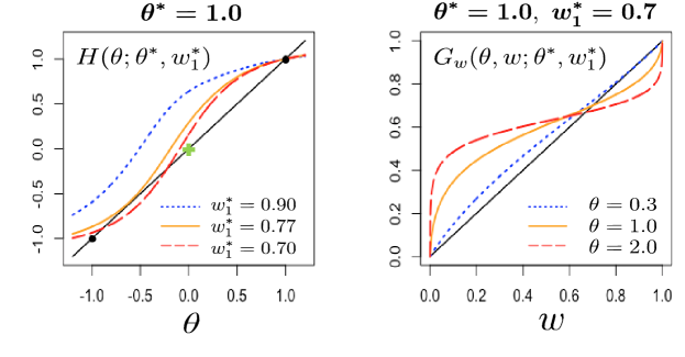
Figure 1: Left panel: we show the shape of iterative function $H(\theta;\theta^{*},w^{*}_{1})$ with $\theta^{*}=1$ and different values of $w^{*}_{1}\in\{0.9,0.77,0.7\}$. The green plus $+$ indicates the origin $(0,0)$ and the black points indicate the correct values $(\theta^{*},\theta^{*})$ and $(-\theta^{*},-\theta^{*})$. We observe that as $w^{*}_{1}$ increases, the number of fixed points goes down from $3$ to $2$ and finally to $1$. Further, when there exists more than one fixed point, there is one stable incorrect fixed point in $(-\theta^{*},0)$. Right panel: we show the shape of iterative function $G_{w}(\theta,w_{1};\theta^{*},w^{*}_{1})$ with $\theta^{*}=1,w^{*}_{1}=0.7$ and different values of $\theta\in\{0.3,1,2\}$. We observe that as $\theta$ increases, $G_{w}$ becomes from a concave function to a concave-convex function. Further, there are at most three fixed points and there is only one stable fixed point.

2.3 Roadmap of the proof for Theorem 2

Our first lemma, proved in Appendix B.1, confirms that if $\langle\rm{0},\boldsymbol{\theta}^{*}\rangle>0$, then $\langle\rm{t},\boldsymbol{\theta}^{*}\rangle>0$ for every $t$ and $w^{\langle t\rangle}_{1}\in(0.5,1)$. In other words, the estimates of the Population $\text{EM}_{2}$ remain in the correct hyperplane, and the weight moves in the right direction, too.

Lemma 1.

If $\langle\rm{0},\boldsymbol{\theta}^{*}\rangle>0$, we have $\langle\rm{t},\boldsymbol{\theta}^{*}\rangle>0,w^{\langle t\rangle}_{1}\in(0.5,1)$ for all $t\geq 1$. Otherwise, if $\langle\rm{0},\boldsymbol{\theta}^{*}\rangle<0$, we have $\langle\rm{t},\boldsymbol{\theta}^{*}\rangle<0,w^{\langle t\rangle}_{1}\in(0,0.5)$ for all $t\geq 1$.

On account of Lemma 1 and the invariance in (8), we can assume without loss of generality that $\langle\rm{t},\boldsymbol{\theta}^{*}\rangle>0$ and $w^{\langle t\rangle}_{1}\in(0.5,1)$ for all $t\geq 1$.

Let $d$ be the dimension of $\boldsymbol{\theta}^{*}$. We reduce the $d>1$ case to the $d=1$ case. This achieved by proving that the angle between the two vectors $\rm{t}$ and $\boldsymbol{\theta}^{*}$ is a decreasing function of $t$ and converges to $0$. The details appear in Appendix B.4. Hence, in the rest of this section we focus on the proof of Theorem 2 for $d=1$.

Let $g_{\theta}(\theta,w_{1})$ and $g_{w}(\theta,w_{1})$ be the shorthand for the two update functions $G_{\theta}$ and $G_{w}$ defined in (• ‣ 2.1) and (7) for a fixed $(\theta^{*},w^{*}_{1})$. To prove that $\{(\theta^{\langle t\rangle},w^{\langle t\rangle})\}$ converges to the fixed point $(\theta_{\star},w_{\star})$, we establish the following claims:

• There exists a set $S=(a_{\theta},b_{\theta})\times(a_{w},b_{w})\in\mathbb{R}^{2}$, where $a_{\theta},b_{\theta}\in\mathbb{R}\cup\{\pm\infty\}$ and $a_{w},b_{w}\in\mathbb{R}$, such that $S$ contains point $(\theta_{\star},w_{\star})$ and point $(g_{\theta}(\theta,w_{1}),g_{w}(\theta,w_{1}))\in S$ for all $(\theta,w_{1})\in S$. Further, $g_{\theta}(\theta,w_{1})$ is a non-decreasing function of $\theta$ for a given $w_{1}\in(a_{w},b_{w})$ and $g_{w}(\theta,w_{1})$ is a non-decreasing function of $w$ for a given $\theta\in(a_{\theta},b_{\theta})$,

• There is a reference curve $r\colon[a_{w},b_{w}]\rightarrow[a_{\theta},b_{\theta}]$ defined on $\bar{S}$ (the closure of $S$) such that:

  • $r$ is continuous, decreasing, and passes through point $(\theta_{\star},w_{\star})$, i.e., $r(w_{\star})=\theta_{\star}.$

  • Given $\theta\in(a_{\theta},b_{\theta})$, function $w\mapsto g_{w}(\theta,w)$ has a stable fixed point in $[a_{w},b_{w}]$. Further, any stable fixed point $w_{s}$ in $[a_{w},b_{w}]$ or fixed point $w_{s}$ in $(a_{w},b_{w})$ satisfies the following:

    • If $\theta<\theta_{\star}$ and $\theta\geq r(b_{w})$, then $r^{-1}(\theta)>w_{s}>w_{\star}$.

    • If $\theta=\theta_{\star}$, then $r^{-1}(\theta)=w_{s}=w_{\star}$.

    • If $\theta>\theta_{\star}$ and $\theta\leq r(a_{w})$, then $r^{-1}(\theta)<w_{s}<w_{\star}$.

  • Given $w\in[a_{w},b_{w}]$, function $\theta\mapsto g_{\theta}(\theta,w)$ has a stable fixed point in $[a_{\theta},b_{\theta}]$. Further, any stable fixed point $\theta_{s}$ in $[a_{\theta},b_{\theta}]$ or fixed point $\theta_{s}$ in $(a_{\theta},b_{\theta})$ satisfies the following:

    • If $w_{1}<w_{\star}$, then $r(w)>\theta_{s}>\theta_{\star}$.

    • If $w_{1}=w_{\star}$, then $r(w)=\theta_{s}=\theta_{\star}$.

    • If $w_{1}>w_{\star}$, then $r(w)<\theta_{s}<\theta_{\star}$.

We explain C.1 and C.2 in Figure 2. Heuristically, we expect $(\theta^{*},w^{*}_{1})$ to be the only fixed point of the mapping $(\theta,w)\mapsto(g_{\theta}(\theta,w),g_{w}(\theta,w))$, and that $(\theta^{\langle t\rangle},w^{\langle t\rangle})$ move toward this fixed point. Hence, we can prove the convergence of the iterates by showing certain geometric relationships between the curves of fixed points of the two functions. Hence, C.1 helps us to bound the iterates on the area that such nice geometric relations exist, and the reference curve $r$ and C.2 are the tools to help us mathematically characterizing the geometric relations shown in the figure. Indeed, the next lemma implies that $C.1$ and $C.2$ are sufficient to show the convergence to the right point $(\theta_{\star},w_{\star})$:

Lemma 2 (Proved in Appendix B.2.1).

Suppose continuous functions $g_{\theta}(\theta,w),g_{w}(\theta,w)$ satisfy $C.1$ and $C.2$, then there exists a continuous mapping $m\mathrel{\mathop{\mathchar 58\relax}}\bar{S}\rightarrow[0,\infty)$ such that $(\theta_{\star},w_{\star})$ is the only solution for $m(\theta,w)=0$ on $\bar{S}$, the closure of $S$ . Further, if we initialize $(\theta^{\langle 0\rangle},w^{\langle 0\rangle})$ in $S$, the sequence $\{(\theta^{\langle t\rangle},w^{\langle t\rangle})\}_{t\geq 0}$ defined by

$$\theta^{\langle t+1\rangle} = g_{\theta}(\theta^{\langle t\rangle},w^{\langle t\rangle}),\quad\text{and}\quad w^{\langle t+1\rangle}\ =\ g_{w}(\theta^{\langle t\rangle},w^{\langle t\rangle}),$$

satisfies that $m(\theta^{\langle t\rangle},w^{\langle t\rangle})\downarrow 0$, and therefore $(\theta^{\langle t\rangle},w^{\langle t\rangle})$ converges to $(\theta_{\star},w_{\star})$.

In our problem, we set $a_{w}=0.5,b_{w}=1,a_{\theta}=0,b_{\theta}=\infty$ and $(\theta_{\star},w_{\star})=(\theta^{*},w^{*}_{1})$. Then according to Lemma 1 and monotonic property of $g_{\theta}$ and $g_{w}$, C.1 is satisfied.

To show C.2, we first define the reference curve $r$ by

$$r(w_{1})\mathrel{\mathop{\mathchar 58\relax}}=\frac{w^{*}_{1}-w^{*}_{2}}{w_{1}-w_{2}}\theta^{*}\ =\ \frac{2w^{*}_{1}-1}{2w_{1}-1}\theta^{*},\quad\quad\forall w_{1}\in(0.5,1],w_{2}=1-w_{1}.$$ (9)

The claim C.2a holds by construction. To show C.2b, we establish an even stronger property of the weights update function $g_{w}(\theta,w)$: for any fixed $\theta>0$, the function $w_{1}\mapsto g_{w}(\theta,w_{1})$ has at most one other fixed point besides $w_{1}=0$ and $w_{1}=1$, and most importantly, it has only one unique stable fixed point. This is formalized in the following lemma.

Lemma 3 (Proved in Appendix B.2.2).

For all $\theta>0$, there are at most three fixed points for $g_{w}(\theta,w_{1})$ with respect to $w_{1}$. Further, there exists an unique stable fixed point $F_{w}(\theta)\in(0,1]$, i.e., (i) $F_{w}(\theta)=g_{w}(\theta,F_{w}(\theta))$ and (ii) for all $w_{1}\in(0,1)$, we have

$$g_{w}(\theta,w_{1})<w_{1}\Leftrightarrow w_{1}<F_{w}(\theta)\quad\text{and}\quad g_{w}(\theta,w_{1})>w_{1}\Leftrightarrow w_{1}>F_{w}(\theta).$$ (10)

We explain Lemma 3 in Figure 1. Note that, in the figure, we observe that $g_{w}$ is an increasing function with $g_{w}(\theta,0)=0$ and $g_{w}(\theta,1)=1$. Further, it is either a concave function, it is piecewise concave-then-convex. Hence, we know if $\partial g_{w}(\theta,w_{1})/\partial w_{1}|_{w_{1}=1}$ is at most $1$, the only stable fixed point is $w_{1}=1$, else if the derivative is larger than 1, there exists only one fixed point in (0,1) and it is the only stable fixed point. The complete proof for C.2b is shown in Appendix B.3.

The final step to apply Lemma 2 is to prove C2.c. However, $(\theta,w_{1})=((2w^{*}_{1}-1)\theta^{*},1)$ is a point on the reference curve $r$ and $\theta=(2w^{*}_{1}-1)\theta^{*}$ is a stable fixed point for $g_{\theta}(\theta,1)$. This violates C.2c. To address this issue, since we can characterize the shape and the number of fixed points for $g_{w}$, by typical uniform continuity arguments, we can find $\delta,\epsilon>0$ such that the adjusted reference curve $r_{adj}(w)\mathrel{\mathop{\mathchar 58\relax}}=r(w)-\epsilon\cdot\max(0,w-1+\delta)$ satisfies C.2a and C.2b. Then we can prove that the adjusted reference curve $r_{adj}(w)$ satisfies C2.c; see Appendix B.3.1.

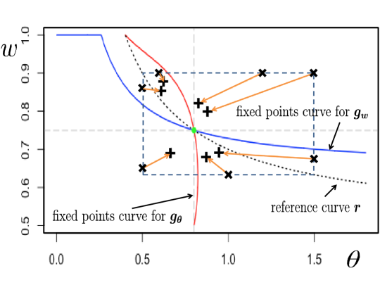
Figure 2: The functions $g_{\theta}$ and $g_{w}$ are shown with red and blue lines respectively. The green point at the intersections of the three curves is the correct convergence point $(\theta_{\star},w_{\star})$. The black dotted curve shows the reference curve $r$. The cross points $\times$ are the possible initializations and the plus points $+$ are the corresponding positions after the first iteration. By the geometric relations between the three curves, the iterations have to converge to $(\theta_{\star},w_{\star})$

3 Numerical results

In this section, we present numerical results that show the value of over-parameterization in some mixture models not covered by our theoretical results.

3.1 Setup

Our goal is to analyze the effect of the sample size, mixing weights, and the number of mixture components on the success of the two EM algorithms described in Section 2.1.

We implement EM for both Model 1 (where the weights are assumed to be known) and Model 2 (where the weights are not known), and run the algorithm multiple times with random initial mean estimates. We compare the two versions of EM by their (empirical) success probabilities, which we denote by $P_{1}$ and $P_{2}$, respectively. Success is defined in two ways, depending on whether EM is run with a finite sample, or with an infinite-size sample (i.e., the population analogue of EM).

When EM is run using a finite sample, we do not expect recover the $\boldsymbol{\theta}^{*}_{i}\in\mathbb{R}^{d}$ exactly. Hence, success is declared when the $\boldsymbol{\theta}^{*}_{i}$ are recovered up to some expected error, according to the following measure:

$$\text{error}\ =\ \min_{\pi\in\Pi}\lim_{t\rightarrow\infty}\sum_{i=1}^{k}w^{*}_{i}\|\rm{t}_{\pi(i)}-\boldsymbol{\theta}^{*}_{i}\|^{2},$$ (11)

where $\Pi$ is the set of all possible permutations on $\{1,\ldots,k\}$. We declare success if the error is at most $C_{\epsilon}/n$, where $C_{\epsilon}\mathrel{\mathop{\mathchar 58\relax}}=4\cdot\text{Tr}(\boldsymbol{W}^{*}\mathcal{I}^{-1}(\boldsymbol{\Theta}^{*}))$. Here, $\boldsymbol{W}^{*}$ is the diagonal matrix whose diagonal is $(w^{*}_{1},\ldots,w^{*}_{1},\dotsc,w^{*}_{k},\ldots,w^{*}_{k})\in\mathbb{R}^{kd}$, where each $w^{*}_{i}$ is repeated $d$ times, and $\mathcal{I}(\boldsymbol{\Theta}^{*})$ is the Fisher Information at the true value $\boldsymbol{\Theta}^{*}\mathrel{\mathop{\mathchar 58\relax}}=(\boldsymbol{\theta}^{*}_{1},\dotsc,\boldsymbol{\theta}^{*}_{k})$. We adopt this criteria since it is well known that the MLE asymptotically converges to $\mathcal{N}(\theta^{*},\mathcal{I}^{-1}(\boldsymbol{\Theta}^{*})/n)$. Thus, constant $4\approx 1.96^{2}$ indicates an approximately $95\%$ coverage.

When EM is run using an infinite-size sample, we declare EM successful when the error defined in (11) is at most $10^{-7}$.

3.2 Mixtures of two Gaussians

We first consider mixtures of two Gaussians in one dimension, i.e., $\theta^{*}_{1},\theta^{*}_{2}\in\mathbb{R}$. Unlike in our theoretical analysis, the mixture components are not constrained to be symmetric about the origin. For simplicity, we always let $\theta^{*}_{1}=0$, but this information is not used by EM. Further, we consider sample size $n\in\{1000,\infty\}$, separation $\theta^{*}_{2}=|\theta^{*}_{2}-\theta^{*}_{1}|\in\{1,2,4\}$, and mixing weight $w^{*}_{1}\in\{0.52,0.7,0.9\}$; this gives a total of 18 cases. For each case, we run EM with $2500$ random initializations and compute the empirical probability of success. When $n=1000$, the initial mean parameter is chosen uniformly at random from the sample. When $n=\infty$, the initial mean parameter is chosen uniformly at random from the rectangle $[-2,\theta^{*}_{2}+2]\times[-2,\theta^{*}_{2}+2]$.

A subset of the success probabilities are shown in Table 1; see Appendix F for the full set of results. Our simulations lead to the following empirical findings about the behavior of EM on data from well-separated mixtures ($|\theta^{*}_{1}-\theta^{*}_{2}|\geq 1$). First, for $n=\infty$, EM for Model 2 finds the MLE almost always ($P_{2}=1$), while EM for Model 1 only succeeds about half the time ($P_{1}\approx 0.5$). Second, for smaller $n$, EM for Model 2 still has a higher chance of success than EM for Model 1, except when the weights $w^{*}_{1}$ and $w^{*}_{2}$ are almost equal. When $w^{*}_{1}\approx w^{*}_{2}\approx 1/2$, the bias in Model 1 is not big enough to stand out from the error due to the finite sample, and hence Model 1 is more preferable. Notably, unlike the special model in (2), highly unbalanced weights do not help EM for Model 1 due to the lack of the symmetry of the component means (i.e., we may have $\theta^{*}_{1}+\theta^{*}_{2}\neq 0$).

We conclude that over-parameterization helps EM if the two mixture components are well-separated and the mixing weights are not too close.

3.3 Mixtures of three or four Gaussians

We now consider a setup with mixtures of three or four Gaussians. Specifically, we consider the following four cases, each using a larger sample size of $n=2000$:

• Case 1, mixture of three Gaussians on a line: $\boldsymbol{\theta}^{*}_{1}=(-3,0)$, $\boldsymbol{\theta}^{*}_{2}=(0,0)$, $\boldsymbol{\theta}^{*}_{3}=(2,0)$ with weights $w^{*}_{1}=0.5,w^{*}_{2}=0.3,w^{*}_{3}=0.2$.

• Case 2, mixture of three Gaussians on a triangle: $\boldsymbol{\theta}^{*}_{1}=(-3,0)$, $\boldsymbol{\theta}^{*}_{2}=(0,2)$, $\boldsymbol{\theta}^{*}_{3}=(2,0)$ with weights $w^{*}_{1}=0.5,w^{*}_{2}=0.3,w^{*}_{3}=0.2$.

• Case 3, mixture of four Gaussians on a line: $\boldsymbol{\theta}^{*}_{1}=(-3,0)$, $\boldsymbol{\theta}^{*}_{2}=(0,0)$, $\boldsymbol{\theta}^{*}_{3}=(2,0)$, $\boldsymbol{\theta}^{*}_{4}=(5,0)$ with weights $w^{*}_{1}=0.35,w^{*}_{2}=0.3,w^{*}_{3}=0.2,w^{*}_{4}=0.15$.

• Case 4, mixture of four Gaussians on a trapezoid: $\boldsymbol{\theta}^{*}_{1}=(-3,0)$, $\boldsymbol{\theta}^{*}_{2}=(-1,2)$, $\boldsymbol{\theta}^{*}_{3}=(2,0)$, $\boldsymbol{\theta}^{*}_{4}=(2,2)$ with weights $w^{*}_{1}=0.35,w^{*}_{2}=0.3,w^{*}_{3}=0.2,w^{*}_{4}=0.15$.

The other aspects of the simulations are the same as in the previous subsection.

The results are presented in Table 1. From the table, we confirm that EM for Model 2 (with unknown weights) has a higher success probability than EM for Model 1 (with known weights). Therefore, over-parameterization helps in all four cases.

3.4 Explaining the disparity

As discussed in Section 2.2, the performance EM algorithm with unknown weights does not depend on the ordering of the initialization means. We conjuncture that in general, this property that is a consequence of over-parameterization leads to the boost that is observed in the performance of EM with unknown weights.

We support this conjecture by revisiting the previous simulations with a different way of running EM for Model 1. For each set of $k$ vectors selected to be used as initial component means, we run EM $k!$ times, each using a different one-to-one assignment of these vectors to initial component means. We measure the empirical success probability $P_{3}$ based on the lowest observed error among these $k!$ runs of EM. The results are presented in Table 3 in Appendix F. In general, we observe $P_{3}\gtrsim P_{2}$ for all cases we have studied, which supports our conjecture. However, this procedure is generally more time-consuming than EM for Model 2 since $k!$ executions of EM are required.

Success probabilities for mixtures of two Gaussians (Section 3.2)

Separation	Sample size	$w^{*}_{1}=0.52$	$w^{*}_{1}=0.7$	$w^{*}_{1}=0.9$
$\theta^{*}_{2}-\theta^{*}_{1}=2$	$n=1000$	0.799  /  0.500	0.497  /  0.800	0.499  /  0.899
	$n=\infty$	0.504  /  1.000	0.514  /  1.000	0.506  /  1.000

Success probabilities for mixtures of three or four Gaussians (Section 3.3)

Case 1	Case 2	Case 3	Case 4
0.164  /  0.900	0.167  /  1.000	0.145  /  0.956	0.159  /  0.861

Table 1: Success probabilities for EM on Model 1 and Model 2 (denoted $P_{1}$ and $P_{2}$, respectively), reported as ${\color[rgb]{1,0,0}P_{1}}\;/\;{\color[rgb]{0,0,1}P_{2}}$.

Acknowledgements

DH and JX were partially supported by NSF awards DMREF-1534910 and CCF-1740833, and JX was also partially supported by a Cheung-Kong Graduate School of Business Fellowship. We thank Jiantao Jiao for a helpful discussion about this problem.

Appendix A Proof of Theorem 1

Let us define $h(\theta,w^{*}_{1})\mathrel{\mathop{\mathchar 58\relax}}=H(\theta;\theta^{*},w^{*}_{1})$. First, it is straightforward to show that

$$h(0,0.5)=0,$$

and

• $h(\theta,0.5)$ is concave for $\theta\geq 0$ and $h(\theta^{*},0.5)=\theta^{*}$.

• $h(\theta,0.5)$ is convex for $\theta\leq 0$ and $h(-\theta^{*},0.5)=-\theta^{*}$.

Hence, we have

$$h(\theta,0.5)-\theta = \left\{\begin{aligned} &>0,&&\theta\in(-\infty,-\theta^{*})\bigcup(0,\theta^{*})\\ &=0,&&\theta=-\theta^{*},0,\theta^{*}\\ &<0,&&\theta\in(-\theta^{*},0)\bigcup(\theta^{*},\infty)\end{aligned}\right.$$ (12)

Therefore, if we can show that the curve of $h(\theta,w^{*}_{1})$ is strictly above the curve $h(\theta,0.5)$ for all $w^{*}_{1}>0.5$ and $\theta<\theta^{*}$, i.e.,

$$h(\theta,w^{*}_{1}) > h(\theta,0.5),\quad\quad\forall w^{*}_{1}>0.5,\theta<\theta^{*},$$ (13)

then by (12), we have

$$h(\theta,w^{*}_{1})-\theta > h(\theta,0.5)-\theta\ \geq\ 0,\quad\quad\forall w^{*}_{1}>0.5,\theta\leq-\theta^{*}.$$ (14)

Further, since $h$ is continuous, we know there exists $\delta>0$ and $\theta_{\delta}$, such that

$$h(\theta_{\delta},w^{*}_{1})\ <\ \theta_{\delta},\quad\forall w^{*}_{1}\in[0.5,0.5+\delta].$$

Hence, with (14) and continuity of function $h(\theta,w^{*}_{1})-\theta$, we know for each $w^{*}_{1}\in(0.5,0.5+\delta]$, there exists $\theta_{w}\in(-\theta^{*},0)$ (the smallest fixed point) such that

$$h(\theta_{w},w^{*}_{1}) = \theta_{w}\quad\text{and}\quad h(\theta,w^{*}_{1})\ >\ \theta,\quad\quad\forall\theta\in(-\infty,\theta_{w}).$$

Therefore, if we initialize $\theta^{\langle 0\rangle}\leq-\theta^{*}$, the EM estimate will converge to $\theta_{w}$. Hence, our final step is to show (14) which is proved in the following lemma:

Lemma 4 (Proved in Appendix E.1).

For all $w^{*}_{1}\neq 0.5$, we have

$$h(\theta,w^{*}_{1}) > h(\theta,0.5),\quad\quad\forall\theta<\theta^{*},$$ (15)

and for all $w^{*}_{1}\in[0,1]$, we have

$$0\ \leq\ \frac{\partial h(\theta,w^{*}_{1})}{\partial\theta}\ \leq\ e^{-\frac{(\theta^{*})^{2}}{2}}\ <\ 1,\quad\quad\forall\theta\geq\theta^{*}.$$ (16)

In fact, by Lemma 4, (12) and the fact $h(\theta^{*},w)\equiv\theta^{*}$, it is straightforward to show the following corollary

Corollary 1.

For all $w^{*}_{1}\in[0,1]$, $h(\theta,w^{*}_{1})$ has only one fixed point (a stable fixed point) in $(0,\infty)$, which is $\theta=\theta^{*}$.

Appendix B Proof of Theorem 2

From the discussion in Section 2.2, we just need to prove Theorem 2 for $w^{*}_{1}>0.5$. We use the following the strategy to prove Theorem 2.

1. Prove Lemma 1 (see Section 2.3) and therefore WLOG, we can safely assume $\langle\rm{t},\boldsymbol{\theta}^{*}\rangle>0$ and $w^{\langle t\rangle}>0.5$ for all $t>0$.

2. Prove Theorem 2 when the mean parameters $\theta^{*}_{i}$ is in one dimension.

3. Show that we can reduce the multi-dimensional problem into the one dimensional one.

4. Show geometric convergence by proving an attraction basin around $(\boldsymbol{\theta}^{*},w^{*}_{1})$.

Each one of the steps is proved in the following subsections in order.

B.1 Proof of Lemma 1

First it is clear that $w^{\langle t\rangle}_{1}\in(0,1)$. Hence, due to our initialization setting $w^{\langle 0\rangle}_{1}=w^{\langle 0\rangle}_{2}=0.5$, we just need to show

• For all $\langle\boldsymbol{\theta},\boldsymbol{\theta}^{*}\rangle>0,w_{1}\in[0.5,1)$, we have

  $$\langle G_{\theta}(\boldsymbol{\theta},w_{1};\boldsymbol{\theta}^{*},w^{*}_{1}),\boldsymbol{\theta}^{*}\rangle\ >\ 0\quad\text{and}\quad G_{w}(\boldsymbol{\theta},w_{1};\boldsymbol{\theta}^{*},w^{*}_{1})\ >\ 0.5.$$ (17)

• For all $\langle\boldsymbol{\theta},\boldsymbol{\theta}^{*}\rangle<0,w_{1}\in(0,0.5]$, we have

  $$\langle G_{\theta}(\boldsymbol{\theta},w_{1};\boldsymbol{\theta}^{*},w^{*}_{1}),\boldsymbol{\theta}^{*}\rangle\ <\ 0\quad\text{and}\quad G_{w}(\boldsymbol{\theta},w_{1};\boldsymbol{\theta}^{*},w^{*}_{1})\ <\ 0.5.$$ (18)

and then by a simple induction argument, it is straightforward to show Lemma 1 holds. Moreover, let $w_{2}=1-w_{1}$ and note that the symmetric property of $G_{\theta}$ and $G_{w}$, i.e.,

$$G_{\theta}(\boldsymbol{\theta},w_{1};\boldsymbol{\theta}^{*},w^{*}_{1})+G_{\theta}(-\boldsymbol{\theta},w_{2};\boldsymbol{\theta}^{*},w^{*}_{1}) = 0$$

$$G_{w}(\boldsymbol{\theta},w_{1};\boldsymbol{\theta}^{*},w^{*}_{1})+G_{w}(-\boldsymbol{\theta},w_{2};\boldsymbol{\theta}^{*},w^{*}_{1}) = 1.$$

Hence, we just need to show (17) holds. Since for any orthogonal matrices $\boldsymbol{V}$, we have

$$\langle G_{\theta}(\boldsymbol{\theta},w_{1};\boldsymbol{\theta}^{*},w^{*}_{1}),\boldsymbol{\theta}^{*}\rangle = \langle G_{\theta}(\boldsymbol{V}\boldsymbol{\theta},w_{1};\boldsymbol{V}\boldsymbol{\theta}^{*},w^{*}_{1}),\boldsymbol{V}\theta^{*}\rangle$$

$$G_{w}(\boldsymbol{\theta},w_{1};\boldsymbol{\theta}^{*},w^{*}_{1}) = G_{w}(\boldsymbol{V}\boldsymbol{\theta},w_{1};\boldsymbol{V}\boldsymbol{\theta}^{*},w^{*}_{1})$$

Hence, the claim made in (17) and (18) is invariant to rotation of the coordinates. Hence, WLOG, we assume that $\boldsymbol{\theta}=(\|\boldsymbol{\theta}\|,0,0,\ldots,0)$ and $\boldsymbol{\theta}^{*}=(\theta^{*}_{\parallel},\theta^{*}_{\perp},0,\ldots,0)$ with $\theta^{*}_{\parallel}>0$. Let us first show $G_{w}(\boldsymbol{\theta},w;\boldsymbol{\theta}^{*},w^{*}_{1})\ >\ 0.5$. It is straightforward to show that

$$G_{w}(\boldsymbol{\theta},w_{1};\boldsymbol{\theta}^{*},w^{*}_{1}) = \int\frac{w_{1}e^{y\|\theta\|}}{w_{1}e^{y\|\theta\|}+w_{2}e^{-y\|\theta\|}}\left(w^{*}_{1}\phi(y-\theta^{*}_{\parallel})+w^{*}_{2}\phi(y+\theta^{*}_{\parallel})\right)\operatorname{d\!}y$$

$$=\mathrel{\mathop{\mathchar 58\relax}} g_{w}(\|\theta\|,w_{1};\theta^{*}_{\parallel},w^{*}_{1}),$$

where $\phi(x)$ denotes the pdf for $d^{\prime}-$dimensional standard Gaussian if $x\in\mathbb{R}^{d^{\prime}}$. Hence, we just need to show that

$$g_{w}(\theta,w_{1};\theta^{*},w^{*}_{1})\ >\ 0.5,\quad\forall w_{1}\in[0.5,1),w^{*}_{1}\in(0.5,1),\theta>0,\theta^{*}>0.$$ (19)

Note that

$$\frac{\partial g_{w}(\theta,w_{1};\theta^{*},w^{*}_{1})}{\partial w_{1}} = \int\frac{1}{\left(w_{1}e^{y\theta}+w_{2}e^{-y\theta}\right)^{2}}\left(w^{*}_{1}\phi(y-\theta^{*})+w^{*}_{2}\phi(y+\theta^{*})\right)\operatorname{d\!}y\ >\ 0.$$

Hence, we just need to show $g_{w}(\theta,0.5;\theta^{*},w^{*}_{1})>0.5$. Note that

$$g_{w}(\theta,0.5;\theta^{*},w^{*}_{1})-0.5 = \int\frac{e^{y\theta}}{e^{y\theta}+e^{-y\theta}}\left(w^{*}_{1}\phi(y-\theta^{*})+w^{*}_{2}\phi(y+\theta^{*})\right)\operatorname{d\!}y-0.5$$

$$= \int\frac{e^{y\theta}-e^{-y\theta}}{2(e^{y\theta}+e^{-y\theta})}\left(w^{*}_{1}\phi(y-\theta^{*})+w^{*}_{2}\phi(y+\theta^{*})\right)\operatorname{d\!}y$$

$$= \int_{y\geq 0}\phi(y)e^{-\frac{(\theta^{*})^{2}}{2}}\cdot\left(\frac{(2w^{*}_{1}-1)\left(\cosh_{y}(\theta^{*}+\theta)-\cosh_{y}(\theta^{*}-\theta)\right)}{2\cosh_{y}(\theta)}\right)\operatorname{d\!}y$$

$$> 0,$$

where $\cosh_{y}(x)=\frac{1}{2}(e^{yx}+e^{-yx})$. Hence, (19) holds. Now we just need to show $\langle G_{\theta}(\boldsymbol{\theta},w_{1};\boldsymbol{\theta}^{*},w^{*}_{1}),\boldsymbol{\theta}^{*}\rangle>0$. It is straightforward to show that all components of $G_{\theta}(\boldsymbol{\theta},w_{1};\boldsymbol{\theta}^{*},w^{*}_{1})$ are $0$ except for the first two components denoted as $\tilde{\theta}_{1}$ and $\tilde{\theta}_{2}$. For the second component $\tilde{\theta}_{2}$, we have

$$\tilde{\theta}_{2} = \theta^{*}_{\perp}\int\frac{w_{1}e^{y\|\theta\|}-w_{2}e^{-y\|\theta\|}}{w_{1}e^{y\|\theta\|}+w_{2}e^{-y\|\theta\|}}\left(w^{*}_{1}\phi(y-\theta^{*}_{\parallel})-w^{*}_{2}\phi(y+\theta^{*}_{\parallel})\right)\operatorname{d\!}y$$ (20)

$$=\mathrel{\mathop{\mathchar 58\relax}} \theta^{*}_{\perp}\cdot s(\|\theta\|,w_{1};\theta^{*}_{\parallel},w^{*}_{1}),$$

and for the first component $\tilde{\theta}_{1}$, we have

$$\tilde{\theta}_{1} = \theta^{*}_{\parallel}\int\frac{w_{1}e^{y\|\theta\|}-w_{2}e^{-y\|\theta\|}}{w_{1}e^{y\|\theta\|}+w_{2}e^{-y\|\theta\|}}\left(w^{*}_{1}\phi(y-\theta^{*}_{\parallel})-w^{*}_{2}\phi(y+\theta^{*}_{\parallel})\right)\operatorname{d\!}y$$ (21)

$$+\int\frac{w_{1}e^{y\|\theta\|}-w_{2}e^{-y\|\theta\|}}{w_{1}e^{y\|\theta\|}+w_{2}e^{-y\|\theta\|}}\left(w^{*}_{1}(y-\theta^{*}_{\parallel})\phi(y-\theta^{*}_{\parallel})+w^{*}_{2}(y+\theta^{*}_{\parallel})\phi(y+\theta^{*}_{\parallel})\right)\operatorname{d\!}y$$

$$\stackrel{{\scriptstyle(a)}}{{=}} \theta^{*}_{\parallel}\cdot s(\|\theta\|,w_{1};\theta^{*}_{\parallel},w^{*}_{1})+\|\theta\|\int\frac{4w_{1}w_{2}}{\left(w_{1}e^{y\|\theta\|}+w_{2}e^{-y\|\theta\|}\right)^{2}}\left(w^{*}_{1}\phi(y-\theta^{*}_{\parallel})+w^{*}_{2}\phi(y+\theta^{*}_{\parallel})\right)\operatorname{d\!}y$$

$$> \theta^{*}_{\parallel}\cdot s(\|\theta\|,w_{1};\theta^{*}_{\parallel},w^{*}_{1}),$$

where equation (a) holds due to partial integration. Hence, by (20) and (21) and $\theta^{*}_{\parallel}>0$, we have

$$\langle G_{\theta}(\boldsymbol{\theta},w_{1};\boldsymbol{\theta}^{*},w^{*}_{1}),\boldsymbol{\theta}^{*}\rangle > \|\theta^{*}\|^{2}\cdot s(\|\theta\|,w_{1};\theta^{*}_{\parallel},w^{*}_{1}).$$

Hence, we just need to show

$$s(\theta,w_{1};\theta^{*},w^{*}_{1}) > 0,\quad\forall\theta>0,w_{1}\in[0.5,1],\theta^{*}>0,w^{*}_{1}\in(0.5,1).$$ (22)

For $w_{1}=0.5$, by (20), we have

$$s(\theta,0.5;\theta^{*},w^{*}_{1}) = \int\frac{e^{y\theta}-e^{-y\theta}}{e^{y\theta}+e^{-y\theta}}\left(w^{*}_{1}\phi(y-\theta^{*})-w^{*}_{2}\phi(y+\theta^{*})\right)\operatorname{d\!}y$$ (23)

$$= \int_{y\geq 0}\frac{e^{y\theta}-e^{-y\theta}}{e^{y\theta}+e^{-y\theta}}\phi(y)e^{-\frac{(\theta^{*})^{2}}{2}}\left(e^{y\theta^{*}}-e^{-y\theta^{*}}\right)\operatorname{d\!}y\ >\ 0.$$

For $w_{1}\in(0.5,1]$, by (20) and taking derivative with respect to $w^{*}_{1}$, we have

$$\frac{\partial s(\theta,w_{1};\theta^{*},w^{*}_{1})}{\partial w^{*}_{1}} = \int\frac{w_{1}e^{y\theta}-w_{2}e^{-y\theta}}{w_{1}e^{y\theta}+w_{2}e^{-y\theta}}\left(\phi(y-\theta^{*})+\phi(y+\theta^{*})\right)\operatorname{d\!}y$$

$$= \int_{y\geq 0}\frac{2(w_{1}^{2}-w^{2}_{2})}{\left(w_{1}e^{y\theta}+w_{2}e^{-y\theta}\right)\left(w_{1}e^{-y\theta}+w_{2}e^{y\theta}\right)}\left(\phi(y-\theta^{*})+\phi(y+\theta^{*})\right)\operatorname{d\!}y$$

$$> 0.$$

Hence, we just need to show

$$s(\theta,w_{1};\theta^{*},0.5) \geq 0,\quad\forall\theta>0,w_{1}\in(0.5,1],\theta^{*}>0.$$ (24)

Note that

$$2s(\theta,w_{1};\theta^{*},0.5) = \int\frac{w_{1}e^{y\theta}-w_{2}e^{-y\theta}}{w_{1}e^{y\theta}+w_{2}e^{-y\theta}}\left(\phi(y-\theta^{*})-\phi(y+\theta^{*})\right)\operatorname{d\!}y$$

$$= \int_{y\geq 0}\frac{w_{1}w_{2}(e^{2y\theta}-e^{-2y\theta})}{\left(w_{1}e^{y\theta}+w_{2}e^{-y\theta}\right)\left(w_{1}e^{-y\theta}+w_{2}e^{y\theta}\right)}\left(\phi(y-\theta^{*})-\phi(y+\theta^{*})\right)\operatorname{d\!}y$$

$$\geq 0.$$

Hence, we have (24) holds. Combine with (23), we have (22) holds which completes the proof of this lemma.

B.2 Proof of Theorem 2 in one dimension

We filled out the proofs that have left out in Section 2.3, namely Lemma 2, Lemma 3 and C.2c.

B.2.1 Proof of Lemma 2

Based on $(\theta_{\star},w_{\star})$, we divide the region of $S-\{(\theta_{\star},w_{\star})\}$ into 8 pieces:

• $R_{1}=\{(\theta,w)\in S\mathrel{\mathop{\mathchar 58\relax}}\theta\in[\theta_{\star},\min\{r(a_{w}),b_{\theta}\}),w\in(a_{w},w_{\star}]\}-\{(\theta_{\star},w_{\star})\}$.

• $R_{2}=\{(\theta,w)\in S\mathrel{\mathop{\mathchar 58\relax}}\theta\in[\theta_{\star},\min\{r(a_{w}),b_{\theta}\}),w\in[w_{\star},b_{w})\}-\{(\theta_{\star},w_{\star})\}$.

• $R_{3}=\{(\theta,w)\in S\mathrel{\mathop{\mathchar 58\relax}}\theta\in(\max\{r(b_{w}),a_{\theta}\},\theta_{\star}],w\in(a_{w},w_{\star}]\}-\{(\theta_{\star},w_{\star})\}$.

• $R_{4}=\{(\theta,w)\in S\mathrel{\mathop{\mathchar 58\relax}}\theta\in(\max\{r(b_{w}),a_{\theta}\},\theta_{\star}],w\in[w_{\star},b_{w})\}-\{(\theta_{\star},w_{\star})\}$.

• $R_{5}=\{(\theta,w)\in S\mathrel{\mathop{\mathchar 58\relax}}\theta\leq r(b_{w}),w\in(a_{w},w_{\star}]\}$.

• $R_{6}=\{(\theta,w)\in S\mathrel{\mathop{\mathchar 58\relax}}\theta\leq r(b_{w}),w\in[w_{\star},b_{w})\}$.

• $R_{7}=\{(\theta,w)\in S\mathrel{\mathop{\mathchar 58\relax}}\theta\geq r(a_{w}),w\in(a_{w},w_{\star}]\}$.

• $R_{8}=\{(\theta,w)\in S\mathrel{\mathop{\mathchar 58\relax}}\theta\geq r(a_{w}),w\in[w_{\star},b_{w})\}$.

Note that region $R_{5}$ to $R_{8}$ may not exists depending on the range of $r(w)$. Next, due to C.2a, we know the reference curve only crosses region $R_{1}$ and $R_{4}$. Note that $r^{-1}(\theta)$ exists on the regions $R_{1},R_{2},R_{3}$ and $R_{4}$. Hence, based on the points are above or below the reference curve $r$, we can further divide the region $R_{1}$ and $R_{4}$ into 4 pieces:

• $R_{11}=\{(\theta,w)\in R_{1}\mathrel{\mathop{\mathchar 58\relax}}r^{-1}(\theta)\leq w\}$.

• $R_{12}=\{(\theta,w)\in R_{1}\mathrel{\mathop{\mathchar 58\relax}}r^{-1}(\theta)\geq w\}$.

• $R_{41}=\{(\theta,w)\in R_{4}\mathrel{\mathop{\mathchar 58\relax}}w\leq r^{-1}(\theta)\}$.

• $R_{42}=\{(\theta,w)\in R_{4}\mathrel{\mathop{\mathchar 58\relax}}w\geq r^{-1}(\theta)\}$.

Now let’s define $m\mathrel{\mathop{\mathchar 58\relax}}S\rightarrow[0,\infty)$ based on the following 10 regions

$$\{R_{11},R_{12},R_{2},R_{3},R_{41},R_{42},R_{5},R_{6},R_{7},R_{8}\}\mathrel{\mathop{\mathchar 58\relax}}$$

• If $(\theta,w)\in R_{11}$, $m(\theta,w)=(w_{\star}-w)(r(w)-\theta_{\star})$, which is the area of the rectangle $D(\theta,w)$ given by $(\theta_{\star},w_{\star}),(r(w),w)$.

• If $(\theta,w)\in R_{12}$, $m(\theta,w)=(w_{\star}-r^{-1}(\theta))(\theta-\theta_{\star})$, which is the area of the rectangle $D(\theta,w)$ given by $(\theta_{\star},w_{\star}),(\theta,r^{-1}(\theta))$.

• If $(\theta,w)\in R_{2}$, $m(\theta,w)=(w-r^{-1}(\theta))(\theta-r(w))$, which is the area of the rectangle $D(\theta,w)$ given by $(r(w),r^{-1}(\theta)),(\theta,w)$.

• If $(\theta,w)\in R_{3}$, $m(\theta,w)=(r^{-1}(\theta)-w)(r(w)-\theta)$, which is the area of the rectangle $D(\theta,w)$ given by $(r(w),r^{-1}(\theta)),(\theta,w)$.

• If $(\theta,w)\in R_{41}$, $m(\theta,w)=(r^{-1}(\theta)-w_{\star})(\theta_{\star}-\theta)$, which is the area of the rectangle $D(\theta,w)$ given by $(\theta_{\star},w_{\star}),(\theta,r^{-1}(\theta))$.

• If $(\theta,w)\in R_{42}$, $m(\theta,w)=(w-w_{\star})(\theta_{\star}-r(w))$, which is the area of the rectangle $D(\theta,w)$ given by $(\theta_{\star},w_{\star}),(r(w),w)$.

• If $(\theta,w)\in R_{5}$, $m(\theta,w)=(b_{w}-w)(r(w)-\theta)$, which is the area of the rectangle $D(\theta,w)$ given by $(r(w),b_{w}),(\theta,w)$.

• If $(\theta,w)\in R_{6}$, $m(\theta,w)=(b_{w}-w_{\star})(\theta_{\star}-\theta)$, which is the area of the rectangle $D(\theta,w)$ given by $(\theta,b_{w}),(\theta_{\star},w_{\star})$.

• If $(\theta,w)\in R_{7}$, $m(\theta,w)=(w_{\star}-a_{w})(\theta-\theta_{\star})$, which is the area of the rectangle $D(\theta,w)$ given by $(\theta_{\star},w_{\star}),(\theta,a_{w})$.

• If $(\theta,w)\in R_{8}$, $m(\theta,w)=(w-a_{w})(\theta-r(w))$, which is the area of the rectangle $D(\theta,w)$ given by $(r(w),a_{w}),(\theta,w)$.

It is straightforward to show that function $m$ is a continuous function by checking the boundary and continuity of the reference function $r$. Further, $(\theta_{\star},w_{\star})$ is indeed the only solution for $m(\theta,w)=0$. Moreover, our construction of the rectangle $D$ makes sure that

$$\text{If~{}}(\tilde{\theta},\tilde{w})\text{~{}is strictly inside~{}}D(\theta,w),\ \text{~{}then~{}}D(\tilde{\theta},\tilde{w})\subsetneq D(\theta,w).$$ (25)

Next, we shall discuss the movement of the iterates from point $(\theta^{\langle t\rangle},w^{\langle t\rangle})$ to point $(\theta^{\langle t+1\rangle},w^{\langle t+1\rangle})$. For a given $w^{\langle t\rangle}\in[a_{w},b_{w}]$, consider all the fixed points $\mathcal{V}$ in $[a_{\theta},b_{\theta}]$ for $g_{\theta}(\theta,w)$ with respect to $\theta$. Then, for any $\theta^{\langle t\rangle}\in(a_{\theta},b_{\theta})$, it should be inside an interval defined by $[q_{1},q_{2}]$ where $q_{1},q_{2}\in\mathcal{V}\bigcup\{a_{\theta},b_{\theta}\}$ and at least one of $q_{1}$ or $q_{2}$ is either a stable fixed point or one of $a_{\theta},b_{\theta}$. Further, since $g_{\theta}(\theta,w)$ is a non-decreasing function of $\theta$ and $(\theta^{\langle t+1\rangle},w^{\langle t+1\rangle})\in S$, we know $\theta^{\langle t+1\rangle}=g_{\theta}(\theta^{\langle t\rangle},w^{\langle t\rangle})\in[q_{1},q_{2}]$ as well. Hence, comparing to the previous iteration $\theta^{\langle t\rangle}$, $\theta^{\langle t+1\rangle}=g_{\theta}(\theta^{\langle t\rangle},w^{\langle t\rangle})$ should (i) stay at a fixed point, i.e., $q_{1}$ or $q_{2}$ or (ii) move towards a stable fixed point $q_{i}$ or $a_{\theta},b_{\theta}$. Further, if $\theta^{\langle t+1\rangle}$ moves towards $a_{\theta}$ or $b_{\theta}$, then $a_{\theta}$ or $b_{\theta}$ has to be a stable fixed point as well. In other words, suppose $\theta^{\langle t+1\rangle}$ move towards $a_{\theta}$ and $a_{\theta}$ is not a stable fixed point. Then $a_{\theta}$ is not a fixed point as well and there exists a constant $c>0$ such that $\lim_{\theta\rightarrow a_{\theta}}g_{\theta}(\theta,w^{\langle t\rangle})\leq a_{\theta}-c$. Hence by choosing $\theta$ close enough to $a_{\theta}$, we know $g_{\theta}(\theta,w)<a_{\theta}$ which contradicts C.1. Now, by C.2b, C.2c and discussing which region $(\theta,w)$ belongs to, we can prove

$$\text{Point~{}}(\theta^{\langle t+1\rangle},w^{\langle t+1\rangle})\text{~{}is strictly inside~{}}D(\theta^{\langle t\rangle},w^{\langle t\rangle})\quad\text{and}\quad m(\theta^{\langle t+1\rangle},w^{\langle t+1\rangle}) < m(\theta^{\langle t\rangle},w^{\langle t\rangle}).$$

and

$$\text{If~{}}(\theta^{\langle t\rangle},w^{\langle t\rangle})\in R_{1}\bigcup R_{2}\bigcup R_{3}\bigcup R_{4},\quad\text{then~{}}(\theta^{\langle t+1\rangle},w^{\langle t+1\rangle})\in R_{1}\bigcup R_{2}\bigcup R_{3}\bigcup R_{4}.$$ (27)

Note that depending on the regions, there are total 10 cases. But for simplicity, we show the proof for two cases: $R_{11}$ and $R_{6}$ and leave the rest of the cases to the readers. For the first example, if point $(\theta^{\langle t\rangle},w^{\langle t\rangle})\in R_{11}$, then we know there exists a fixed point $\theta_{s}\in[\theta_{\star},b_{\theta}]$ for $g_{\theta}$ and $w_{s}\in[a_{w},w_{\star}]$ for $g_{w}$ such that $\theta^{\langle t+1\rangle}=g_{\theta}(\theta^{\langle t\rangle},w^{\langle t\rangle})$ lies in between $\theta^{\langle t\rangle}$ and $\theta_{s}$, and $w^{\langle t+1\rangle}=g_{w}(\theta^{\langle t\rangle},w^{\langle t\rangle})$ lies in between $w^{\langle t\rangle}$ and $w_{s}$. Hence $(\theta^{\langle t+1\rangle},w^{\langle t+1\rangle})$ can only stay in $R_{1}$ which proves (27) for the case $(\theta^{\langle t\rangle},w^{\langle t\rangle})\in R_{11}$. Further, we have

$$|g_{\theta}(\theta^{\langle t\rangle},w^{\langle t\rangle})-\theta_{s}| \leq |\theta^{\langle t\rangle}-\theta_{s}|,$$ (28)

$$|g_{w}(\theta^{\langle t\rangle},w^{\langle t\rangle})-w_{s}| \leq |w^{\langle t\rangle}-w_{s}|,$$ (29)

where equality (28)/(29) holds if and only if $\theta^{\langle t\rangle}=\theta_{s}$/$w^{\langle t\rangle}=w_{s}$. Hence, by C.2, we have

• If $\theta^{\langle t\rangle}=\theta_{\star}$, then $w^{\langle t\rangle}<w_{\star}$. Hence we have $\theta_{s}\in(\theta_{\star},r(w^{\langle t\rangle}))$ and $w_{s}=w_{\star}$. and therefore, (29) is strict inequality. Hence, $w^{\langle t\rangle}<w^{\langle t+1\rangle}$.

• If $\theta^{\langle t\rangle}>\theta_{\star}$, then $\max(\theta_{s},\theta^{\langle t\rangle})\leq r(w^{\langle t\rangle})$ and $w_{s}>r^{-1}(\theta^{\langle t\rangle})\geq w^{\langle t\rangle}$, therefore,

  $$\theta^{\langle t+1\rangle}\ =\ g_{\theta}(\theta^{\langle t\rangle},w^{\langle t\rangle})\leq r(w^{\langle t\rangle}),\quad\text{and}\quad w^{\langle t\rangle}<g_{w}(\theta^{\langle t\rangle},w^{\langle t\rangle})\ =\ w^{\langle t+1\rangle}.$$ (30)

Therefore point $(\theta^{\langle t+1\rangle},w^{\langle t+1\rangle})$ lies in the rectangle $D(\theta^{\langle t\rangle},w^{\langle t\rangle})$ no matter what. Further, due to monotonic property of function $r$, we have

$$r(w^{\langle t\rangle})>r(g_{w}(\theta^{\langle t\rangle},w^{\langle t\rangle})).$$ (31)

Hence, by (30) and (31), no matter what region $R_{11}$ or $R_{12}$ contains the point $(\theta^{\langle t+1\rangle},w^{\langle t+1\rangle})$, the rectangle $D(\theta^{\langle t+1\rangle},w^{\langle t+1\rangle})$ is strictly smaller than the rectangle $D(\theta^{\langle t\rangle},w^{\langle t\rangle})$. Hence, we have (LABEL:eq:conv_eq0) holds for the case $(\theta^{\langle t\rangle},w^{\langle t\rangle})\in R_{11}$. For the second example that if $(\theta,w)\in R_{6}$, then by C.2, we know there exists a fixed point $\theta_{s}\in(r(b_{w}),\theta_{\star}]$ for $g_{\theta}$ and $w_{s}\in[w_{\star},b_{w}]$ for $g_{w}$ such that $\theta^{\langle t+1\rangle}=g_{\theta}(\theta^{\langle t\rangle},w^{\langle t\rangle})$ lies in between $\theta^{\langle t\rangle}$ and $\theta_{s}$; and $w^{\langle t+1\rangle}=g_{w}(\theta^{\langle t\rangle},w^{\langle t\rangle})$ lies in between $w^{\langle t\rangle}$ and $w_{s}$. Hence, point $(\theta^{\langle t+1\rangle},w^{\langle t+1\rangle})$ can only stay in the region $R_{6}$ or $R_{4}$. Further, we have

$$|g_{\theta}(\theta^{\langle t\rangle},w^{\langle t\rangle})-\theta_{s}| \leq |\theta^{\langle t\rangle}-\theta_{s}|,$$

where equality holds if and only if $\theta^{\langle t\rangle}=\theta_{s}$. Therefore, we have

$$\theta^{\langle t+1\rangle}\ =\ g_{\theta}(\theta^{\langle t\rangle},w^{\langle t\rangle})\ >\ \theta^{\langle t\rangle},$$

and hence, no matter what region $R_{6}$ or $R_{4}$ contains the point $(\theta^{\langle t+1\rangle},w^{\langle t+1\rangle})$, the rectangle $D(\theta^{\langle t+1\rangle},w^{\langle t+1\rangle})$ is strictly smaller than the rectangle $D(\theta^{\langle t\rangle},w^{\langle t\rangle})$. Similarly, we can show (LABEL:eq:conv_eq0) holds for all other cases. Next, we claim that if point $(\theta^{\langle 0\rangle},w^{\langle 0\rangle})\in R_{5}\bigcup R_{6}\bigcup R_{7}\bigcup R_{8}$, then within finite steps $t_{0}$, the estimate $(\theta^{\langle t_{0}\rangle},w^{\langle t_{0}\rangle})$ should lie in the region $R_{1}\bigcup R_{2}\bigcup R_{3}\bigcup R_{4}$. Suppose point $(\theta^{\langle 0\rangle},w^{\langle 0\rangle})\in R_{6}$, $g_{\theta}(\theta,w)/\theta$ is continuous on $[\theta^{\langle 0\rangle},r(b_{w})]\times[w_{\star},b_{w}]$. Further, due to (LABEL:eq:conv_eq0), we have

$$g_{\theta}(\theta,w)/\theta > 1,\quad\forall(\theta,w)\in[\theta^{\langle 0\rangle},r(b_{w})]\times[w_{\star},b_{w}].$$

Therefore, there exists a constant $\rho>1$ such that $g_{\theta}(\theta,w)\geq\rho\theta$ on $[\theta^{\langle 0\rangle},r(b_{w})]\times[w_{\star},b_{w}]$. Hence, within finite steps, we have $(\theta^{\langle t_{0}\rangle},w^{\langle t_{0}\rangle})\in R_{1}\bigcup R_{2}\bigcup R_{3}\bigcup R_{4}$. Similarly we can show for $(\theta^{\langle 0\rangle},w^{\langle 0\rangle})\in R_{5},R_{7},R_{8}$ as well. Hence, by (27), we just need to focus on $(\theta^{\langle 0\rangle},w^{\langle 0\rangle})\in R_{1}\bigcup R_{2}\bigcup R_{3}\bigcup R_{4}$. Now we use contradiction to prove that $m(\theta^{\langle t\rangle},w^{\langle t\rangle})$ converges to $0$. Suppose $m(\theta^{\langle t\rangle},w^{\langle t\rangle})$ does not converge to $0$, then by definition of $m$, we know there exists some constant $c_{\theta}>0$ and $c_{w}>0$, such that

$$|\theta_{\star}-\theta^{\langle t\rangle}|\geq c_{\theta}\quad\text{and}\quad|w_{\star}-w^{\langle t\rangle}|\geq c_{w},\quad\forall t\geq 0.$$ (32)

Further, since $S\supset D(\theta^{\langle 0\rangle},w^{\langle 0\rangle})\supset D(\theta^{\langle 1\rangle},w^{\langle 1\rangle})\supset\cdots$, we know all points $(\theta^{\langle t\rangle},w^{\langle t\rangle})$ are bounded on a compact set $D(\theta^{\langle 0\rangle},w^{\langle 0\rangle})$. Now consider function

$$U(\theta^{\langle t\rangle},w^{\langle t\rangle})\mathrel{\mathop{\mathchar 58\relax}}=\frac{m(\theta^{\langle t+1\rangle},w^{\langle t+1\rangle})}{m(\theta^{\langle t\rangle},w^{\langle t\rangle})}$$

we know $U$ is continuous on $(\theta^{\langle t\rangle},w^{\langle t\rangle})\in Q=\{(\theta,w_{1})\in D(\theta^{\langle 0\rangle},w^{\langle 0\rangle})\mathrel{\mathop{\mathchar 58\relax}}|\theta_{\star}-\theta|\geq c_{\theta},|w_{\star}-w|\geq c_{w}\}.$ Further, since $Q$ is a compact set and $U<1$ on $Q$, we know there exists constant $\rho<1$ such that $\sup_{Q}U(\theta,w)\leq\rho$. Hence, we have $m(\theta^{\langle t\rangle},w^{\langle t\rangle})$ converges to $0$. Therefore, $(\theta^{\langle t\rangle},w^{\langle t\rangle})$ converges to $(\theta_{\star},w_{\star})$ since it is the only solution for $m=0$ and $m$ is continuous.

B.2.2 Proof of Lemma 3

We study the shape of $g_{w}$ by its first, second and third derivatives. Note that (with $w_{2}=1-w_{1}$)

$$\frac{\partial g_{w}(\theta,w_{1})}{\partial w_{1}} = \mathbb{E}_{y\sim f^{*}}\left[\frac{1}{\left(w_{1}e^{y\theta}+w_{2}e^{-y\theta}\right)^{2}}\right]\ >\ 0$$ (33)

$$\frac{\partial^{2}g_{w}(\theta,w_{1})}{\partial w_{1}^{2}} = \mathbb{E}_{y\sim f^{*}}\left[\frac{e^{-y\theta}-e^{y\theta}}{\left(w_{1}e^{y\theta}+w_{2}e^{-y\theta}\right)^{3}}\right]$$ (34)

$$\frac{\partial^{3}g_{w}(\theta,w_{1})}{\partial w_{1}^{3}} = \mathbb{E}_{y\sim f^{*}}\left[\frac{\left(e^{y\theta}-e^{-y\theta}\right)^{2}}{\left(w_{1}e^{y\theta}+w_{2}e^{-y\theta}\right)^{4}}\right]\ >\ 0$$ (35)

Hence, by (35), we know the second derivative $\frac{\partial^{2}g_{w}(\theta,w_{1})}{\partial w_{1}^{2}}$ is a strictly increasing function of $w_{1}$ if $\theta\neq 0$. Hence, the second derivative can only change the sign at most once, the shape of $g_{w}$ can only be one of the following three cases: (i) concave (the second derivative is always negative), (ii) concave-convex (the second derivative is negative, then positive) and (iii) convex (the second derivative is always positive). Note that by Lemma 1, we know $g_{w}(\theta,0.5)>0.5$ if $\theta>0$. Moreover, it is easy to check that $g(\theta,0)=0$ and $g(\theta,1)=1$. Hence, we know for $\theta>0$, the shape of $g_{w}$ can only be either case (i) or case (ii). For case (i), it is clear that we have $1$ is the only stable fixed point and

$$g_{w}(\theta,w_{1})>w_{1}\quad\text{is equivalent to}\quad w_{1}\in(0,1).$$ (36)

For case (ii), then depends on the value of the derivative at $w_{1}=1$ i.e., $\partial g_{w}(\theta,w_{1})/\partial w_{1}|_{w_{1}=1}$, we have

• If $\partial g_{w}(\theta,w_{1})/\partial w_{1}|_{w_{1}=1}\leq 1$, $w_{1}=1$ is the stable fixed point and (36) holds.

• If $\partial g_{w}(\theta,w_{1})/\partial w_{1}|_{w_{1}=1}<1$, then $w_{1}=1$ is only a fixed point and there exists a stable fixed point in $(0,1)$ such that (10) holds.

B.3 Proof of C.2b

According to (9), function $r$ is a one to one mapping between $w\in(0.5,1]$ and $\theta\in[(w^{*}_{1}-w^{*}_{2})\theta^{*},\infty)$. Hence, we can simplify C.2b as

• If $w_{1}\in(w^{*}_{1},1]$, then $w_{1}>w_{s}>w^{*}_{1}$,

• If $w_{1}=w^{*}_{1}$, then $w_{1}=w_{s}=w_{\star}$,

• If $w_{1}\in(0.5,w^{*}_{1})$, then $w_{1}<w_{s}<w^{*}_{1}$,

where $w_{s}$ is any stable fixed point in $[a_{w},b_{w}]$ or fixed point in $(a_{w},b_{w})$ for $\theta=r(w_{1})$. By (10) in Lemma 3, we can complete the proof for C.2b by showing the following technical lemma proved in Appendix E.2:

Lemma 5.

Let $\gamma=\frac{2w^{*}_{1}-1}{2w_{1}-1}$, we have

$$g_{w}(\gamma\theta^{*},w_{1}) < w_{1}\quad\text{and}\quad g_{w}(\gamma\theta^{*},w_{1}^{*})>w_{1}^{*}\quad\forall w_{1}\in(w^{*}_{1},1]$$

$$g_{w}(\gamma\theta^{*},w_{1}) > w_{1}\quad\text{and}\quad g_{w}(\gamma\theta^{*},w_{1}^{*})<w_{1}^{*}\quad\forall w_{1}\in(0.5,w_{1}^{*})$$

B.3.1 Proof of C.2c

Recall our construction of the adjusted reference curve $r_{adj}$ in Section 2.3, we have

$$r_{adj}(w)\ =\ r(w)-\epsilon\cdot\max(0,w-1+\delta)\ =\ \frac{2w^{*}_{1}-1}{2w-1}\theta^{*}-\epsilon\cdot\max(0,w-1+\delta),$$

for some positive $\epsilon,\delta>0$. Also, note that $g_{\theta}(\theta,1)\equiv(2w^{*}_{1}-1)\theta^{*}$. Hence, we just need to show the following

• Given $w_{1}\in(a_{w},b_{w})$, any stable fixed point $\theta_{s}$ of $g_{\theta}(\theta,w)$ in $[a_{\theta},b_{\theta}]$ or fixed point $\theta_{s}$ in $(a_{\theta},b_{\theta})$ satisfies that

  • If $w_{1}<w_{\star}$, then $r(w)>\theta_{s}>\theta_{\star}$.

  • If $w_{1}=w_{\star}$, then $r(w)=\theta_{s}=\theta_{\star}$.

  • If $w_{1}>w_{\star}$, then $r(w)<\theta_{s}<\theta_{\star}$.

Like the proof for C.2b shown in Section 2.3, we first show that there exists stable fixed point for $g_{\theta}(\theta,w_{1})$ with respect to $\theta$, i.e.,

• If $w_{1}\in(0.5,w^{*}_{1}]$, then there exists an unique non-negative fixed point for $g_{\theta}(\theta,w_{1})$ denoted as $F_{\theta}(w_{1})$. Further, $F_{\theta}(w_{1})\geq\theta^{*}$.

• If $w_{1}\in(w^{*}_{1},1]$, then there exists positive stable fixed point for $g_{\theta}(\theta,w_{1})$ and all non-negative fixed points are in $(0,\theta^{*})$.

First, it is clear that $\theta=0$ is not a fixed point for $w_{1}>0.5$ and $w^{*}_{1}>0.5$, therefore, we just need to consider $\theta>0$. Then, to prove Claim 1 and Claim 2, we should find out the shape of $g_{\theta}(\theta,w_{1})$ for different true values $(\theta^{*},w^{*}_{1})$. Notice that, by Lemma 4, we know the shape of $H(\theta,w_{1};\theta^{*})=G_{\theta}(\theta,w_{1};\theta^{*},w_{1})$, i.e., for $\theta>0,w_{1}\in[0.5,1]$

$$H(\theta,w_{1};\theta^{*}) \gtreqless \theta\quad\text{is equivalent to}\quad\theta\lesseqgtr\theta^{*}.$$ (37)

Hence, our next step to compare $G_{\theta}(\theta,w_{1};\theta^{*},w^{*}_{1})$ with $H(\theta,w_{1};\theta^{*})=G_{\theta}(\theta,w_{1};\theta^{*},w_{1})$. Note that, we have

$$\frac{\partial G_{\theta}(\theta,w_{1};\theta^{*},w^{*}_{1})}{\partial w^{*}_{1}}\ =\ \int y\frac{w_{1}e^{y\theta}-w_{2}e^{-y\theta}}{w_{1}e^{y\theta}+w_{2}e^{-y\theta}}\left(\phi(y-\theta^{*})-\phi(y+\theta^{*})\right)\operatorname{d\!}y$$

$$= \int_{y\geq 0}\left(\frac{w_{1}e^{y\theta}-w_{2}e^{-y\theta}}{w_{1}e^{y\theta}+w_{2}e^{-y\theta}}+\frac{w_{1}e^{-y\theta}-w_{2}e^{y\theta}}{w_{1}e^{-y\theta}+w_{2}e^{y\theta}}\right)y\left(\phi(y-\theta^{*})-\phi(y+\theta^{*})\right)\operatorname{d\!}y$$

$$= 2\int_{y\geq 0}\frac{w_{1}-w_{2}}{\left(w_{1}e^{y\theta}+w_{2}e^{-y\theta}\right)\left(w_{1}e^{-y\theta}+w_{2}e^{y\theta}\right)}y\left(\phi(y-\theta^{*})-\phi(y+\theta^{*})\right)\operatorname{d\!}y\ >\ 0.$$

(38)

Hence, if $w_{1}\in(w^{*}_{1},1]$, we know $G_{\theta}$ will be strictly below $H$. Therefore

$$G_{\theta}(\theta,w_{1};\theta^{*},w^{*}_{1})\ <\ \theta,\quad\forall\theta\geq\theta^{*}.$$

Hence, with $G_{\theta}(0,w_{1};\theta^{*},w^{*}_{1})=(w_{1}-w_{2})(w_{1}^{*}-w_{2}^{*})\theta^{*}>0$ and continuity of the function, we know Claim 2 holds. Similarly, if $w_{1}\in(0.5,w^{*}_{1}]$, we know $G_{\theta}$ will be strictly above $H$. Therefore

$$G_{\theta}(\theta,w_{1};\theta^{*},w^{*}_{1})\ >\ \theta,\quad\forall 0<\theta\leq\theta^{*}.$$

Hence, to prove Claim 1, we just need to show that $G_{\theta}(\theta,w_{1};\theta^{*},w^{*}_{1})$ is bounded by some constant $C$ and

$$\frac{\partial G_{\theta}(\theta,w_{1};\theta^{*},w^{*}_{1})}{\partial\theta} < 1,\quad\forall\theta\geq\theta^{*},0.5<w_{1}\leq w^{*}_{1}.$$ (39)

To prove boundedness, we have the following more general lemma:

Lemma 6 (Proved in Appendix E.3).

Given any $(\boldsymbol{\theta},w_{1},\boldsymbol{\theta}^{*},w^{*}_{1})$, we have

$$\|G_{\theta}(\boldsymbol{\theta},w_{1};\boldsymbol{\theta}^{*},w^{*}_{1})\|^{2}\ \leq\ 1+\|\boldsymbol{\theta}^{*}\|^{2}.$$

Hence, for all $t\geq 1$, $\|\rm{t}\|^{2}\leq\|\boldsymbol{\theta}^{*}\|^{2}+1.$

To prove (39), we have for $\theta\geq\theta^{*}$,

$$\frac{\partial G_{\theta}(\theta,w_{1};\theta^{*},w^{*}_{1})}{\partial\theta} = \int\frac{4w_{1}w_{2}}{\left(w_{1}e^{y\theta}+w_{2}e^{-y\theta}\right)^{2}}y^{2}\left(w^{*}_{1}\phi(y-\theta^{*})+w^{*}_{2}\phi(y+\theta^{*})\right)\operatorname{d\!}y$$

$$= \frac{\partial H(\theta,w_{1};\theta^{*})}{\partial\theta}+(w^{*}_{1}-w_{1})\int\frac{4w_{1}w_{2}}{\left(w_{1}e^{y\theta}+w_{2}e^{-y\theta}\right)^{2}}y^{2}\left(\phi(y-\theta^{*})-\phi(y+\theta^{*})\right)\operatorname{d\!}y$$

$$\stackrel{{\scriptstyle(i)}}{{\leq}} \frac{\partial H(\theta,w_{1};\theta^{*})}{\partial\theta}$$

$$\stackrel{{\scriptstyle(ii)}}{{\leq}} e^{-\frac{(\theta^{*})^{2}}{2}}<1,$$

where inequality (ii) holds due to Lemma 4 and inequality (i) holds due to

$$w_{1}e^{y\theta}+w_{2}e^{-y\theta} \geq w_{1}e^{-y\theta}+w_{2}e^{y\theta},\quad\forall\theta>0.$$

This completes the proof for Claim 1 and Claim 2. Finally, it is straightforward to show the rest of C.2c by Claim 1 and Claim 2 and the following lemma:

Lemma 7 (Proved in Appendix E.4).

$$g_{\theta}(\gamma\theta^{*},w_{1}) < \gamma\theta^{*},\quad\forall w_{1}\in(\frac{1}{2},w_{1})$$ (40)

$$g_{\theta}(b\theta^{*},w_{1}) > b\theta^{*},\quad\forall b\in(0,\gamma],w_{1}\in(w_{1},1).$$ (41)

B.4 Reduction to one dimension

In this section, we show how to reduce multi-dimensional problem into one-dimensional problem by proving the angle between the two vectors $\boldsymbol{\theta}^{*}$ and $\rm{t}$ is decreasing to $0$. Define

$$\beta^{\langle t\rangle}\mathrel{\mathop{\mathchar 58\relax}}=\arccos\frac{\langle\rm{t},\boldsymbol{\theta}^{*}\rangle}{\|\rm{t}\|\|\boldsymbol{\theta}^{*}\|},$$

then given $\langle\rm{0},\boldsymbol{\theta}^{*}\rangle>0$, we have

• If $\beta^{\langle 0\rangle}=0$, then for $t\geq 1$, we have $\beta^{\langle t\rangle}=0$, i.e., it is an one-dimensional problem.

• If $\beta^{\langle 0\rangle}\in(0,\frac{\pi}{2})$, then for $t\geq 1$, we have $\beta^{\langle t\rangle}\in(0,\beta^{\langle t-1\rangle})$.

We use similar strategy shown in [Xu et al., 2016] to prove this. First let us define $\alpha^{\langle t\rangle}\mathrel{\mathop{\mathchar 58\relax}}=\arccos\frac{\langle\rm{t},\rm{t+1}\rangle}{\|\rm{t}\|\|\rm{t+1}\|}$, i.e., the angle between the two vectors $\rm{t}$ and $\rm{t+1}$. Then since $\langle\rm{0},\boldsymbol{\theta}^{*}\rangle>0$, we have $\beta^{\langle 0\rangle}\in[0,\frac{\pi}{2})$. Further, it is straightforward to verify that if $\beta^{\langle 0\rangle}=0$, we have $\beta^{\langle t\rangle}=0,\forall t\geq 0$. Hence, with Lemma 1, from now on, we assume $\beta^{\langle t\rangle}\in(0,\frac{\pi}{2})$ and $w^{\langle t\rangle}_{1}\in[0.5,1)$ for all $t\geq 0$. Therefore, we just need to show $\beta^{\langle t\rangle}<\beta^{\langle t-1\rangle},\forall t>0$. To prove this, we just need to to prove the following three statements hold for $\forall t\geq 0$:

1. $\beta^{\langle t\rangle}\in(0,\frac{\pi}{2})$.

2. $\alpha^{\langle t\rangle}\in(0,\beta^{\langle t\rangle})$.

3. $\beta^{\langle t+1\rangle}=\beta^{\langle t\rangle}-\alpha^{\langle t\rangle}\in(0,\beta^{\langle t\rangle})$.

We use induction to show (i)-(iii) by proving the following chain of arguments:

Claim 1

If (i) holds for $t$, then (ii) holds for $t$.

Claim 2

If (i) and (ii) hold for $t$, then (iii) holds for $t$.

Claim 3

If (i), (ii), and (iii) hold for $t$, then (i) holds for $t+1$.

Since (i) holds for $t=0$ and Claim 1 holds, it suffices to prove Claims 2-3. For simplicity, we drop $\langle t\rangle$ in the notation and use $\tilde{\cdot}$ to indicate the values for the next iteration $t+1$, i.e., $\tilde{\boldsymbol{\theta}}=\rm{t+1}$ and $\tilde{\beta}=\beta^{\langle t+1\rangle}$. Since for any orthogonal matrix $\boldsymbol{V}$, we have

$$\boldsymbol{V}G_{\theta}(\boldsymbol{\theta},w_{1};\boldsymbol{\theta}^{*},w^{*}_{1}),\boldsymbol{\theta}^{*} = G_{\theta}(\boldsymbol{V}\boldsymbol{\theta},w_{1};\boldsymbol{V}\boldsymbol{\theta}^{*},w^{*}_{1})$$

$$G_{w}(\boldsymbol{\theta},w_{1};\boldsymbol{\theta}^{*},w^{*}_{1}) = G_{w}(\boldsymbol{V}\boldsymbol{\theta},w_{1};\boldsymbol{V}\boldsymbol{\theta}^{*},w^{*}_{1})$$ (42)

Hence, it is straightforward to check that the Claims are invariant under any rotation of the coordinates. Hence, WLOG, we assume that $\boldsymbol{\theta}=(\|\boldsymbol{\theta}\|,0,0,\ldots,0)$ and $\boldsymbol{\theta}^{*}=(\theta^{*}_{\parallel},\theta^{*}_{\perp},0,\ldots,0)$ with $\theta^{*}_{\parallel}>0$ and $|\theta^{*}_{\perp}|>0$. Then, it is straightforward to show that all components of $\tilde{\boldsymbol{\theta}}$ are $0$ except for the first two components denoted as $\tilde{\theta}_{1}$ and $\tilde{\theta}_{2}$. Hence, we just need to focus on the two-dimensional space spanned by the first two components. From (20), (21) and (22), we have $\tan\alpha<\tan\beta=|\theta_{\perp}|/\theta_{\parallel}$ which implies Claim 2, and $\tilde{\theta}_{2}/\theta^{*}_{\perp}>0$ which implies Claim 3. Next, we want to prove the angle $\beta^{\langle t\rangle}$ is decreasing to $0$. Define $\theta^{\langle t\rangle}_{\parallel}=\frac{|\langle\rm{t},\boldsymbol{\theta}^{*}\rangle|}{\|\rm{t}\|}$ and $\theta^{\langle t\rangle}_{\perp}=\|\boldsymbol{\theta}^{*}-\theta^{\langle t\rangle}_{\parallel}\|$. Hence, to show $\beta^{\langle t\rangle}$ decreases to $0$, it is equivalent to show that $\theta^{\langle t\rangle}_{\parallel}$ converges to $\|\boldsymbol{\theta}^{*}\|$. WLOG, we assume that $\rm{0}=(\|\rm{0}\|,0,0,\ldots,0)$ and $\boldsymbol{\theta}^{*}=(\theta^{\langle 0\rangle}_{\parallel},\theta^{\langle 0\rangle}_{\perp},0,\ldots,0)$ with $\theta^{\langle 0\rangle}_{\parallel}>0$ and $|\theta^{\langle 0\rangle}_{\perp}|>0$. It is straightforward to show that the only non-zero components of $\rm{t}$ are the first two components. Hence, we just need to analyze a two dimensional problem. Then, since $\beta^{\langle t\rangle}$ is decreasing, we have $\theta^{\langle t\rangle}_{\parallel}=\|\boldsymbol{\theta}^{*}\|\cdot\beta^{\langle t\rangle}$ is increasing. Hence

$$\theta^{\langle t\rangle}_{\parallel}\in[\theta^{\langle 1\rangle}_{\parallel},\|\boldsymbol{\theta}^{*}\|],\quad\forall t\geq 1.$$ (43)

To prove the increasing sequence $\theta^{\langle t+1\rangle}_{\parallel}$ converges to $\|\boldsymbol{\theta}^{*}\|$, we just need to show that for any $\hat{\theta}<\|\boldsymbol{\theta}^{*}\|$, we can find $\theta^{\langle t+1\rangle}_{\parallel}/\theta^{\langle t\rangle}_{\parallel}\geq\rho_{\hat{\theta}}$ for some constant $\rho_{\hat{\theta}}>1$, then with a straightforward contradiction argument, within finite iterations, we should have $\theta^{\langle t^{\prime}\rangle}_{\parallel}>\hat{\theta}$ for a certain $t^{\prime}$, which implies $\theta^{\langle t+1\rangle}_{\parallel}$ converges to $\|\boldsymbol{\theta}^{*}\|$. To find such $\rho$, note that, since $\theta^{\langle t\rangle}_{\parallel}$ is a value invariant to coordinate rotations, by (20),(21) and (22), we have $U\mathrel{\mathop{\mathchar 58\relax}}=\theta^{\langle t+1\rangle}_{\parallel}/\theta^{\langle t\rangle}_{\parallel}$ is a continuous function of $\|\rm{t}\|,w^{\langle t\rangle}_{1}$ and $\theta^{\langle t\rangle}_{\parallel}$ and

$$\theta^{\langle t+1\rangle}_{\parallel}/\theta^{\langle t\rangle}_{\parallel}\ >\ 1,\quad\forall\|\rm{t}\|>0,w^{\langle t\rangle}_{1}\in(0.5,1],\theta^{\langle t\rangle}_{\parallel}\in[\theta^{\langle 1\rangle}_{\parallel},\|\boldsymbol{\theta}^{*}\|).$$

Hence, we just need to find some constants $0<c_{1}<c_{2}$ and $0.5<c_{3}<1$ such that $\|\rm{t}\|\in[c_{1},c_{2}]$ and $w^{\langle t\rangle}_{1}\in[c_{3},1]$ for $t\geq 1$, then we can find $\rho$ by the uniform continuity argument. From Lemma 6, we have $c_{2}=1+\|\boldsymbol{\theta}^{*}\|$. Since both $\|\rm{t}\|$ and $w^{\langle t\rangle}_{1}$ is invariant to the coordinate rotations due to (42). WLOG, we assume that $\rm{t}=(\|\rm{t}\|,0)$ and $\boldsymbol{\theta}^{*}=(\theta^{\langle t\rangle}_{\parallel},\theta^{\langle t\rangle}_{\perp})$. Let us define the first coordinates of $\rm{t+1}$ as $\tilde{\theta}^{\langle t+1\rangle}_{1}$, note that, we have

$$\tilde{\theta}^{\langle t+1\rangle}_{1} = \int y\frac{w^{\langle t\rangle}_{1}e^{y\|\rm{t}\|}-w^{\langle t\rangle}_{2}e^{-y\|\rm{t}\|}}{w^{\langle t\rangle}_{1}e^{y\|\rm{t}\|}+w^{\langle t\rangle}_{2}e^{-y\|\rm{t}\|}}\left(w^{*}_{1}\phi(y-\theta^{\langle t\rangle}_{\parallel})+w^{*}_{2}\phi(y+\theta^{\langle t\rangle}_{\parallel})\right)\operatorname{d\!}y$$

$$= G_{\theta}(\|\rm{t}\|,w^{\langle t\rangle}_{1};\theta^{\langle t\rangle}_{\parallel},w^{*}_{1})$$

$$w^{\langle t+1\rangle}_{1} = \int\frac{w^{\langle t\rangle}_{1}e^{y\|\rm{t}\|}-w^{\langle t\rangle}_{2}e^{-y\|\rm{t}\|}}{w^{\langle t\rangle}_{1}e^{y\|\rm{t}\|}+w^{\langle t\rangle}_{2}e^{-y\|\rm{t}\|}}\left(w^{*}_{1}\phi(y-\theta^{\langle t\rangle}_{\parallel})+w^{*}_{2}\phi(y+\theta^{\langle t\rangle}_{\parallel})\right)\operatorname{d\!}y$$ (44)

$$= G_{w}(\|\rm{t}\|,w^{\langle t\rangle}_{1};\theta^{\langle t\rangle}_{\parallel},w^{*}_{1})$$

Hence, $(\tilde{\theta}^{\langle t+1\rangle}_{1},w^{\langle t+1\rangle}_{1})$ is the next iteration of $(\|\rm{t}\|,w^{\langle t\rangle}_{1})$ of the population-$\rm{EM}_{2}$ under the true value $(\theta^{\langle t\rangle}_{\parallel},w^{*}_{1})$. Indeed, we can consider this two dimensional problem as a series of one dimensional problems that follows this procedure:

• Start with point $(\|\rm{1}\|,w^{\langle 1\rangle}_{1})\in S$, where $S=(0,\infty)\times(0.5,1)$.

• For iteration $t$, let point $(\|\rm{t}\|,w^{\langle t\rangle}_{1})$ move towards the point $(\tilde{\theta}^{\langle t+1\rangle}_{1},w^{\langle t+1\rangle}_{1})$ following the one dimensional update rule for the true value $\theta_{\star}=\theta^{\langle t\rangle}_{\parallel}$.

• Shift the true value $\theta_{\star}=\theta^{\langle t\rangle}_{\parallel}$ and the point $(\tilde{\theta}^{\langle t+1\rangle}_{1},w^{\langle t+1\rangle}_{1})$ to the right to their new values: true value $\theta_{\star}=\theta^{\langle t+1\rangle}_{\parallel}$ and new point $(\|\rm{t+1}\|,w^{\langle t+1\rangle}_{1})$.

• End iteration $t$ and go back to Step 2 for iteration $t+1$.

To analyze this, recall our analysis for the one dimension case in Section 2.3. Due to Lemma 3 holds for any non-zero true value $\theta^{*}$, by typical uniform continuity argument, we can find $\delta,\epsilon>0$ such that the adjusted reference curve $r_{adj}(w_{1};\theta_{\star})$ defined by

$$r_{adj}(w_{1};\theta_{\star})\ =\ \frac{2w^{*}_{1}-1}{2w_{1}-1}\theta_{\star}-\epsilon\cdot\max(0,w_{1}+\delta-1)>0,$$

satisfies C.1,C.2 with $(a_{\theta},b_{\theta})=(0,\infty),(a_{w},b_{w})=(0.5,1)$ for any true value $\theta_{\star}\in[\theta^{\langle 1\rangle}_{\parallel},\|\boldsymbol{\theta}^{*}\|]$ and $w_{\star}=w^{*}_{1}$. Hence, on $S=(0,\infty)\times(0.5,1)$, as $\theta_{\star}$ increases, the reference curve shifted to the right. Further, for any point $(\theta,w)$ in $S$, recall its corresponding area function $m(\theta,w)$ and rectangle $D(\theta,w)$ in the proof for Lemma 2 in Appendix B.2.1. We use $m(\theta,w;\theta_{\star})$ and $D(\theta,w;\theta_{\star})$ to denote their values under the true value $\theta_{\star}$. By their definitions, we note that the left side and down side of the rectangle $D(\theta,w;\theta_{\star})$ is non-decreasing as $\theta_{\star}$ increases. Hence, by (LABEL:eq:conv_eq0), we know as $\theta^{\langle t\rangle}_{\parallel}$ increases, $w^{\langle t\rangle}_{1}$ is always lower bounded by the down side of the rectangle $D(\|\rm{1}\|,w^{\langle 1\rangle}_{1};\theta^{\langle 1\rangle}_{\parallel})$ due to the following chain of arguments:

$$w^{\langle t+1\rangle}_{1} \stackrel{{\scriptstyle(i)}}{{\geq}} \text{lower side of~{}}D(\|\rm{t}\|,w^{\langle t\rangle}_{1};\theta^{\langle t\rangle}_{\parallel})\ \stackrel{{\scriptstyle(ii)}}{{\geq}}\ \text{lower side of~{}}D(\|\rm{t}\|,w^{\langle t\rangle}_{1};\theta^{\langle t-1\rangle}_{\parallel})$$

$$\stackrel{{\scriptstyle(iii)}}{{\geq}} \text{lower side of~{}}D(\tilde{\theta}^{\langle t\rangle}_{1},w^{\langle t-1\rangle}_{1};\theta^{\langle t-1\rangle}_{\parallel})\ \stackrel{{\scriptstyle(iv)}}{{\geq}}\ \text{lower side of~{}}D(\|\rm{t-1}\|,w^{\langle t-1\rangle}_{1};\theta^{\langle t-1\rangle}_{\parallel})$$

$$\geq \ \cdots\ \geq\ \text{lower side of~{}}D(\|\rm{1}\|,w^{\langle 1\rangle}_{1};\theta^{\langle 1\rangle}_{\parallel})\>=\ c_{3},$$

where inequality (i) holds due to (LABEL:eq:conv_eq0), inequality (ii) and (iii) hold due to the shift of reference curve and definition of the rectangle $D$, and inequality (iv) holds due to (25). Also, we can show

$$\|\rm{t}\|\geq\min\{\|\rm{1}\|,(w^{*}_{1}-w^{*}_{2})\theta^{\langle 1\rangle}_{\parallel}-\epsilon\delta\}\mathrel{\mathop{\mathchar 58\relax}}=c_{1}.$$

This is because,

• If $\|\rm{t}\|\leq\theta^{\langle t\rangle}_{\parallel}-\epsilon\delta$, i.e., point $(\|\rm{t}\|,w^{\langle t\rangle}_{1})$ is inside the region $R_{5}$ or $R_{6}$ defined by the true value $\theta_{\star}=\theta^{\langle t\rangle}_{\parallel}$, then we know $\|\rm{t+1}\|\geq\tilde{\theta}^{\langle t+1\rangle}_{1}\geq\|\rm{t}\|$.

• If $\|\rm{t}\|\leq\theta^{\langle t\rangle}_{\parallel}-\epsilon\delta$, i.e., point $(\|\rm{t}\|,w^{\langle t\rangle}_{1})$ is inside the regions $R_{1}$-$R_{4}$ (note that regions $R_{7}$ and $R_{8}$ doesn’t exists here), we have $(\tilde{\theta}^{\langle t\rangle},w^{\langle t+1\rangle}_{1})$ stay at $R_{1}$-$R_{4}$ and hence $\|\rm{t+1}\|\geq\tilde{\theta}^{\langle t+1\rangle}_{1}\geq\theta^{\langle t\rangle}_{\parallel}-\epsilon\delta$.

Hence, this completes the proof of our claim that the angle $\beta^{\langle t\rangle}$ is decreasing to $0$. Finally, we want to show that $(\|\rm{t}\|,w^{\langle t\rangle}_{1})$ converges to $(\|\boldsymbol{\theta}^{*}\|,w^{*}_{1})$ which implies $(\rm{t},w^{\langle t\rangle}_{1})$ converges to $(\boldsymbol{\theta}^{*},w^{*}_{1})$ due to $\beta^{\langle t\rangle}\rightarrow 0$. To prove this final step, we just need to bound $w^{\langle t\rangle}_{1}$ away from $1$, i.e., there exists $c_{4}\in(0,1)$ such that

$$w^{\langle t\rangle}_{1}\ \leq\ c_{4}\ <\ 1,\quad\forall t\geq 1.$$ (45)

Note that if (45) holds. Consider the following functions

$$U_{1} = m(\tilde{\theta}^{\langle t+1\rangle}_{1},w^{\langle t+1\rangle}_{1};\theta^{\langle t\rangle}_{\parallel})/m(\|\rm{t}\|,w^{\langle t\rangle}_{1};\theta^{\langle t\rangle}_{\parallel})$$

$$U_{2} = m(\|\rm{t+1}\|,w^{\langle t+1\rangle}_{1};\|\boldsymbol{\theta}^{*}\|)/m(\tilde{\theta}^{\langle t+1\rangle}_{1},w^{\langle t\rangle}_{1};\theta^{\langle t\rangle}_{\parallel})$$

$$U_{3} = m(\|\rm{t}\|,w^{\langle t\rangle}_{1};\|\theta^{\langle t\rangle}_{\parallel}\|)/m(\|\rm{t}\|,w^{\langle t\rangle}_{1};\|\boldsymbol{\theta}^{*}\|).$$

For any $\delta_{0}>0$, we have after finite iterations $t_{1}$, $\theta^{\langle t_{1}\rangle}_{\parallel}$ will stay in the $\delta_{0}$-neighborhood around $\|\boldsymbol{\theta}^{*}\|$. Hence, consider $t>t_{1}$, note that on the following compact set $S^{\prime}$:

$$S^{\prime} \mathrel{\mathop{\mathchar 58\relax}}= \left\{w^{\langle t\rangle}\in[c_{3},c_{4}],\|\rm{t}\|\in[c_{1},c_{2}],\theta^{\langle t\rangle}_{\parallel}\in[\|\boldsymbol{\theta}^{*}\|-\delta_{0},\|\boldsymbol{\theta}^{*}\|]\right\}$$

$$\quad\quad\quad\quad\quad\quad\quad\quad\quad\quad\quad\quad\quad\quad-\left\{(\|\rm{t}\|-\|\boldsymbol{\theta}^{*}\|)^{2}+(w^{\langle t\rangle}-w_{1}^{*})^{2}<4\delta_{0}^{2}\right\}.$$

we have $U_{1}<1$, therefore, we can find constant $\rho_{1}<1$ such that $U_{1}\leq\rho_{1}$ on $S^{\prime}$. Further, we know there exists a constant $c^{\prime}$ such that $\max(U_{2},U_{3})\leq(1+c\cdot\beta^{\langle t\rangle})$ on this compact set $S^{\prime}$ since $\theta^{\langle t\rangle}_{\parallel}=\cos\beta^{\langle t\rangle}\cdot\|\boldsymbol{\theta}^{*}\|$ and $\tilde{\theta}^{\langle t\rangle}=\cos\beta^{\langle t\rangle}\cdot\|\rm{t}\|$. Hence for large enough $t_{2}$, there exists $\rho_{2}<1$ such that for any $t>t_{2}$ and point $(\|\rm{t}\|,w^{\langle t\rangle}_{1})$ in $S^{\prime}$, we have

$$\frac{m(\|\rm{t+1}\|,w^{\langle t+1\rangle}_{1};\|\boldsymbol{\theta}^{*}\|)}{m(\|\rm{t}\|,w^{\langle t\rangle}_{1};\|\boldsymbol{\theta}^{*}\|)}\ =\ U_{1}\cdot U_{2}\cdot U_{3}\ \leq\ \rho_{2}\ <\ 1.$$

Hence, we have either $m(\|\rm{t+1}\|,w^{\langle t+1\rangle}_{1};\|\boldsymbol{\theta}^{*}\|)$ is strictly decreasing at rate $\rho_{2}$ or $(\|\rm{t}\|,w^{\langle t\rangle}_{1})$ was in the $2\delta_{0}$-neighborhood around $(\|\boldsymbol{\theta}\|^{*},w^{*}_{1})$ and therefore by the analysis in Lemma 2, there exists constant $c^{\prime\prime}>0$ and $c^{\prime\prime\prime}>0$ such that

$$m(\|\rm{t+1}\|,w^{\langle t+1\rangle}_{1};\|\boldsymbol{\theta}^{*}\|)<(1+c^{\prime\prime}\cdot\beta^{\langle t\rangle})\cdot c^{\prime\prime\prime}\delta^{2}_{0}.$$

Either way, by arbitrary choice of $\delta_{0}$, we know $m(\|\rm{t+1}\|,w^{\langle t+1\rangle}_{1};\|\boldsymbol{\theta}^{*}\|)$ converges to $0$ which implies $\rm{t}$ converges to $\boldsymbol{\theta}^{*}$. Hence, finally, we just need to bound $w^{\langle t\rangle}_{1}$. Note that in the proof of Lemma 2, we used the following strategy to show that $w^{\langle t\rangle}_{1}$ is bounded away from $1$:

• If $(\theta^{\langle 0\rangle},w^{\langle 0\rangle}_{1})\in R_{5}\bigcup R_{6}$, within finite iterations $t_{0}$, $(\theta^{\langle t_{0}\rangle},w^{\langle t_{0}\rangle}_{1})$ will reach the region $R_{1}\bigcup R_{2}\bigcup R_{3}\bigcup R_{4}$.

• When $(\theta^{\langle t_{0}\rangle},w^{\langle t_{0}\rangle}_{1})\in R_{1}\bigcup R_{2}\bigcup R_{3}\bigcup R_{4}$, by (25) and (LABEL:eq:conv_eq0), we have for all $t\geq t_{0}$,

  $$(\theta^{\langle t+1\rangle},w^{\langle t+1\rangle}_{1})\in D(\theta^{\langle t+1\rangle},w^{\langle t+1\rangle}_{1})\stackrel{{\scriptstyle(a)}}{{\subseteq}}D(\theta^{\langle t\rangle},w^{\langle t\rangle}_{1})\subseteq\cdots\subseteq D(\theta^{\langle t_{0}\rangle},w^{\langle t_{0}\rangle}_{1}).$$ (47)

  Hence, $w^{\langle t\rangle}\leq\max(w^{\langle t_{0}\rangle}_{1},r^{-1}(\theta^{\langle t_{0}\rangle}))$.

However, in multi-dimsnional case, since we changed the true values $\theta_{\star}$ from $\theta^{\langle t\rangle}_{\parallel}$ to $\theta^{\langle t+1\rangle}_{\parallel}$ after each iteration, definition of $R_{5}$ and $R_{6}$ changes and relation (a) in (47) does not hold anymore, namely,

$$D(\tilde{\theta}^{\langle t+1\rangle}_{1},w^{\langle t+1\rangle}_{1};\theta^{\langle t+1\rangle}_{\parallel})\not\subset D(\|\rm{t}\|,w^{\langle t\rangle}_{1};\theta^{\langle t\rangle}_{\parallel}).$$

Yet, we can have a quick remedy for this strategy. Note that since $\theta^{\langle t\rangle}_{\parallel}\rightarrow\|\boldsymbol{\theta}^{*}\|$, our adjusted reference curve $r_{adj}(w_{1};\theta^{\langle t\rangle}_{\parallel})$ also converges to $r_{adj}(w_{1};\|\boldsymbol{\theta}^{*}\|)$ uniformly for $w_{1}\in[w^{*}_{1},1]$. Hence, we can find $\delta^{\prime}>0$, $t^{\prime}>0$ such that we can perturb every $r_{adj}(w_{1};\theta^{\langle t\rangle}_{\parallel})$ for $t>t^{\prime}$ such that we have $\tilde{r}_{adj}(w_{1};\theta^{\langle t\rangle}_{\parallel})$ satisfies C.1 and C.2 for true value $\theta_{\star}=\theta^{\langle t\rangle}_{\parallel}$ for all $t>t^{\prime}$ with

$$\tilde{r}_{adj}(w_{1};\theta_{\star})\ =\ r_{adj}(w_{1};\theta^{\langle t^{\prime}\rangle}_{\parallel}),\quad\forall w_{1}\in[1-\delta^{\prime},1],\theta_{\star}\in[\theta^{\langle t^{\prime}\rangle}_{\parallel},\|\boldsymbol{\theta}^{*}\|],$$

and

$$\tilde{r}_{adj}(w_{1};\theta_{\star})\ =\ r(w_{1};\theta_{\star}),\quad\forall w_{1}\leq w^{*}_{1},\theta_{\star}\in[\theta^{\langle t^{\prime}\rangle}_{\parallel},\|\boldsymbol{\theta}^{*}\|].$$

Hence, the region $R_{5}$ and $R_{6}$ are invariant for $\theta_{\star}\in[\theta^{\langle t^{\prime}\rangle}_{\parallel},\|\boldsymbol{\theta}^{*}\|]$, and therefore with the same arguments made in the proof of Lemma 2, within finite iterations $t^{\prime\prime}$, we have

$$\|\rm{t^{\prime\prime}}\|>\theta^{\langle t^{\prime}\rangle}_{\parallel}(w^{*}_{1}-w^{*}_{2}),$$

in other words, $(\|\rm{t^{\prime\prime}}\|,w^{\langle t^{\prime\prime}\rangle}_{1})$ lies in $R_{1}\bigcup R_{2}\bigcup R_{3}\bigcup R_{4}$ for any true value $\theta_{\star}\in[\theta^{\langle t^{\prime}\rangle}_{\parallel},\|\boldsymbol{\theta}\|^{*}]$. Once the point $(\|\rm{t^{\prime\prime}}\|,w^{\langle t^{\prime\prime}\rangle}_{1})$ lies in the region $R_{1}\bigcup R_{2}\bigcup R_{3}\bigcup R_{4}$, we can bound every $(\|\rm{t+1}\|,w^{\langle t+1\rangle}_{1})$ for all $t\geq t^{\prime\prime}$ by

$$D\left(\min\left(\tilde{r}_{adj}(1-\delta^{\prime}),\|\rm{t}\|\right),\min\left(c_{3},r^{-1}(c_{2};\theta^{\langle t\rangle}_{\parallel})\right);\|\boldsymbol{\theta}^{*}\|\right)\bigcup D\left(c_{2},\max(w^{\langle t\rangle}_{1},1-\delta^{\prime});\theta^{\langle t\rangle}_{\parallel}\right),$$ (48)

due to the fact that $(\tilde{\theta}^{\langle t+1\rangle}_{1},w^{\langle t+1\rangle}_{1})\in D(\|\rm{t}\|,w^{\langle t\rangle}_{1};\theta^{\langle t\rangle}_{\parallel})$ and $\|\rm{t+1}\|\leq c_{2}$. Denote the set defined in (48) as $Q(\|\rm{t}\|,w^{\langle t\rangle}_{1})$. Then, we can check that for any $(\theta,w_{1})\in Q(\|\rm{t}\|,w^{\langle t\rangle}_{1})$, we have $Q(\theta,w_{1})\subseteq Q(\|\rm{t}\|,w^{\langle t\rangle}_{1})$. Therefore, we have $Q(\|\rm{t+1}\|,w^{\langle t+1\rangle}_{1})\subseteq Q(\|\rm{t}\|,w^{\langle t\rangle})$. Hence, by a chain of arguments starting from $t^{\prime\prime}$, we have

$$(\|\rm{t+1}\|,w^{\langle t+1\rangle}_{1})\in Q((\|\rm{t^{\prime\prime}}\|,w^{\langle t^{\prime\prime}\rangle}_{1})).$$

Hence, we have

$$w^{\langle t\rangle}_{1}\leq\max\left(\tilde{r}_{adj}^{-1}(\|\rm{t^{\prime\prime}}\|;\|\boldsymbol{\theta}^{*}\|),1-\delta^{\prime},w^{\langle t^{\prime\prime}\rangle}_{1}\right)\ <\ 1,\quad\forall t\geq t^{\prime\prime}.$$

B.5 Geometric convergence

Since we have shown that $(\rm{t},w^{\langle t\rangle})$ converges to $(\boldsymbol{\theta}^{*},w_{1}^{*})$, we just need to show an attraction basin around $(\boldsymbol{\theta}^{*},w_{1}^{*})$, and therefore, combining both, we know after a finite iteration $T$, we have geometric convergence. To show an attraction basin, let us consider the following two terms $\|\rm{t+1}-\boldsymbol{\theta}^{*}\|$ and $|w^{\langle t+1\rangle}_{1}-w_{1}^{*}|$. Note that, at iteration $t$, let us choose the coordinate such that $\rm{t}=(\|\rm{t}\|,0,\ldots,0)$ and $\boldsymbol{\theta}^{*}=(\theta^{\langle t\rangle}_{\parallel},\theta^{\langle t\rangle}_{\perp},0,\ldots,0)$, then by (44) and (20), we have

$$\|\rm{t+1}-\boldsymbol{\theta}^{*}\|^{2} = |\tilde{\theta}^{\langle t+1\rangle}_{1}-\theta^{\langle t\rangle}_{\parallel}|^{2}+|\tilde{\theta}^{\langle t+1\rangle}_{2}-\theta^{\langle t\rangle}_{\perp}|^{2}$$

$$= |G_{\theta}(\|\rm{t}\|,w^{\langle t\rangle}_{1};\theta^{\langle t\rangle}_{\parallel},w^{*}_{1})-\theta^{\langle t\rangle}_{\parallel}|^{2}+|\theta^{\langle t\rangle}_{\perp}|^{2}(1-s(\|\rm{t}\|,w^{\langle t\rangle}_{1};\theta^{\langle t\rangle}_{\parallel},w^{*}_{1}))^{2},$$

$$|w^{\langle t+1\rangle}_{1}-w_{1}^{*}| = |G_{w}(\|\rm{t}\|,w^{\langle t\rangle}_{1};\theta^{\langle t\rangle}_{\parallel},w^{*}_{1})-w_{1}^{*}|.$$ (49)

Hence, we just need to show that for all $\theta^{*}_{\parallel}>0$ and $w^{*}_{1}\in(0,1)$, the eigenvalues of the Jacobian matrix of the following mapping:

$$(\theta,w_{1})\mapsto(G_{\theta}(\theta,w_{1};\theta^{*}_{\parallel},w^{*}_{1}),G_{w}(\theta,w_{1};\theta^{*}_{\parallel},w^{*}_{1}))$$ (50)

are in $[0,1)$ at $(\theta,w_{1})=(\theta^{*}_{\parallel},w^{*}_{1})$. Then, note that

$$G_{\theta}(\theta^{*}_{\parallel},w^{*}_{1};\theta^{*}_{\parallel},w^{*}_{1})\ =\ \theta^{*}_{\parallel}\quad\text{and}\quad G_{w}(\theta^{*}_{\parallel},w^{*}_{1};\theta^{*}_{\parallel},w^{*}_{1})\ =\ w^{*}_{1}.$$

Hence, by continuity of the Jacobian of the functions, there exists $\epsilon>0$ and $\rho<1$ such that as long as $\theta,\theta^{*}_{\parallel}\in[\|\boldsymbol{\theta}^{*}\|-\epsilon,\|\boldsymbol{\theta}^{*}\|+\epsilon]$ and $w_{1}\in[w_{1}^{*}-\epsilon,w_{1}^{*}+\epsilon]$, we have

$$(G_{\theta}(\theta,w_{1};\theta^{*}_{\parallel},w^{*}_{1})-\theta^{*}_{\parallel})^{2}+(G_{w}(\theta,w_{1};\theta^{*}_{\parallel},w^{*}_{1})-w^{*}_{1})^{2}\ \leq\ \rho\left((\theta-\theta^{*}_{\parallel})^{2}+(w_{1}-w^{*}_{1})^{2}\right).$$

Further, by (22), we know function $s(\theta,w_{1};\theta^{*}_{\parallel},w^{*}_{1})$ is positive on $\theta,\theta^{*}_{\parallel}\in[\|\boldsymbol{\theta}^{*}\|-\epsilon,\|\boldsymbol{\theta}^{*}\|+\epsilon]$ and $w_{1}\in[w_{1}^{*}-\epsilon,w_{1}^{*}+\epsilon]$. Hence, there exists constant $\rho^{\prime}$ such that

$$(1-s(\theta,w_{1};\theta^{*}_{\parallel},w^{*}_{1}))^{2}\ \leq\ \rho^{\prime},\quad\forall\theta,\theta^{*}_{\parallel}\in[\|\boldsymbol{\theta}^{*}\|-\epsilon,\|\boldsymbol{\theta}^{*}\|+\epsilon],w_{1}\in[w_{1}^{*}-\epsilon,w_{1}^{*}+\epsilon].$$

Hence, plug in (49), we have if $\|\rm{t}\|,\theta^{\langle t\rangle}_{\parallel}\in[\|\boldsymbol{\theta}^{*}\|-\epsilon,\|\boldsymbol{\theta}^{*}\|+\epsilon]$ and $w^{\langle t\rangle}_{1}\in[w_{1}^{*}-\epsilon,w_{1}^{*}+\epsilon]$, then

$$\|\rm{t+1}-\boldsymbol{\theta}^{*}\|^{2}+|w^{\langle t+1\rangle}_{1}-w_{1}^{*}|^{2} \leq \rho\left((\|\rm{t}\|-\theta^{\langle t\rangle}_{\parallel})^{2}+(w^{\langle t\rangle}_{1}-w^{*}_{1})^{2}\right)+\rho^{\prime}|\theta^{\langle t\rangle}_{\perp}|^{2}$$

$$\leq \max(\rho,\rho^{\prime})\left(\|\rm{t}-\boldsymbol{\theta}^{*}\|^{2}+(w^{\langle t\rangle}_{1}-w^{*}_{1})^{2}\right).$$

Hence, by triangle inequality, we know once $\|\rm{t}-\boldsymbol{\theta}^{*}\|\leq\epsilon$ and $|w^{\langle t\rangle}_{1}-w_{1}^{*}|\leq\epsilon$, we have $(\rm{t},w^{\langle t\rangle}_{1})$ geometrically converges towards $(\boldsymbol{\theta}^{*},w_{1}^{*})$. Further, the first iteration to reach the attraction basin is guaranteed by the geometric convergence of the angle $\beta^{\langle t\rangle}$ and geometric convergence of the area function $m(\theta,w)$ on $S^{\prime}$ defined in (LABEL:eq:S') for $\delta_{0}=\epsilon/4$.

Next, we will show that for all $\theta^{*}_{\parallel}>0$ and $w^{*}_{1}\in(0,1)$, the eigenvalues of the Jacobian matrix of the mapping defined in (50) at $(\theta,w_{1})=(\theta^{*}_{\parallel},w^{*}_{1})$ are in $[0,1)$. Note that this Jacobian matrix at $(\theta,w_{1})=(\theta^{*}_{\parallel},w^{*}_{1})$ is the following:

$$J = \left[\begin{aligned} &\underbrace{\int\frac{4w^{*}_{1}w^{*}_{2}y^{2}}{w^{*}_{1}e^{y\theta^{*}_{\parallel}}+w^{*}_{2}e^{-y\theta^{*}_{\parallel}}}\phi(y)e^{-\frac{(\theta^{*}_{\parallel})^{2}}{2}}\operatorname{d\!}y}_{J_{11}}&&\underbrace{\int\frac{2y}{w^{*}_{1}e^{y\theta^{*}_{\parallel}}+w^{*}_{2}e^{-y\theta^{*}_{\parallel}}}\phi(y)e^{-\frac{(\theta^{*}_{\parallel})^{2}}{2}}\operatorname{d\!}y}_{J_{12}}\\ &\underbrace{\int\frac{2w^{*}_{1}w^{*}_{2}y}{w^{*}_{1}e^{y\theta^{*}_{\parallel}}+w^{*}_{2}e^{-y\theta^{*}_{\parallel}}}\phi(y)e^{-\frac{(\theta^{*}_{\parallel})^{2}}{2}}\operatorname{d\!}y}_{J_{21}}&&\underbrace{\int\frac{1}{w^{*}_{1}e^{y\theta^{*}_{\parallel}}+w^{*}_{2}e^{-y\theta^{*}_{\parallel}}}\phi(y)e^{-\frac{(\theta^{*}_{\parallel})^{2}}{2}}\operatorname{d\!}y}_{J_{22}}\end{aligned}\right].$$

Then the two eigenvalues of $J$ should be the two solutions of the following equation:

$$q(\lambda)\>=\ \lambda^{2}-\lambda(J_{11}+J_{22})+J_{11}J_{22}-J_{12}J_{21}\ =\ 0.$$

Note that, by Cauchy inequality, we know $\text{det}(J)=J_{11}J_{22}-J_{12}J_{21}\geq 0$ and therefore $q(0)\geq 0$. Also note that

$$q(J_{22})\ =\ -J_{22}^{2}-J_{12}J_{21}\ \leq\ 0,$$

and

$$0\ <\ J_{22} = \int_{y\geq 0}\frac{e^{y\theta^{*}_{\parallel}}+e^{-y\theta^{*}_{\parallel}}}{w^{*}_{1}w^{*}_{2}(e^{y\theta^{*}_{\parallel}}-e^{-y\theta^{*}_{\parallel}})^{2}+1}\phi(y)e^{-\frac{(\theta^{*}_{\parallel})^{2}}{2}}\operatorname{d\!}y$$ (51)

$$= \int_{y\geq 0}(e^{y\theta^{*}_{\parallel}}+e^{-y\theta^{*}_{\parallel}})\phi(y)e^{-\frac{(\theta^{*}_{\parallel})^{2}}{2}}\operatorname{d\!}y$$

$$\quad\quad\quad\quad\quad\quad-\int_{y\geq 0}\frac{w^{*}_{1}w^{*}_{2}(e^{y\theta^{*}_{\parallel}}+e^{-y\theta^{*}_{\parallel}})(e^{y\theta^{*}_{\parallel}}-e^{-y\theta^{*}_{\parallel}})^{2}}{w^{*}_{1}w^{*}_{2}(e^{y\theta^{*}_{\parallel}}-e^{-y\theta^{*}_{\parallel}})^{2}+1}\phi(y)e^{-\frac{(\theta^{*}_{\parallel})^{2}}{2}}\operatorname{d\!}y$$

$$= 1-\int_{y\geq 0}\frac{w^{*}_{1}w^{*}_{2}(e^{y\theta^{*}_{\parallel}}+e^{-y\theta^{*}_{\parallel}})(e^{y\theta^{*}_{\parallel}}-e^{-y\theta^{*}_{\parallel}})^{2}}{w^{*}_{1}w^{*}_{2}(e^{y\theta^{*}_{\parallel}}-e^{-y\theta^{*}_{\parallel}})^{2}+1}\phi(y)e^{-\frac{(\theta^{*}_{\parallel})^{2}}{2}}\operatorname{d\!}y$$

$$\leq 1.$$

Hence, we just need to show $q(1)>0$, then the two solutions of $q(\lambda)=0$ should stay in $[0,1)$. Note that

$$J_{11} = \int_{y\geq 0}\frac{4w_{1}^{*}w_{2}^{*}(e^{y\theta^{*}_{\parallel}}+e^{-y\theta^{*}_{\parallel}})y^{2}}{w^{*}_{1}w^{*}_{2}(e^{y\theta^{*}_{\parallel}}-e^{-y\theta^{*}_{\parallel}})^{2}+1}\phi(y)e^{-\frac{(\theta^{*}_{\parallel})^{2}}{2}}\operatorname{d\!}y$$ (52)

$$= \int_{y\geq 0}\frac{4y^{2}}{e^{y\theta^{*}_{\parallel}}+e^{-y\theta^{*}_{\parallel}}}\phi(y)e^{-\frac{(\theta^{*}_{\parallel})^{2}}{2}}\operatorname{d\!}y$$

$$\quad\quad\quad\quad\quad\quad-\int_{y\geq 0}\frac{4(w_{1}^{*}-w_{2}^{*})^{2}y^{2}}{(e^{y\theta^{*}_{\parallel}}+e^{-y\theta^{*}_{\parallel}})(w^{*}_{1}w^{*}_{2}(e^{y\theta^{*}_{\parallel}}-e^{-y\theta^{*}_{\parallel}})^{2}+1)}\phi(y)e^{-\frac{(\theta^{*}_{\parallel})^{2}}{2}}\operatorname{d\!}y$$

$$< 1-\int_{y\geq 0}\frac{4(w_{1}^{*}-w_{2}^{*})^{2}y^{2}}{(e^{y\theta^{*}_{\parallel}}+e^{-y\theta^{*}_{\parallel}})(w^{*}_{1}w^{*}_{2}(e^{y\theta^{*}_{\parallel}}-e^{-y\theta^{*}_{\parallel}})^{2}+1)}\phi(y)e^{-\frac{(\theta^{*}_{\parallel})^{2}}{2}}\operatorname{d\!}y,$$

where the last inequality holds due to the fact that

$$\int_{y\geq 0}\frac{4y^{2}}{e^{y\theta^{*}_{\parallel}}+e^{-y\theta^{*}_{\parallel}}}\phi(y)e^{-\frac{(\theta^{*}_{\parallel})^{2}}{2}}\operatorname{d\!}y\ \leq\ \int_{y\geq 0}2y^{2}\phi(y)e^{-\frac{(\theta^{*}_{\parallel})^{2}}{2}}\operatorname{d\!}y\ =\ e^{-\frac{(\theta^{*}_{\parallel})^{2}}{2}}.$$

Combine (51) and (52), we have

$$q(1) = (1-J_{11})(1-J_{22})-J_{12}J_{21}$$

$$> \int_{y\geq 0}\frac{4(w_{1}^{*}-w_{2}^{*})^{2}y^{2}}{(e^{y\theta^{*}_{\parallel}}+e^{-y\theta^{*}_{\parallel}})(w^{*}_{1}w^{*}_{2}(e^{y\theta^{*}_{\parallel}}-e^{-y\theta^{*}_{\parallel}})^{2}+1)}\phi(y)e^{-\frac{(\theta^{*}_{\parallel})^{2}}{2}}\operatorname{d\!}y$$

$$\times\int_{y\geq 0}\frac{w^{*}_{1}w^{*}_{2}(e^{y\theta^{*}_{\parallel}}+e^{-y\theta^{*}_{\parallel}})(e^{y\theta^{*}_{\parallel}}-e^{-y\theta^{*}_{\parallel}})^{2}}{w^{*}_{1}w^{*}_{2}(e^{y\theta^{*}_{\parallel}}-e^{-y\theta^{*}_{\parallel}})^{2}+1}\phi(y)e^{-\frac{(\theta^{*}_{\parallel})^{2}}{2}}\operatorname{d\!}y$$

$$-4w_{1}^{*}w_{2}^{*}(w_{1}^{*}-w_{2}^{*})^{2}\int_{y\geq 0}\left(\frac{(e^{y\theta^{*}_{\parallel}}-e^{-y\theta^{*}_{\parallel}})y}{w^{*}_{1}w^{*}_{2}(e^{y\theta^{*}_{\parallel}}-e^{-y\theta^{*}_{\parallel}})^{2}+1}\phi(y)e^{-\frac{(\theta^{*}_{\parallel})^{2}}{2}}\operatorname{d\!}y\right)^{2}$$

$$\geq 0,$$

where the last inequality holds due to Cauchy inequality. Hence, we have $q(1)>0$ and this completes our proof for geometric convergence of the EM estimates.

Appendix C Proof of Theorem 3

The maximum log-likelihood objective for population-${\rm EM}_{2}$ is the following optimization problem:

$$\max_{\boldsymbol{\theta}\in\mathbb{R}^{d},w_{1}\in[0,1]}\mathbb{E}_{\boldsymbol{y}\sim f^{*}}\log\left(w_{1}e^{-\frac{\|\boldsymbol{y}-\boldsymbol{\theta}\|^{2}}{2}}+w_{2}e^{-\frac{\|\boldsymbol{y}+\boldsymbol{\theta}\|^{2}}{2}}\right).$$ (53)

Due to the symmetric property of the landscape, without loss of generality, we assume $w_{1}^{*}>0.5$. Note that the first order stationary points of above optimization problem should satisfy the following equation.

$$\mathbb{E}_{\boldsymbol{y}\sim f^{*}}\left[\frac{w_{1}e^{\langle\boldsymbol{y},\boldsymbol{\theta}\rangle}-w_{2}e^{-\langle\boldsymbol{y},\boldsymbol{\theta}\rangle}}{w_{1}e^{\langle\boldsymbol{y},\boldsymbol{\theta}\rangle}+w_{2}e^{-\langle\boldsymbol{y},\boldsymbol{\theta}\rangle}}\boldsymbol{y}\right]-\boldsymbol{\theta} = \boldsymbol{0},$$ (54)

$$\mathbb{E}_{\boldsymbol{y}\sim f^{*}}\left[\frac{e^{\langle\boldsymbol{y},\boldsymbol{\theta}\rangle}-e^{-\langle\boldsymbol{y},\boldsymbol{\theta}\rangle}}{w_{1}e^{\langle\boldsymbol{y},\boldsymbol{\theta}\rangle}+w_{2}e^{-\langle\boldsymbol{y},\boldsymbol{\theta}\rangle}}\right] = 0.$$ (55)

We first consider the two trivial cases when $w_{1}=1$ and $w_{1}=0$. Suppose $w_{1}=1$, then from (54), we have $\boldsymbol{\theta}=(w_{1}^{*}-w_{2}^{*})\boldsymbol{\theta}^{*}$. Hence, plug it in (55), we have the following equation holds

$$\int\left(1-e^{-2(w_{1}^{*}-w_{2}^{*})y\|\boldsymbol{\theta}^{*}\|}\right)\left(w_{1}^{*}\phi(y-\|\boldsymbol{\theta}^{*}\|)+w_{2}^{*}\phi(y+\|\boldsymbol{\theta}^{*}\|)\right)\operatorname{d\!}y = 0,$$

which is equivalent to

$$1-w_{1}^{*}e^{-4w_{2}^{*}(w_{1}^{*}-w_{2}^{*})\|\boldsymbol{\theta}^{*}\|^{2}}-w_{2}^{*}e^{4w_{1}^{*}(w_{1}^{*}-w_{2}^{*})\|\boldsymbol{\theta}^{*}\|^{2}} = 0.$$

Taking the derivative with respect to $\|\boldsymbol{\theta}^{*}\|$, it is straightforward to show that when $w_{1}^{*}>0.5$, the LHS is a strictly decreasing function of $\|\boldsymbol{\theta}^{*}\|$ and achieves its maximum 0 at $\|\boldsymbol{\theta}^{*}\|=0$. Hence, it contradicts the RHS of the equation and therefore (54) and (55) can not hold simultaneously for $w_{1}=1$. Hence, there is no first order stationary point for the case $w_{1}=1$ and similarly for $w_{1}=0$.

Now we restrict $w_{1}\in(0,1)$. Then it is straightforward to show that every first order stationary point of the optimization in (53) should be a fixed point for population-${\rm EM}_{2}$. From the proof of Theorem 2, we know the two global maxima $(\boldsymbol{\theta}^{*},w_{1})$ and $(-\boldsymbol{\theta}^{*},w_{2})$ are the only fixed points of population-${\rm EM}_{2}$ in the following region:

$$\underbrace{\left\{(\boldsymbol{\theta},w_{1})|w_{1}\in[0.5,1),\langle\boldsymbol{\theta},\boldsymbol{\theta}^{*}\rangle>0\right\}}_{\text{Area}_{1}}\bigcup\underbrace{\left\{(\boldsymbol{\theta},w_{1})|w_{1}\in(0,0.5],\langle\boldsymbol{\theta},\boldsymbol{\theta}^{*}\rangle<0\right\}}_{\text{Area}_{2}}$$

Furthermore, for any fixed point lies in the hyperplane $\mathcal{H}\mathrel{\mathop{\mathchar 58\relax}}\langle\boldsymbol{\theta},\boldsymbol{\theta}^{*}\rangle=0$, it is clear that its corresponding $w_{1}$ should be $0.5$. Further, since $\langle\boldsymbol{\theta},\boldsymbol{\theta}^{*}\rangle=0$, from (54), it is clear that $\boldsymbol{\theta}$ should satisfy the following equation

$$\int\frac{e^{y\|\boldsymbol{\theta}\|}-e^{-y\|\boldsymbol{\theta}\|}}{e^{y\|\boldsymbol{\theta}\|}+e^{-y\|\boldsymbol{\theta}\|}}y\phi(y)\operatorname{d\!}y = \|\boldsymbol{\theta}\|.$$

Since the derivative with respect to $\|\boldsymbol{\theta}\|$ of the LHS is in $(0,1)$ for $\|\boldsymbol{\theta}\|>0$, it is clear that $\|\boldsymbol{\theta}\|=0$ is the only solution for the equation and therefore, $(\boldsymbol{\theta},w_{1})=(\boldsymbol{0},\frac{1}{2})$ is the only fixed point in the hyperplane $\mathcal{H}$. Furthermore, the Hessian of the log-likelihood in (53) at $(\boldsymbol{\theta},w_{1})=(\boldsymbol{0},\frac{1}{2})$ is the following matrix.

$$\left[\begin{aligned} \boldsymbol{\theta}^{*}(\boldsymbol{\theta}^{*})^{{\scriptscriptstyle{\top}}}&&\quad 2(w_{1}^{*}-w_{2}^{*})\boldsymbol{\theta}^{*}&&\\ 2(w_{1}^{*}-w_{2}^{*})(\boldsymbol{\theta}^{*})^{{\scriptscriptstyle{\top}}}&&\quad 0&&\end{aligned}\right]$$ (56)

It is clear that it has a positive eigenvalue, a negative eigenvalue and therefore $(\boldsymbol{0},\frac{1}{2})$ is a saddle point.

Finally, we will show there is no fixed point in the rest of the region in $\mathbb{R}^{2}\times[0,1]$, i.e.,

$$\underbrace{\left\{(\boldsymbol{\theta},w_{1})|w_{1}\in(0,0.5),\langle\boldsymbol{\theta},\boldsymbol{\theta}^{*}\rangle>0\right\}}_{\text{Area}_{3}}\bigcup\underbrace{\left\{(\boldsymbol{\theta},w_{1})|w_{1}\in(0.5,1),\langle\boldsymbol{\theta},\boldsymbol{\theta}^{*}\rangle<0\right\}}_{\text{Area}_{4}}$$

Due to the symmetric property, we will just prove the result for $\text{Area}_{3}$. Note that, by Lemma 3 and the fact that

$$g_{w}(\theta,0.5)\ \lessgtr\ 0.5,\quad\forall\theta\lessgtr 0.$$ (57)

We know for all $w_{1}\in(0,0.5)$,

$$0 < g_{w}(\|\boldsymbol{\theta}\|,w_{1};\theta_{\parallel},w_{1}^{*})-w_{1}$$

$$= w_{1}w_{2}\int\left[\frac{e^{y\|\boldsymbol{\theta}\|}-e^{-y\|\boldsymbol{\theta}\|}}{w_{1}e^{y\|\boldsymbol{\theta}\|}+w_{2}e^{-y\|\boldsymbol{\theta}\|}}\right]\left(w^{*}_{1}\phi(y-\theta_{\parallel})+w^{*}_{2}\phi(y+\theta_{\parallel})\right)\operatorname{d\!}y$$

$$= w_{1}w_{2}\cdot\mathbb{E}_{\boldsymbol{y}\sim f^{*}}\left[\frac{e^{\langle\boldsymbol{y},\boldsymbol{\theta}\rangle}-e^{-\langle\boldsymbol{y},\boldsymbol{\theta}\rangle}}{w_{1}e^{\langle\boldsymbol{y},\boldsymbol{\theta}\rangle}+w_{2}e^{-\langle\boldsymbol{y},\boldsymbol{\theta}\rangle}}\right],$$

where $\theta_{\parallel}=\langle\boldsymbol{\theta}^{*},\boldsymbol{\theta}\rangle/\|\boldsymbol{\theta}\|$. Hence, there is no solution for (55) in $\text{Area}_{3}$. This completes the proof of this theorem.

Appendix D Proof of Theorem 4

Let $(\hat{\boldsymbol{\theta}}^{\langle t\rangle},\hat{w}^{\langle t\rangle}_{1})$ denote the finite sample estimate. To show the convergence of the finite sample estimate, we want to argue that its behavior is close to the corresponding convergence behavior of the population estimate. Hence, let us first prove the following uniform concentration bounds that for any fixed constant $c>0$, with probability at least $1-\delta$, we have

$$\Delta_{w}\mathrel{\mathop{\mathchar 58\relax}}=\sup_{\|\boldsymbol{\theta}\|\in[0,c],w_{1}\in[0,1]}\left|\frac{1}{n}\sum_{i=1}^{n}\left[\frac{w_{1}e^{\langle\boldsymbol{y}_{i},\boldsymbol{\theta}\rangle}}{w_{1}e^{\langle\boldsymbol{y}_{i},\boldsymbol{\theta}\rangle}+w_{2}e^{-\langle\boldsymbol{y}_{i},\boldsymbol{\theta}\rangle}}\right]-\mathbb{E}_{\boldsymbol{y}\sim f^{*}}\left[\frac{w_{1}e^{\langle\boldsymbol{y},\boldsymbol{\theta}\rangle}}{w_{1}e^{\langle\boldsymbol{y},\boldsymbol{\theta}\rangle}+w_{2}e^{-\langle\boldsymbol{y},\boldsymbol{\theta}\rangle}}\right]\right|$$

$$\ \leq\ O\left((\|\boldsymbol{\theta}^{*}\|+1)\sqrt{\frac{d+\ln(2/\delta)}{n}}\right)$$ (58)

$$\Delta_{\theta}\mathrel{\mathop{\mathchar 58\relax}}=\sup_{\|\boldsymbol{\theta}\|\in[0,c],w_{1}\in[0,1]}\left\|\frac{1}{n}\sum_{i=1}^{n}\left[\frac{w_{1}e^{\langle\boldsymbol{y}_{i},\boldsymbol{\theta}\rangle}-w_{2}e^{-\langle\boldsymbol{y}_{i},\boldsymbol{\theta}\rangle}}{w_{1}e^{\langle\boldsymbol{y}_{i},\boldsymbol{\theta}\rangle}+w_{2}e^{-\langle\boldsymbol{y}_{i},\boldsymbol{\theta}\rangle}}\boldsymbol{y}_{i}\right]-\mathbb{E}_{\boldsymbol{y}\sim f^{*}}\left[\frac{w_{1}e^{\langle\boldsymbol{y},\boldsymbol{\theta}\rangle}-w_{2}e^{-\langle\boldsymbol{y},\boldsymbol{\theta}\rangle}}{w_{1}e^{\langle\boldsymbol{y},\boldsymbol{\theta}\rangle}+w_{2}e^{-\langle\boldsymbol{y},\boldsymbol{\theta}\rangle}}\boldsymbol{y}\right]\right\|$$

$$\ \leq\ O\left((\|\boldsymbol{\theta}^{*}\|+1)\sqrt{\frac{d+\ln(2/\delta)}{n}}\right).$$ (59)

To show (58), by Jensen’s inequality, we have

$$\mathbb{E}e^{\lambda\Delta_{w}} \leq \mathbb{E}_{y,y^{\prime}}\text{exp}\left(\lambda\sup_{\|\boldsymbol{\theta}\|\in[0,c],w_{1}\in[0,1]}\left|\frac{1}{n}\sum_{i=1}^{n}\left(\frac{w_{1}e^{\langle\boldsymbol{y}_{i},\boldsymbol{\theta}\rangle}}{w_{1}e^{\langle\boldsymbol{y}_{i},\boldsymbol{\theta}\rangle}+w_{2}e^{-\langle\boldsymbol{y}_{i},\boldsymbol{\theta}\rangle}}-\frac{w_{1}e^{\langle\boldsymbol{y}^{\prime}_{i},\boldsymbol{\theta}\rangle}}{w_{1}e^{\langle\boldsymbol{y}^{\prime}_{i},\boldsymbol{\theta}\rangle}+w_{2}e^{-\langle\boldsymbol{y}^{\prime}_{i},\boldsymbol{\theta}\rangle}}\right)\right|\right).$$

Then, we introduce i.i.d. Rademacher variables $\xi_{i}$ and obtain that

$$\mathbb{E}e^{\lambda\Delta_{w}} \leq \mathbb{E}_{y,\xi}\text{exp}\left(2\lambda\sup_{\|\boldsymbol{\theta}\|\in[0,c],w_{1}\in[0,1]}\left|\frac{1}{n}\sum_{i=1}^{n}\xi_{i}\left(\frac{w_{1}e^{\langle\boldsymbol{y}_{i},\boldsymbol{\theta}\rangle}}{w_{1}e^{\langle\boldsymbol{y}_{i},\boldsymbol{\theta}\rangle}+w_{2}e^{-\langle\boldsymbol{y}_{i},\boldsymbol{\theta}\rangle}}-w_{1}\right)\right|\right).$$

Now apply the following lemma from Koltchinskii [2011]

Lemma 8.

Let $\mathcal{H}\in\mathbb{R}^{n}$ and let $\psi_{i}\mathrel{\mathop{\mathchar 58\relax}}\mathbb{R}\mapsto\mathbb{R},i=1,\cdots,n$ be functions such that $\psi_{i}(0)=0$ and

$$|\psi_{i}(u)-\psi_{i}(v)|\ \leq\ |u-v|\in\mathbb{R}.$$

For all convex nondecreasing functions $\Psi\mathrel{\mathop{\mathchar 58\relax}}\mathbb{R}_{+}\mapsto\mathbb{R}_{+}$,

$$\mathbb{E}\Psi(\frac{1}{2}\sup_{\boldsymbol{h}\in\mathcal{H}}|\sum_{i=1}^{n}\psi_{i}(h_{i})\xi_{i}|)\ \leq\ \mathbb{E}\Psi(\sup_{\boldsymbol{h}\in\mathcal{H}}|\sum_{i=1}^{n}h_{i}\xi_{i}|),$$

where $\xi_{i}$ are i.i.d. Rademacher random variables.

We have

$$\mathbb{E}e^{\lambda\Delta_{w}} \leq \mathbb{E}_{y,\xi}\text{exp}\left(2\lambda\sup_{\|\boldsymbol{\theta}\|\in[0,c],w_{1}\in[0,1]}\left|\frac{1}{n}\sum_{i=1}^{n}\xi_{i}\langle\boldsymbol{y}_{i},\boldsymbol{\theta}\rangle\right|\right)$$

$$\leq \mathbb{E}_{y,\xi}\text{exp}\left(2\lambda c\left\|\frac{1}{n}\sum_{i=1}^{n}\xi_{i}\boldsymbol{y}_{i}\right\|\right)$$

$$= \mathbb{E}_{\tilde{y}}\text{exp}\left(2\lambda c\left\|\frac{1}{n}\sum_{i=1}^{n}\tilde{\boldsymbol{y}}_{i}\right\|\right),$$

where $\tilde{\boldsymbol{y}}_{i}$ are i.i.d. random variables following this symmetric distribution: $\frac{1}{2}\mathcal{N}(-\boldsymbol{\theta}^{*},\boldsymbol{I})+\frac{1}{2}\mathcal{N}(\boldsymbol{\theta}^{*},\boldsymbol{I})$. Then apply a typical argument of $1/2$-covering net over the $d$-dimensional unit sphere, it is straight forward to show that we have

$$\mathbb{E}e^{\lambda\Delta_{w}} \leq \text{exp}\left(8\lambda^{2}c^{2}\frac{\|\boldsymbol{\theta}^{*}\|^{2}+1}{n}+2d\right).$$

Apply Markov inequality and choose $\lambda$ properly, we have (58) holds. To prove (59), we follow the proof of corollary 2 in B.2 in Balakrishnan et al. [2017]. Let

$$\Delta_{\theta}^{\boldsymbol{u}}\ =\ \sup_{\|\boldsymbol{\theta}\|\in[0,c],w_{1}\in[0,1]}\frac{1}{n}\sum_{i=1}^{n}\left[\frac{w_{1}e^{\langle\boldsymbol{y}_{i},\boldsymbol{\theta}\rangle}-w_{2}e^{-\langle\boldsymbol{y}_{i},\boldsymbol{\theta}\rangle}}{w_{1}e^{\langle\boldsymbol{y}_{i},\boldsymbol{\theta}\rangle}+w_{2}e^{-\langle\boldsymbol{y}_{i},\boldsymbol{\theta}\rangle}}\right]\langle\boldsymbol{y}_{i},\boldsymbol{u}\rangle-\mathbb{E}_{\boldsymbol{y}\sim f^{*}}\left[\frac{w_{1}e^{\langle\boldsymbol{y},\boldsymbol{\theta}\rangle}-w_{2}e^{-\langle\boldsymbol{y},\boldsymbol{\theta}\rangle}}{w_{1}e^{\langle\boldsymbol{y},\boldsymbol{\theta}\rangle}+w_{2}e^{-\langle\boldsymbol{y},\boldsymbol{\theta}\rangle}}\right]\langle\boldsymbol{y},\boldsymbol{u}\rangle.$$

Then, we have

$$\mathbb{E}e^{\lambda\Delta_{\theta}} = \mathbb{E}_{y}e^{\lambda\sup_{\|\boldsymbol{u}\|=1}\Delta_{\theta}^{\boldsymbol{u}}}\ \leq\ \mathbb{E}_{y}e^{2\lambda\max_{j\in[M]}\Delta_{\theta}^{\boldsymbol{u}_{j}}}\ \leq\ \sum_{j=1}^{M}\mathbb{E}_{y}e^{2\lambda\Delta_{\theta}^{\boldsymbol{u}_{j}}}$$

$$\leq \sum_{j=1}^{M}\mathbb{E}_{y,\xi}\text{exp}\left(4\lambda\sup_{\|\boldsymbol{\theta}\|\in[0,c],w_{1}\in[0,1]}\frac{1}{n}\sum_{i=1}^{n}\xi_{i}\left[\frac{w_{1}e^{\langle\boldsymbol{y}_{i},\boldsymbol{\theta}\rangle}-w_{2}e^{-\langle\boldsymbol{y}_{i},\boldsymbol{\theta}\rangle}}{w_{1}e^{\langle\boldsymbol{y}_{i},\boldsymbol{\theta}\rangle}+w_{2}e^{-\langle\boldsymbol{y}_{i},\boldsymbol{\theta}\rangle}}-(w_{1}-w_{2})\right]\langle\boldsymbol{y}_{i},\boldsymbol{u}_{j}\rangle\right),$$

where $\{\boldsymbol{u}_{j}\}_{j=1}^{M}$ is the $\frac{1}{2}$-covering net over the $d$ dimensional unit sphere and $\xi_{i}$ are i.i.d. Rademacher random variables and the last inequality holds for standard symmetrization result for empirical process. Apply Lemma 8 again, we have

$$\mathbb{E}e^{\lambda\Delta_{\theta}} \leq \sum_{j=1}^{M}\mathbb{E}_{y,\xi}\text{exp}\left(4\lambda\sup_{\|\boldsymbol{\theta}\|\in[0,c],w_{1}\in[0,1]}\frac{1}{n}\sum_{i=1}^{n}\xi_{i}\langle\boldsymbol{y}_{i},\boldsymbol{\theta}\rangle\langle\boldsymbol{y}_{i},\boldsymbol{u}_{j}\rangle\right)$$

$$\leq e^{2d}\cdot\mathbb{E}_{y,\xi}\text{exp}\left(4\lambda c\left\|\frac{1}{n}\sum_{i=1}^{n}\xi_{i}\boldsymbol{y}_{i}\boldsymbol{y}_{i}^{{\scriptscriptstyle{\top}}}\right\|_{\text{op}}\right),$$

where $\|\cdot\|_{\text{op}}$ is the $\ell_{2}$-operator norm of a matrix (the maximum singular value). Follow the result in B.2 in Balakrishnan et al. [2017], we have

$$\mathbb{E}_{y,\xi}\text{exp}\left(4\lambda c\left\|\frac{1}{n}\sum_{i=1}^{n}\xi_{i}\boldsymbol{y}_{i}\boldsymbol{y}_{i}^{{\scriptscriptstyle{\top}}}\right\|_{\text{op}}\right) \leq \sum_{j=1}^{M}\mathbb{E}_{y,\xi}\text{exp}\left(8\lambda c\frac{1}{n}\sum_{i=1}^{n}\xi_{i}\langle\boldsymbol{y}_{i},\boldsymbol{u}_{j}\rangle^{2}\right)$$

$$= \sum_{j=1}^{M}\mathbb{E}_{y,\xi,\xi^{\prime}}\text{exp}\left(8\lambda c\frac{1}{n}\sum_{i=1}^{n}\xi_{i}\langle\xi_{i}^{\prime}\boldsymbol{y}_{i},\boldsymbol{u}_{j}\rangle^{2}\right)$$

$$= \sum_{j=1}^{M}\mathbb{E}_{\tilde{y},\xi}\text{exp}\left(8\lambda c\frac{1}{n}\sum_{i=1}^{n}\xi_{i}\langle\tilde{\boldsymbol{y}}_{i},\boldsymbol{u}_{j}\rangle^{2}\right),$$

where $\xi_{i}^{\prime}$ are independent copies of Rademacher random variables. Hence, from Balakrishnan et al. [2017], we have

$$\sum_{j=1}^{M}\mathbb{E}_{\tilde{y},\xi}\text{exp}\left(8\lambda c\frac{1}{n}\sum_{i=1}^{n}\xi_{i}\langle\tilde{\boldsymbol{y}}_{i},\boldsymbol{u}_{j}\rangle^{2}\right) \leq e^{\frac{32\lambda^{2}c^{2}(\|\boldsymbol{\theta}^{*}\|^{2}+1)}{n}+2d}.$$

Hence, combine all, we have

$$\mathbb{E}e^{\lambda\Delta_{\theta}}\ \leq\ e^{\frac{32\lambda^{2}c^{2}(\|\boldsymbol{\theta}^{*}\|^{2}+1)}{n}+4d}.$$

Apply Markov inequality and choose $\lambda$ properly, we have (59) holds.

Next, by choosing $c=\max(\|\hat{\boldsymbol{\theta}}^{\langle 0\rangle}\|,2(1+\|\boldsymbol{\theta}^{*}\|))$, it is straight forward to apply induction with Lemma 6 to show that for sufficiently large $n$, with probability at least $1-\delta$,

$$\|\hat{\boldsymbol{\theta}}^{\langle t\rangle}\| \leq c,\quad\forall t\geq 0.$$

Then, since the update functions are Lipchitz with constant at most $O(1+\|\boldsymbol{\theta}^{*}\|)$, it is straight forward to show the following via induction that for any finite $t$,

$$\|\hat{\boldsymbol{\theta}}^{\langle t\rangle}-\rm{t}\|^{2}+|\hat{w}^{\langle t\rangle}_{1}-w^{\langle t\rangle}_{1}|^{2} \leq O\left((1+\|\boldsymbol{\theta}^{*}\|)^{t+1}\sqrt{\frac{d+\ln(2/\delta)}{n}}\right).$$

From Appendix B.5, we know there exists an attraction basin around $(\boldsymbol{\theta}^{*},w_{1}^{*})$. Suppose this attraction basin contains the $\delta_{0}$-neighborhood around $(\boldsymbol{\theta}^{*},w_{1}^{*})$, i.e., we have for some $\rho<1$,

$$\|\rm{t+1}-\boldsymbol{\theta}^{*}\|^{2}+|w^{\langle t+1\rangle}_{1}-w_{1}^{*}|^{2}\ \leq\ \rho\left(\|\rm{t}-\boldsymbol{\theta}^{*}\|^{2}+(w^{\langle t\rangle}_{1}-w^{*}_{1})^{2}\right),\quad\forall\|\rm{t}-\boldsymbol{\theta}^{*}\|^{2}+|w^{\langle t\rangle}_{1}-w_{1}^{*}|^{2}\leq\delta_{0}^{2}$$

Hence, from the proof in Appendix B, we know there exists a finite iteration $T$ such that

$$\|\rm{T}-\boldsymbol{\theta}^{*}\|^{2}+|w^{\langle T\rangle}_{1}-w_{1}^{*}|^{2}\ \leq\ \frac{\delta_{0}^{2}}{2},$$

and therefore, for large enough $n$, with probability at least $1-\delta$, we have the finite sample estimate lies in the attraction basin after $T$ iteration, i.e.,

$$\|\hat{\boldsymbol{\theta}}^{\langle T\rangle}-\boldsymbol{\theta}^{*}\|^{2}+|\hat{w}^{\langle T\rangle}_{1}-w_{1}^{*}|^{2}\ \leq\ \delta_{0}^{2}.$$

Once the finite sample estimate lies in the attraction basin, we follow the proof in Balakrishnan et al. [2017] and it is straight forward to show that for all $t\geq T$, we have

$$\|\hat{\boldsymbol{\theta}}^{\langle t\rangle}-\boldsymbol{\theta}^{*}\|^{2}+|\hat{w}^{\langle t\rangle}_{1}-w_{1}^{*}|^{2}\ \leq\ \rho^{t-T}\left(\|\hat{\boldsymbol{\theta}}^{\langle T\rangle}-\boldsymbol{\theta}^{*}\|^{2}+|\hat{w}^{\langle T\rangle}_{1}-w_{1}^{*}|^{2}\right)+O\left((\|\boldsymbol{\theta}^{*}\|+1)\sqrt{\frac{d+\ln(2/\delta)}{n}}\right).$$

This completes our analysis for the convergence of the finite sample estimate.

Appendix E Proof of Auxiliary Lemmas

E.1 Proof of Lemma 4

In this proof, we have $w_{1}=w^{*}_{1}$. To prove (15), we just need to show

$$\frac{\partial h(\theta,w_{1})}{\partial w_{1}}\left\{\begin{aligned} &>0,&&w_{1}>0.5\\ &<0,&&w_{1}<0.5\end{aligned}\right.\quad\forall\theta<\theta^{*}.$$ (60)

To prove this, we divide it into two cases (i) $\theta\leq 0$ and (ii) $\theta\in(0,\theta^{*})$. To prove (i), by the definition of $h(\theta,w_{1})$ in (5) (with $w_{2}=1-w_{1}$), we have

$$\frac{\partial h(\theta,w_{1})}{\partial w_{1}} = \underbrace{\int\frac{w_{1}e^{y\theta}-w_{2}e^{-y\theta}}{w_{1}e^{y\theta}+w_{2}e^{-y\theta}}y(\phi(y-\theta^{*})-\phi(y+\theta^{*}))\operatorname{d\!}y}_{\text{part}~{}1}$$

$$+2\underbrace{\int\frac{w_{1}e^{y\theta^{*}}+w_{2}e^{-y\theta^{*}}}{(w_{1}e^{y\theta}+w_{2}e^{-y\theta})^{2}}y\phi(y)e^{-\frac{(\theta^{*})^{2}}{2}}\operatorname{d\!}y}_{\text{part}~{}2}.$$

For part 1, we have

$$\text{part}~{}1 = \int_{y\geq 0}\left\{\frac{w_{1}e^{y\theta}-w_{2}e^{-y\theta}}{w_{1}e^{y\theta}+w_{2}e^{-y\theta}}+\frac{w_{1}e^{-y\theta}-w_{2}e^{y\theta}}{w_{1}e^{-y\theta}+w_{2}e^{y\theta}}\right\}y(\phi(y-\theta^{*})-\phi(y+\theta^{*}))\operatorname{d\!}y$$

$$= 2\int_{y\geq 0}\frac{w_{1}^{2}-w_{2}^{2}}{w_{1}^{2}+w_{2}^{2}+w_{1}w_{2}(e^{-y\theta}+e^{y\theta})}y(\phi(y-\theta^{*})-\phi(y+\theta^{*}))\operatorname{d\!}y$$

Hence, we have

$$\text{part}~{}1\left\{\begin{aligned} &>0,&&w_{1}>0.5\\ &<0,&&w_{1}<0.5\\ \end{aligned}\right..$$ (61)

For part 2, we have

$$\text{part}~{}2 = \int_{y\geq 0}\left\{\frac{w_{1}e^{y\theta^{*}}+w_{2}e^{-y\theta^{*}}}{(w_{1}e^{y\theta}+w_{2}e^{-y\theta})^{2}}-\frac{w_{1}e^{-y\theta^{*}}+w_{2}e^{y\theta^{*}}}{(w_{1}e^{-y\theta}+w_{2}e^{y\theta})^{2}}\right\}y\phi(y)e^{-\frac{(\theta^{*})^{2}}{2}}\operatorname{d\!}y$$

$$= (w_{1}-w_{2})\int_{y\geq 0}\left\{\frac{(w_{1}^{2}+w_{2}^{2}+w_{1}w_{2})(e^{y(\theta^{*}-2\theta)}-e^{y(2\theta-\theta^{*})})+2w_{1}w_{2}(e^{y\theta^{*}}-e^{-y\theta^{*}})}{(w_{1}e^{y\theta}+w_{2}e^{-y\theta})^{2}(w_{1}e^{-y\theta}+w_{2}e^{y\theta})^{2}}\right.$$

$$+\left.\frac{w_{1}w_{2}(e^{-y(\theta^{*}+2\theta)}-e^{y(\theta^{*}+2\theta)})}{(w_{1}e^{y\theta}+w_{2}e^{-y\theta})^{2}(w_{1}e^{-y\theta}+w_{2}e^{y\theta})^{2}}\right\}y\phi(y)e^{-\frac{(\theta^{*})^{2}}{2}}\operatorname{d\!}y.$$

Since $\theta\leq 0$, we have

$$e^{y(\theta^{*}-2\theta)}-e^{y(2\theta-\theta^{*})} \geq \max\left\{\left|e^{y\theta^{*}}-e^{-y\theta^{*}}\right|,\left|e^{y(\theta^{*}+2\theta)}-e^{-y(\theta^{*}+2\theta)}\right|\right\}.$$

Hence, we have

$$\frac{\text{part}~{}2}{w_{1}-w_{2}} \geq \int_{y\geq 0}\frac{(w_{1}-w_{2})^{2}(e^{y(\theta^{*}-2\theta)}-e^{y(2\theta-\theta^{*})})}{(w_{1}e^{y\theta}+w_{2}e^{-y\theta})^{2}(w_{1}e^{-y\theta}+w_{2}e^{y\theta})^{2}}y\phi(y)e^{-\frac{(\theta^{*})^{2}}{2}}\operatorname{d\!}y\ \geq\ 0.$$

Therefore, we have

$$\text{part}~{}2\left\{\begin{aligned} &\geq 0,&&w_{1}>0.5\\ &\leq 0,&&w_{1}<0.5\\ \end{aligned}\right..$$ (62)

Combine (61) and (62), we have (60) holds for case (i). To prove case (ii), we use a different strategy. First note that $h(\theta^{*},w)\equiv\theta^{*}$, hence,

$$\frac{\partial h(\theta,w)}{\partial w}\Big{|}_{\theta=\theta^{*}}\ =\ 0.$$ (63)

Therefore, to prove (60) for case (ii), we just need to show

$$\frac{\partial^{2}h(\theta,w_{1})}{\partial\theta\partial w_{1}}\left\{\begin{aligned} &<0,&&w_{1}>0.5\\ &>0,&&w_{1}<0.5\end{aligned}\right.\quad\forall\theta\in(0,\theta^{*}).$$ (64)

By the definition of $h(\theta,w_{1})$ in (5) (with $w_{2}=1-w_{1}$), we have

$$\frac{1}{4}\frac{\partial^{2}h(\theta,w_{1})}{\partial\theta\partial w_{1}} = \underbrace{2w_{1}w_{2}\int\frac{e^{y(\theta^{*}-\theta)}-e^{y(\theta-\theta^{*})}}{(w_{1}e^{y\theta}+w_{2}e^{-y\theta})^{3}}y^{2}\phi(y)e^{-\frac{(\theta^{*})^{2}}{2}}\operatorname{d\!}y}_{\text{part}~{}3}$$

$$+\underbrace{\int\left(-\frac{w_{1}^{2}e^{y\theta^{*}}}{(w_{1}e^{y\theta}+w_{2}e^{-y\theta})^{2}}+\frac{w_{2}^{2}e^{-y\theta^{*}}}{(w_{1}e^{y\theta}+w_{2}e^{-y\theta})^{2}}\right)y^{2}\phi(y)e^{-\frac{(\theta^{*})^{2}}{2}}\operatorname{d\!}y}_{\text{part}~{}4}$$

For part 3, we have

$$\text{part}~{}3 = 2w_{1}w_{2}\int_{y\geq 0}\frac{(w_{1}-w_{2})(e^{y(\theta^{*}-\theta)}-e^{y(\theta-\theta^{*})})(e^{-y\theta}-e^{y\theta})(A^{2}+B^{2}-AB)}{(w_{1}e^{y\theta}+w_{2}e^{-y\theta})^{3}(w_{1}e^{-y\theta}+w_{2}e^{y\theta})^{3}}y^{2}\phi(y)e^{-\frac{(\theta^{*})^{2}}{2}}\operatorname{d\!}y,$$

where $A=w_{1}e^{y\theta}+w_{2}e^{-y\theta}$ and $B=w_{1}e^{-y\theta}+w_{2}e^{y\theta}$. Hence, since $\theta\in(0,\theta^{*})$, we have

$$\text{part}~{}3\left\{\begin{aligned} &<0,&&w_{1}>0.5\\ &>0,&&w_{1}<0.5\\ \end{aligned}\right..$$ (65)

For part 4, we have

$$\text{part}~{}4 = -\int_{y\geq 0}(w_{1}-w_{2})\frac{(w_{1}^{2}+w_{2}^{2})(e^{(2\theta-\theta^{*})y}+e^{-(2\theta-\theta^{*})y})+2w_{1}w_{2}(e^{y\theta^{*}}+e^{-y\theta^{*}})}{(w_{1}e^{y\theta}+w_{2}e^{-y\theta})^{2}(w_{1}e^{-y\theta}+w_{2}e^{y\theta})^{2}}y^{2}\phi(y)e^{-\frac{(\theta^{*})^{2}}{2}}\operatorname{d\!}y.$$

Hence, we have

$$\text{part}~{}4\left\{\begin{aligned} &<0,&&w_{1}>0.5\\ &>0,&&w_{1}<0.5\\ \end{aligned}\right..$$ (66)

Combine (65) and (66), we have (64) holds and therefore (60) holds for case (ii). This completes the proof for (15). To prove (16), note that

$$0\ \leq\ \frac{\partial H(\theta,w_{1})}{\partial\theta} = \int\frac{4w_{1}w_{2}}{(w_{1}e^{y\theta}+w_{2}e^{-y\theta})^{2}}y^{2}(w_{1}\phi(y-\theta^{*})+w_{2}\phi(y+\theta^{*}))\operatorname{d\!}y$$

$$= \underbrace{\int_{y\geq 0}\frac{4w_{1}w_{2}}{(w_{1}e^{y\theta}+w_{2}e^{-y\theta})^{2}}y^{2}(w_{1}\phi(y-\theta^{*})+w_{2}\phi(y+\theta^{*}))\operatorname{d\!}y}_{\text{part}~{}5}$$

$$+\underbrace{\int_{y\geq 0}\frac{4w_{1}w_{2}}{(w_{2}e^{y\theta}+w_{1}e^{-y\theta})^{2}}y^{2}(w_{2}\phi(y-\theta^{*})+w_{1}\phi(y+\theta^{*}))\operatorname{d\!}y}_{\text{part}~{}6}.$$

Since part 5 and part 6 are symmetric with respect to $w_{1},w_{2}$, WLOG, we assume $w_{1}\geq 0.5$. Then for part 5, note that since $\theta\geq\theta^{*}$, we have $w_{1}e^{y\theta^{*}}+w_{2}e^{-y\theta^{*}}\leq w_{1}e^{y\theta}+w_{2}e^{-y\theta}$, and therefore,

$$\text{part}~{}5 \leq \int_{y\geq 0}\frac{4w_{1}w_{2}}{(w_{1}e^{y\theta^{*}}+w_{2}e^{-y\theta^{*}})^{2}}y^{2}(w_{1}\phi(y-\theta^{*})+w_{2}\phi(y+\theta^{*}))\operatorname{d\!}y$$ (67)

$$= \int_{y\geq 0}\frac{4w_{1}w_{2}}{w_{1}e^{y\theta^{*}}+w_{2}e^{-y\theta^{*}}}y^{2}\phi(y)e^{-\frac{(\theta^{*})^{2}}{2}}\operatorname{d\!}y$$

$$\leq \int_{y\geq 0}2\sqrt{w_{1}w_{2}}y^{2}\phi(y)e^{-\frac{(\theta^{*})^{2}}{2}}\operatorname{d\!}y\ \leq\ \frac{e^{-\frac{(\theta^{*})^{2}}{2}}}{2},$$

where last two inequalities hold due to AM-GM inequality. For part 6, we have if $\theta\geq\theta^{*}$,

$$\text{part}~{}6 = \int_{y\geq 0}\frac{4}{\left(\sqrt{\frac{w_{1}}{w_{2}}}e^{-y\theta}+\sqrt{\frac{w_{2}}{w_{1}}}e^{y\theta}\right)^{2}}y^{2}(w_{1}\phi(y+\theta^{*})+w_{2}\phi(y-\theta^{*}))\operatorname{d\!}y$$ (68)

$$\stackrel{{\scriptstyle(a)}}{{\leq}} \int_{y\geq 0}\frac{2}{e^{(y-\frac{\ln(w_{1}/w_{2})}{2\theta})\theta}+e^{-(y-\frac{\ln(w_{1}/w_{2})}{2\theta})\theta}}y^{2}(w_{1}\phi(y+\theta^{*})+w_{2}\phi(y-\theta^{*}))\operatorname{d\!}y$$

$$\stackrel{{\scriptstyle(b)}}{{\leq}} \int_{y\geq 0}\frac{2}{e^{(y-\frac{\ln(w_{1}/w_{2})}{2\theta})\theta^{*}}+e^{-(y-\frac{\ln(w_{1}/w_{2})}{2\theta})\theta^{*}}}y^{2}(w_{1}\phi(y+\theta^{*})+w_{2}\phi(y-\theta^{*}))\operatorname{d\!}y$$

$$= \int_{y\geq 0}\frac{2}{(\frac{w_{2}}{w_{1}})^{\frac{\theta^{*}}{2\theta}}e^{y\theta^{*}}+(\frac{w_{1}}{w_{2}})^{\frac{\theta^{*}}{2\theta}}e^{-y\theta^{*}}}y^{2}(w_{1}\phi(y+\theta^{*})+w_{2}\phi(y-\theta^{*}))\operatorname{d\!}y,$$

where inequality (a) holds due to AM-GM inequality, and inequality (b) holds due to the monotonic of hyperbolic cosine function. Our next step is to prove for all $y\theta^{*}\geq 0$ and $0<\theta^{*}\leq\theta$, we have

$$(\frac{w_{2}}{w_{1}})^{\frac{\theta^{*}}{2\theta}}e^{y\theta^{*}}+(\frac{w_{1}}{w_{2}})^{\frac{\theta^{*}}{2\theta}}e^{-y\theta^{*}}\geq 2(w_{1}e^{-y\theta^{*}}+w_{2}e^{y\theta^{*}}),$$ (69)

which, with (68), immediately implies that

$$\text{part}~{}6\ \leq\ \int_{y\geq 0}y^{2}\phi(y)e^{-\frac{(\theta^{*})^{2}}{2}}\operatorname{d\!}y\ =\ \frac{e^{-\frac{(\theta^{*})^{2}}{2}}}{2},$$

and therefore, combine with (67), we have (16) holds. To prove (69), note that this is equivalent to prove

$$\left(\frac{w_{2}}{w_{1}}\right)^{\frac{\theta^{*}}{2\theta}}\left(1-2w_{1}^{\frac{\theta^{*}}{2\theta}}w_{2}^{1-\frac{\theta^{*}}{2\theta}}\right)e^{y\theta^{*}}\geq\left(\frac{w_{1}}{w_{2}}\right)^{\frac{\theta^{*}}{2\theta}}\left(2w_{2}^{\frac{\theta^{*}}{2\theta}}w_{1}^{1-\frac{\theta^{*}}{2\theta}}-1\right)e^{-y\theta^{*}}.$$ (70)

Note that

$$w_{1}^{\frac{\theta^{*}}{2\theta}}w_{2}^{1-\frac{\theta^{*}}{2\theta}}+w_{1}^{1-\frac{\theta^{*}}{2\theta}}w_{2}^{\frac{\theta^{*}}{2\theta}} = (w_{1}w_{2})^{\frac{\theta^{*}}{2\theta}}(w_{1}^{1-\frac{\theta^{*}}{\theta}}+w_{2}^{1-\frac{\theta^{*}}{\theta}})$$

$$\leq \frac{w_{1}^{1-\frac{\theta^{*}}{\theta}}+w_{2}^{1-\frac{\theta^{*}}{\theta}}}{2^{\frac{\theta^{*}}{\theta}}}$$

$$\leq (w_{1}+w_{2})^{1-\frac{\theta^{*}}{\theta}}\ =\ 1.$$

where the last two inequalities holds due to AM-GM inequality and Holder inequality respectively. Also, since $w_{1}\geq w_{2}$, we have

$$w_{1}^{\frac{\theta^{*}}{2\theta}}w_{2}^{1-\frac{\theta^{*}}{2\theta}}\leq w_{1}^{1-\frac{\theta^{*}}{2\theta}}w_{2}^{\frac{\theta^{*}}{2\theta}}.$$

Hence, we have

$$1-2w^{\frac{\theta^{*}}{2\theta}}w_{2}^{1-\frac{\theta^{*}}{2\theta}}\ \geq\ 0.$$

Therefore, to prove (70), it is sufficient to prove

$$(\frac{w_{2}}{w_{1}})^{\frac{\theta^{*}}{2\theta}}(1-2w_{1}^{\frac{\theta^{*}}{2\theta}}w_{2}^{1-\frac{\theta^{*}}{2\theta}}) \geq (\frac{w_{1}}{w_{2}})^{\frac{\theta^{*}}{2\theta}}(2w_{2}^{\frac{\theta^{*}}{2\theta}}w_{1}^{1-\frac{\theta^{*}}{2\theta}}-1),$$

which is equivalent to

$$(\frac{w_{2}}{w_{1}})^{\frac{\theta^{*}}{2\theta}}+(\frac{w_{1}}{w_{2}})^{\frac{\theta^{*}}{2\theta}} \geq 2(w_{1}+w_{2})=2,$$

which holds due to AM-GM inequality. Hence, we have (69) holds.

E.2 Proof of Lemma 5

We first analyze the condition that can determine the sign of $g(\theta,w_{1})-w_{1}$. Note that (with $w_{2}=1-w_{1}$)

$$\frac{g(\theta,w_{1})-w_{1}}{w_{1}}\ =\ \int\frac{1}{\sqrt{2\pi}}e^{-\frac{y^{2}+(\theta^{*})^{2}}{2}}\cdot\left(\frac{e^{y\theta}\left(w^{*}_{1}e^{y\theta^{*}}+w^{*}_{2}e^{-y\theta^{*}}\right)}{w_{1}e^{y\theta}+w_{2}e^{-y\theta}}-e^{y\theta^{*}}\right)\operatorname{d\!}y$$

$$= \int_{y\geq 0}\frac{1}{\sqrt{2\pi}}e^{-\frac{y^{2}+(\theta^{*})^{2}}{2}}\cdot\left(\frac{e^{y\theta}\left(w^{*}_{1}e^{y\theta^{*}}+w^{*}_{2}e^{-y\theta^{*}}\right)}{w_{1}e^{y\theta}+w_{2}e^{-y\theta}}-e^{y\theta^{*}}+\frac{e^{-y\theta}\left(w^{*}_{1}e^{-y\theta^{*}}+w^{*}_{2}e^{y\theta^{*}}\right)}{w_{1}e^{-y\theta}+w_{2}e^{y\theta}}-e^{-y\theta^{*}}\right)\operatorname{d\!}y$$

Hence, to determine the sign of $g(\theta,w_{1})-w_{1}\gtrless 0$, we just need to show $\forall y\geq 0$

$$\left(\frac{e^{y\theta}\left(w^{*}_{1}e^{y\theta^{*}}+w^{*}_{2}e^{-y\theta^{*}}\right)}{w_{1}e^{y\theta}+w_{2}e^{-y\theta}}-e^{y\theta^{*}}\right)+\left(\frac{e^{-y\theta}\left(w^{*}_{1}e^{-y\theta^{*}}+w^{*}_{2}e^{y\theta^{*}}\right)}{w_{1}e^{-y\theta}+w_{2}e^{y\theta}}-e^{-y\theta^{*}}\right)\gtrless 0,$$

which is equivalent to

$$(2w_{1}-1)\cosh_{y}(\theta^{*})+(w^{*}_{1}-w_{1})\cosh_{y}(\theta^{*}+2\theta)+(1-w_{1}-w^{*}_{1})\cosh_{y}(\theta^{*}-2\theta)\gtrless 0,$$ (71)

where $\cosh_{y}(x)=(e^{yx}+e^{-yx})/2$. Let $\theta_{\gamma}=\gamma\theta^{*}=\frac{2w^{*}_{1}-1}{2w_{1}-1}\theta^{*}$. Let us first show that for $w_{1}\in(0.5,1]$

$$g_{w}(\theta_{\gamma},w^{*}_{1}) \gtrless w^{*}_{1},\quad\forall w_{1}\gtrless w_{1}^{*}.$$ (72)

By (71), we just need to show

$$\cosh_{y}(\theta^{*}) \gtrless \cosh_{y}(\theta^{*}-2\theta_{\gamma}),\quad\forall w_{1}\gtrless w_{1}^{*},$$

which holds due to the monotonic of hyperbolic cosine function. Hence, we have proved (72). Next, we want to show

$$g_{w}(\theta_{\gamma},w_{1}) \gtrless w_{1},\quad\forall w_{1}\lessgtr w^{*}_{1}.$$ (73)

By (71), we just need to show that $\forall y>0$,

$$(2w_{1}-1)\cosh_{y}(\theta^{*})+(w^{*}_{1}-w_{1})\cosh_{y}(\theta^{*}+2\theta_{\gamma})+(1-w_{1}-w^{*}_{1})\cosh_{y}(\theta^{*}-2\theta_{\gamma})\gtrless 0,\quad\forall w_{1}\lessgtr w^{*}_{1}.$$

(74)

Note that, by Taylor expansion of $2\cosh_{y}(x)=\sum_{i=0}^{\infty}\frac{(xy)^{2i}}{(2i)!}$, we just need to show that given $\gamma=\frac{2w^{*}_{1}-1}{2w_{1}-1}$, we have

$$(2w_{1}-1)+(w^{*}_{1}-w_{1})(1+2\gamma)^{2k}+(1-w^{*}_{1}-w_{1})(2\gamma-1)^{2k} > 0,\quad\forall w_{1}\in(\frac{1}{2},w^{*}_{1}),k>0,$$

$$(w_{1}-w^{*}_{1})(1+2\gamma)^{2k}+(w^{*}_{1}+w_{1}-1)(2\gamma-1)^{2k}-(2w_{1}-1) > 0,\quad\forall w_{1}\in(w^{*}_{1},1],k>1.$$

For (LABEL:eq:v2), since $w_{1}<w^{*}_{1}$, we have $\gamma>1$ and

$$(2w_{1}-1)+(w^{*}_{1}-w_{1})(1+2\gamma)^{2k}+(1-w^{*}_{1}-w_{1})(2\gamma-1)^{2k}$$

$$= (w^{*}_{1}-w_{1})\left((1+2\gamma)^{2k}-(2\gamma-1)^{2k}\right)+(2w_{1}-1)\left(1-(2\gamma-1)^{2k}\right)$$

$$= (w^{*}_{1}-w_{1})\cdot 2\left(\sum_{i=0}^{2k-1}(1+2\gamma)^{i}(2\gamma-1)^{2k-1-i}\right)+(2w_{1}-1)\cdot(2\gamma-2)\left(\sum_{i=0}^{2k-1}(2\gamma-1)^{i}\right)$$

$$= 2(w^{*}_{1}-w_{1})\left(\sum_{i=0}^{2k-1}\left((1+2\gamma)^{i}-2\right)(2\gamma-1)^{2k-1-i}\right)$$

$$\geq 2(w^{*}_{1}-w_{1})\left(\sum_{i=0}^{1}\left((1+2\gamma)^{i}-2\right)(2\gamma-1)^{2k-1-i}\right)$$

$$= 4(w^{*}_{1}-w_{1})(\gamma-1)(2\gamma-1)^{2k-2}>0.$$

For (LABEL:eq:v1), we have

$$(w_{1}-w^{*}_{1})(2\gamma+1)^{2k}+(w^{*}_{1}+w_{1}-1)(2\gamma-1)^{2k}-(2w_{1}-1)$$

$$= (w_{1}-w^{*}_{1})\left((2\gamma+1)^{2k}-(2\gamma-1)^{2k}\right)+(2w_{1}-1)\left((2\gamma-1)^{2k}-1\right)$$

$$= (w_{1}-w^{*}_{1})\left((2\gamma+1)^{2}-(2\gamma-1)^{2}\right)\left(\sum_{i=0}^{k-1}(2\gamma+1)^{2i}(2\gamma-1)^{2k-2i-2}\right)$$

$$+(2w_{1}-1)\left((2\gamma-1)^{2}-1\right)\left(\sum_{i=0}^{k-1}(2\gamma-1)^{2i}\right)$$

$$= 8(w_{1}-w^{*}_{1})\gamma\left(\sum_{i=0}^{k-1}\left((2\gamma+1)^{2i}-1\right)(2\gamma-1)^{2k-2i-2}\right)>0.$$

Hence, this completes the proof for (73).

E.3 Proof of Lemma 6

We just need to bound $\|G_{\theta}(\boldsymbol{\theta},w_{1};\boldsymbol{\theta}^{*},w^{*}_{1})\|^{2}$. Note that by (7) and Jensen’s inequality, we have

$$\|G_{\theta}(\boldsymbol{\theta},w_{1};\boldsymbol{\theta}^{*},w^{*}_{1})\|^{2} \leq \mathbb{E}_{\boldsymbol{y}}\left[\left(\frac{w_{1}e^{\langle\boldsymbol{y},\boldsymbol{\theta}\rangle}-w^{\langle t\rangle}_{2}e^{-\langle\boldsymbol{y},\boldsymbol{\theta}\rangle}}{w_{1}e^{\langle\boldsymbol{y},\theta\rangle}+w_{2}e^{-\langle\boldsymbol{y},\boldsymbol{\theta}\rangle}}\right)^{2}\|\boldsymbol{y}\|^{2}\right]$$

$$\leq \mathbb{E}_{\boldsymbol{y}}\|\boldsymbol{y}\|^{2}\ =\ 1+\|\boldsymbol{\theta}^{*}\|^{2}.$$

E.4 Proof of Lemma 7

To show (40), we first define $\theta_{\gamma}=\gamma\theta^{*}$, $\theta_{b}=b\theta^{*}$, and

$$A = \int y\frac{e^{y\theta_{\gamma}}}{w_{1}e^{y\theta_{\gamma}}+(1-w_{1})e^{-y\theta_{\gamma}}}\left(w^{*}_{1}\phi(y-\theta^{*})+w^{*}_{2}\phi(y+\theta^{*})\right)\operatorname{d\!}y$$

$$B = \int y\frac{e^{-y\theta_{\gamma}}}{w_{1}e^{y\theta_{\gamma}}+(1-w_{1})e^{-y\theta_{\gamma}}}\left(w^{*}_{1}\phi(y-\theta^{*})+w^{*}_{2}\phi(y+\theta^{*})\right)\operatorname{d\!}y.$$

Note that $\forall w_{1}$

$$(2w_{1}-1)\theta_{\gamma} \equiv w_{1}A+w_{2}B.$$ (77)

Hence, we have (40) is equivalent to show that

$$w_{1}A-w_{2}B < \frac{w_{1}A+w_{2}B}{2w_{1}-1},\quad\forall w_{1}\in(0.5,w^{*}_{1}),$$

which is equivalent to show

$$A+B > 0,\quad\forall w_{1}\in(0.5,w^{*}_{1}).$$ (78)

Note that

$$A+B\ =\ \int\frac{1}{\sqrt{2\pi}}y(e^{y\theta_{\gamma}}+e^{-y\theta_{\gamma}})e^{-\frac{y^{2}+(\theta^{*})^{2}}{2}}\frac{w^{*}_{1}e^{y\theta^{*}}+w^{*}_{2}e^{-y\theta^{*}}}{w_{1}e^{y\theta_{\gamma}}+w_{2}e^{-y\theta_{\gamma}}}\operatorname{d\!}y$$

$$= \int_{y\geq 0}\frac{1}{\sqrt{2\pi}}y(e^{y\theta_{\gamma}}+e^{-y\theta_{\gamma}})e^{-\frac{y^{2}+(\theta^{*})^{2}}{2}}\left(\frac{w^{*}_{1}e^{y\theta^{*}}+w^{*}_{2}e^{-y\theta^{*}}}{w_{1}e^{y\theta_{\gamma}}+w_{2}e^{-y\theta_{\gamma}}}-\frac{w^{*}_{1}e^{-y\theta^{*}}+w^{*}_{2}e^{y\theta^{*}}}{w_{1}e^{-y\theta_{\gamma}}+w_{2}e^{y\theta_{\gamma}}}\right)\operatorname{d\!}y$$

$$= \int_{y\geq 0}\frac{1}{\sqrt{2\pi}}y(e^{y\theta_{\gamma}}+e^{-y\theta_{\gamma}})e^{-\frac{y^{2}+(\theta^{*})^{2}}{2}}$$

$$\times\frac{(w^{*}_{1}+w_{1}-1)\left(e^{y\theta^{*}(1-\gamma)}-e^{-y\theta^{*}(1-\gamma)}\right)+(w^{*}_{1}-w_{1})\left(e^{y\theta^{*}(1+\gamma)}-e^{-y\theta^{*}(1+\gamma)}\right)}{\left(w_{1}e^{y\theta_{\gamma}}+w_{2}e^{-y\theta_{\gamma}}\right)\left(w_{1}e^{-y\theta_{\gamma}}+w_{2}e^{y\theta_{\gamma}}\right)}\operatorname{d\!}y.$$

Hence, we just need to show that for $\forall y>0,w^{*}_{1},w_{1}\in(\frac{1}{2},1)$,

$$(w^{*}_{1}+w_{1}-1)\left(e^{y\theta^{*}(1-\gamma)}-e^{-y\theta^{*}(1-\gamma)}\right)+(w^{*}_{1}-w_{1})\left(e^{y\theta^{*}(1+\gamma)}-e^{-y\theta^{*}(1+\gamma)}\right) > 0,\quad\forall w_{1}\in(0.5,w^{*}_{1})$$

By Taylor expansion of $e^{x}$, we just need to prove that for all $k\geq 0$, we have

$$(w^{*}_{1}+w_{1}-1)(1-\gamma)^{2k+1}+(w^{*}_{1}-w_{1})(1+\gamma)^{2k+1} > 0,\quad\forall w_{1}\in(0.5,w^{*}_{1})\,$$

By definition of $\gamma$, we just need to show

$$(w^{*}_{1}+w_{1}-1)2^{2k+1}(w_{1}-w^{*}_{1})^{2k+1}+(w^{*}_{1}-w_{1})2^{2k+1}(w^{*}_{1}+w_{1}-1)^{2k+1} > 0,\quad\forall w_{1}\in(0.5,w^{*}_{1})\,$$

$$\Leftrightarrow w_{1}+w^{*}_{1}-1 > w^{*}_{1}-w_{1},\quad\forall w_{1}\in(0.5,w^{*}_{1}),$$

which obviously holds. To show (41), we should analyze the condition for $g_{\theta}(\theta,w_{1})-\theta>0$. Note that

$$g_{\theta}(\theta_{b},w_{1})-\theta_{b}\ =\ \int y\left(\frac{w_{1}e^{y\theta_{b}}-w_{2}e^{-y\theta_{b}}}{w_{1}e^{y\theta_{\gamma}}+w_{2}e^{-y\theta_{\gamma}}}-\frac{b}{w^{*}_{1}-w^{*}_{2}}\right)\left(w^{*}_{1}\phi(y-\theta^{*})+w^{*}_{2}\phi(y+\theta^{*})\right)\operatorname{d\!}y$$

$$= \frac{1}{w^{*}_{1}-w^{*}_{2}}\int y\frac{w_{1}(2w^{*}_{1}-1-b)e^{y\theta_{b}}-w_{2}(2w^{*}_{1}-1+b)e^{-y\theta_{b}}}{w_{1}e^{y\theta_{\gamma}}+w_{2}e^{-y\theta_{\gamma}}}\left(w^{*}_{1}\phi(y-\theta^{*})+w^{*}_{2}\phi(y+\theta^{*})\right)\operatorname{d\!}y$$

$$= \int_{y\geq 0}\frac{y}{\sqrt{2\pi}}e^{-\frac{y^{2}+(\theta^{*})^{2}}{2}}\left(\frac{w_{1}w_{2}\left((1-b)\cdot 2\sinh_{y\theta^{*}}(2b+1)+(1+b)\cdot 2\sinh_{y\theta^{*}}(2b-1)\right)}{\left(w_{1}e^{y\theta_{\gamma}}+w_{2}e^{-y\theta_{\gamma}}\right)\left(w_{1}e^{-y\theta_{\gamma}}+w_{2}e^{y\theta_{\gamma}}\right)}\right.$$

$$+\left.\frac{\left((2w_{1}-1)(2w^{*}_{1}-1)-\left(1-2w_{1}w_{2}\right)b\right)\cdot 2\sinh_{y\theta^{*}}(1)}{\left(w_{1}e^{y\theta_{\gamma}}+w_{2}e^{-y\theta_{\gamma}}\right)\left(w_{1}e^{-y\theta_{\gamma}}+w_{2}e^{y\theta_{\gamma}}\right)}\right)\operatorname{d\!}y,$$

where $\sinh_{y\theta^{*}}(x)=(e^{yx\theta^{*}}-e^{-yx\theta^{*}})/2$. Hence, we just need to show for all $y>0$,

$$w_{1}w_{2}\left((1-b)\sinh_{y\theta^{*}}(2b+1)+(1+b)\sinh_{y\theta^{*}}(2b-1)\right)$$

$$+\left((2w_{1}-1)(2w^{*}_{1}-1)-\left(1-2w_{1}w_{2}\right)b\right)\sinh_{y\theta^{*}}(1)\ >0,\quad\forall b\in(0,\gamma],w_{1}\in(w^{*}_{1},1).$$

By Taylor expansion of $\sinh_{y\theta^{*}}(x)$, we just need to show for all $k\geq 0$, we have

$$w_{1}w_{2}\left((1-b)(2b+1)^{2k+1}+(1+b)(2b-1)^{2k+1}\right)$$ (79)

$$+\left((2w_{1}-1)(2w^{*}_{1}-1)-\left(1-2w_{1}w_{2}\right)b\right)\ \geq 0,\quad\forall b\in(0,\gamma],w_{1}\in(w^{*}_{1},1).$$

where inequality is strict for $k\geq 2$. It is straight forward to check (79) holds for $k=0$ due to $b\leq\gamma$. For $k\geq 1$, note that

$$(1-b)(2b+1)^{2k+1}+(1+b)(2b-1)^{2k+1}$$

$$= \left((2b+1)^{2k+1}+(2b-1)^{2k+1}\right)-b\left((2b+1)^{2k+1}-(2b-1)^{2k+1}\right)$$

$$= 4b\sum_{i=0}^{2k}(-1)^{i}(2b+1)^{2k-i}(2b-1)^{i}-2b\sum_{i=0}^{2k}(2b+1)^{2k-i}(2b-1)^{i}$$

$$= 2b\left(\sum_{i=0}^{k-1}(2b+1)^{2k-2i-1}(2b-1)^{2i}(2b+1-3(2b-1))+(2b-1)^{2k}\right)$$

$$= 2b+2b\left(\sum_{i=0}^{k-1}(2b+1)^{2k-2i-1}(2b-1)^{2i}(4-4b)+(2b-1)^{2k}-1\right)$$

$$= 2b+2b(4-4b)\left(\sum_{i=0}^{k-1}(2b+1)^{2k-2i-1}(2b-1)^{2i}-\sum_{i=0}^{k-1}(2b-1)^{2i}b\right)$$

$$\geq 2b+2b(4-4b)\left(\sum_{i=0}^{k-1}(b+1)(2b-1)^{2i}\right)$$

$$\geq 2b.$$

where last two inequalities hold due to $b\leq\gamma<1$ and last inequality is strict when $k\geq 2$. Hence, to show (79), we just need to show

$$2bw_{1}w_{2}+(2w_{1}-1)(2w^{*}_{1}-1)-\left(1-2w_{1}w_{2}\right)b\ \geq\ 0$$

$$\Leftrightarrow b\ \leq\ \gamma,$$

which holds clearly. Hence, this completes the proof for this lemma.

Appendix F Additional numerical results

Sample size	Separation	$w^{*}_{1}=0.52$	$w^{*}_{1}=0.7$	$w^{*}_{1}=0.9$
$n=1000$	$\theta^{*}_{2}=1$	0.999  /  0.999	0.499  /  0.699	0.450  /  0.338
	$\theta^{*}_{2}=2$	0.799  /  0.500	0.497  /  0.800	0.499  /  0.899
	$\theta^{*}_{2}=4$	1.000  /  1.000	0.447  /  0.900	0.501  /  0.999
$n=\infty$	$\theta^{*}_{2}=1$	0.497  /  1.000	0.493  /  1.000	0.501  /  0.000
	$\theta^{*}_{2}=2$	0.504  /  1.000	0.514  /  1.000	0.506  /  1.000
	$\theta^{*}_{2}=4$	0.495  /  1.000	0.490  /  1.000	0.514  /  1.000

Table 2: In this table, we consider mixture of two Gaussian in one dimension with $\theta^{*}_{1}=0$. We present the probability of success $P_{1}$ and $P_{2}$ for EM to find the MLE for Model 1 and Model 2, respectively, reported as ${\color[rgb]{1,0,0}P_{1}}\;/\;{\color[rgb]{0,0,1}P_{2}}$. We only keep the first 3 digits after the decimal for each probability.

Sample size	Separation	$w^{*}_{1}=0.52$	$w^{*}_{1}=0.7$	$w^{*}_{1}=0.9$
$n=1000$	$\theta^{*}_{2}=1$	0.999	0.999	0.800
	$\theta^{*}_{2}=2$	1.000	1.000	1.000
	$\theta^{*}_{2}=4$	1.000	1.000	1.000
$n=\infty$	$\theta^{*}_{2}=1$	1.000	1.000	1.000
	$\theta^{*}_{2}=2$	1.000	1.000	1.000
	$\theta^{*}_{2}=4$	1.000	1.000	1.000

Case 1	Case 2	Case 3	Case 4
0.980	0.998	1.000	1.000

Table 3: We present the probabilities of success $P_{3}$ for EM to find the MLE for Model 1 under the new procedure described in Section 3.3. The first table is for mixture of two Gaussians in one dimension discussed in Section 3.2. The second table is for mixture of three or four Gaussians discussed in Section 3.3. We only keep the first 3 digits after the decimal for each probability.

References

• Balakrishnan etΒ al. (2017) Sivaraman Balakrishnan, MartinΒ J. Wainwright, and Bin Yu. Statistical guarantees for the em algorithm: From population to sample-based analysis. Ann. Statist., 45(1):77–120, 02 2017.
• CandΓ¨s and Recht (2009) EmmanuelΒ J CandΓ¨s and Benjamin Recht. Exact matrix completion via convex optimization. Foundations of Computational mathematics, 9(6):717, 2009.
• CandΓ¨s and Tao (2010) EmmanuelΒ J CandΓ¨s and Terence Tao. The power of convex relaxation: Near-optimal matrix completion. IEEE Transactions on Information Theory, 56(5):2053–2080, 2010.
• ChrΓ©tien and Hero (2008) StΓ©phane ChrΓ©tien and AlfredΒ O Hero. On EM algorithms and their proximal generalizations. ESAIM: Probability and Statistics, 12:308–326, May 2008.
• Daskalakis etΒ al. (2017) Constantinos Daskalakis, Christos Tzamos, and Manolis Zampetakis. Ten steps of em suffice for mixtures of two gaussians. In Proceedings of the 2017 Conference on Learning Theory, pages 704–710, 2017.
• d’Aspremont etΒ al. (2005) Alexandre d’Aspremont, LaurentΒ E Ghaoui, MichaelΒ I Jordan, and GertΒ R Lanckriet. A direct formulation for sparse pca using semidefinite programming. In Advances in neural information processing systems, pages 41–48, 2005.
• Dempster etΒ al. (1977) A.Β P. Dempster, N.Β M. Laird, and D.Β B. Rubin. Maximum-likelihood from incomplete data via the EM algorithm. J. Royal Statist. Soc. Ser. B, 39:1–38, 1977.
• Donoho (2006) DavidΒ L Donoho. Compressed sensing. IEEE Transactions on Information Theory, 52(4):1289–1306, 2006.
• Du and Lee (2018) Simon Du and Jason Lee. On the power of over-parametrization in neural networks with quadratic activation. In Proceedings of the 35th International Conference on Machine Learning, pages 1329–1338, 2018.
• Haeffele and Vidal (2015) BenjaminΒ D Haeffele and RenΓ© Vidal. Global optimality in tensor factorization, deep learning, and beyond. arXiv preprint arXiv:1506.07540, 2015.
• Jin etΒ al. (2016) Chi Jin, Yuchen Zhang, Sivaraman Balakrishnan, MartinΒ J Wainwright, and MichaelΒ I Jordan. Local maxima in the likelihood of gaussian mixture models: Structural results and algorithmic consequences. In Advances in Neural Information Processing Systems, pages 4116–4124, 2016.
• Klusowski and Brinda (2016) J.Β M. Klusowski and W.Β D. Brinda. Statistical Guarantees for Estimating the Centers of a Two-component Gaussian Mixture by EM. ArXiv e-prints, August 2016.
• Koltchinskii (2011) V.Β Koltchinskii. Oracle inequalities in empirical risk minimization and sparse recovery problems. In Γ‰cole dβ€²Γ©tΓ© de probabilitΓ©s de Saint-Flour XXXVIII, 2011.
• Livni etΒ al. (2014) Roi Livni, Shai Shalev-Shwartz, and Ohad Shamir. On the computational efficiency of training neural networks. In Advances in Neural Information Processing Systems, pages 855–863, 2014.
• Nguyen and Hein (2017) Quynh Nguyen and Matthias Hein. The loss surface of deep and wide neural networks. In Proceedings of the 34th International Conference on Machine Learning, pages 2603–2612, 2017.
• Nguyen and Hein (2018) Quynh Nguyen and Matthias Hein. Optimization landscape and expressivity of deep CNNs. In Proceedings of the 35th International Conference on Machine Learning, pages 3730–3739, 2018.
• Redner and Walker (1984) R.Β A. Redner and H.Β F. Walker. Mixture densities, maximum likelihood and the EM algorithm. SIAM Review, 26(2):195–239, 1984.
• Safran and Shamir (2017) Itay Safran and Ohad Shamir. Spurious local minima are common in two-layer relu neural networks. arXiv preprint arXiv:1712.08968, 2017.
• Soltani and Hegde (2018) Mohammadreza Soltani and Chinmay Hegde. Towards provable learning of polynomial neural networks using low-rank matrix estimation. In International Conference on Artificial Intelligence and Statistics, pages 1417–1426, 2018.
• Tseng (2004) Paul Tseng. An analysis of the EM algorithm and entropy-like proximal point methods. Mathematics of Operations Research, 29(1):27–44, Feb 2004.
• Wu (1983) C.Β F.Β Jeff Wu. On the convergence properties of the EM algorithm. The Annals of Statistics, 11(1):95–103, Mar 1983.
• Xu etΒ al. (2016) JiΒ Xu, DanielΒ J Hsu, and Arian Maleki. Global analysis of expectation maximization for mixtures of two gaussians. In Advances in Neural Information Processing Systems, pages 2676–2684, 2016.
• Xu and Jordan (1996) L.Β Xu and M.Β I. Jordan. On convergence properties of the EM algorithm for Gaussian mixtures. Neural Computation, 8:129–151, 1996.
• Yan etΒ al. (2017) Bowei Yan, Mingzhang Yin, and Purnamrita Sarkar. Convergence of gradient em on multi-component mixture of gaussians. In Advances in Neural Information Processing Systems, pages 6956–6966, 2017.