Greedy Kernel Methods for Center Manifold Approximation

Abstract

For certain dynamical systems it is possible to significantly simplify the study of stability by means of the center manifold theory. This theory allows to isolate the complicated asymptotic behavior of the system close to a non-hyperbolic equilibrium point, and to obtain meaningful predictions of its behavior by analyzing a reduced dimensional problem. Since the manifold is usually not known, approximation methods are of great interest to obtain qualitative estimates. In this work, we use a data-based greedy kernel method to construct a suitable approximation of the manifold close to the equilibrium. The data are collected by repeated numerical simulation of the full system by means of a high-accuracy solver, which generates sets of discrete trajectories that are then used to construct a surrogate model of the manifold. The method is tested on different examples which show promising performance and good accuracy.

1 Introduction

Center manifold theory plays an important role in the study of the stability of dynamical systems when the equilibrium point is not hyperbolic. It isolates the complicated asymptotic behavior by locating the center manifold which is an invariant manifold tangent to the subspace spanned by the eigenspace of eigenvalues on the imaginary axis. Then, the dynamics of the original system will be essentially determined by the restriction of this dynamics on the center manifold since the local dynamic behavior “transverse” to this invariant manifold is relatively simple as it corresponds to the flows in the local stable (and unstable) manifolds. In practice, one does not compute the center manifold and its dynamics exactly since this requires the resolution of a quasilinear partial differential equation which is not easily solvable. In most cases of interest, an approximation of degree two or three of the solution is sufficient. Then, the reduced dynamics on the center manifold can be determined, its stability can be studied and then conclusions about the stability of the original system can be obtained [6, 8, 4, 1, 3].

In this article, we use greedy kernel methods to construct a data-based approximation of the center manifold. The present work is a preliminary study that is intended to introduce our concept and algorithm, and to test it on some examples.

2 Background

Consider a dynamical system

$$\dot{x}=f(x)=Fx+\bar{f}(x)$$ (1)

of large dimension $n$, where $f:D\rightarrow\mathbb{R}^{n}$ is a continuously differentiable function over the domain $D\subset\mathbb{R}^{n}$ such that $0\in D$. Let $F=\frac{\partial\,f}{\partial\,x}(x)|_{x=0}$. Suppose $x=0$ is an equilibrium, i.e. $f(0)=0$, and denote as $\sigma_{\mathbb{R}}(F)$ the sequence of real parts of the eigenvalues of $F$. A classical stability result states that if $F$ has all its eigenvalues with negative real parts, i.e., $\sigma_{\mathbb{R}}(F)\subset\mathbb{R}_{<0}$, then the origin is asymptotically stable; and if $F$ has some eigenvalues with positive real parts, then the origin is unstable. If $\sigma_{\mathbb{R}}(F)\subset\mathbb{R}_{\leq 0}$, the linearization fails to determine the stability properties of the origin.

After a linear change of coordinates, we have

$$\dot{x} = F_{1}x+\bar{f}_{1}(x,y)$$ (2)

$$\dot{y} = F_{2}y+\bar{f}_{2}(x,y)$$ (3)

where $F_{1}\in\mathbb{R}^{d\times d}$ is such that $\sigma_{\mathbb{R}}(F_{1})=\{0\}$ and $F_{2}\in\mathbb{R}^{m\times m}$ with $m:=n-d$ is such that $\sigma_{\mathbb{R}}(F_{2})\subset\mathbb{R}_{<0}$. The functions $\bar{f}_{1}:\mathbb{R}^{d}\times\mathbb{R}^{m}\rightarrow\mathbb{R}^{d}$ and $\bar{f}_{2}:\mathbb{R}^{d}\times\mathbb{R}^{m}\rightarrow\mathbb{R}^{m}$ are continuously differentiable.

Intuitively we expect the stability of the equilibrium to only depend on the nonlinear terms $\bar{f}_{1}(x,y)$. The center manifold theorem correctly formalizes this intuition.

A center manifold is an invariant manifold, $y=h(x)$, for (2)–(3), such that $h$ is smooth and

$$h(0)=0;\quad Dh(0)=0.$$ (4)

Theorem 1.

[1] If $f_{1}$ and $f_{2}$ are twice continuously differentiable and are such that

$$\bar{f}_{i}(0,0)=0;\frac{\partial f_{i}}{\partial x}(0,0)=0;\frac{\partial f_{i}}{\partial y}(0,0)=0,$$ (5)

for $i=1,2$, and the eigenvalues of $F_{1}$ have zero real parts, and all the eigenvalues of $F_{2}$ have negative real parts, then there exists a neighbourhood $\Omega\subset\mathbb{R}^{d}$ of the origin $0\in\mathbb{R}^{d}$, such that $x_{2}=h(x_{1})$ is a center manifold for (2)–(3).

Since

$$\dot{x} =F_{1}x+\bar{f}_{1}(x,y),$$

$$\dot{y} =F_{2}y+\bar{f}_{2}(x,y)$$

and $x_{2}=h(x_{1})$, we deduce that $h$ satisfies the PDE

$$F_{2}h(x)+\bar{f}_{2}(x,h(x))=Dh(x)\left(F_{1}x+\bar{f}_{1}(x,h(x))\right).$$ (6)

The center manifold theorem ensures that there are smooth solutions to this PDE. It also allows to deduce the stability of the origin of the full order system (2)–(3) from the stability of the origin of a reduced order system called the center dynamics.

Theorem 2.

[1] (Center Manifold Theorem) The equilibria $x=0,y=0$ of the original dynamics is locally asymptotically stable (resp. unstable) iff the equilibria $x=0$ of the center dynamics (dynamics on the center manifold)

$$\dot{x}=F_{1}x+\bar{f}_{1}(x,h(x)),$$ (7)

is locally asymptotically stable (resp. unstable).

After solving the PDE (6), the problem of analyzing the stability properties of the system (2) reduces to analyzing the nonlinear stability of a lower dimensional system (7).

But the PDE (6) need not be solved exactly, since frequently it suffices to compute the low degree terms of the Taylor series expansion of $h$ around $x=0$, i.e.,

$$h(x)=h^{[1]}x+h^{[2]}(x)+h^{[3]}(x)+\ldots$$

where $(\cdot)^{[k]}$ is the degree $k$ part of the Taylor series. The PDE can then be rewritten as a set of algebraic equations

• $F_{2}h^{[1]}=h^{[1]}F_{1}$

• $\scriptstyle F_{2}h^{[2]}(x)+\bar{f}^{[2]}_{2}(x,h^{[1]}(x))=\scriptstyle\frac{\partial h^{[2]}}{\partial x}(x)\left(F_{1}x_{1}+\bar{f}^{[2]}_{1}(x,h^{[1]}(x))\right)$

• $\scriptstyle F_{2}h^{[3]}(x)+\left(\bar{f}_{2}(x,h^{[2]}(x))\right)^{[2]}=\frac{\partial h^{[2]}}{\partial x}(x)\left(F_{1}x+\left(\bar{f}_{1}(x,h^{[2]}(x))\right)^{[2]}\right)$

• etc.

The Taylor expansion of $h$ to degree $d-1$ determines the center manifold dynamics to degree $d$,

$$\dot{x} = F_{1}x$$

$$+ \left(\bar{f}_{1}(x,h^{[1]}x)\right)^{[2]}$$

$$+ \left(\bar{f}_{1}(x,h^{[1]}x+h^{[2]}(x))\right)^{[3]}$$

$$+ \ldots$$

$$+ \left(\bar{f}_{1}(x,h^{[1]}x+h^{[2]}(x)+\ldots+h^{[d-1]}(x))\right)^{[d]},$$

and this may be enough to determine its local asymptotic stability. This methodology is valid for parameterized dynamical systems and is used to study the stability of dynamical systems with bifurcations.

Our goal in this paper is to find a data-based approximation of the center manifold in view of a data-based version of the center manifold theorem.

3 Kernel Approximation

We want to build a surrogate model $s_{h}:\Omega\rightarrow\mathbb{R}^{m}$ which approximates the center manifold $h$ on a suitable set $\Omega\subset\mathbb{R}^{d}$, in the sense that $s_{h}(x)\approx h(x)$ for all $x\in\Omega$. This model is constructed in a data-based way, i.e., we assume the knowledge of the map $h$ on a finite set of input parameters, or training data. In practice, such values are computed from high-fidelity numerical approximations, which will be discussed in details in the following.

The surrogate is based on kernel approximation, which allows the use of scattered data, i.e., we do not require any grid structure on the set of training data. Moreover, since the unknown function $h$ is vector-valued, we employ here matrix-valued kernels. Details on kernel-based approximation can be found e.g. in [9], and the extension to the vectorial case is detailed e.g. in [5, 10]. We recall here only that a positive definite matrix-valued kernel on $\Omega$ is a function $K:\Omega\times\Omega\rightarrow\mathbb{R}^{m\times m}$ such that $K(x,y)=K(y,x)^{T}$ for all $x,y\in\Omega$ and $[K(x_{i},x_{j})]_{i,j=1}^{N}\in\mathbb{R}^{mN\times mN}$ is positive semidefinite for any set $\{x_{1},\dots,x_{N}\}\subset\Omega$ of pairwise distinct points, for all $N\in\mathbb{N}$. Associated to a positive definite kernel there is a unique Hilbert space $\mathcal{H}$ of functions $\Omega\to\mathbb{R}^{m}$, named native space, where the kernel is reproducing, meaning that $K(\cdot,x)\alpha$ is the Riesz representer of the directional point evaluation $\delta_{x}^{\alpha}(f):=\alpha^{T}f(x)$, for all $\alpha\in\mathbb{R}^{m}$, $x\in\Omega$.

We consider here a twice continuously differentiable matrix-valued kernel $k$ on $\Omega$, and we use a specific functional formulation for our approximation and a specific cost function, in order to construct a surrogate that is well suited for the particular approximation task.

In details, the approximant takes the form

$$s_{h}(x)=\sum\limits_{i=1}^{n_{1}}K(x,x_{i}^{(1)})\alpha_{i}+\sum\limits_{j=1}^{n_{2}}\sum\limits_{i=1}^{m}\partial_{i}^{(2)}K(x,x_{j}^{(2)})\beta_{i,j},$$

with centers $x_{i}^{(1)}\in X^{(1)}=\left\{x_{1}^{(1)},\dots,x_{n_{1}}^{(1)}\right\}$, $x_{j}^{(2)}\in X^{(2)}=\left\{x_{1}^{(2)},\dots,x_{n_{2}}^{(2)}\right\}$ and coefficient vectors $\alpha_{i},\beta_{i,j}\in\mathbb{R}^{m}$. Here the superscript $\partial^{(2)}$ denotes that the derivative with regards to the second kernel component is taken.

We assume to have sufficiently many data $X_{N^{\ast}}=\{x_{1},\dots,x_{N^{\ast}}\}$ and $Y_{N^{\ast}}=\{y_{1},\dots,y_{N^{\ast}}\}$ which, for example, are generated by running a numerical scheme to compute discrete trajectories for different initial values $(x_{0},y_{0})$. For this step, we need to assume that the variable splitting (2)–(3) is known in advance. Note that this is not a severe restriction, as for a general ODE (1) the required state transformation can be determined by eigenvalue decomposition of $F$.

Observe that we do not know if a data pair $(x_{i},y_{i})$ lies on the center manifold, i.e. if $y_{i}=h(x_{i})$ holds. We only know that the data converges asymptotically to the center manifold as $x_{i}\rightarrow 0$. Thus, an interpolation-based surrogate which interpolates the data on a given subset $X\subset X_{N^{\ast}}$ seems ill-suited for our purposes. We consider instead another set of conditions to define the approximant. First, we still require the conditions in (4) to be satisfied by our approximation. Moreover, for the given subsets $X=\{x_{1},\dots,x_{N}\}$ and $Y=\{y_{1},\dots,y_{N}\}$, we compute our approximant by minimizing the following functional $J:\mathcal{H}\rightarrow\mathbb{R}$ under the constraint $s(0)=0,Ds(0)=0$:

$$J(s):=\|s\|_{\mathcal{H}}^{2}+\sum\limits_{i=1}^{N}(s(x_{i})-y_{i})^{T}\omega_{i}(s(x_{i})-y_{i}).$$ (8)

Here $\omega_{i}\in\mathbb{R}^{m\times m}$ is a positive definite weight matrix. It can be shown that (8) has a unique minimizer $s_{h}$ (see [11]). In particular $s_{h}$ and its derivative $Ds_{h}$ have the form

$$s_{h}(x) =\sum\limits_{i=1}^{N+1}K(x,x_{i})\alpha_{i}+\sum\limits_{i=1}^{m}\partial_{i}^{(2)}K(x,0)\beta_{i},$$ (9)

$$Ds_{h}(x) =\sum\limits_{i=1}^{N+1}D^{(1)}K(x,x_{i})\alpha_{i}+\sum\limits_{i=1}^{m}D^{(1)}\partial_{i}^{(2)}K(x,0)\beta_{i},$$

where we set $x_{N+1}:=0$. The coefficient vectors $\alpha_{i},\beta_{i}$ can be computed by solving the system

$$\begin{pmatrix}A+W&B\\ B^{T}&C\end{pmatrix}\begin{pmatrix}\boldsymbol{\alpha}\\ \boldsymbol{\beta}\end{pmatrix}=\begin{pmatrix}\boldsymbol{f}_{1}\\ \boldsymbol{f}_{2}\end{pmatrix},$$ (10)

with

$$A :=\left(K(x_{i},x_{j})\right)_{i,j}\in\mathbb{R}^{m(N+1)\times m(N+1)},$$

$$W :=\operatorname{diag}\left(\omega_{1}^{-1},\dots,\omega_{N}^{-1},0\right)\in\mathbb{R}^{m(N+1)\times m(N+1)},$$

$$B :=\left(\partial_{j}^{(2)}K(x_{i},0)\right)_{i,j}\in\mathbb{R}^{m(N+1)\times m^{2}},$$

$$C :=\left(\partial_{i}^{(1)}\partial_{j}^{(2)}k(0,0)\right)_{i,j}\in\mathbb{R}^{m^{2}\times m^{2}},$$

$$\boldsymbol{f}_{1} :=(y_{1}^{T},\dots,y_{n}^{T},0)^{T}\in\mathbb{R}^{m(N+1)},$$

$$\boldsymbol{f}_{2} :=0\in\mathbb{R}^{m^{2}\times m}.$$

The weight matrices $\omega_{i}$ can either be chosen manually, or a regularizing function $r:\Omega\rightarrow\mathbb{R}^{m\times m}$ can be prescribed such that $\omega_{i}=r(x_{i})$ is symmetric and positive definite. In our numerical examples in section 4 we chose a constant regularization function, i.e.

$$\omega_{i}=r(x_{i})=\lambda I_{m}$$

for some $\lambda>0$. However, one might consider a more general approach, where the weight increases as the data tends to the origin, i.e. $\omega_{i}\succeq\omega_{j}$ if $\|x_{i}\|\leq\|x_{j}\|$.

3.1 Greedy approximation

If the technique of the previous section is used as it is, the surrogate (9) is given by an expansion with ${N^{\ast}}$ terms, where ${N^{\ast}}$ is the number of points in the training set. Therefore, the model evaluation can be not efficient enough if the model is built using a too large dataset. Furthermore, the computation of the coefficients in (9) requires the solution of the linear system (10), whose size again scales with the size of the training set, and which can be severely ill-conditioned for not well-placed points.

To mitigate both problems, we employ an algorithm that aims at selecting small subsets $X_{N}$, $Y_{N}$ of points such that the surrogate computed with these sets is a sufficiently good approximation of the one which uses the full sets. The algorithm selects the points in a greedy way, i.e., one point at a time is selected and added to the current training set. In this way, it is possible to identify a good set without the need to solve a nearly infeasible combinatorial problem.

The selection is performed using the $P$-greedy method of [2] applied to the kernel $K$, such that the set of points is selected before the computation of the surrogate. The number of points, and therefore the expansion size and evaluation speed, is depending on the prescribed target accuracy $\varepsilon_{tol}>0$. For details on the method implementation and its convergence properties we refer to [7].

4 Numerical Examples

We test now our method on three different examples. In each of them, we specify the setting and the parameters used to build the surrogate. We compare the surrogates with the the true manifold and we compute the pointwise residual

$$r_{i}(x)=Ds_{i}(x)f_{1}(x,s_{i}(x))-f_{2}(x,s_{i}(x)),\quad i=1,2,$$

which measures the error when the surrogate is used as a replacement of the center manifold.

In all the three examples, the greedy algorithm is used to select a suitable subset of the points, and in all cases the procedure is stopped with a prescribed $\varepsilon_{tol}$ . In the first two examples we set $\varepsilon_{tol}:=10^{-15}$, while $\varepsilon_{tol}:=10^{-10}$ in the last one.

4.1 Example 1

We consider the $2$-dimensional system

$$\begin{split}\dot{x}&=f_{1}(x,y)=xy\\ \dot{y}&=f_{2}(x,y)=-y+x^{2}.\end{split}$$ (11)

We generate the training data by solving (11) with an implicit Euler scheme for initial time $t_{0}=0$, final time $T=1000$ and with the time step $\Delta t=0.1$. We initiate the numerical procedure with initial values $(x_{0},y_{0})\in\left\{\pm 0.8\right\}\times\left\{\pm 0.8\right\}$ and store the resulting data pairs in $X$ and $Y$ after discarding all data whose $x$-values are not contained in the neighborhood $[-0.1,0.1]$ which results in $N^{\ast}=38248$ data pairs.

We run the greedy algorithm for the kernels $k_{1}(x,y):=\left(1+xy/2\right)^{4}$ and $k_{2}(x,y)=e^{-(x-y)^{2}/2}$. This results in the sets $X_{1}$ and $X_{2}$ which contain $14$ and $6$ points, respectively. The corresponding approximations $s_{1}$ and $s_{2}$ for the constant regularization function $r\equiv 10^{-10}$ are plotted in Figure 1, left. The center manifold approximations are plotted over the domain $[-0.1,0.1]$. The pointwise residual is depicted in Fig. 1, right.

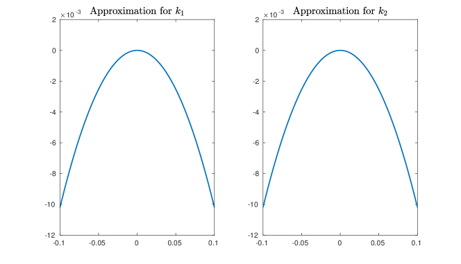
Figure 1: Approximation of the center manifold and residuals for Example 1 using kernels $k_{1}$ and $k_{2}$.

4.2 Example 2

We consider the $2$-dimensional system

$$\begin{split}\dot{x}&=f_{1}(x,y)=-xy\\ \dot{y}&=f_{2}(x,y)=x^{2}-y-2y^{2}.\end{split}$$ (12)

The training data is generated the same way as in Example 1. We again use the kernels $k_{1}$ and $k_{2}$. The greedy algorithm gives sets $X_{1}$ and $X_{2}$ of size $12$ and $6$, respectively. The evaluation of the approximations $s_{1}$ and $s_{2}$ over the neighborhood $[-0.1,0.1]$ can be seen on the left in Figure 2, while the respective pointwise residuals are plotted in the right part of Figure 2.

Figure 2: Approximation of the center manifold and residuals for Example 2 using kernels $k_{1}$ and $k_{2}$.

4.3 Example 3

We consider the $(2+1)$-dimensional system

$$\begin{split}\dot{x}&=f_{1}(x,y)=\begin{pmatrix}-x_{2}+x_{1}y\\ x_{1}+x_{2}y\end{pmatrix}\\ \dot{y}&=f_{2}(x,y)=-y-x_{1}^{2}-x_{2}^{2}+y^{2}.\end{split}$$ (13)

We generate the training data in a similar fashion as before. We again use the implicit Euler scheme with start time $t=0$, final time $T=1000$ and with time step $\Delta t=0.1$. The Euler method is performed for initial data $(x_{0},y_{0})\in\left\{\pm 0.8\right\}^{3}$ and the resulting trajectories are stored in $X$ and $Y$, where only data with $x\in[-0.1,0.1]^{2}$ was considered; this leads to $N^{\ast}=78796$ data pairs. We use the kernels $k_{1}(x,y)=(1+x^{T}y/2)^{4}$ and $k_{2}(x,y)=e^{-\|x-y\|_{2}^{2}/2}$, and the greedy-selected sets have the size $21$ (for $k_{1}$) and $25$ (for $k_{2}$), respectively. The approximations $s_{1}$,$s_{2}$ and their corresponding residuals $r_{1}$ and $r_{2}$ computed over the domain $[-0.1,0.1]^{2}$. The results can be seen in Figure 3.

Figure 3: Approximation of the center manifold and residuals for Example 3 using kernels $k_{1}$ and $k_{2}$.

We remark that in all the three experiments both kernels give comparable results in terms of error magnitude, and they both provide a good approximation of the manifold.

5 Conclusions

In this paper we introduced a novel algorithm to approximate the center manifold of a given ODE using a data-based surrogate.

This algorithm computes an approximation of the manifold from a set of numerical trajectories with different initial data. It is based on kernel methods, which allow the use of the scattered data generated by these simulations as training points. Moreover, an application-specific ansatz and cost function have been employed in order to enforce suitable properties on the surrogate.

Several numerical experiments suggested that the present method can reach a significant accuracy, and that it has the potential to be used as an effective model reduction technique. It seems promising to apply this approach to high dimensional systems as the approximation technique straightforwardly can be extended and is less prone to the curse of dimensionality than grid-based approximation techniques. An interesting extension would consist of determining the decomposition (2)–(3) in a data-based fashion by suitable processing of the trajectory data.

6 Acknowledgements

The first, third, and fourth authors would like to thank the German Research Foundation (DFG) for support within the Cluster of Excellence in Simulation Technology (EXC 310/2) at the University of Stuttgart.

References

- [1] J. Carr. Applications of centre manifold theory, volume 35 of Applied Mathematical Sciences. Springer-Verlag, New York-Berlin, 1981.
- [2] S. De Marchi, R. Schaback, and H. Wendland. Near-optimal data-independent point locations for radial basis function interpolation. Adv. Comput. Math., 23(3):317–330, 2005.
- [3] D. Henry. Geometric theory of semilinear parabolic equations, volume 840 of Lecture Notes in Mathematics. Springer-Verlag, Berlin-New York, 1981.
- [4] A. Kelley. The stable, center-stable, center, center-unstable, unstable manifolds. J. Differential Equations, 3:546–570, 1967.
- [5] C. A. Micchelli and M. Pontil. On learning vector-valued functions. Neural Comput., 17(1):177–204, 2005.
- [6] V. A. Pliss. A reduction principle in the theory of stability of motion. Izv. Akad. Nauk SSSR Ser. Mat., 28:1297–1324, 1964.
- [7] G. Santin and B. Haasdonk. Convergence rate of the data-independent P-greedy algorithm in kernel-based approximation. Dolomites Res. Notes Approx., 10:68–78, 2017.
- [8] A. N. Shoshitaishvili. Bifurcations of topological type of singular points of vector fields that depend on parameters. Funkcional. Anal. i Priložen., 6(2):97–98, 1972.
- [9] H. Wendland. Scattered Data Approximation, volume 17 of Cambridge Monographs on Applied and Computational Mathematics. Cambridge University Press, Cambridge, 2005.
- [10] D. Wittwar, G. Santin, and B. Haasdonk. Interpolation with uncoupled separable matrix-valued kernels. Dolomites Research Notes on Approximation, 2018. accepted.
- [11] D. Wittwar, G. Santin, and B. Haasdonk. Weighted regularized interpolation with matrix valued kernels. Technical report, University of Stuttgart, 2018. in preparation.