1 Introduction
Dynamic panels providing information on a large population of heterogeneous individuals such as households, firms, etc.
observed at regular time periods, are often described by simple autoregressive models with random parameters near
unity. One of the simplest models for individual evolution is
the random-coefficient AR(1) (RCAR(1)) process
X ( t ) = a X ( t − 1 ) + ε ( t ) , t ∈ ℤ , formulae-sequence 𝑋 𝑡 𝑎 𝑋 𝑡 1 𝜀 𝑡 𝑡 ℤ X(t)=aX(t-1)+\varepsilon(t),\quad t\in\mathbb{Z}, (1.1)
with standardized i.i.d. innovations { ε ( t ) , t ∈ ℤ } 𝜀 𝑡 𝑡
ℤ \{\varepsilon(t),t\in\mathbb{Z}\} a ∈ [ 0 , 1 ) 𝑎 0 1 a\in[0,1) { ε ( t ) , t ∈ ℤ } 𝜀 𝑡 𝑡
ℤ \{\varepsilon(t),t\in\mathbb{Z}\} [10 ] observed that
in the case when the distribution of a 𝑎 a 1.1 a ∈ [ 0 , 1 ) 𝑎 0 1 a\in[0,1)
ϕ ( x ) = ψ ( x ) ( 1 − x ) β − 1 , x ∈ [ 0 , 1 ) , formulae-sequence italic-ϕ 𝑥 𝜓 𝑥 superscript 1 𝑥 𝛽 1 𝑥 0 1 \phi(x)=\psi(x)(1-x)^{\beta-1},\quad x\in[0,1), (1.2)
where β > 0 𝛽 0 \beta>0 ψ ( x ) 𝜓 𝑥 \psi(x) x ∈ [ 0 , 1 ) 𝑥 0 1 x\in[0,1) lim x ↑ 1 ψ ( x ) = : ψ ( 1 ) > 0 \lim_{x\uparrow 1}\psi(x)=:\psi(1)>0 β > 1 𝛽 1 \beta>1 1.1 t − ( β − 1 ) superscript 𝑡 𝛽 1 t^{-(\beta-1)}
γ ( t ) := E X ( 0 ) X ( t ) = E a | t | 1 − a 2 ∼ ( ψ ( 1 ) / 2 ) Γ ( β − 1 ) t − ( β − 1 ) , t → ∞ , formulae-sequence assign 𝛾 𝑡 E 𝑋 0 𝑋 𝑡 E superscript 𝑎 𝑡 1 superscript 𝑎 2 similar-to 𝜓 1 2 Γ 𝛽 1 superscript 𝑡 𝛽 1 → 𝑡 \gamma(t):=\mathrm{E}X(0)X(t)=\mathrm{E}\frac{a^{|t|}}{1-a^{2}}\sim(\psi(1)/2)\Gamma(\beta-1)t^{-(\beta-1)},\qquad t\to\infty, (1.3)
implying
∑ t ∈ ℤ | Cov ( X ( 0 ) , X ( t ) ) | = ∞ subscript 𝑡 ℤ Cov 𝑋 0 𝑋 𝑡 \sum_{t\in\mathbb{Z}}|\operatorname{Cov}(X(0),X(t))|=\infty β ∈ ( 1 , 2 ] 𝛽 1 2 \beta\in(1,2] N 𝑁 N { X i ( t ) } , i = 1 , … , N formulae-sequence subscript 𝑋 𝑖 𝑡 𝑖
1 … 𝑁
\{X_{i}(t)\},i=1,\dots,N 1.1 N → ∞ → 𝑁 N\to\infty [9 ] , Zaffaroni [32 ] ,
Celov et al. [3 ] ,
Oppenheim and Viano [18 ] , Puplinskaitė and Surgailis [25 ] ,
Philippe et al. [19 ] and other works, see Leipus et al. [14 ] for review.
Statistical inference in the RCAR(1) model was discussed in several works.
Leipus et al. [13 ] , Celov et al. [4 ] discussed nonparametric estimation of the mixing density ϕ ( x ) italic-ϕ 𝑥 \phi(x) [29 ] and
Beran et al. [1 ] discussed parametric estimation of the mixing density.
In nonparametric context,
Leipus et al. [15 ] studied estimation of the empirical d.f. of a 𝑎 a N , n → ∞ → 𝑁 𝑛
N,n\to\infty [16 ] discussed estimation of
β 𝛽 \beta 1.2 N × n 𝑁 𝑛 N\times n N 𝑁 N { X i ( t ) , t = 1 , … , n } formulae-sequence subscript 𝑋 𝑖 𝑡 𝑡
1 … 𝑛
\{X_{i}(t),t=1,\dots,n\} n 𝑛 n i = 1 , … , N 𝑖 1 … 𝑁
i=1,\dots,N 1.1 1.2 [20 ] studied the asymptotic distribution of the sample mean
X ¯ N , n subscript ¯ 𝑋 𝑁 𝑛
\displaystyle\bar{X}_{N,n} := assign \displaystyle:= 1 N n ∑ i = 1 N ∑ t = 1 n X i ( t ) 1 𝑁 𝑛 superscript subscript 𝑖 1 𝑁 superscript subscript 𝑡 1 𝑛 subscript 𝑋 𝑖 𝑡 \displaystyle\frac{1}{Nn}\sum_{i=1}^{N}\sum_{t=1}^{n}X_{i}(t) (1.4)
as N , n → ∞ → 𝑁 𝑛
N,n\to\infty [20 ]
showed that for 0 < β < 2 0 𝛽 2 0<\beta<2 N / n β → ∞ → 𝑁 superscript 𝑛 𝛽 N/n^{\beta}\to\infty N / n β → 0 → 𝑁 superscript 𝑛 𝛽 0 N/n^{\beta}\to 0 X ¯ N , n subscript ¯ 𝑋 𝑁 𝑛
\bar{X}_{N,n} β 𝛽 \beta ( 0 , 2 ] 0 2 (0,2] [20 ] , under the
‘intermediate’ scaling N / n β → c ∈ ( 0 , ∞ ) → 𝑁 superscript 𝑛 𝛽 𝑐 0 N/n^{\beta}\to c\in(0,\infty) X ¯ N , n subscript ¯ 𝑋 𝑁 𝑛
\bar{X}_{N,n}
The present paper discusses asymptotic distribution of sample covariances (covariance estimates)
γ ^ N , n ( t , s ) subscript ^ 𝛾 𝑁 𝑛
𝑡 𝑠 \displaystyle\widehat{\gamma}_{N,n}(t,s) := assign \displaystyle:= 1 N n ∑ 1 ≤ i , i + s ≤ N ∑ 1 ≤ k , k + t ≤ n ( X i ( k ) − X ¯ N , n ) ( X i + s ( k + t ) − X ¯ N , n ) , ( t , s ) ∈ ℤ 2 , 1 𝑁 𝑛 subscript formulae-sequence 1 𝑖 𝑖 𝑠 𝑁 subscript formulae-sequence 1 𝑘 𝑘 𝑡 𝑛 subscript 𝑋 𝑖 𝑘 subscript ¯ 𝑋 𝑁 𝑛
subscript 𝑋 𝑖 𝑠 𝑘 𝑡 subscript ¯ 𝑋 𝑁 𝑛
𝑡 𝑠
superscript ℤ 2 \displaystyle\frac{1}{Nn}\sum_{1\leq i,i+s\leq N}\sum_{1\leq k,k+t\leq n}(X_{i}(k)-\bar{X}_{N,n})(X_{i+s}(k+t)-\bar{X}_{N,n}),\qquad(t,s)\in\mathbb{Z}^{2}, (1.5)
computed from a similar RCAR(1) panel { X i ( t ) , t = 1 , … , n , i = 1 , … , N } formulae-sequence subscript 𝑋 𝑖 𝑡 𝑡
1 … 𝑛 𝑖
1 … 𝑁
\{X_{i}(t),\,t=1,\dots,n,\,i=1,\dots,N\} [20 ] ,
as N , n 𝑁 𝑛
N,n ( t , s ) ∈ ℤ 2 𝑡 𝑠 superscript ℤ 2 (t,s)\in\mathbb{Z}^{2} ( t , s ) = ( 0 , 0 ) 𝑡 𝑠 0 0 (t,s)=(0,0) 1.5
γ ^ N , n ( 0 , 0 ) = 1 N n ∑ i = 1 N ∑ k = 1 n ( X i ( k ) − X ¯ N , n ) 2 . subscript ^ 𝛾 𝑁 𝑛
0 0 1 𝑁 𝑛 superscript subscript 𝑖 1 𝑁 superscript subscript 𝑘 1 𝑛 superscript subscript 𝑋 𝑖 𝑘 subscript ¯ 𝑋 𝑁 𝑛
2 \displaystyle{\widehat{\gamma}_{N,n}(0,0)}=\frac{1}{Nn}\sum_{i=1}^{N}\sum_{k=1}^{n}(X_{i}(k)-\bar{X}_{N,n})^{2}. (1.6)
The true covariance function γ ( t , s ) := E X i ( k ) X i + s ( k + t ) assign 𝛾 𝑡 𝑠 E subscript 𝑋 𝑖 𝑘 subscript 𝑋 𝑖 𝑠 𝑘 𝑡 \gamma(t,s):=\mathrm{E}X_{i}(k)X_{i+s}(k+t) 1.2 β > 1 𝛽 1 \beta>1
γ ( t , s ) = { γ ( t ) , s = 0 , 0 , s ≠ 0 , 𝛾 𝑡 𝑠 cases 𝛾 𝑡 𝑠 0 0 𝑠 0 \displaystyle\gamma(t,s)=\begin{cases}\gamma(t),&s=0,\\
0,&s\neq 0,\end{cases} (1.7)
where γ ( t ) 𝛾 𝑡 \gamma(t) 1.3 γ ( t ) 𝛾 𝑡 \gamma(t) { X ( t ) } 𝑋 𝑡 \{X(t)\} 1.1 1.7 N × n 𝑁 𝑛 N\times n N , n → ∞ → 𝑁 𝑛
N,n\to\infty 0 < β < 1 0 𝛽 1 0<\beta<1 γ ^ N , n ( t , s ) subscript ^ 𝛾 𝑁 𝑛
𝑡 𝑠 \widehat{\gamma}_{N,n}(t,s) N 𝑁 N n 𝑛 n s = 0 𝑠 0 s=0 s ≠ 0 𝑠 0 s\neq 0 s = 0 𝑠 0 s=0 s ≠ 0 𝑠 0 s\neq 0 1.5 X i ( k ) X i + s ( k + t ) subscript 𝑋 𝑖 𝑘 subscript 𝑋 𝑖 𝑠 𝑘 𝑡 X_{i}(k)X_{i+s}(k+t) X i subscript 𝑋 𝑖 X_{i} X i + s subscript 𝑋 𝑖 𝑠 X_{i+s} X i ( k ) subscript 𝑋 𝑖 𝑘 X_{i}(k) X i ( k + t ) subscript 𝑋 𝑖 𝑘 𝑡 X_{i}(k+t) [20 ] about the sample mean
in (1.4
Table 1: Limit distribution of sample covariances γ ^ N , n ( t , s ) subscript ^ 𝛾 𝑁 𝑛
𝑡 𝑠 \widehat{\gamma}_{N,n}(t,s) 1.5
Mutual increase rate of N , n 𝑁 𝑛
N,n
Parameter region
Limit distribution
N / n β → ∞ → 𝑁 superscript 𝑛 𝛽 N/n^{\beta}\to\infty 1 < β < 2 1 𝛽 2 1<\beta<2 Gaussian
0 < β < 1 0 𝛽 1 0<\beta<1 symmetric ( 2 β ) 2 𝛽 (2\beta)
N / n β → 0 → 𝑁 superscript 𝑛 𝛽 0 N/n^{\beta}\to 0 0 < β < 2 0 𝛽 2 0<\beta<2 symmetric β 𝛽 \beta
N / n β → c ∈ ( 0 , ∞ ) → 𝑁 superscript 𝑛 𝛽 𝑐 0 N/n^{\beta}\to c\in(0,\infty) 0 < β < 2 0 𝛽 2 0<\beta<2 ‘intermediate Poisson’
Arbitrary
β > 2 𝛽 2 \beta>2 Gaussian
Table 2: Limit distribution of the sample mean X ¯ N , n subscript ¯ 𝑋 𝑁 𝑛
\bar{X}_{N,n} 1.4
The rest of the paper is organized as follows. Section 2 presents some preliminary facts, including the
definition and properties of the intermediate processes appearing in Table 1.
Section 3 contains rigorous formulations and the proofs
of the asymptotic results for cross-sectional sample
covariances (1.5 s ≠ 0 𝑠 0 s\neq 0 γ ( t ) 𝛾 𝑡 \gamma(t) 1.3
2 Preliminaries
This section contains some preliminary facts which will be used in the following sections.
2.1. Double stochastic integrals and quadratic forms.
Let B i , i = 1 , 2 formulae-sequence subscript 𝐵 𝑖 𝑖
1 2 B_{i},i=1,2
I i ( f ) := ∫ ℝ f ( s ) d B i ( s ) , I i j ( g ) := ∫ ℝ 2 g ( s 1 , s 2 ) d B i ( s 1 ) d B j ( s 2 ) , i , j = 1 , 2 , formulae-sequence assign subscript 𝐼 𝑖 𝑓 subscript ℝ 𝑓 𝑠 differential-d subscript 𝐵 𝑖 𝑠 formulae-sequence assign subscript 𝐼 𝑖 𝑗 𝑔 subscript superscript ℝ 2 𝑔 subscript 𝑠 1 subscript 𝑠 2 differential-d subscript 𝐵 𝑖 subscript 𝑠 1 differential-d subscript 𝐵 𝑗 subscript 𝑠 2 𝑖
𝑗 1 2
I_{i}(f):=\int_{\mathbb{R}}f(s)\mathrm{d}B_{i}(s),\qquad I_{ij}(g):=\int_{\mathbb{R}^{2}}g(s_{1},s_{2})\mathrm{d}B_{i}(s_{1})\mathrm{d}B_{j}(s_{2}),\quad i,j=1,2, (2.1)
denote Itô-Wiener stochastic integrals (single and double)
w.r.t. B i , B j subscript 𝐵 𝑖 subscript 𝐵 𝑗
B_{i},B_{j} 2.1 f ∈ L 2 ( ℝ ) , g ∈ L 2 ( ℝ 2 ) formulae-sequence 𝑓 superscript 𝐿 2 ℝ 𝑔 superscript 𝐿 2 superscript ℝ 2 f\in L^{2}(\mathbb{R}),g\in L^{2}(\mathbb{R}^{2}) E I i ( f ) = E I i j ( g ) = 0 E subscript 𝐼 𝑖 𝑓 E subscript 𝐼 𝑖 𝑗 𝑔 0 \mathrm{E}I_{i}(f)=\mathrm{E}I_{ij}(g)=0
E I i ( f ) I i ′ ( f ′ ) E subscript 𝐼 𝑖 𝑓 subscript 𝐼 superscript 𝑖 ′ superscript 𝑓 ′ \displaystyle\mathrm{E}I_{i}(f)I_{i^{\prime}}(f^{\prime}) = \displaystyle= { 0 , i ≠ i ′ , ⟨ f , f ′ ⟩ , i = i ′ , f , f ′ ∈ L 2 ( ℝ ) , cases 0 𝑖 superscript 𝑖 ′ 𝑓 superscript 𝑓 ′
𝑖 superscript 𝑖 ′ 𝑓 superscript 𝑓 ′
superscript 𝐿 2 ℝ \displaystyle\begin{cases}0,&i\neq i^{\prime},\\
\langle f,f^{\prime}\rangle,&i=i^{\prime},\end{cases}\quad f,f^{\prime}\in L^{2}(\mathbb{R}), (2.2)
E I i ( f ) I i ′ j ′ ( g ) E subscript 𝐼 𝑖 𝑓 subscript 𝐼 superscript 𝑖 ′ superscript 𝑗 ′ 𝑔 \displaystyle\mathrm{E}I_{i}(f)I_{i^{\prime}j^{\prime}}(g) = \displaystyle= 0 , ∀ i , i ′ , j ′ , f ∈ L 2 ( ℝ ) , g ∈ L 2 ( ℝ 2 ) , formulae-sequence 0 for-all 𝑖 superscript 𝑖 ′ superscript 𝑗 ′ 𝑓
superscript 𝐿 2 ℝ 𝑔 superscript 𝐿 2 superscript ℝ 2 \displaystyle 0,\hskip 42.67912pt\forall i,i^{\prime},j^{\prime},\quad f\in L^{2}(\mathbb{R}),g\in L^{2}(\mathbb{R}^{2}),
E I i j ( g ) I i ′ j ′ ( g ′ ) E subscript 𝐼 𝑖 𝑗 𝑔 subscript 𝐼 superscript 𝑖 ′ superscript 𝑗 ′ superscript 𝑔 ′ \displaystyle\mathrm{E}I_{ij}(g)I_{i^{\prime}j^{\prime}}(g^{\prime}) = \displaystyle= { 0 , ( i , j ) ∉ { ( i ′ , j ′ ) , ( j ′ , i ′ ) } , ⟨ g , g ′ ⟩ , ( i , j ) ∈ { ( i ′ , j ′ ) , ( j ′ , i ′ ) } , i ≠ j , 2 ⟨ g , sym g ′ ⟩ , i = i ′ = j = j ′ , g , g ′ ∈ L 2 ( ℝ 2 ) , cases 0 𝑖 𝑗 superscript 𝑖 ′ superscript 𝑗 ′ superscript 𝑗 ′ superscript 𝑖 ′ 𝑔 superscript 𝑔 ′
formulae-sequence 𝑖 𝑗 superscript 𝑖 ′ superscript 𝑗 ′ superscript 𝑗 ′ superscript 𝑖 ′ 𝑖 𝑗 2 𝑔 sym superscript 𝑔 ′
𝑖 superscript 𝑖 ′ 𝑗 superscript 𝑗 ′ 𝑔 superscript 𝑔 ′
superscript 𝐿 2 superscript ℝ 2 \displaystyle\begin{cases}0,&(i,j)\notin\{(i^{\prime},j^{\prime}),(j^{\prime},i^{\prime})\},\\
\langle g,g^{\prime}\rangle,&(i,j)\in\{(i^{\prime},j^{\prime}),(j^{\prime},i^{\prime})\},\ i\neq j,\\
2\langle g,{\rm sym}g^{\prime}\rangle,&i=i^{\prime}=j=j^{\prime},\end{cases}\qquad g,g^{\prime}\in L^{2}(\mathbb{R}^{2}),
where ⟨ f , f ′ ⟩ = ∫ ℝ f ( s ) f ′ ( s ) d s 𝑓 superscript 𝑓 ′
subscript ℝ 𝑓 𝑠 superscript 𝑓 ′ 𝑠 differential-d 𝑠 \langle f,f^{\prime}\rangle=\int_{\mathbb{R}}f(s)f^{\prime}(s){\rm d}s ( ‖ f ‖ := ⟨ f , f ⟩ ) , ⟨ g , g ′ ⟩ = ∫ ℝ 2 g ( s 1 , s 2 ) g ′ ( s 1 , s 2 ) d s 1 d s 2 assign norm 𝑓 𝑓 𝑓
𝑔 superscript 𝑔 ′
subscript superscript ℝ 2 𝑔 subscript 𝑠 1 subscript 𝑠 2 superscript 𝑔 ′ subscript 𝑠 1 subscript 𝑠 2 differential-d subscript 𝑠 1 differential-d subscript 𝑠 2 (\|f\|:=\sqrt{\langle f,f\rangle}),\langle g,g^{\prime}\rangle=\int_{\mathbb{R}^{2}}g(s_{1},s_{2})g^{\prime}(s_{1},s_{2})\mathrm{d}s_{1}\mathrm{d}s_{2} ( ‖ g ‖ := ⟨ g , g ⟩ ) assign norm 𝑔 𝑔 𝑔
(\|g\|:=\sqrt{\langle g,g\rangle}) L 2 ( ℝ ) superscript 𝐿 2 ℝ L^{2}(\mathbb{R}) L 2 ( ℝ 2 ) superscript 𝐿 2 superscript ℝ 2 L^{2}(\mathbb{R}^{2}) sym sym {\rm sym} [7 ] , sec. 11.5, 14.3). Note that for g ( s 1 , s 2 ) = f 1 ( s 1 ) f 2 ( s 2 ) , f i ∈ L 2 ( ℝ ) , i = 1 , 2 formulae-sequence 𝑔 subscript 𝑠 1 subscript 𝑠 2 subscript 𝑓 1 subscript 𝑠 1 subscript 𝑓 2 subscript 𝑠 2 formulae-sequence subscript 𝑓 𝑖 superscript 𝐿 2 ℝ 𝑖 1 2
g(s_{1},s_{2})=f_{1}(s_{1})f_{2}(s_{2}),f_{i}\in L^{2}(\mathbb{R}),i=1,2 I i i ( g ) = I i ( f 1 ) I i ( f 2 ) − ⟨ f 1 , f 2 ⟩ , I 12 ( g ) = I 1 ( f 1 ) I 2 ( f 2 ) , formulae-sequence subscript 𝐼 𝑖 𝑖 𝑔 subscript 𝐼 𝑖 subscript 𝑓 1 subscript 𝐼 𝑖 subscript 𝑓 2 subscript 𝑓 1 subscript 𝑓 2
subscript 𝐼 12 𝑔 subscript 𝐼 1 subscript 𝑓 1 subscript 𝐼 2 subscript 𝑓 2 I_{ii}(g)=I_{i}(f_{1})I_{i}(f_{2})-\langle f_{1},f_{2}\rangle,\ I_{12}(g)=I_{1}(f_{1})I_{2}(f_{2}), I 12 ( g ) = d ‖ f 1 ‖ ‖ f 2 ‖ Z 1 Z 2 , subscript d subscript 𝐼 12 𝑔 norm subscript 𝑓 1 norm subscript 𝑓 2 subscript 𝑍 1 subscript 𝑍 2 I_{12}(g)=_{\rm d}\|f_{1}\|\|f_{2}\|Z_{1}Z_{2}, Z i ∼ N ( 0 , 1 ) , i = 1 , 2 formulae-sequence similar-to subscript 𝑍 𝑖 𝑁 0 1 𝑖 1 2
Z_{i}\sim N(0,1),i=1,2
Let { ε i ( s ) , s ∈ ℤ } , i = 1 , 2 formulae-sequence subscript 𝜀 𝑖 𝑠 𝑠
ℤ 𝑖
1 2 \{\varepsilon_{i}(s),s\in\mathbb{Z}\},i=1,2 E ε i ( s ) = 0 E subscript 𝜀 𝑖 𝑠 0 \mathrm{E}\varepsilon_{i}(s)=0 E ε i ( s ) ε i ′ ( s ′ ) = 1 E subscript 𝜀 𝑖 𝑠 subscript 𝜀 superscript 𝑖 ′ superscript 𝑠 ′ 1 \mathrm{E}\varepsilon_{i}(s)\varepsilon_{i^{\prime}}(s^{\prime})=1 ( i , s ) = ( i ′ , s ′ ) 𝑖 𝑠 superscript 𝑖 ′ superscript 𝑠 ′ (i,s)=(i^{\prime},s^{\prime}) E ε i ( s ) ε i ′ ( s ′ ) = 0 E subscript 𝜀 𝑖 𝑠 subscript 𝜀 superscript 𝑖 ′ superscript 𝑠 ′ 0 \mathrm{E}\varepsilon_{i}(s)\varepsilon_{i^{\prime}}(s^{\prime})=0 ( i , s ) ≠ ( i ′ , s ′ ) 𝑖 𝑠 superscript 𝑖 ′ superscript 𝑠 ′ (i,s)\neq(i^{\prime},s^{\prime}) i , i ′ = 1 , 2 formulae-sequence 𝑖 superscript 𝑖 ′
1 2 i,i^{\prime}=1,2 s , s ′ ∈ ℤ 𝑠 superscript 𝑠 ′
ℤ s,s^{\prime}\in\mathbb{Z}
Q i j ( h ) = ∑ s 1 , s 2 ∈ ℤ h ( s 1 , s 2 ) [ ε i ( s 1 ) ε j ( s 2 ) − E ε i ( s 1 ) ε j ( s 2 ) ] , i , j = 1 , 2 , formulae-sequence subscript 𝑄 𝑖 𝑗 ℎ subscript subscript 𝑠 1 subscript 𝑠 2
ℤ ℎ subscript 𝑠 1 subscript 𝑠 2 delimited-[] subscript 𝜀 𝑖 subscript 𝑠 1 subscript 𝜀 𝑗 subscript 𝑠 2 E subscript 𝜀 𝑖 subscript 𝑠 1 subscript 𝜀 𝑗 subscript 𝑠 2 𝑖
𝑗 1 2
Q_{ij}(h)=\sum_{s_{1},s_{2}\in\mathbb{Z}}h(s_{1},s_{2})[\varepsilon_{i}(s_{1})\varepsilon_{j}(s_{2})-\mathrm{E}\varepsilon_{i}(s_{1})\varepsilon_{j}(s_{2})],\qquad i,j=1,2, (2.3)
where h ∈ L 2 ( ℤ 2 ) ℎ superscript 𝐿 2 superscript ℤ 2 h\in L^{2}(\mathbb{Z}^{2}) i = j 𝑖 𝑗 i=j E ε i 4 ( 0 ) < ∞ E subscript superscript 𝜀 4 𝑖 0 \mathrm{E}\varepsilon^{4}_{i}(0)<\infty 2.3 L 2 superscript 𝐿 2 L^{2}
var ( Q i j ( h ) ) ≤ ( 1 + E ε i 4 ( 0 ) δ i j ) ∑ s 1 , s 2 ∈ ℤ h 2 ( s 1 , s 2 ) , var subscript 𝑄 𝑖 𝑗 ℎ 1 E subscript superscript 𝜀 4 𝑖 0 subscript 𝛿 𝑖 𝑗 subscript subscript 𝑠 1 subscript 𝑠 2
ℤ superscript ℎ 2 subscript 𝑠 1 subscript 𝑠 2 {\rm var}(Q_{ij}(h))\leq(1+\mathrm{E}\varepsilon^{4}_{i}(0)\delta_{ij})\sum_{s_{1},s_{2}\in\mathbb{Z}}h^{2}(s_{1},s_{2}), (2.4)
see ([7 ] , (4.5.4)). With any h ∈ L 2 ( ℤ 2 ) ℎ superscript 𝐿 2 superscript ℤ 2 h\in L^{2}(\mathbb{Z}^{2}) α 1 , α 2 > 0 subscript 𝛼 1 subscript 𝛼 2
0 \alpha_{1},\alpha_{2}>0 L 2 ( ℝ 2 ) superscript 𝐿 2 superscript ℝ 2 L^{2}(\mathbb{R}^{2})
h ~ ( α 1 , α 2 ) ( s 1 , s 2 ) := ( α 1 α 2 ) 1 / 2 h ( ⌊ α 1 s 1 ⌋ , ⌊ α 2 s 2 ⌋ ) , ( s 1 , s 2 ) ∈ ℝ 2 , formulae-sequence assign superscript ~ ℎ subscript 𝛼 1 subscript 𝛼 2 subscript 𝑠 1 subscript 𝑠 2 superscript subscript 𝛼 1 subscript 𝛼 2 1 2 ℎ subscript 𝛼 1 subscript 𝑠 1 subscript 𝛼 2 subscript 𝑠 2 subscript 𝑠 1 subscript 𝑠 2 superscript ℝ 2 \widetilde{h}^{(\alpha_{1},\alpha_{2})}(s_{1},s_{2}):=(\alpha_{1}\alpha_{2})^{1/2}h(\lfloor\alpha_{1}s_{1}\rfloor,\lfloor\alpha_{2}s_{2}\rfloor),\qquad(s_{1},s_{2})\in\mathbb{R}^{2}, (2.5)
with ‖ h ~ ( α 1 , α 2 ) ‖ 2 = ∑ s 1 , s 2 ∈ ℤ h 2 ( s 1 , s 2 ) superscript norm superscript ~ ℎ subscript 𝛼 1 subscript 𝛼 2 2 subscript subscript 𝑠 1 subscript 𝑠 2
ℤ superscript ℎ 2 subscript 𝑠 1 subscript 𝑠 2 \|\widetilde{h}^{(\alpha_{1},\alpha_{2})}\|^{2}=\sum_{s_{1},s_{2}\in\mathbb{Z}}h^{2}(s_{1},s_{2}) 2.3 2.1
Proposition 2.1 .
([7 ] , Proposition 11.5.5) Let i , j = 1 , 2 formulae-sequence 𝑖 𝑗
1 2 i,j=1,2 Q i j ( h α 1 , α 2 ) , α 1 , α 2 > 0 subscript 𝑄 𝑖 𝑗 subscript ℎ subscript 𝛼 1 subscript 𝛼 2
subscript 𝛼 1 subscript 𝛼 2
0 Q_{ij}(h_{\alpha_{1},\alpha_{2}}),\alpha_{1},\alpha_{2}>0 2.3 h α 1 , α 2 ∈ L 2 ( ℤ 2 ) subscript ℎ subscript 𝛼 1 subscript 𝛼 2
superscript 𝐿 2 superscript ℤ 2 h_{\alpha_{1},\alpha_{2}}\in L^{2}(\mathbb{Z}^{2}) i = j 𝑖 𝑗 i=j E ε i 4 ( 0 ) < ∞ E subscript superscript 𝜀 4 𝑖 0 \mathrm{E}\varepsilon^{4}_{i}(0)<\infty g ∈ L 2 ( ℝ 2 ) 𝑔 superscript 𝐿 2 superscript ℝ 2 g\in L^{2}(\mathbb{R}^{2})
lim α 1 , α 2 → ∞ ‖ h ~ α 1 , α 2 ( α 1 , α 2 ) − g ‖ = 0 . subscript → subscript 𝛼 1 subscript 𝛼 2
norm subscript superscript ~ ℎ subscript 𝛼 1 subscript 𝛼 2 subscript 𝛼 1 subscript 𝛼 2
𝑔 0 \lim_{\alpha_{1},\alpha_{2}\to\infty}\|\widetilde{h}^{(\alpha_{1},\alpha_{2})}_{\alpha_{1},\alpha_{2}}-g\|=0. (2.6)
Then Q i j ( h α 1 , α 2 ) → d I i j ( g ) ( α 1 , α 2 → ∞ ) subscript → d subscript 𝑄 𝑖 𝑗 subscript ℎ subscript 𝛼 1 subscript 𝛼 2
subscript 𝐼 𝑖 𝑗 𝑔 → subscript 𝛼 1 subscript 𝛼 2
Q_{ij}(h_{\alpha_{1},\alpha_{2}})\to_{\rm d}I_{ij}(g)\ (\alpha_{1},\alpha_{2}\to\infty) I i j ( g ) subscript 𝐼 𝑖 𝑗 𝑔 I_{ij}(g) 2.1
2.2. The ‘cross-sectional’ intermediate process. Let d ℳ β ≡ ℳ β ( d x 1 , d x 2 , d B 1 , d B 2 ) d subscript ℳ 𝛽 subscript ℳ 𝛽 d subscript 𝑥 1 d subscript 𝑥 2 d subscript 𝐵 1 d subscript 𝐵 2 \mathrm{d}{\cal M}_{\beta}\equiv{\cal M}_{\beta}(\mathrm{d}x_{1},\mathrm{d}x_{2},\mathrm{d}B_{1},\mathrm{d}B_{2}) ( ℝ + × C ( ℝ ) ) 2 superscript subscript ℝ 𝐶 ℝ 2 (\mathbb{R}_{+}\times C(\mathbb{R}))^{2}
d μ β ≡ μ β ( d x 1 , d x 2 , d B 1 , d B 2 ) := ψ ( 1 ) 2 ( x 1 x 2 ) β − 1 d x 1 d x 2 P B ( d B 1 ) P B ( d B 2 ) , d subscript 𝜇 𝛽 subscript 𝜇 𝛽 d subscript 𝑥 1 d subscript 𝑥 2 d subscript 𝐵 1 d subscript 𝐵 2 assign 𝜓 superscript 1 2 superscript subscript 𝑥 1 subscript 𝑥 2 𝛽 1 d subscript 𝑥 1 d subscript 𝑥 2 subscript 𝑃 𝐵 d subscript 𝐵 1 subscript 𝑃 𝐵 d subscript 𝐵 2 \mathrm{d}\mu_{\beta}\equiv\mu_{\beta}(\mathrm{d}x_{1},\mathrm{d}x_{2},\mathrm{d}B_{1},\mathrm{d}B_{2}):=\psi(1)^{2}(x_{1}x_{2})^{\beta-1}\mathrm{d}x_{1}\mathrm{d}x_{2}P_{B}(\mathrm{d}B_{1})P_{B}(\mathrm{d}B_{2}), (2.7)
where β > 0 𝛽 0 \beta>0 P B subscript 𝑃 𝐵 P_{B} C ( ℝ ) 𝐶 ℝ C(\mathbb{R}) d ℳ ~ β := d ℳ β − d μ β assign d subscript ~ ℳ 𝛽 d subscript ℳ 𝛽 d subscript 𝜇 𝛽 \mathrm{d}\widetilde{\cal M}_{\beta}:=\mathrm{d}{\cal M}_{\beta}-\mathrm{d}\mu_{\beta}
∫ ℝ + 2 min { 1 , 1 x 1 x 2 ( x 1 + x 2 ) } ( x 1 x 2 ) β − 1 d x 1 d x 2 < ∞ , ∀ 0 < β < 3 / 2 , formulae-sequence subscript subscript superscript ℝ 2 1 1 subscript 𝑥 1 subscript 𝑥 2 subscript 𝑥 1 subscript 𝑥 2 superscript subscript 𝑥 1 subscript 𝑥 2 𝛽 1 differential-d subscript 𝑥 1 differential-d subscript 𝑥 2 for-all 0 𝛽 3 2 \displaystyle\int_{\mathbb{R}^{2}_{+}}\min\big{\{}1,\frac{1}{x_{1}x_{2}(x_{1}+x_{2})}\big{\}}(x_{1}x_{2})^{\beta-1}\mathrm{d}x_{1}\mathrm{d}x_{2}<\infty,\qquad\forall\,0<\beta<3/2, (2.8)
∫ ℝ + 2 min { 1 , 1 x 1 + x 2 } ( x 1 x 2 ) β − 2 d x 1 d x 2 < ∞ , ∀ 1 < β < 3 / 2 , formulae-sequence subscript subscript superscript ℝ 2 1 1 subscript 𝑥 1 subscript 𝑥 2 superscript subscript 𝑥 1 subscript 𝑥 2 𝛽 2 differential-d subscript 𝑥 1 differential-d subscript 𝑥 2 for-all 1 𝛽 3 2 \displaystyle\int_{\mathbb{R}^{2}_{+}}\min\big{\{}1,\frac{1}{x_{1}+x_{2}}\big{\}}(x_{1}x_{2})^{\beta-2}\mathrm{d}x_{1}\mathrm{d}x_{2}\ <\ \infty,\qquad\forall\,1<\beta<3/2, (2.9)
see Appendix. Let
𝒴 i ( u ; x ) = ∫ − ∞ u e − x ( u − s ) d B i ( s ) , u ∈ ℝ , x > 0 , formulae-sequence subscript 𝒴 𝑖 𝑢 𝑥
superscript subscript 𝑢 superscript e 𝑥 𝑢 𝑠 differential-d subscript 𝐵 𝑖 𝑠 formulae-sequence 𝑢 ℝ 𝑥 0 {\cal Y}_{i}(u;x)=\int_{-\infty}^{u}\mathrm{e}^{-x(u-s)}\mathrm{d}B_{i}(s),\qquad u\in\mathbb{R},\ x>0, (2.10)
be a family of stationary Ornstein-Uhlenbeck (O-U) processes subordinated to B i = { B i ( s ) , s ∈ ℝ } subscript 𝐵 𝑖 subscript 𝐵 𝑖 𝑠 𝑠
ℝ B_{i}=\{B_{i}(s),s\in\mathbb{R}\} B i , i = 1 , 2 formulae-sequence subscript 𝐵 𝑖 𝑖
1 2 B_{i},i=1,2
z ( τ ; x 1 , x 2 ) 𝑧 𝜏 subscript 𝑥 1 subscript 𝑥 2
\displaystyle z(\tau;x_{1},x_{2}) := assign \displaystyle:= ∫ 0 τ ∏ i = 1 2 𝒴 i ( u ; x i ) d u , τ ≥ 0 , superscript subscript 0 𝜏 superscript subscript product 𝑖 1 2 subscript 𝒴 𝑖 𝑢 subscript 𝑥 𝑖
d 𝑢 𝜏
0 \displaystyle\int_{0}^{\tau}\prod_{i=1}^{2}{\cal Y}_{i}(u;x_{i})\mathrm{d}u,\qquad\tau\geq 0, (2.11)
be a family of
integrated products of independent O-U processes indexed by x 1 , x 2 > 0 subscript 𝑥 1 subscript 𝑥 2
0 x_{1},x_{2}>0 2.11
z ( τ ; x 1 , x 2 ) 𝑧 𝜏 subscript 𝑥 1 subscript 𝑥 2
\displaystyle z(\tau;x_{1},x_{2}) = \displaystyle= ∫ ℝ 2 { ∫ 0 τ ∏ i = 1 2 e − x i ( u − s i ) 𝟏 ( u > s i ) d u } d B 1 ( s 1 ) d B 2 ( s 2 ) subscript superscript ℝ 2 superscript subscript 0 𝜏 superscript subscript product 𝑖 1 2 superscript e subscript 𝑥 𝑖 𝑢 subscript 𝑠 𝑖 1 𝑢 subscript 𝑠 𝑖 d 𝑢 differential-d subscript 𝐵 1 subscript 𝑠 1 differential-d subscript 𝐵 2 subscript 𝑠 2 \displaystyle\int_{\mathbb{R}^{2}}\big{\{}\int_{0}^{\tau}\prod_{i=1}^{2}\mathrm{e}^{-x_{i}(u-s_{i})}{\bf 1}(u>s_{i})\mathrm{d}u\big{\}}\mathrm{d}B_{1}(s_{1})\mathrm{d}B_{2}(s_{2}) (2.12)
as the double Itô-Wiener integral in (2.1 𝒵 β subscript 𝒵 𝛽 {\cal Z}_{\beta} ℳ β subscript ℳ 𝛽 {\cal M}_{\beta}
𝒵 β ( τ ) subscript 𝒵 𝛽 𝜏 \displaystyle{\cal Z}_{\beta}(\tau) := assign \displaystyle:= ∫ ℒ 1 z ( τ ; x 1 , x 2 ) d ℳ β + ∫ ℒ 1 c z ( τ ; x 1 , x 2 ) d ℳ ~ β , subscript subscript ℒ 1 𝑧 𝜏 subscript 𝑥 1 subscript 𝑥 2
differential-d subscript ℳ 𝛽 subscript subscript superscript ℒ 𝑐 1 𝑧 𝜏 subscript 𝑥 1 subscript 𝑥 2
differential-d subscript ~ ℳ 𝛽 \displaystyle\int_{{\cal L}_{1}}z(\tau;x_{1},x_{2})\mathrm{d}{\cal M}_{\beta}+\int_{{\cal L}^{c}_{1}}z(\tau;x_{1},x_{2})\mathrm{d}\widetilde{\cal M}_{\beta}, (2.13)
where
ℒ 1 := { ( x 1 , x 2 , B 1 , B 2 ) ∈ ( ℝ + × C ( ℝ ) ) 2 : x 1 x 2 ( x 1 + x 2 ) ≤ 1 } , ℒ 1 c := ( ℝ + × C ( ℝ ) ) 2 ∖ ℒ 1 formulae-sequence assign subscript ℒ 1 conditional-set subscript 𝑥 1 subscript 𝑥 2 subscript 𝐵 1 subscript 𝐵 2 superscript subscript ℝ 𝐶 ℝ 2 subscript 𝑥 1 subscript 𝑥 2 subscript 𝑥 1 subscript 𝑥 2 1 assign subscript superscript ℒ 𝑐 1 superscript subscript ℝ 𝐶 ℝ 2 subscript ℒ 1 {\cal L}_{1}:=\{(x_{1},x_{2},B_{1},B_{2})\in(\mathbb{R}_{+}\times C(\mathbb{R}))^{2}:x_{1}x_{2}(x_{1}+x_{2})\leq 1\},\qquad{\cal L}^{c}_{1}:=(\mathbb{R}_{+}\times C(\mathbb{R}))^{2}\setminus{\cal L}_{1} (2.14)
and μ β ( ℒ 1 ) < ∞ subscript 𝜇 𝛽 subscript ℒ 1 \mu_{\beta}({\cal L}_{1})<\infty 1 / 2 < β < 3 / 2 1 2 𝛽 3 2 1/2<\beta<3/2 2.13
𝒵 β ( τ ) subscript 𝒵 𝛽 𝜏 \displaystyle{\cal Z}_{\beta}(\tau) = \displaystyle= ∫ ( ℝ + × C ( ℝ ) ) 2 z ( τ ; x 1 , x 2 ) d ℳ ~ β . subscript superscript subscript ℝ 𝐶 ℝ 2 𝑧 𝜏 subscript 𝑥 1 subscript 𝑥 2
differential-d subscript ~ ℳ 𝛽 \displaystyle\int_{(\mathbb{R}_{+}\times C(\mathbb{R}))^{2}}z(\tau;x_{1},x_{2})\mathrm{d}\widetilde{\cal M}_{\beta}. (2.15)
These and other properties of 𝒵 β subscript 𝒵 𝛽 {\cal Z}_{\beta} [28 ] and
[20 ] for general properties of stochastic integrals w.r.t. Poisson random measure.
Proposition 2.2 .
(i) The process 𝒵 β subscript 𝒵 𝛽 {\cal Z}_{\beta} 2.13 0 < β < 3 / 2 0 𝛽 3 2 0<\beta<3/2
E exp { i ∑ j = 1 m θ j 𝒵 β ( τ j ) } E i superscript subscript 𝑗 1 𝑚 subscript 𝜃 𝑗 subscript 𝒵 𝛽 subscript 𝜏 𝑗 \displaystyle\mathrm{E}\exp\big{\{}\mathrm{i}\sum_{j=1}^{m}\theta_{j}{\cal Z}_{\beta}(\tau_{j})\big{\}} = \displaystyle= exp { ∫ ( ℝ + × C ( ℝ ) ) 2 ( e i ∑ j = 1 m θ j z ( τ j ; x 1 , x 2 ) − 1 ) d μ β } , subscript superscript subscript ℝ 𝐶 ℝ 2 superscript e i superscript subscript 𝑗 1 𝑚 subscript 𝜃 𝑗 𝑧 subscript 𝜏 𝑗 subscript 𝑥 1 subscript 𝑥 2
1 differential-d subscript 𝜇 𝛽 \displaystyle\exp\Big{\{}\int_{(\mathbb{R}_{+}\times C(\mathbb{R}))^{2}}\big{(}\mathrm{e}^{\mathrm{i}\sum_{j=1}^{m}\theta_{j}z(\tau_{j};x_{1},x_{2})}-1\big{)}\mathrm{d}\mu_{\beta}\Big{\}}, (2.16)
where θ j ∈ ℝ , τ j ≥ 0 , j = 1 , … , m , m ∈ ℕ formulae-sequence subscript 𝜃 𝑗 ℝ formulae-sequence subscript 𝜏 𝑗 0 formulae-sequence 𝑗 1 … 𝑚
𝑚 ℕ \theta_{j}\in\mathbb{R},\tau_{j}\geq 0,j=1,\dots,m,\,m\in\mathbb{N} 𝒵 β subscript 𝒵 𝛽 {\cal Z}_{\beta} { 𝒵 β ( τ ) , τ ≥ 0 } = fdd { − 𝒵 β ( τ ) , τ ≥ 0 } . subscript fdd subscript 𝒵 𝛽 𝜏 𝜏
0 subscript 𝒵 𝛽 𝜏 𝜏
0 \{{\cal Z}_{\beta}(\tau),\tau\geq 0\}=_{\rm fdd}\{-{\cal Z}_{\beta}(\tau),\tau\geq 0\}.
(ii) E | 𝒵 β ( τ ) | p < ∞ E superscript subscript 𝒵 𝛽 𝜏 𝑝 \mathrm{E}|{\cal Z}_{\beta}(\tau)|^{p}<\infty for p < 2 β 𝑝 2 𝛽 p<2\beta and E 𝒵 β ( τ ) = 0 E subscript 𝒵 𝛽 𝜏 0 \mathrm{E}{\cal Z}_{\beta}(\tau)=0
for 1 / 2 < β < 3 / 2 1 2 𝛽 3 2 1/2<\beta<3/2 .
(iii) For 1 / 2 < β < 3 / 2 1 2 𝛽 3 2 1/2<\beta<3/2 , 𝒵 β subscript 𝒵 𝛽 {\cal Z}_{\beta} can be defined as in ( 2.15 ). Moreover, if 1 < β < 3 / 2 1 𝛽 3 2 1<\beta<3/2 , then
E 𝒵 β 2 ( τ ) < ∞ E subscript superscript 𝒵 2 𝛽 𝜏 \mathrm{E}{\cal Z}^{2}_{\beta}(\tau)<\infty and
E 𝒵 β ( τ 1 ) 𝒵 β ( τ 2 ) = ( σ ∞ 2 / 2 ) ( τ 1 2 ( 2 − β ) + τ 2 2 ( 2 − β ) − | τ 2 − τ 1 | 2 ( 2 − β ) ) , τ 1 , τ 2 ≥ 0 , formulae-sequence E subscript 𝒵 𝛽 subscript 𝜏 1 subscript 𝒵 𝛽 subscript 𝜏 2 subscript superscript 𝜎 2 2 superscript subscript 𝜏 1 2 2 𝛽 superscript subscript 𝜏 2 2 2 𝛽 superscript subscript 𝜏 2 subscript 𝜏 1 2 2 𝛽 subscript 𝜏 1
subscript 𝜏 2 0 \mathrm{E}{\cal Z}_{\beta}(\tau_{1}){\cal Z}_{\beta}(\tau_{2})=(\sigma^{2}_{\infty}/2)\big{(}\tau_{1}^{2(2-\beta)}+\tau_{2}^{2(2-\beta)}-|\tau_{2}-\tau_{1}|^{2(2-\beta)}\big{)},\quad\tau_{1},\tau_{2}\geq 0, (2.17)
where σ ∞ 2 := ψ ( 1 ) 2 Γ ( β − 1 ) 2 / ( 4 ( 2 − β ) ( 3 − 2 β ) ) assign subscript superscript 𝜎 2 𝜓 superscript 1 2 Γ superscript 𝛽 1 2 4 2 𝛽 3 2 𝛽 \sigma^{2}_{\infty}:=\psi(1)^{2}\Gamma(\beta-1)^{2}/(4(2-\beta)(3-2\beta)) .
(iv) For 1 / 2 < β < 3 / 2 1 2 𝛽 3 2 1/2<\beta<3/2 , the process 𝒵 β subscript 𝒵 𝛽 {\cal Z}_{\beta} has a.s. continuous trajectories.
(v) (Asymptotic self-similarity) As b → 0 → 𝑏 0 b\to 0 ,
b β − 2 𝒵 β ( b τ ) superscript 𝑏 𝛽 2 subscript 𝒵 𝛽 𝑏 𝜏 \displaystyle b^{\beta-2}{\cal Z}_{\beta}(b\tau) → fdd σ ∞ B 2 − β ( τ ) , if 1 < β < 3 / 2 , formulae-sequence subscript → fdd absent subscript 𝜎 subscript 𝐵 2 𝛽 𝜏 if 1 𝛽 3 2 \displaystyle\to_{\rm fdd}\sigma_{\infty}B_{2-\beta}(\tau),\qquad\text{if }1<\beta<3/2, (2.18)
b − 1 ( log b − 1 ) − 1 / ( 2 β ) 𝒵 β ( b τ ) superscript 𝑏 1 superscript superscript 𝑏 1 1 2 𝛽 subscript 𝒵 𝛽 𝑏 𝜏 \displaystyle b^{-1}(\log b^{-1})^{-1/(2\beta)}{\cal Z}_{\beta}(b\tau) → fdd τ V 2 β , if 0 < β < 1 , formulae-sequence subscript → fdd absent 𝜏 subscript 𝑉 2 𝛽 if 0 𝛽 1 \displaystyle\to_{\rm fdd}\tau V_{2\beta},\qquad\qquad\ \text{if }0<\beta<1, (2.19)
where { B 2 − β ( τ ) , τ ≥ 0 } subscript 𝐵 2 𝛽 𝜏 𝜏
0 \{B_{2-\beta}(\tau),\tau\geq 0\} is a fractional Brownian motion with E [ B 2 − β ( τ ) ] 2 = τ 2 ( 2 − β ) E superscript delimited-[] subscript 𝐵 2 𝛽 𝜏 2 superscript 𝜏 2 2 𝛽 \mathrm{E}[B_{2-\beta}(\tau)]^{2}=\tau^{2(2-\beta)} , τ ≥ 0 𝜏 0 \tau\geq 0 , 2 − β ∈ ( 1 / 2 , 1 ) 2 𝛽 1 2 1 2-\beta\in(1/2,1) ,
σ ∞ 2 subscript superscript 𝜎 2 \sigma^{2}_{\infty} is given in ( 2.17 ),
and V 2 β subscript 𝑉 2 𝛽 V_{2\beta} is a symmetric ( 2 β ) 2 𝛽 (2\beta) -stable r.v. with
ch.f. Ee i θ V 2 β = e − c ∞ | θ | 2 β , θ ∈ ℝ formulae-sequence superscript Ee i 𝜃 subscript 𝑉 2 𝛽 superscript e subscript 𝑐 superscript 𝜃 2 𝛽 𝜃 ℝ \mathrm{E}\mathrm{e}^{\mathrm{i}\theta V_{2\beta}}=\mathrm{e}^{-c_{\infty}|\theta|^{2\beta}},\theta\in\mathbb{R} ,
c ∞ := ψ ( 1 ) 2 2 1 − 2 β Γ ( β + ( 1 / 2 ) ) Γ ( 1 − β ) / π assign subscript 𝑐 𝜓 superscript 1 2 superscript 2 1 2 𝛽 Γ 𝛽 1 2 Γ 1 𝛽 𝜋 c_{\infty}:=\psi(1)^{2}2^{1-2\beta}\Gamma(\beta+(1/2))\Gamma(1-\beta)/\sqrt{\pi} .
For any 0 < β < 3 / 2 0 𝛽 3 2 0<\beta<3/2 , as b → ∞ → 𝑏 b\to\infty ,
b − 1 / 2 𝒵 β ( b τ ) → fdd 𝒜 1 / 2 B ( τ ) , subscript → fdd superscript 𝑏 1 2 subscript 𝒵 𝛽 𝑏 𝜏 superscript 𝒜 1 2 𝐵 𝜏 b^{-1/2}{\cal Z}_{\beta}(b\tau)\to_{\rm fdd}{\cal A}^{1/2}B(\tau), (2.20)
where 𝒜 > 0 𝒜 0 {\cal A}>0 is a ( 2 β / 3 ) 2 𝛽 3 (2\beta/3) -stable r.v. with Laplace transform Ee − θ 𝒜 = exp { − σ 0 θ 2 β / 3 } superscript Ee 𝜃 𝒜 subscript 𝜎 0 superscript 𝜃 2 𝛽 3 \mathrm{E}\mathrm{e}^{-\theta{\cal A}}=\exp\{-\sigma_{0}\theta^{2\beta/3}\} , θ ≥ 0 𝜃 0 \theta\geq 0 , σ 0 := ψ ( 1 ) 2 2 − 2 β / 3 Γ ( 1 − ( 2 β / 3 ) ) B ( β / 3 , β / 3 ) / ( 2 β ) assign subscript 𝜎 0 𝜓 superscript 1 2 superscript 2 2 𝛽 3 Γ 1 2 𝛽 3 B 𝛽 3 𝛽 3 2 𝛽 \sigma_{0}:=\psi(1)^{2}2^{-2\beta/3}\Gamma(1-(2\beta/3))\operatorname{B}(\beta/3,\beta/3)/(2\beta) ,
and { B ( τ ) , τ ≥ 0 } 𝐵 𝜏 𝜏
0 \{B(\tau),\,\tau\geq 0\} is a standard BM, independent of 𝒜 𝒜 {\cal A} . Finite-dimensional
distributions of the limit process in ( 2.20 ) are symmetric ( 4 β / 3 ) 4 𝛽 3 (4\beta/3) -stable.
2.3. The ‘iso-sectional’ intermediate process.
Let d ℳ β ∗ ≡ ℳ β ∗ ( d x , d B ) d subscript superscript ℳ ∗ 𝛽 subscript superscript ℳ ∗ 𝛽 d 𝑥 d 𝐵 \mathrm{d}{\cal M}^{\ast}_{\beta}\equiv{\cal M}^{\ast}_{\beta}(\mathrm{d}x,\mathrm{d}B) ℝ + × C ( ℝ ) subscript ℝ 𝐶 ℝ \mathbb{R}_{+}\times C(\mathbb{R})
d μ β ∗ ≡ μ β ∗ ( d x , d B ) := ψ ( 1 ) x β − 1 d x P B ( d B ) , d subscript superscript 𝜇 ∗ 𝛽 subscript superscript 𝜇 ∗ 𝛽 d 𝑥 d 𝐵 assign 𝜓 1 superscript 𝑥 𝛽 1 d 𝑥 subscript 𝑃 𝐵 d 𝐵 \mathrm{d}\mu^{\ast}_{\beta}\equiv\mu^{\ast}_{\beta}(\mathrm{d}x,\mathrm{d}B):=\psi(1)x^{\beta-1}\mathrm{d}xP_{B}(\mathrm{d}B), (2.21)
where 0 < β < 2 0 𝛽 2 0<\beta<2 P B subscript 𝑃 𝐵 P_{B} C ( ℝ ) 𝐶 ℝ C(\mathbb{R}) d ℳ ~ β ∗ := d ℳ β ∗ − d μ β ∗ assign d subscript superscript ~ ℳ ∗ 𝛽 d subscript superscript ℳ ∗ 𝛽 d subscript superscript 𝜇 ∗ 𝛽 \mathrm{d}\widetilde{\cal M}^{\ast}_{\beta}:=\mathrm{d}{\cal M}^{\ast}_{\beta}-\mathrm{d}\mu^{\ast}_{\beta} 𝒴 ( ⋅ ; x ) ≡ 𝒴 1 ( ⋅ ; x ) 𝒴 ⋅ 𝑥
subscript 𝒴 1 ⋅ 𝑥
{\cal Y}(\cdot;x)\equiv{\cal Y}_{1}(\cdot;x) 2.10
z ∗ ( τ ; x ) superscript 𝑧 ∗ 𝜏 𝑥
\displaystyle z^{\ast}(\tau;x) := assign \displaystyle:= ∫ 0 τ 𝒴 2 ( u ; x ) d u , τ ≥ 0 , x > 0 , formulae-sequence superscript subscript 0 𝜏 superscript 𝒴 2 𝑢 𝑥
differential-d 𝑢 𝜏
0 𝑥 0 \displaystyle\int_{0}^{\tau}{\cal Y}^{2}(u;x)\mathrm{d}u,\qquad\tau\geq 0,\ x>0, (2.22)
be integrated squared O-U processes. Note E z ∗ ( τ ; x ) = τ E 𝒴 2 ( 0 ; x ) = τ ∫ − ∞ 0 e 2 x s d s = τ / ( 2 x ) E superscript 𝑧 ∗ 𝜏 𝑥
𝜏 E superscript 𝒴 2 0 𝑥
𝜏 superscript subscript 0 superscript e 2 𝑥 𝑠 differential-d 𝑠 𝜏 2 𝑥 \mathrm{E}z^{\ast}(\tau;x)=\tau\mathrm{E}{\cal Y}^{2}(0;x)=\tau\int_{-\infty}^{0}\mathrm{e}^{2xs}\mathrm{d}s=\tau/(2x)
z ∗ ( τ ; x ) = ∫ ℝ 2 { ∫ 0 τ ∏ i = 1 2 e − x ( u − s i ) 𝟏 ( u > s i ) d u } d B ( s 1 ) d B ( s 2 ) + τ / ( 2 x ) superscript 𝑧 ∗ 𝜏 𝑥
subscript superscript ℝ 2 superscript subscript 0 𝜏 superscript subscript product 𝑖 1 2 superscript e 𝑥 𝑢 subscript 𝑠 𝑖 1 𝑢 subscript 𝑠 𝑖 d 𝑢 differential-d 𝐵 subscript 𝑠 1 differential-d 𝐵 subscript 𝑠 2 𝜏 2 𝑥 z^{\ast}(\tau;x)\ =\ \int_{\mathbb{R}^{2}}\big{\{}\int_{0}^{\tau}\prod_{i=1}^{2}\mathrm{e}^{-x(u-s_{i})}{\bf 1}(u>s_{i})\mathrm{d}u\big{\}}\mathrm{d}B(s_{1})\mathrm{d}B(s_{2})+\tau/(2x) (2.23)
as the double Itô-Wiener integral.
The ‘iso-sectional’ intermediate process 𝒵 β ∗ subscript superscript 𝒵 ∗ 𝛽 {\cal Z}^{\ast}_{\beta} β ∈ ( 0 , 2 ) , β ≠ 1 formulae-sequence 𝛽 0 2 𝛽 1 \beta\in(0,2),\beta\neq 1
𝒵 β ∗ ( τ ) subscript superscript 𝒵 ∗ 𝛽 𝜏 \displaystyle{\cal Z}^{\ast}_{\beta}(\tau) := assign \displaystyle:= ∫ ℝ + × C ( ℝ ) z ∗ ( τ ; x ) { d ℳ β ∗ , 0 < β < 1 , d ℳ ~ β ∗ , 1 < β < 2 , τ ≥ 0 . subscript subscript ℝ 𝐶 ℝ superscript 𝑧 ∗ 𝜏 𝑥
cases d subscript superscript ℳ ∗ 𝛽 0 𝛽 1 d subscript superscript ~ ℳ ∗ 𝛽 1 𝛽 2 𝜏
0 \displaystyle\int_{\mathbb{R}_{+}\times C(\mathbb{R})}z^{\ast}(\tau;x)\begin{cases}\mathrm{d}{\cal M}^{\ast}_{\beta},&0<\beta<1,\\
\mathrm{d}\widetilde{\cal M}^{\ast}_{\beta},&1<\beta<2,\end{cases}\qquad\tau\geq 0. (2.24)
Proposition 2.3 𝒵 β ∗ subscript superscript 𝒵 ∗ 𝛽 {\cal Z}^{\ast}_{\beta} 2.2
Proposition 2.3 .
(i) The process 𝒵 β ∗ subscript superscript 𝒵 ∗ 𝛽 {\cal Z}^{\ast}_{\beta} 2.24 0 < β < 2 , β ≠ 1 formulae-sequence 0 𝛽 2 𝛽 1 0<\beta<2,\beta\neq 1
E exp { i ∑ j = 1 m θ j 𝒵 β ∗ ( τ j ) } = exp { ∫ ℝ + × C ( ℝ ) ( e i ∑ j = 1 m θ j z ∗ ( τ j ; x ) − 1 − i ∑ j = 1 m θ j z ∗ ( τ j ; x ) 𝟏 ( 1 < β < 2 ) ) d μ β ∗ } , E i superscript subscript 𝑗 1 𝑚 subscript 𝜃 𝑗 subscript superscript 𝒵 𝛽 subscript 𝜏 𝑗 subscript subscript ℝ 𝐶 ℝ superscript e i superscript subscript 𝑗 1 𝑚 subscript 𝜃 𝑗 superscript 𝑧 ∗ subscript 𝜏 𝑗 𝑥
1 i superscript subscript 𝑗 1 𝑚 subscript 𝜃 𝑗 superscript 𝑧 ∗ subscript 𝜏 𝑗 𝑥
1 1 𝛽 2 differential-d subscript superscript 𝜇 ∗ 𝛽 \displaystyle\mathrm{E}\exp\big{\{}\mathrm{i}\sum_{j=1}^{m}\theta_{j}{\cal Z}^{*}_{\beta}(\tau_{j})\big{\}}=\exp\big{\{}\int_{\mathbb{R}_{+}\times C(\mathbb{R})}\big{(}\mathrm{e}^{\mathrm{i}\sum_{j=1}^{m}\theta_{j}z^{\ast}(\tau_{j};x)}-1-\mathrm{i}\sum_{j=1}^{m}\theta_{j}z^{\ast}(\tau_{j};x){\bf 1}(1<\beta<2)\big{)}\mathrm{d}\mu^{\ast}_{\beta}\big{\}}, (2.25)
where θ j ∈ ℝ subscript 𝜃 𝑗 ℝ \theta_{j}\in\mathbb{R} τ j ≥ 0 subscript 𝜏 𝑗 0 \tau_{j}\geq 0 j = 1 , … , m 𝑗 1 … 𝑚
j=1,\dots,m m ∈ ℕ 𝑚 ℕ m\in\mathbb{N}
(ii) E | 𝒵 β ∗ ( τ ) | p < ∞ E superscript subscript superscript 𝒵 ∗ 𝛽 𝜏 𝑝 \mathrm{E}|{\cal Z}^{\ast}_{\beta}(\tau)|^{p}<\infty for any 0 < p < β < 2 0 𝑝 𝛽 2 0<p<\beta<2 , β ≠ 1 𝛽 1 \beta\neq 1 and E 𝒵 β ∗ ( τ ) = 0 E subscript superscript 𝒵 ∗ 𝛽 𝜏 0 \mathrm{E}{\cal Z}^{\ast}_{\beta}(\tau)=0 for 1 < β < 2 1 𝛽 2 1<\beta<2 .
(iii) For 1 < β < 2 1 𝛽 2 1<\beta<2 , the process 𝒵 β ∗ subscript superscript 𝒵 ∗ 𝛽 {\cal Z}^{\ast}_{\beta} has a.s. continuous trajectories.
(iv) (Asymptotic self-similarity) For any 0 < β < 2 0 𝛽 2 0<\beta<2 , β ≠ 1 𝛽 1 \beta\neq 1 ,
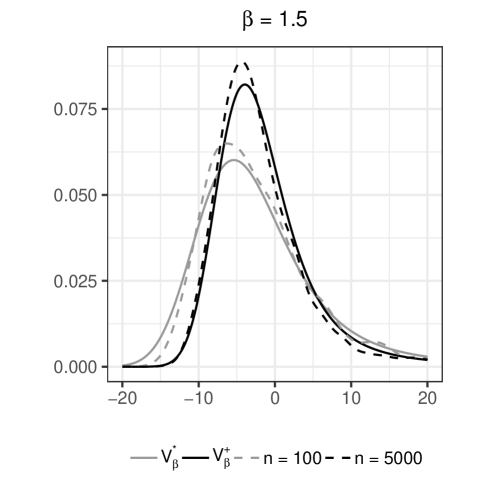
b − 1 𝒵 β ∗ ( b τ ) → fdd { τ V β ∗ as b → 0 , τ V β + as b → ∞ , subscript → fdd superscript 𝑏 1 superscript subscript 𝒵 𝛽 ∗ 𝑏 𝜏 cases 𝜏 subscript superscript 𝑉 ∗ 𝛽 → as 𝑏 0 𝜏 subscript superscript 𝑉 𝛽 → as 𝑏 \displaystyle b^{-1}{\cal Z}_{\beta}^{\ast}(b\tau)\to_{\rm fdd}\begin{cases}\tau V^{\ast}_{\beta}&\text{as }b\to 0,\\
\tau V^{+}_{\beta}&\text{as }b\to\infty,\end{cases} (2.26)
where V β + subscript superscript 𝑉 𝛽 V^{+}_{\beta} , V β ∗ subscript superscript 𝑉 ∗ 𝛽 V^{\ast}_{\beta} are a completely asymmetric β 𝛽 \beta -stable r.v.s with ch.f.s Ee i θ V β + = exp { ψ ( 1 ) ∫ 0 ∞ ( e i θ / ( 2 x ) − 1 − i ( θ / ( 2 x ) ) 𝟏 ( 1 < β < 2 ) ) x β − 1 d x } superscript Ee i 𝜃 subscript superscript 𝑉 𝛽 𝜓 1 superscript subscript 0 superscript e i 𝜃 2 𝑥 1 i 𝜃 2 𝑥 1 1 𝛽 2 superscript 𝑥 𝛽 1 differential-d 𝑥 \mathrm{E}\mathrm{e}^{\mathrm{i}\theta V^{+}_{\beta}}=\exp\{\psi(1)\int_{0}^{\infty}(\mathrm{e}^{\mathrm{i}\theta/(2x)}-1-\mathrm{i}(\theta/(2x)){\bf 1}(1<\beta<2))x^{\beta-1}\mathrm{d}x\} ,
Ee i θ V β ∗ = exp { ψ ( 1 ) ∫ 0 ∞ E ( e i θ Z 2 / ( 2 x ) − 1 − i ( θ Z 2 / ( 2 x ) ) 𝟏 ( 1 < β < 2 ) ) x β − 1 d x } superscript Ee i 𝜃 subscript superscript 𝑉 ∗ 𝛽 𝜓 1 superscript subscript 0 E superscript e i 𝜃 superscript 𝑍 2 2 𝑥 1 i 𝜃 superscript 𝑍 2 2 𝑥 1 1 𝛽 2 superscript 𝑥 𝛽 1 differential-d 𝑥 \mathrm{E}\mathrm{e}^{\mathrm{i}\theta V^{\ast}_{\beta}}=\exp\{\psi(1)\int_{0}^{\infty}\mathrm{E}(\mathrm{e}^{\mathrm{i}\theta Z^{2}/(2x)}-1-\mathrm{i}(\theta Z^{2}/(2x)){\bf 1}(1<\beta<2))x^{\beta-1}\mathrm{d}x\} , θ ∈ ℝ 𝜃 ℝ \theta\in\mathbb{R} and Z ∼ N ( 0 , 1 ) similar-to 𝑍 𝑁 0 1 Z\sim N(0,1) .
2.4. Conditional long-run variance of products of RCAR(1) processes.
We use some facts in Proposition 2.4 Y i j ( t ) := X i ( t ) X j ( t ) assign subscript 𝑌 𝑖 𝑗 𝑡 subscript 𝑋 𝑖 𝑡 subscript 𝑋 𝑗 𝑡 Y_{ij}(t):=X_{i}(t)X_{j}(t) Y i j ( t ) = Y i j + ( t ) + Y i j − ( t ) subscript 𝑌 𝑖 𝑗 𝑡 subscript superscript 𝑌 𝑖 𝑗 𝑡 superscript subscript 𝑌 𝑖 𝑗 𝑡 Y_{ij}(t)=Y^{+}_{ij}(t)+Y_{ij}^{-}(t) Y i j + ( t ) = ∑ s 1 ∧ s 2 ≥ 1 a i t − s 1 a j t − s 2 𝟏 ( t ≥ s 1 ∨ s 2 ) ε i ( s 1 ) ε j ( s 2 ) , Y i j − ( t ) = ∑ s 1 ∧ s 2 ≤ 0 a i t − s 1 a j t − s 2 𝟏 ( t ≥ s 1 ∨ s 2 ) ε i ( s 1 ) ε j ( s 2 ) formulae-sequence superscript subscript 𝑌 𝑖 𝑗 𝑡 subscript subscript 𝑠 1 subscript 𝑠 2 1 superscript subscript 𝑎 𝑖 𝑡 subscript 𝑠 1 superscript subscript 𝑎 𝑗 𝑡 subscript 𝑠 2 1 𝑡 subscript 𝑠 1 subscript 𝑠 2 subscript 𝜀 𝑖 subscript 𝑠 1 subscript 𝜀 𝑗 subscript 𝑠 2 superscript subscript 𝑌 𝑖 𝑗 𝑡 subscript subscript 𝑠 1 subscript 𝑠 2 0 superscript subscript 𝑎 𝑖 𝑡 subscript 𝑠 1 superscript subscript 𝑎 𝑗 𝑡 subscript 𝑠 2 1 𝑡 subscript 𝑠 1 subscript 𝑠 2 subscript 𝜀 𝑖 subscript 𝑠 1 subscript 𝜀 𝑗 subscript 𝑠 2 Y_{ij}^{+}(t)=\sum_{s_{1}\wedge s_{2}\geq 1}a_{i}^{t-s_{1}}a_{j}^{t-s_{2}}{\bf 1}(t\geq s_{1}\vee s_{2})\varepsilon_{i}(s_{1})\varepsilon_{j}(s_{2}),Y_{ij}^{-}(t)=\sum_{s_{1}\wedge s_{2}\leq 0}a_{i}^{t-s_{1}}a_{j}^{t-s_{2}}{\bf 1}(t\geq s_{1}\vee s_{2})\varepsilon_{i}(s_{1})\varepsilon_{j}(s_{2}) i = j 𝑖 𝑗 i=j E ε i 4 ( 0 ) < ∞ E superscript subscript 𝜀 𝑖 4 0 \mathrm{E}\varepsilon_{i}^{4}(0)<\infty
Proposition 2.4 .
We have
var [ ∑ t = 1 n Y i j ( t ) | a i , a j ] var delimited-[] conditional superscript subscript 𝑡 1 𝑛 subscript 𝑌 𝑖 𝑗 𝑡 subscript 𝑎 𝑖 subscript 𝑎 𝑗
\displaystyle{\rm var}\big{[}\sum_{t=1}^{n}Y_{ij}(t)|a_{i},a_{j}\big{]} ∼ similar-to \displaystyle\sim var [ ∑ t = 1 n Y i j + ( t ) | a i , a j ] ∼ A i j n , n → ∞ , formulae-sequence similar-to var delimited-[] conditional superscript subscript 𝑡 1 𝑛 subscript superscript 𝑌 𝑖 𝑗 𝑡 subscript 𝑎 𝑖 subscript 𝑎 𝑗
subscript 𝐴 𝑖 𝑗 𝑛 → 𝑛 \displaystyle{\rm var}\big{[}\sum_{t=1}^{n}Y^{+}_{ij}(t)|a_{i},a_{j}\big{]}\ \sim\ A_{ij}n,\qquad n\to\infty, (2.27)
where
A i j := { 1 + a i a j ( 1 − a i 2 ) ( 1 − a j 2 ) ( 1 − a i a j ) , i ≠ j , 1 + a i 2 1 − a i 2 ( 2 ( 1 − a i 2 ) 2 + cum 4 1 − a i 4 ) , i = j assign subscript 𝐴 𝑖 𝑗 cases 1 subscript 𝑎 𝑖 subscript 𝑎 𝑗 1 superscript subscript 𝑎 𝑖 2 1 superscript subscript 𝑎 𝑗 2 1 subscript 𝑎 𝑖 subscript 𝑎 𝑗 𝑖 𝑗 1 subscript superscript 𝑎 2 𝑖 1 superscript subscript 𝑎 𝑖 2 2 superscript 1 superscript subscript 𝑎 𝑖 2 2 subscript cum 4 1 superscript subscript 𝑎 𝑖 4 𝑖 𝑗 A_{ij}:=\begin{cases}\frac{1+a_{i}a_{j}}{(1-a_{i}^{2})(1-a_{j}^{2})(1-a_{i}a_{j})},&i\neq j,\\
\frac{1+a^{2}_{i}}{1-a_{i}^{2}}(\frac{2}{(1-a_{i}^{2})^{2}}+\frac{{\rm cum}_{4}}{1-a_{i}^{4}}),&i=j\end{cases} (2.28)
with cum 4 subscript cum 4 {\rm cum}_{4} ε i ( 0 ) subscript 𝜀 𝑖 0 \varepsilon_{i}(0) n ≥ 1 , i , j ∈ ℤ , a i , a j ∈ [ 0 , 1 ) formulae-sequence 𝑛 1 𝑖
formulae-sequence 𝑗 ℤ subscript 𝑎 𝑖
subscript 𝑎 𝑗 0 1 n\geq 1,\,i,j\in\mathbb{Z},\ a_{i},a_{j}\in[0,1)
var [ ∑ t = 1 n Y i j ( t ) | a i , a j ] ≤ C i j n 2 ( 1 − a i ) ( 1 − a j ) min { 1 , 1 n ( 2 − a i − a j ) } , var delimited-[] conditional superscript subscript 𝑡 1 𝑛 subscript 𝑌 𝑖 𝑗 𝑡 subscript 𝑎 𝑖 subscript 𝑎 𝑗
subscript 𝐶 𝑖 𝑗 superscript 𝑛 2 1 subscript 𝑎 𝑖 1 subscript 𝑎 𝑗 1 1 𝑛 2 subscript 𝑎 𝑖 subscript 𝑎 𝑗 \displaystyle{\rm var}\big{[}\sum_{t=1}^{n}Y_{ij}(t)|a_{i},a_{j}\big{]}\ \leq\ \frac{C_{ij}n^{2}}{(1-a_{i})(1-a_{j})}\min\big{\{}1,\frac{1}{n(2-a_{i}-a_{j})}\big{\}}, (2.29)
where C i j := 4 ( i ≠ j ) assign subscript 𝐶 𝑖 𝑗 4 𝑖 𝑗 C_{ij}:=4\ (i\neq j) := 2 ( 2 + | cum 4 | ) ( i = j ) assign absent 2 2 subscript cum 4 𝑖 𝑗 :=2(2+|{\rm cum}_{4}|)\ (i=j)
Proof. Let i ≠ j 𝑖 𝑗 i\neq j E [ Y i j ( t ) Y i j ( s ) | a i , a j ] = E [ X i ( t ) X i ( s ) | a i ] E [ X j ( t ) X j ( s ) | a j ] = ( a i a j ) | t − s | / ( 1 − a i 2 ) ( 1 − a j 2 ) E delimited-[] conditional subscript 𝑌 𝑖 𝑗 𝑡 subscript 𝑌 𝑖 𝑗 𝑠 subscript 𝑎 𝑖 subscript 𝑎 𝑗
E delimited-[] conditional subscript 𝑋 𝑖 𝑡 subscript 𝑋 𝑖 𝑠 subscript 𝑎 𝑖 E delimited-[] conditional subscript 𝑋 𝑗 𝑡 subscript 𝑋 𝑗 𝑠 subscript 𝑎 𝑗 superscript subscript 𝑎 𝑖 subscript 𝑎 𝑗 𝑡 𝑠 1 superscript subscript 𝑎 𝑖 2 1 superscript subscript 𝑎 𝑗 2 \mathrm{E}[Y_{ij}(t)Y_{ij}(s)|a_{i},a_{j}]=\mathrm{E}[X_{i}(t)X_{i}(s)|a_{i}]\mathrm{E}[X_{j}(t)X_{j}(s)|a_{j}]=(a_{i}a_{j})^{|t-s|}/(1-a_{i}^{2})(1-a_{j}^{2})
J n ( a i , a j ) := E [ ( ∑ t = 1 n Y i j ( t ) ) 2 | a i , a j ] assign subscript 𝐽 𝑛 subscript 𝑎 𝑖 subscript 𝑎 𝑗 E delimited-[] conditional superscript superscript subscript 𝑡 1 𝑛 subscript 𝑌 𝑖 𝑗 𝑡 2 subscript 𝑎 𝑖 subscript 𝑎 𝑗
\displaystyle J_{n}(a_{i},a_{j}):=\mathrm{E}\big{[}\big{(}\sum_{t=1}^{n}Y_{ij}(t)\big{)}^{2}|a_{i},a_{j}\big{]} = \displaystyle= n ( 1 − a i 2 ) ( 1 − a j 2 ) ∑ t = − n n ( a i a j ) | t | ( 1 − | t | n ) . 𝑛 1 superscript subscript 𝑎 𝑖 2 1 superscript subscript 𝑎 𝑗 2 superscript subscript 𝑡 𝑛 𝑛 superscript subscript 𝑎 𝑖 subscript 𝑎 𝑗 𝑡 1 𝑡 𝑛 \displaystyle\frac{n}{(1-a_{i}^{2})(1-a_{j}^{2})}\sum_{t=-n}^{n}(a_{i}a_{j})^{|t|}\big{(}1-\frac{|t|}{n}\big{)}. (2.30)
Relation (2.30 2.27 J n ( a i , a j ) ≤ 2 n 2 / ( ( 1 − a i ) ( 1 − a j ) ) subscript 𝐽 𝑛 subscript 𝑎 𝑖 subscript 𝑎 𝑗 2 superscript 𝑛 2 1 subscript 𝑎 𝑖 1 subscript 𝑎 𝑗 J_{n}(a_{i},a_{j})\leq 2n^{2}/((1-a_{i})(1-a_{j})) 1 − a i a j ≥ ( 1 / 2 ) ( ( 1 − a i ) + ( 1 − a j ) ) 1 subscript 𝑎 𝑖 subscript 𝑎 𝑗 1 2 1 subscript 𝑎 𝑖 1 subscript 𝑎 𝑗 1-a_{i}a_{j}\geq(1/2)((1-a_{i})+(1-a_{j})) 2.30
J n ( a i , a j ) ≤ n ( 1 − a i 2 ) ( 1 − a j 2 ) ( 1 + 2 ∑ t = 1 ∞ ( a i a j ) t ) ≤ 2 n ( 1 − a i ) ( 1 − a j ) ( 1 − a i a j ) ≤ 4 n ( 1 − a i ) ( 1 − a j ) ( 2 − a i − a j ) , subscript 𝐽 𝑛 subscript 𝑎 𝑖 subscript 𝑎 𝑗 𝑛 1 superscript subscript 𝑎 𝑖 2 1 superscript subscript 𝑎 𝑗 2 1 2 superscript subscript 𝑡 1 superscript subscript 𝑎 𝑖 subscript 𝑎 𝑗 𝑡 2 𝑛 1 subscript 𝑎 𝑖 1 subscript 𝑎 𝑗 1 subscript 𝑎 𝑖 subscript 𝑎 𝑗 4 𝑛 1 subscript 𝑎 𝑖 1 subscript 𝑎 𝑗 2 subscript 𝑎 𝑖 subscript 𝑎 𝑗 J_{n}(a_{i},a_{j})\leq\frac{n}{(1-a_{i}^{2})(1-a_{j}^{2})}\big{(}1+2\sum_{t=1}^{\infty}(a_{i}a_{j})^{t}\big{)}\leq\frac{2n}{(1-a_{i})(1-a_{j})(1-a_{i}a_{j})}\leq\frac{4n}{(1-a_{i})(1-a_{j})(2-a_{i}-a_{j})},
proving (2.29 2.27 2.29 i = j 𝑖 𝑗 i=j cov [ Y i i ( t ) , Y i i ( s ) | a i ] = 2 ( a i | t − s | / ( 1 − a i 2 ) ) 2 + cum 4 a i 2 | t − s | / ( 1 − a i 4 ) . cov subscript 𝑌 𝑖 𝑖 𝑡 conditional subscript 𝑌 𝑖 𝑖 𝑠 subscript 𝑎 𝑖 2 superscript superscript subscript 𝑎 𝑖 𝑡 𝑠 1 superscript subscript 𝑎 𝑖 2 2 subscript cum 4 subscript superscript 𝑎 2 𝑡 𝑠 𝑖 1 subscript superscript 𝑎 4 𝑖 {\rm cov}[Y_{ii}(t),Y_{ii}(s)|a_{i}]=2(a_{i}^{|t-s|}/(1-a_{i}^{2}))^{2}+{\rm cum}_{4}a^{2|t-s|}_{i}/(1-a^{4}_{i}). □ □ \Box
3 Asymptotic distribution of cross-sectional sample covariances
Theorems 3.1 3.2
S N , n t , s ( τ ) := ∑ i = 1 N ∑ u = 1 ⌊ n τ ⌋ X i ( u ) X i + s ( u + t ) , τ ≥ 0 , formulae-sequence assign subscript superscript 𝑆 𝑡 𝑠
𝑁 𝑛
𝜏 superscript subscript 𝑖 1 𝑁 superscript subscript 𝑢 1 𝑛 𝜏 subscript 𝑋 𝑖 𝑢 subscript 𝑋 𝑖 𝑠 𝑢 𝑡 𝜏 0 S^{t,s}_{N,n}(\tau):=\sum_{i=1}^{N}\sum_{u=1}^{\lfloor n\tau\rfloor}X_{i}(u)X_{i+s}(u+t),\quad\tau\geq 0, (3.1)
where t 𝑡 t s ∈ ℤ , s ≠ 0 formulae-sequence 𝑠 ℤ 𝑠 0 s\in\mathbb{Z},s\neq 0 N 𝑁 N n 𝑛 n γ ^ N , n ( t , s ) subscript ^ 𝛾 𝑁 𝑛
𝑡 𝑠 \widehat{\gamma}_{N,n}(t,s) 3.1 t , s 𝑡 𝑠
t,s { X i ( t ) , t ∈ ℤ } , i ∈ ℤ subscript 𝑋 𝑖 𝑡 𝑡
ℤ 𝑖
ℤ \{X_{i}(t),t\in\mathbb{Z}\},i\in\mathbb{Z}
Theorem 3.1 .
Let the mixing distribution satisfy condition (1.2 0 < β < 3 / 2 0 𝛽 3 2 0<\beta<3/2 N , n → ∞ → 𝑁 𝑛
N,n\to\infty
λ N , n := N 1 / ( 2 β ) n → λ ∞ ∈ [ 0 , ∞ ] . assign subscript 𝜆 𝑁 𝑛
superscript 𝑁 1 2 𝛽 𝑛 → subscript 𝜆 0 \lambda_{N,n}:=\frac{N^{1/(2\beta)}}{n}\ \to\lambda_{\infty}\ \in\ [0,\infty]. (3.2)
Then the following statements (i)–(iii) hold for S N , n t , s ( τ ) , ( t , s ) ∈ ℤ 2 , s ≠ 0 formulae-sequence subscript superscript 𝑆 𝑡 𝑠
𝑁 𝑛
𝜏 𝑡 𝑠
superscript ℤ 2 𝑠 0 S^{t,s}_{N,n}(\tau),(t,s)\in\mathbb{Z}^{2},s\neq 0 3.1 λ ∞ subscript 𝜆 \lambda_{\infty} 3.2
(i) Let λ ∞ = ∞ subscript 𝜆 \lambda_{\infty}=\infty . Then
n − 2 λ N , n − β S N , n t , s ( τ ) → fdd σ ∞ B 2 − β ( τ ) , 1 < β < 3 / 2 , superscript 𝑛 2 superscript subscript 𝜆 𝑁 𝑛
𝛽 subscript superscript 𝑆 𝑡 𝑠
𝑁 𝑛
𝜏 subscript → fdd subscript 𝜎 subscript 𝐵 2 𝛽 𝜏 1
𝛽 3 2 \displaystyle\hskip 28.45274ptn^{-2}\lambda_{N,n}^{-\beta}S^{t,s}_{N,n}(\tau)\quad\to_{\rm fdd}\quad\sigma_{\infty}B_{2-\beta}(\tau),\qquad 1<\beta<3/2, (3.3)
n − 2 λ N , n − 1 ( log λ N , n ) − 1 / ( 2 β ) S N , n t , s ( τ ) → fdd τ V 2 β , 0 < β < 1 , formulae-sequence subscript → fdd superscript 𝑛 2 subscript superscript 𝜆 1 𝑁 𝑛
superscript subscript 𝜆 𝑁 𝑛
1 2 𝛽 subscript superscript 𝑆 𝑡 𝑠
𝑁 𝑛
𝜏 𝜏 subscript 𝑉 2 𝛽 0 𝛽 1 \displaystyle n^{-2}\lambda^{-1}_{N,n}(\log\lambda_{N,n})^{-1/(2\beta)}S^{t,s}_{N,n}(\tau)\ \to_{\rm fdd}\ \tau V_{2\beta},\qquad\ 0<\beta<1, (3.4)
where the limit processes are the same as in ( 2.18 ), ( 2.19 ).
(ii) Let λ ∞ = 0 subscript 𝜆 0 \lambda_{\infty}=0 and
E | ε ( 0 ) | 2 p < ∞ E superscript 𝜀 0 2 𝑝 \mathrm{E}|\varepsilon(0)|^{2p}<\infty for some p > 1 𝑝 1 p>1 .
Then
n − 2 λ N , n − 3 / 2 S N , n t , s ( τ ) → fdd 𝒜 1 / 2 B ( τ ) , subscript → fdd superscript 𝑛 2 superscript subscript 𝜆 𝑁 𝑛
3 2 subscript superscript 𝑆 𝑡 𝑠
𝑁 𝑛
𝜏 superscript 𝒜 1 2 𝐵 𝜏 n^{-2}\lambda_{N,n}^{-3/2}S^{t,s}_{N,n}(\tau)\ \to_{\rm fdd}\ {\cal A}^{1/2}B(\tau), (3.5)
where the limit process is the same as in ( 2.20 ).
(iii) Let 0 < λ ∞ < ∞ 0 subscript 𝜆 0<\lambda_{\infty}<\infty . Then
n − 2 λ N , n − 3 / 2 S N , n t , s ( τ ) → fdd λ ∞ 1 / 2 𝒵 β ( τ / λ ∞ ) , subscript → fdd superscript 𝑛 2 superscript subscript 𝜆 𝑁 𝑛
3 2 subscript superscript 𝑆 𝑡 𝑠
𝑁 𝑛
𝜏 superscript subscript 𝜆 1 2 subscript 𝒵 𝛽 𝜏 subscript 𝜆 \displaystyle n^{-2}\lambda_{N,n}^{-3/2}S^{t,s}_{N,n}(\tau)\ \to_{\rm fdd}\ \lambda_{\infty}^{1/2}{\cal Z}_{\beta}(\tau/\lambda_{\infty}), (3.6)
where 𝒵 β subscript 𝒵 𝛽 {\cal Z}_{\beta} is the intermediate process in ( 2.13 ).
Theorem 3.2 .
Let the mixing distribution satisfy condition (1.2 β > 3 / 2 𝛽 3 2 \beta>3/2 E | ε ( 0 ) | 2 p < ∞ E superscript 𝜀 0 2 𝑝 \mathrm{E}|\varepsilon(0)|^{2p}<\infty p > 1 𝑝 1 p>1 ( t , s ) ∈ ℤ 2 , s ≠ 0 formulae-sequence 𝑡 𝑠 superscript ℤ 2 𝑠 0 (t,s)\in\mathbb{Z}^{2},s\neq 0 N , n → ∞ → 𝑁 𝑛
N,n\to\infty
n − 1 / 2 N − 1 / 2 S N , n t , s ( τ ) → fdd σ B ( τ ) , σ 2 := E A 12 , formulae-sequence subscript → fdd superscript 𝑛 1 2 superscript 𝑁 1 2 subscript superscript 𝑆 𝑡 𝑠
𝑁 𝑛
𝜏 𝜎 𝐵 𝜏 assign superscript 𝜎 2 E subscript 𝐴 12 n^{-1/2}N^{-1/2}S^{t,s}_{N,n}(\tau)\ \to_{\rm fdd}\ \sigma B(\tau),\qquad\sigma^{2}:=\mathrm{E}A_{12}, (3.7)
where A 12 subscript 𝐴 12 A_{12} 2.28
Note that the asymptotic distribution of sample covariances γ ^ N , n ( t , s ) subscript ^ 𝛾 𝑁 𝑛
𝑡 𝑠 \widehat{\gamma}_{N,n}(t,s) 1.5
γ ~ N , n ( t , s ) := ( N n ) − 1 S N , n t , s ( 1 ) − ( X ¯ N , n ) 2 . assign subscript ~ 𝛾 𝑁 𝑛
𝑡 𝑠 superscript 𝑁 𝑛 1 subscript superscript 𝑆 𝑡 𝑠
𝑁 𝑛
1 superscript subscript ¯ 𝑋 𝑁 𝑛
2 \widetilde{\gamma}_{N,n}(t,s):=(Nn)^{-1}S^{t,s}_{N,n}(1)-(\bar{X}_{N,n})^{2}. (3.8)
For s ≠ 0 𝑠 0 s\neq 0 3.8 3.1 3.2 β 𝛽 \beta X ¯ N , n subscript ¯ 𝑋 𝑁 𝑛
\bar{X}_{N,n} [20 ]
and is given in the following proposition, with some simplifications.
Proposition 3.1 .
Let the mixing distribution satisfy condition (1.2 β > 0 𝛽 0 \beta>0
(i) Let 1 < β < 2 1 𝛽 2 1<\beta<2 and N / n β → ∞ → 𝑁 superscript 𝑛 𝛽 N/n^{\beta}\to\infty . Then
N 1 / 2 n ( β − 1 ) / 2 X ¯ N , n → d σ ¯ β Z , subscript → d superscript 𝑁 1 2 superscript 𝑛 𝛽 1 2 subscript ¯ 𝑋 𝑁 𝑛
subscript ¯ 𝜎 𝛽 𝑍 \displaystyle N^{1/2}n^{(\beta-1)/2}\bar{X}_{N,n}\to_{\rm d}\bar{\sigma}_{\beta}Z, (3.9)
where Z ∼ N ( 0 , 1 ) similar-to 𝑍 𝑁 0 1 Z\sim N(0,1) and σ ¯ β 2 := ψ ( 1 ) Γ ( β − 1 ) / ( ( 3 − β ) ( 2 − β ) ) assign subscript superscript ¯ 𝜎 2 𝛽 𝜓 1 Γ 𝛽 1 3 𝛽 2 𝛽 \bar{\sigma}^{2}_{\beta}:=\psi(1)\Gamma(\beta-1)/((3-\beta)(2-\beta)) .
(ii) Let 0 < β < 1 0 𝛽 1 0<\beta<1 and N / n β → ∞ → 𝑁 superscript 𝑛 𝛽 N/n^{\beta}\to\infty . Then
N 1 − 1 / 2 β X ¯ N , n → d V ¯ 2 β , subscript → d superscript 𝑁 1 1 2 𝛽 subscript ¯ 𝑋 𝑁 𝑛
subscript ¯ 𝑉 2 𝛽 \displaystyle N^{1-1/2\beta}\bar{X}_{N,n}\to_{\rm d}\bar{V}_{2\beta}, (3.10)
where V ¯ 2 β subscript ¯ 𝑉 2 𝛽 \bar{V}_{2\beta} is a symmetric ( 2 β ) 2 𝛽 (2\beta) -stable r.v. with ch.f. Ee i θ V ¯ 2 β = e − K ¯ β | θ | 2 β , K ¯ β := ψ ( 1 ) 4 − β Γ ( 1 − β ) / β formulae-sequence superscript Ee i 𝜃 subscript ¯ 𝑉 2 𝛽 superscript e subscript ¯ 𝐾 𝛽 superscript 𝜃 2 𝛽 assign subscript ¯ 𝐾 𝛽 𝜓 1 superscript 4 𝛽 Γ 1 𝛽 𝛽 \mathrm{E}\mathrm{e}^{\mathrm{i}\theta\bar{V}_{2\beta}}=\mathrm{e}^{-\bar{K}_{\beta}|\theta|^{2\beta}},\bar{K}_{\beta}:=\psi(1)4^{-\beta}\Gamma(1-\beta)/\beta .
(iii) Let 0 < β < 2 0 𝛽 2 0<\beta<2 and N / n β → 0 → 𝑁 superscript 𝑛 𝛽 0 N/n^{\beta}\to 0 . Then
N 1 − 1 / β n 1 / 2 X ¯ N , n → d W ¯ β , subscript → d superscript 𝑁 1 1 𝛽 superscript 𝑛 1 2 subscript ¯ 𝑋 𝑁 𝑛
subscript ¯ 𝑊 𝛽 \displaystyle N^{1-1/\beta}n^{1/2}\bar{X}_{N,n}\to_{\rm d}\bar{W}_{\beta}, (3.11)
where W ¯ β subscript ¯ 𝑊 𝛽 \bar{W}_{\beta} is a symmetric β 𝛽 \beta -stable r.v. with ch.f. Ee i θ W ¯ β = e − k ¯ β | θ | β , k ¯ β := ψ ( 1 ) 2 − β / 2 Γ ( 1 − β / 2 ) / β formulae-sequence superscript Ee i 𝜃 subscript ¯ 𝑊 𝛽 superscript e subscript ¯ 𝑘 𝛽 superscript 𝜃 𝛽 assign subscript ¯ 𝑘 𝛽 𝜓 1 superscript 2 𝛽 2 Γ 1 𝛽 2 𝛽 \mathrm{E}\mathrm{e}^{\mathrm{i}\theta\bar{W}_{\beta}}=\mathrm{e}^{-\bar{k}_{\beta}|\theta|^{\beta}},\bar{k}_{\beta}:=\psi(1)2^{-\beta/2}\Gamma(1-\beta/2)/\beta .
(iv) Let β > 2 𝛽 2 \beta>2 . Then as N , n → ∞ → 𝑁 𝑛
N,n\to\infty in arbitrary way,
N 1 / 2 n 1 / 2 X ¯ N , n → d σ ¯ Z , subscript → d superscript 𝑁 1 2 superscript 𝑛 1 2 subscript ¯ 𝑋 𝑁 𝑛
¯ 𝜎 𝑍 \displaystyle N^{1/2}n^{1/2}\bar{X}_{N,n}\to_{\rm d}\bar{\sigma}Z, (3.12)
where Z ∼ N ( 0 , 1 ) similar-to 𝑍 𝑁 0 1 Z\sim N(0,1) and σ ¯ 2 := E ( 1 − a ) − 2 assign superscript ¯ 𝜎 2 E superscript 1 𝑎 2 \bar{\sigma}^{2}:=\mathrm{E}(1-a)^{-2} .
From Theorems 3.1 3.1 3.8 two ‘bifurcation points’ of the limit behavior, viz.,
as N ∼ n 2 β similar-to 𝑁 superscript 𝑛 2 𝛽 N\sim n^{2\beta} N ∼ n β similar-to 𝑁 superscript 𝑛 𝛽 N\sim n^{\beta} β 𝛽 \beta γ ^ N , n ( t , s ) subscript ^ 𝛾 𝑁 𝑛
𝑡 𝑠 \widehat{\gamma}_{N,n}(t,s) β 𝛽 \beta both terms on the r.h.s. may contribute to the limit.
Essentially, the corollary follows by comparing the normalizations
in Theorems 3.1 3.1
Corollary 3.1 .
Assume that the mixing distribution satisfies condition (1.2 β > 0 𝛽 0 \beta>0 E | ε ( 0 ) | 2 p < ∞ E superscript 𝜀 0 2 𝑝 \mathrm{E}|\varepsilon(0)|^{2p}<\infty p > 1 𝑝 1 p>1 ( t , s ) ∈ ℤ 2 , s ≠ 0 formulae-sequence 𝑡 𝑠 superscript ℤ 2 𝑠 0 (t,s)\in\mathbb{Z}^{2},s\neq 0
(i) Let N / n 2 β → ∞ → 𝑁 superscript 𝑛 2 𝛽 N/n^{2\beta}\to\infty and 1 < β < 3 / 2 1 𝛽 3 2 1<\beta<3/2 . Then
N 1 / 2 n β − 1 γ ^ N , n ( t , s ) → d σ ∞ Z , subscript → d superscript 𝑁 1 2 superscript 𝑛 𝛽 1 subscript ^ 𝛾 𝑁 𝑛
𝑡 𝑠 subscript 𝜎 𝑍 \displaystyle N^{1/2}n^{\beta-1}\widehat{\gamma}_{N,n}(t,s)\ \to_{\rm d}\ \sigma_{\infty}Z,
where Z ∼ N ( 0 , 1 ) similar-to 𝑍 𝑁 0 1 Z\sim N(0,1) and σ ∞ subscript 𝜎 \sigma_{\infty} is the same as in Theorem 3.1 (i).
(ii) Let N / n 2 β → ∞ → 𝑁 superscript 𝑛 2 𝛽 N/n^{2\beta}\to\infty and 1 / 2 < β < 1 1 2 𝛽 1 1/2<\beta<1 . Then
N 1 − 1 / ( 2 β ) log 1 / ( 2 β ) ( N 1 / ( 2 β ) / n ) γ ^ N , n ( t , s ) → d V 2 β , subscript → d superscript 𝑁 1 1 2 𝛽 superscript 1 2 𝛽 superscript 𝑁 1 2 𝛽 𝑛 subscript ^ 𝛾 𝑁 𝑛
𝑡 𝑠 subscript 𝑉 2 𝛽 \displaystyle\frac{N^{1-1/(2\beta)}}{\log^{1/(2\beta)}(N^{1/(2\beta)}/n)}\,\widehat{\gamma}_{N,n}(t,s)\to_{\rm d}V_{2\beta},
where V 2 β subscript 𝑉 2 𝛽 V_{2\beta} is symmetric ( 2 β ) 2 𝛽 (2\beta) -stable r.v. defined in Theorem 3.1 (i).
(iii) Let N / n 2 β → ∞ → 𝑁 superscript 𝑛 2 𝛽 N/n^{2\beta}\to\infty and 0 < β < 1 / 2 0 𝛽 1 2 0<\beta<1/2 . Then
N 2 − 1 / β γ ^ N , n ( t , s ) → d − ( V ¯ 2 β ) 2 , subscript → d superscript 𝑁 2 1 𝛽 subscript ^ 𝛾 𝑁 𝑛
𝑡 𝑠 superscript subscript ¯ 𝑉 2 𝛽 2 \displaystyle N^{2-1/\beta}\widehat{\gamma}_{N,n}(t,s)\to_{\rm d}-(\bar{V}_{2\beta})^{2}, (3.13)
where V ¯ 2 β subscript ¯ 𝑉 2 𝛽 \bar{V}_{2\beta} is symmetric ( 2 β ) 2 𝛽 (2\beta) -stable r.v. defined in Proposition 3.1 (ii).
(iv) Let N / n 2 β → 0 , N / n β → ∞ formulae-sequence → 𝑁 superscript 𝑛 2 𝛽 0 → 𝑁 superscript 𝑛 𝛽 N/n^{2\beta}\to 0,N/n^{\beta}\to\infty and 3 / 4 < β < 3 / 2 3 4 𝛽 3 2 3/4<\beta<3/2 . Then
N 1 − 3 / ( 4 β ) n 1 / 2 γ ^ N , n ( t , s ) → d W 4 β / 3 , subscript → d superscript 𝑁 1 3 4 𝛽 superscript 𝑛 1 2 subscript ^ 𝛾 𝑁 𝑛
𝑡 𝑠 subscript 𝑊 4 𝛽 3 \displaystyle N^{1-3/(4\beta)}n^{1/2}\widehat{\gamma}_{N,n}(t,s)\ \to_{\rm d}\ W_{4\beta/3}, (3.14)
where W 4 β / 3 subscript 𝑊 4 𝛽 3 W_{4\beta/3} is a symmetric ( 4 β / 3 ) 4 𝛽 3 (4\beta/3) -stable r.v. with
characteristic function Ee i θ W 4 β / 3 = e − ( σ 0 / 2 2 β / 3 ) | θ | 4 β / 3 superscript Ee i 𝜃 subscript 𝑊 4 𝛽 3 superscript e subscript 𝜎 0 superscript 2 2 𝛽 3 superscript 𝜃 4 𝛽 3 \mathrm{E}\mathrm{e}^{\mathrm{i}\theta W_{4\beta/3}}=\mathrm{e}^{-(\sigma_{0}/2^{2\beta/3})|\theta|^{4\beta/3}}
and σ 0 subscript 𝜎 0 \sigma_{0} is the same constant as in Theorem 3.1 (ii).
(v) Let N / n 2 β → 0 , 1 / 2 < β < 3 / 4 formulae-sequence → 𝑁 superscript 𝑛 2 𝛽 0 1 2 𝛽 3 4 N/n^{2\beta}\to 0,1/2<\beta<3/4 and N / n 2 β / ( 4 β − 1 ) → ∞ → 𝑁 superscript 𝑛 2 𝛽 4 𝛽 1 N/n^{2\beta/(4\beta-1)}\to\infty .
Then the convergence in ( 3.14 ) holds.
(vi) Let N / n β → ∞ , 1 / 2 < β < 3 / 4 formulae-sequence → 𝑁 superscript 𝑛 𝛽 1 2 𝛽 3 4 N/n^{\beta}\to\infty,1/2<\beta<3/4 and N / n 2 β / ( 4 β − 1 ) → 0 → 𝑁 superscript 𝑛 2 𝛽 4 𝛽 1 0 N/n^{2\beta/(4\beta-1)}\to 0 .
Then the convergence in ( 3.13 ) holds.
(vii) Let N / n 2 β → 0 , N / n β → ∞ formulae-sequence → 𝑁 superscript 𝑛 2 𝛽 0 → 𝑁 superscript 𝑛 𝛽 N/n^{2\beta}\to 0,N/n^{\beta}\to\infty and 0 < β < 1 / 2 0 𝛽 1 2 0<\beta<1/2 .
Then the convergence in ( 3.13 ) holds.
(viii) Let N / n β → 0 → 𝑁 superscript 𝑛 𝛽 0 N/n^{\beta}\to 0 and 3 / 4 < β < 3 / 2 3 4 𝛽 3 2 3/4<\beta<3/2 .
Then the convergence in ( 3.14 ) holds.
(ix) Let N / n β → 0 , 0 < β < 3 / 4 formulae-sequence → 𝑁 superscript 𝑛 𝛽 0 0 𝛽 3 4 N/n^{\beta}\to 0,0<\beta<3/4 and N / n 2 β / ( 5 − 4 β ) → ∞ → 𝑁 superscript 𝑛 2 𝛽 5 4 𝛽 N/n^{2\beta/(5-4\beta)}\to\infty .
Then
N 2 − 2 / β γ ^ N , n ( t , s ) → d − ( W ¯ β ) 2 , subscript → d superscript 𝑁 2 2 𝛽 subscript ^ 𝛾 𝑁 𝑛
𝑡 𝑠 superscript subscript ¯ 𝑊 𝛽 2 \displaystyle N^{2-2/\beta}\widehat{\gamma}_{N,n}(t,s)\to_{\rm d}-(\bar{W}_{\beta})^{2}, (3.15)
where W ¯ β subscript ¯ 𝑊 𝛽 \bar{W}_{\beta} is a symmetric β 𝛽 \beta -stable r.v. defined in Proposition 3.1 (iii).
(x) Let 0 < β < 3 / 4 0 𝛽 3 4 0<\beta<3/4 and N / n 2 β / ( 5 − 4 β ) → 0 → 𝑁 superscript 𝑛 2 𝛽 5 4 𝛽 0 N/n^{2\beta/(5-4\beta)}\to 0 .
Then the convergence in ( 3.14 ) holds.
(xi) For 3 / 2 < β < 2 3 2 𝛽 2 3/2<\beta<2 , let N / n β → [ 0 , ∞ ] → 𝑁 superscript 𝑛 𝛽 0 N/n^{\beta}\to[0,\infty] and for β > 2 𝛽 2 \beta>2 , let N , n → ∞ → 𝑁 𝑛
N,n\to\infty in arbitrary way. Then
N 1 / 2 n 1 / 2 γ ^ N , n ( t , s ) → d N ( 0 , σ 2 ) , subscript → d superscript 𝑁 1 2 superscript 𝑛 1 2 subscript ^ 𝛾 𝑁 𝑛
𝑡 𝑠 𝑁 0 superscript 𝜎 2 \displaystyle N^{1/2}n^{1/2}\widehat{\gamma}_{N,n}(t,s)\to_{\rm d}N(0,\sigma^{2}), (3.16)
where σ 2 superscript 𝜎 2 \sigma^{2} is given as in Theorem 3.2 .
The proof of Theorem 3.1 3.1 3.3 ( t , s ) = ( 0 , 1 ) 𝑡 𝑠 0 1 (t,s)=(0,1) S N , n ( τ ) := ∑ i = 1 N ∑ t = 1 ⌊ n τ ⌋ X i ( t ) X i + 1 ( t ) assign subscript 𝑆 𝑁 𝑛
𝜏 superscript subscript 𝑖 1 𝑁 superscript subscript 𝑡 1 𝑛 𝜏 subscript 𝑋 𝑖 𝑡 subscript 𝑋 𝑖 1 𝑡 S_{N,n}(\tau):=\sum_{i=1}^{N}\sum_{t=1}^{\lfloor n\tau\rfloor}X_{i}(t)X_{i+1}(t) ( t , s ) , s ≠ 0 𝑡 𝑠 𝑠
0 (t,s),s\neq 0
Let us give an outline of the proof of Theorem 3.1 [20 ] we use the method
of characteristic function combined with ‘vertical’ Bernstein’s blocks, due to the fact that
S N , n subscript 𝑆 𝑁 𝑛
S_{N,n} [20 ] . Write
S N , n ( τ ) = S N , n ; q ( τ ) + S N , n ; q † ( τ ) + S N , n ; q ‡ ( τ ) , subscript 𝑆 𝑁 𝑛
𝜏 subscript 𝑆 𝑁 𝑛 𝑞
𝜏 subscript superscript 𝑆 † 𝑁 𝑛 𝑞
𝜏 subscript superscript 𝑆 ‡ 𝑁 𝑛 𝑞
𝜏 S_{N,n}(\tau)=S_{N,n;q}(\tau)+S^{\dagger}_{N,n;q}(\tau)+S^{\ddagger}_{N,n;q}(\tau), (3.17)
where the main term
S N , n ; q ( τ ) subscript 𝑆 𝑁 𝑛 𝑞
𝜏 \displaystyle S_{N,n;q}(\tau) := assign \displaystyle:= ∑ k = 1 N ~ q Y k , n ; q ( τ ) , Y k , n ; q ( τ ) := ∑ ( k − 1 ) q < i < k q ∑ t = 1 ⌊ n τ ⌋ X i ( t ) X i + 1 ( t ) , 1 ≤ k ≤ N ~ q := ⌊ N q ⌋ , formulae-sequence assign superscript subscript 𝑘 1 subscript ~ 𝑁 𝑞 subscript 𝑌 𝑘 𝑛 𝑞
𝜏 subscript 𝑌 𝑘 𝑛 𝑞
𝜏
subscript 𝑘 1 𝑞 𝑖 𝑘 𝑞 superscript subscript 𝑡 1 𝑛 𝜏 subscript 𝑋 𝑖 𝑡 subscript 𝑋 𝑖 1 𝑡 1 𝑘 subscript ~ 𝑁 𝑞 assign 𝑁 𝑞 \displaystyle\sum_{k=1}^{\tilde{N}_{q}}Y_{k,n;q}(\tau),\quad Y_{k,n;q}(\tau)\ :=\ \sum_{(k-1)q<i<kq}\sum_{t=1}^{\lfloor n\tau\rfloor}X_{i}(t)X_{i+1}(t),\ 1\leq k\leq\tilde{N}_{q}:=\big{\lfloor}\frac{N}{q}\big{\rfloor}, (3.18)
is a sum of N ~ q subscript ~ 𝑁 𝑞 \tilde{N}_{q} q − 1 𝑞 1 q-1
q ≡ q N , n → ∞ as N , n → ∞ . formulae-sequence 𝑞 subscript 𝑞 𝑁 𝑛
→ → as 𝑁 𝑛
q\equiv q_{N,n}\to\infty\qquad\text{as}\quad N,n\to\infty. (3.19)
The convergence rate of q ∈ ℕ 𝑞 ℕ q\in\mathbb{N} 3.19 q = O ( log N ) 𝑞 𝑂 𝑁 q=O(\log N) 3.17
S N , n ; q † ( τ ) := ∑ k = 1 N ~ q ∑ t = 1 ⌊ n τ ⌋ X k q ( t ) X k q + 1 ( t ) , S N , n ; q ‡ ( τ ) := ∑ q N ~ q < i ≤ N ∑ t = 1 ⌊ n τ ⌋ X i ( t ) X i + 1 ( t ) , formulae-sequence assign subscript superscript 𝑆 † 𝑁 𝑛 𝑞
𝜏 superscript subscript 𝑘 1 subscript ~ 𝑁 𝑞 superscript subscript 𝑡 1 𝑛 𝜏 subscript 𝑋 𝑘 𝑞 𝑡 subscript 𝑋 𝑘 𝑞 1 𝑡 assign subscript superscript 𝑆 ‡ 𝑁 𝑛 𝑞
𝜏 subscript 𝑞 subscript ~ 𝑁 𝑞 𝑖 𝑁 superscript subscript 𝑡 1 𝑛 𝜏 subscript 𝑋 𝑖 𝑡 subscript 𝑋 𝑖 1 𝑡 \displaystyle S^{\dagger}_{N,n;q}(\tau)\ :=\ \sum_{k=1}^{\tilde{N}_{q}}\sum_{t=1}^{\lfloor n\tau\rfloor}X_{kq}(t)X_{kq+1}(t),\quad S^{\ddagger}_{N,n;q}(\tau)\ :=\ \sum_{q\tilde{N}_{q}<i\leq N}\sum_{t=1}^{\lfloor n\tau\rfloor}X_{i}(t)X_{i+1}(t), (3.20)
contain respectively N ~ q = o ( N ) subscript ~ 𝑁 𝑞 𝑜 𝑁 \tilde{N}_{q}=o(N) N − q N ~ q < q = o ( N ) 𝑁 𝑞 subscript ~ 𝑁 𝑞 𝑞 𝑜 𝑁 N-q\tilde{N}_{q}<q=o(N) 3.1
A N , n − 1 S N , n ; q ( τ ) → fdd 𝒮 β ( τ ) , subscript → fdd subscript superscript 𝐴 1 𝑁 𝑛
subscript 𝑆 𝑁 𝑛 𝑞
𝜏 subscript 𝒮 𝛽 𝜏 \displaystyle A^{-1}_{N,n}S_{N,n;q}(\tau)\ \to_{\rm fdd}\ {\cal S}_{\beta}(\tau), (3.21)
A N , n − 1 S N , n ; q † ( τ ) = o p ( 1 ) , A N , n − 1 S N , n ; q ‡ ( τ ) = o p ( 1 ) , formulae-sequence subscript superscript 𝐴 1 𝑁 𝑛
subscript superscript 𝑆 † 𝑁 𝑛 𝑞
𝜏 subscript 𝑜 p 1 subscript superscript 𝐴 1 𝑁 𝑛
subscript superscript 𝑆 ‡ 𝑁 𝑛 𝑞
𝜏 subscript 𝑜 p 1 \displaystyle A^{-1}_{N,n}S^{\dagger}_{N,n;q}(\tau)=o_{\rm p}(1),\qquad A^{-1}_{N,n}S^{\ddagger}_{N,n;q}(\tau)=o_{\rm p}(1), (3.22)
where A N , n subscript 𝐴 𝑁 𝑛
A_{N,n} 𝒮 β subscript 𝒮 𝛽 {\cal S}_{\beta}
A N , n := n 2 { λ N , n β , λ ∞ = ∞ , 1 < β < 3 / 2 , λ N , n ( log λ N , n ) 1 / ( 2 β ) , λ ∞ = ∞ , 0 < β < 1 , λ N , n 3 / 2 , λ ∞ ∈ [ 0 , ∞ ) , 0 < β < 3 / 2 . assign subscript 𝐴 𝑁 𝑛
superscript 𝑛 2 cases superscript subscript 𝜆 𝑁 𝑛
𝛽 formulae-sequence subscript 𝜆 1 𝛽 3 2 subscript 𝜆 𝑁 𝑛
superscript subscript 𝜆 𝑁 𝑛
1 2 𝛽 formulae-sequence subscript 𝜆 0 𝛽 1 superscript subscript 𝜆 𝑁 𝑛
3 2 formulae-sequence subscript 𝜆 0 0 𝛽 3 2 \displaystyle A_{N,n}\ :=\ n^{2}\begin{cases}\lambda_{N,n}^{\beta},&\lambda_{\infty}=\infty,\ 1<\beta<3/2,\\
\lambda_{N,n}(\log\lambda_{N,n})^{1/(2\beta)},&\lambda_{\infty}=\infty,\ 0<\beta<1,\\
\lambda_{N,n}^{3/2},&\lambda_{\infty}\in[0,\infty),\ 0<\beta<3/2.\end{cases} (3.23)
Note that the summands Y k , n ; q , 1 ≤ k ≤ N ~ q subscript 𝑌 𝑘 𝑛 𝑞
1
𝑘 subscript ~ 𝑁 𝑞 Y_{k,n;q},1\leq k\leq\tilde{N}_{q} 3.18 , and the limit
𝒮 β ( τ ) subscript 𝒮 𝛽 𝜏 {\cal S}_{\beta}(\tau) 3.1 3.21 τ > 0 𝜏 0 \tau>0 3.21 τ > 0 𝜏 0 \tau>0
Φ N , n ; q ( θ ) → Φ ( θ ) , as N , n → ∞ , λ N , n → λ ∞ , ∀ θ ∈ ℝ , formulae-sequence → subscript Φ 𝑁 𝑛 𝑞
𝜃 Φ 𝜃 as 𝑁
formulae-sequence → 𝑛 formulae-sequence → subscript 𝜆 𝑁 𝑛
subscript 𝜆 for-all 𝜃 ℝ \displaystyle\Phi_{N,n;q}({\theta})\ \rightarrow\ \Phi({\theta}),\quad\text{as}\ N,\,n\to\infty,\,\lambda_{N,n}\to\lambda_{\infty},\quad\forall\theta\in\mathbb{R}, (3.24)
where
Φ N , n ; q ( θ ) := N ~ q E [ e i θ A N , n − 1 Y 1 , n ; q ( τ ) − 1 ] , Φ ( θ ) := log Ee i θ 𝒮 β ( τ ) . formulae-sequence assign subscript Φ 𝑁 𝑛 𝑞
𝜃 subscript ~ 𝑁 𝑞 E delimited-[] superscript e i 𝜃 subscript superscript 𝐴 1 𝑁 𝑛
subscript 𝑌 1 𝑛 𝑞
𝜏 1 assign Φ 𝜃 superscript Ee i 𝜃 subscript 𝒮 𝛽 𝜏 \displaystyle\Phi_{N,n;q}(\theta):=\tilde{N}_{q}\mathrm{E}\big{[}\mathrm{e}^{\mathrm{i}\theta A^{-1}_{N,n}Y_{1,n;q}(\tau)}-1\big{]},\qquad\Phi(\theta):=\log\mathrm{E}\mathrm{e}^{\mathrm{i}\theta{\cal S}_{\beta}(\tau)}. (3.25)
To prove (3.24
A N , n − 1 Y 1 , n ; q ( τ ) = ∑ i = 1 q − 1 y i ( τ ) , where y i ( τ ) := A N , n − 1 ∑ t = 1 ⌊ n τ ⌋ X i ( t ) X i + 1 ( t ) . formulae-sequence subscript superscript 𝐴 1 𝑁 𝑛
subscript 𝑌 1 𝑛 𝑞
𝜏 superscript subscript 𝑖 1 𝑞 1 subscript 𝑦 𝑖 𝜏 where
assign subscript 𝑦 𝑖 𝜏 subscript superscript 𝐴 1 𝑁 𝑛
superscript subscript 𝑡 1 𝑛 𝜏 subscript 𝑋 𝑖 𝑡 subscript 𝑋 𝑖 1 𝑡 \displaystyle A^{-1}_{N,n}Y_{1,n;q}(\tau)=\sum_{i=1}^{q-1}y_{i}(\tau),\quad\text{where}\quad y_{i}(\tau):=A^{-1}_{N,n}\sum_{t=1}^{\lfloor n\tau\rfloor}X_{i}(t)X_{i+1}(t). (3.26)
We use the identity:
∏ 1 ≤ i < q ( 1 + w i ) − 1 = ∑ 1 ≤ i < q w i + ∑ | D | ≥ 2 ∏ i ∈ D w i , subscript product 1 𝑖 𝑞 1 subscript 𝑤 𝑖 1 subscript 1 𝑖 𝑞 subscript 𝑤 𝑖 subscript 𝐷 2 subscript product 𝑖 𝐷 subscript 𝑤 𝑖 \displaystyle\prod_{1\leq i<q}(1+w_{i})-1=\sum_{1\leq i<q}w_{i}+\sum_{|D|\geq 2}\prod_{i\in D}w_{i}, (3.27)
where the sum ∑ | D | ≥ 2 subscript 𝐷 2 \sum_{|D|\geq 2} D ⊂ { 1 , … , q − 1 } 𝐷 1 … 𝑞 1 D\subset\{1,\dots,q-1\} | D | ≥ 2 𝐷 2 |D|\geq 2 3.27 w i = e i θ y i ( τ ) − 1 subscript 𝑤 𝑖 superscript e i 𝜃 subscript 𝑦 𝑖 𝜏 1 w_{i}=\mathrm{e}^{\mathrm{i}\theta y_{i}(\tau)}-1
Φ N , n ; q ( θ ) := N ~ q ( q − 1 ) [ Ee i θ y 1 ( τ ) − 1 ] + N ~ q ∑ | D | ≥ 2 E ∏ i ∈ D [ e i θ y i ( τ ) − 1 ] . assign subscript Φ 𝑁 𝑛 𝑞
𝜃 subscript ~ 𝑁 𝑞 𝑞 1 delimited-[] superscript Ee i 𝜃 subscript 𝑦 1 𝜏 1 subscript ~ 𝑁 𝑞 subscript 𝐷 2 E subscript product 𝑖 𝐷 delimited-[] superscript e i 𝜃 subscript 𝑦 𝑖 𝜏 1 \displaystyle\Phi_{N,n;q}(\theta):=\tilde{N}_{q}(q-1)\big{[}\mathrm{E}\mathrm{e}^{\mathrm{i}\theta y_{1}(\tau)}-1\big{]}+\tilde{N}_{q}\sum_{|D|\geq 2}\mathrm{E}\prod_{i\in D}\big{[}\mathrm{e}^{\mathrm{i}\theta y_{i}(\tau)}-1\big{]}. (3.28)
Thus, since N ~ q ( q − 1 ) / N → 1 → subscript ~ 𝑁 𝑞 𝑞 1 𝑁 1 \tilde{N}_{q}(q-1)/N\to 1 3.24
N [ Ee i θ y 1 ( τ ) − 1 ] 𝑁 delimited-[] superscript Ee i 𝜃 subscript 𝑦 1 𝜏 1 \displaystyle N\big{[}\mathrm{E}\mathrm{e}^{\mathrm{i}\theta y_{1}(\tau)}-1\big{]} → → \displaystyle\to Φ ( θ ) , Φ 𝜃 \displaystyle\Phi(\theta), (3.29)
N ∑ | D | ≥ 2 E ∏ i ∈ D [ e i θ y i ( τ ) − 1 ] 𝑁 subscript 𝐷 2 E subscript product 𝑖 𝐷 delimited-[] superscript e i 𝜃 subscript 𝑦 𝑖 𝜏 1 \displaystyle N\sum_{|D|\geq 2}\mathrm{E}\prod_{i\in D}\big{[}\mathrm{e}^{\mathrm{i}\theta y_{i}(\tau)}-1\big{]} → → \displaystyle\to 0 . 0 \displaystyle 0. (3.30)
Let us explain the main idea of the proof of (3.29 ϕ ( x ) = ( 1 − x ) β − 1 italic-ϕ 𝑥 superscript 1 𝑥 𝛽 1 \phi(x)=(1-x)^{\beta-1} 1.2 3.29
N [ Ee i θ y 1 ( τ ) − 1 ] 𝑁 delimited-[] superscript Ee i 𝜃 subscript 𝑦 1 𝜏 1 \displaystyle N\big{[}\mathrm{E}\mathrm{e}^{\mathrm{i}\theta y_{1}(\tau)}-1\big{]} = \displaystyle= N ∫ ( 0 , 1 ] 2 E [ e i θ y 1 ( τ ) − 1 | a i = 1 − z i , i = 1 , 2 ] ( z 1 z 2 ) β − 1 d z 1 d z 2 𝑁 subscript superscript 0 1 2 E delimited-[] formulae-sequence superscript e i 𝜃 subscript 𝑦 1 𝜏 conditional 1 subscript 𝑎 𝑖 1 subscript 𝑧 𝑖 𝑖 1 2
superscript subscript 𝑧 1 subscript 𝑧 2 𝛽 1 differential-d subscript 𝑧 1 differential-d subscript 𝑧 2 \displaystyle N\int_{(0,1]^{2}}\mathrm{E}\big{[}\mathrm{e}^{\mathrm{i}\theta y_{1}(\tau)}-1\big{|}a_{i}=1-z_{i},i=1,2\big{]}(z_{1}z_{2})^{\beta-1}\mathrm{d}z_{1}\mathrm{d}z_{2} (3.31)
= \displaystyle= N B N , n 2 β ∫ ( 0 , B N , n ] 2 E [ e i θ z N , n ( τ ; x 1 , x 2 ) − 1 ] ( x 1 x 2 ) β − 1 d x 1 d x 2 , 𝑁 subscript superscript 𝐵 2 𝛽 𝑁 𝑛
subscript superscript 0 subscript 𝐵 𝑁 𝑛
2 E delimited-[] superscript e i 𝜃 subscript 𝑧 𝑁 𝑛
𝜏 subscript 𝑥 1 subscript 𝑥 2
1 superscript subscript 𝑥 1 subscript 𝑥 2 𝛽 1 differential-d subscript 𝑥 1 differential-d subscript 𝑥 2 \displaystyle\frac{N}{B^{2\beta}_{N,n}}\int_{(0,B_{N,n}]^{2}}\mathrm{E}\big{[}\mathrm{e}^{\mathrm{i}\theta z_{N,n}(\tau;x_{1},x_{2})}-1\big{]}(x_{1}x_{2})^{\beta-1}\mathrm{d}x_{1}\mathrm{d}x_{2},
where
z N , n ( τ ; x 1 , x 2 ) subscript 𝑧 𝑁 𝑛
𝜏 subscript 𝑥 1 subscript 𝑥 2
\displaystyle z_{N,n}(\tau;x_{1},x_{2}) := assign \displaystyle:= A N , n − 1 ∑ s 1 , s 2 ∈ ℤ ε 1 ( s 1 ) ε 2 ( s 2 ) ∑ t = 1 ⌊ n τ ⌋ ∏ i = 1 2 ( 1 − x i B N , n ) t − s i 𝟏 ( t ≥ s i ) subscript superscript 𝐴 1 𝑁 𝑛
subscript subscript 𝑠 1 subscript 𝑠 2
ℤ subscript 𝜀 1 subscript 𝑠 1 subscript 𝜀 2 subscript 𝑠 2 superscript subscript 𝑡 1 𝑛 𝜏 superscript subscript product 𝑖 1 2 superscript 1 subscript 𝑥 𝑖 subscript 𝐵 𝑁 𝑛
𝑡 subscript 𝑠 𝑖 1 𝑡 subscript 𝑠 𝑖 \displaystyle A^{-1}_{N,n}\sum_{s_{1},s_{2}\in\mathbb{Z}}\varepsilon_{1}(s_{1})\varepsilon_{2}(s_{2})\sum_{t=1}^{\lfloor n\tau\rfloor}\prod_{i=1}^{2}\big{(}1-\frac{x_{i}}{B_{N,n}}\big{)}^{t-s_{i}}{\bf 1}(t\geq s_{i}) (3.32)
and B N , n → ∞ → subscript 𝐵 𝑁 𝑛
B_{N,n}\to\infty 3.1 3.5 3.6 B N , n = N 1 / ( 2 β ) subscript 𝐵 𝑁 𝑛
superscript 𝑁 1 2 𝛽 B_{N,n}=N^{1/(2\beta)} N B N , n 2 β = 1 𝑁 subscript superscript 𝐵 2 𝛽 𝑁 𝑛
1 \frac{N}{B^{2\beta}_{N,n}}=1 3.31 ∫ ℝ + 2 E [ e i θ z ( τ ; x 1 , x 2 ) − 1 ] ( x 1 x 2 ) β − 1 d x 1 d x 2 = Φ ( θ ) subscript subscript superscript ℝ 2 E delimited-[] superscript e i 𝜃 𝑧 𝜏 subscript 𝑥 1 subscript 𝑥 2
1 superscript subscript 𝑥 1 subscript 𝑥 2 𝛽 1 differential-d subscript 𝑥 1 differential-d subscript 𝑥 2 Φ 𝜃 \int_{\mathbb{R}^{2}_{+}}\mathrm{E}\big{[}\mathrm{e}^{\mathrm{i}\theta z(\tau;x_{1},x_{2})}-1\big{]}(x_{1}x_{2})^{\beta-1}\mathrm{d}x_{1}\mathrm{d}x_{2}=\Phi(\theta) z ( τ ; x 1 , x 2 ) 𝑧 𝜏 subscript 𝑥 1 subscript 𝑥 2
z(\tau;x_{1},x_{2}) Φ ( θ ) Φ 𝜃 \Phi(\theta) 3.24 B N , n = ( N log λ N , n ) 1 / ( 2 β ) subscript 𝐵 𝑁 𝑛
superscript 𝑁 subscript 𝜆 𝑁 𝑛
1 2 𝛽 B_{N,n}=(N\log\lambda_{N,n})^{1/(2\beta)} λ ∞ = ∞ subscript 𝜆 \lambda_{\infty}=\infty 0 < β < 1 0 𝛽 1 0<\beta<1 3.4 N / B N , n 2 β = 1 / log λ N , n 𝑁 subscript superscript 𝐵 2 𝛽 𝑁 𝑛
1 subscript 𝜆 𝑁 𝑛
N/B^{2\beta}_{N,n}=1/\log\lambda_{N,n} 3.31 3.24 3.3 B N , n = n subscript 𝐵 𝑁 𝑛
𝑛 B_{N,n}=n N / B N , n 2 β = λ N , n 2 β → ∞ 𝑁 subscript superscript 𝐵 2 𝛽 𝑁 𝑛
subscript superscript 𝜆 2 𝛽 𝑁 𝑛
→ N/B^{2\beta}_{N,n}=\lambda^{2\beta}_{N,n}\to\infty 3.31 ( 1 / 2 ) | θ | 2 ∫ ℝ + 2 E z 2 ( τ ; x 1 , x 2 ) ( x 1 x 2 ) β − 1 d x 1 d x 2 = Φ ( θ ) 1 2 superscript 𝜃 2 subscript subscript superscript ℝ 2 E superscript 𝑧 2 𝜏 subscript 𝑥 1 subscript 𝑥 2
superscript subscript 𝑥 1 subscript 𝑥 2 𝛽 1 differential-d subscript 𝑥 1 differential-d subscript 𝑥 2 Φ 𝜃 (1/2)|\theta|^{2}\int_{\mathbb{R}^{2}_{+}}\mathrm{E}z^{2}(\tau;x_{1},x_{2})(x_{1}x_{2})^{\beta-1}\mathrm{d}x_{1}\mathrm{d}x_{2}=\Phi(\theta) z ( τ ; x 1 , x 2 ) 𝑧 𝜏 subscript 𝑥 1 subscript 𝑥 2
z(\tau;x_{1},x_{2}) 2.11 3.3
To summarize the above discussion: in each case (i)–(iii) of Theorem 3.1 3.21 3.29 3.30 3.22 3.21 S N , n ; q † ( τ ) subscript superscript 𝑆 † 𝑁 𝑛 𝑞
𝜏 S^{\dagger}_{N,n;q}(\tau) 3.21 3.22
| e i z − 1 | ≤ 2 ∧ | z | , | e i z − 1 − i z | ≤ ( 2 | z | ) ∧ ( z 2 / 2 ) , z ∈ ℝ . formulae-sequence superscript e i 𝑧 1 2 𝑧 formulae-sequence superscript e i 𝑧 1 i 𝑧 2 𝑧 superscript 𝑧 2 2 𝑧 ℝ | \mathrm{e}^{\mathrm{i}z}-1|\leq 2\wedge|z|,\qquad|\mathrm{e}^{\mathrm{i}z}-1-\mathrm{i}z|\leq(2|z|)\wedge(z^{2}/2),\quad z\in\mathbb{R}. (3.33)
3.1 Proof of Theorem 3.1 0 < λ ∞ < ∞ 0 subscript 𝜆 0<\lambda_{\infty}<\infty
Proof of (3.29 For notational brevity, we assume λ N , n = λ ∞ = 1 subscript 𝜆 𝑁 𝑛
subscript 𝜆 1 \lambda_{N,n}=\lambda_{\infty}=1 3.2 2.16 Φ ( θ ) = ∫ ℝ + 2 E [ e i θ z ( τ ; x 1 , x 2 ) − 1 ] ( x 1 x 2 ) β − 1 d x 1 d x 2 Φ 𝜃 subscript subscript superscript ℝ 2 E delimited-[] superscript e i 𝜃 𝑧 𝜏 subscript 𝑥 1 subscript 𝑥 2
1 superscript subscript 𝑥 1 subscript 𝑥 2 𝛽 1 differential-d subscript 𝑥 1 differential-d subscript 𝑥 2 \Phi(\theta)=\int_{\mathbb{R}^{2}_{+}}\mathrm{E}[\mathrm{e}^{\mathrm{i}\theta z(\tau;x_{1},x_{2})}-1](x_{1}x_{2})^{\beta-1}\mathrm{d}x_{1}\mathrm{d}x_{2} z ( τ ; x 1 , x 2 ) 𝑧 𝜏 subscript 𝑥 1 subscript 𝑥 2
z(\tau;x_{1},x_{2}) 2.11 3.31 3.32 A N , n = n 2 subscript 𝐴 𝑁 𝑛
superscript 𝑛 2 A_{N,n}=n^{2} B N , n = n subscript 𝐵 𝑁 𝑛
𝑛 B_{N,n}=n z N , n ( τ ; x 1 , x 2 ) = Q 12 ( h n ( ⋅ ; τ ; x 1 , x 2 ) ) subscript 𝑧 𝑁 𝑛
𝜏 subscript 𝑥 1 subscript 𝑥 2
subscript 𝑄 12 subscript ℎ 𝑛 ⋅ 𝜏 subscript 𝑥 1 subscript 𝑥 2
z_{N,n}(\tau;x_{1},x_{2})=Q_{12}(h_{n}(\cdot;\tau;x_{1},x_{2})) 2.3
h n ( s 1 , s 2 ; τ ; x 1 , x 2 ) subscript ℎ 𝑛 subscript 𝑠 1 subscript 𝑠 2 𝜏 subscript 𝑥 1 subscript 𝑥 2 \displaystyle h_{n}(s_{1},s_{2};\tau;x_{1},x_{2}) := assign \displaystyle:= n − 2 ∑ t = 1 ⌊ n τ ⌋ ∏ i = 1 2 ( 1 − x i n ) t − s i 𝟏 ( t ≥ s i ) , s 1 , s 2 ∈ ℤ . superscript 𝑛 2 superscript subscript 𝑡 1 𝑛 𝜏 superscript subscript product 𝑖 1 2 superscript 1 subscript 𝑥 𝑖 𝑛 𝑡 subscript 𝑠 𝑖 1 𝑡 subscript 𝑠 𝑖 subscript 𝑠 1 subscript 𝑠 2
ℤ \displaystyle n^{-2}\sum_{t=1}^{\lfloor n\tau\rfloor}\prod_{i=1}^{2}\big{(}1-\frac{x_{i}}{n}\big{)}^{t-s_{i}}{\bf 1}(t\geq s_{i}),\qquad s_{1},s_{2}\in\mathbb{Z}. (3.34)
By Proposition 2.1 α 1 = α 2 = n subscript 𝛼 1 subscript 𝛼 2 𝑛 \alpha_{1}=\alpha_{2}=n
E [ e i θ z N , n ( τ ; x 1 , x 2 ) − 1 ] = E [ e i θ Q 12 ( h n ( ⋅ ; τ ; x 1 , x 2 ) ) − 1 ] → E [ e i θ z ( τ ; x 1 , x 2 ) − 1 ] E delimited-[] superscript e i 𝜃 subscript 𝑧 𝑁 𝑛
𝜏 subscript 𝑥 1 subscript 𝑥 2
1 E delimited-[] superscript e i 𝜃 subscript 𝑄 12 subscript ℎ 𝑛 ⋅ 𝜏 subscript 𝑥 1 subscript 𝑥 2
1 → E delimited-[] superscript e i 𝜃 𝑧 𝜏 subscript 𝑥 1 subscript 𝑥 2
1 \displaystyle\mathrm{E}[\mathrm{e}^{\mathrm{i}\theta z_{N,n}(\tau;x_{1},x_{2})}-1]=\mathrm{E}[\mathrm{e}^{\mathrm{i}\theta Q_{12}(h_{n}(\cdot;\tau;x_{1},x_{2}))}-1]\ \to\ \mathrm{E}[\mathrm{e}^{\mathrm{i}\theta z(\tau;x_{1},x_{2})}-1] (3.35)
for any fixed x 1 , x 2 ∈ ℝ + subscript 𝑥 1 subscript 𝑥 2
subscript ℝ x_{1},x_{2}\in\mathbb{R}_{+} L 2 subscript 𝐿 2 L_{2}
‖ h ~ n ( ⋅ ; τ ; x 1 , x 2 ) − h ( ⋅ ; τ ; x 1 , x 2 ) ‖ → 0 , → norm subscript ~ ℎ 𝑛 ⋅ 𝜏 subscript 𝑥 1 subscript 𝑥 2
ℎ ⋅ 𝜏 subscript 𝑥 1 subscript 𝑥 2
0 \|\widetilde{h}_{n}(\cdot;\tau;x_{1},x_{2})-h(\cdot;\tau;x_{1},x_{2})\|\ \to\ 0, (3.36)
where
h ~ n ( s 1 , s 2 ; τ ; x 1 , x 2 ) subscript ~ ℎ 𝑛 subscript 𝑠 1 subscript 𝑠 2 𝜏 subscript 𝑥 1 subscript 𝑥 2 \displaystyle\widetilde{h}_{n}(s_{1},s_{2};\tau;x_{1},x_{2}) := assign \displaystyle:= n h n ( ⌊ n s 1 ⌋ , ⌊ n s 2 ⌋ ; τ ; x 1 , x 2 ) = 1 n ∑ t = 1 ⌊ n τ ⌋ ∏ i = 1 2 ( 1 − x i n ) t − ⌊ n s i ⌋ 𝟏 ( t ≥ ⌊ n s i ⌋ ) 𝑛 subscript ℎ 𝑛 𝑛 subscript 𝑠 1 𝑛 subscript 𝑠 2 𝜏 subscript 𝑥 1 subscript 𝑥 2 1 𝑛 superscript subscript 𝑡 1 𝑛 𝜏 superscript subscript product 𝑖 1 2 superscript 1 subscript 𝑥 𝑖 𝑛 𝑡 𝑛 subscript 𝑠 𝑖 1 𝑡 𝑛 subscript 𝑠 𝑖 \displaystyle nh_{n}(\lfloor ns_{1}\rfloor,\lfloor ns_{2}\rfloor;\tau;x_{1},x_{2})\ =\ \frac{1}{n}\sum_{t=1}^{\lfloor n\tau\rfloor}\prod_{i=1}^{2}\big{(}1-\frac{x_{i}}{n}\big{)}^{t-\lfloor ns_{i}\rfloor}{\bf 1}(t\geq\lfloor ns_{i}\rfloor) (3.37)
→ → \displaystyle\to ∫ 0 τ ∏ i = 1 2 e − x i ( t − s i ) 𝟏 ( t > s i ) d t = : h ( s 1 , s 2 ; τ ; x 1 , x 2 ) \displaystyle\int_{0}^{\tau}\prod_{i=1}^{2}\mathrm{e}^{-x_{i}(t-s_{i})}{\bf 1}(t>s_{i})\mathrm{d}t=:h(s_{1},s_{2};\tau;x_{1},x_{2})
point-wise for any x i > 0 , s i ∈ ℝ , s i ≠ 0 , i = 1 , 2 , τ > 0 formulae-sequence subscript 𝑥 𝑖 0 formulae-sequence subscript 𝑠 𝑖 ℝ formulae-sequence subscript 𝑠 𝑖 0 formulae-sequence 𝑖 1 2
𝜏 0 x_{i}>0,s_{i}\in\mathbb{R},s_{i}\neq 0,i=1,2,\tau>0
| h ~ n ( s 1 , s 2 ; τ ; x 1 , x 2 ) | ≤ C h ( s 1 , s 2 ; 2 τ ; x 1 , x 2 ) , s 1 , s 2 ∈ ℝ , 0 < x 1 , x 2 < n , formulae-sequence subscript ~ ℎ 𝑛 subscript 𝑠 1 subscript 𝑠 2 𝜏 subscript 𝑥 1 subscript 𝑥 2 𝐶 ℎ subscript 𝑠 1 subscript 𝑠 2 2 𝜏 subscript 𝑥 1 subscript 𝑥 2 subscript 𝑠 1
formulae-sequence subscript 𝑠 2 ℝ formulae-sequence 0 subscript 𝑥 1 subscript 𝑥 2 𝑛 |\widetilde{h}_{n}(s_{1},s_{2};\tau;x_{1},x_{2})|\leq Ch(s_{1},s_{2};2\tau;x_{1},x_{2}),\qquad s_{1},s_{2}\in\mathbb{R},\qquad 0<x_{1},x_{2}<n, (3.38)
with C > 0 𝐶 0 C>0 s i , x i , i = 1 , 2 formulae-sequence subscript 𝑠 𝑖 subscript 𝑥 𝑖 𝑖
1 2 s_{i},x_{i},i=1,2 h ~ n ( ⋅ ; τ ; x 1 , x 2 ) subscript ~ ℎ 𝑛 ⋅ 𝜏 subscript 𝑥 1 subscript 𝑥 2
\widetilde{h}_{n}(\cdot;\tau;x_{1},x_{2}) 1 − x ≤ e − x , x > 0 formulae-sequence 1 𝑥 superscript e 𝑥 𝑥 0 1-x\leq\mathrm{e}^{-x},x>0 h ( ⋅ ; 2 τ ; x 1 , x 2 ) ∈ L 2 ( ℝ 2 ) ℎ ⋅ 2 𝜏 subscript 𝑥 1 subscript 𝑥 2
superscript 𝐿 2 superscript ℝ 2 h(\cdot;2\tau;x_{1},x_{2})\in L^{2}(\mathbb{R}^{2}) 3.37 3.38 3.36 3.35
It remains to show the convergence of the corresponding integrals, viz.,
∫ ( 0 , n ] 2 E [ e i θ z N , n ( τ ; x 1 , x 2 ) − 1 ] ( x 1 x 2 ) β − 1 d x 1 d x 2 → ∫ ℝ + 2 E [ e i θ z ( τ ; x 1 , x 2 ) − 1 ] ( x 1 x 2 ) β − 1 d x 1 d x 2 = Φ ( θ ) . → subscript superscript 0 𝑛 2 E delimited-[] superscript e i 𝜃 subscript 𝑧 𝑁 𝑛
𝜏 subscript 𝑥 1 subscript 𝑥 2
1 superscript subscript 𝑥 1 subscript 𝑥 2 𝛽 1 differential-d subscript 𝑥 1 differential-d subscript 𝑥 2 subscript subscript superscript ℝ 2 E delimited-[] superscript e i 𝜃 𝑧 𝜏 subscript 𝑥 1 subscript 𝑥 2
1 superscript subscript 𝑥 1 subscript 𝑥 2 𝛽 1 differential-d subscript 𝑥 1 differential-d subscript 𝑥 2 Φ 𝜃 \int_{(0,n]^{2}}\mathrm{E}[\mathrm{e}^{\mathrm{i}\theta z_{N,n}(\tau;x_{1},x_{2})}-1](x_{1}x_{2})^{\beta-1}\mathrm{d}x_{1}\mathrm{d}x_{2}\to\int_{\mathbb{R}^{2}_{+}}\mathrm{E}[\mathrm{e}^{\mathrm{i}\theta z(\tau;x_{1},x_{2})}-1](x_{1}x_{2})^{\beta-1}\mathrm{d}x_{1}\mathrm{d}x_{2}=\Phi(\theta). (3.39)
From (3.31 E z N , n ( τ ; x 1 , x 2 ) = 0 E subscript 𝑧 𝑁 𝑛
𝜏 subscript 𝑥 1 subscript 𝑥 2
0 \mathrm{E}z_{N,n}(\tau;x_{1},x_{2})=0
| E [ e i θ z N , n ( τ ; x 1 , x 2 ) − 1 ] | E delimited-[] superscript e i 𝜃 subscript 𝑧 𝑁 𝑛
𝜏 subscript 𝑥 1 subscript 𝑥 2
1 \displaystyle\big{|}\mathrm{E}\big{[}\mathrm{e}^{\mathrm{i}\theta z_{N,n}(\tau;x_{1},x_{2})}-1\big{]}\big{|} ≤ \displaystyle\leq C { 1 , x 1 x 2 ( x 1 + x 2 ) ≤ 1 , E z N , n 2 ( τ ; x 1 , x 2 ) , x 1 x 2 ( x 1 + x 2 ) > 1 , 𝐶 cases 1 subscript 𝑥 1 subscript 𝑥 2 subscript 𝑥 1 subscript 𝑥 2 1 E subscript superscript 𝑧 2 𝑁 𝑛
𝜏 subscript 𝑥 1 subscript 𝑥 2
subscript 𝑥 1 subscript 𝑥 2 subscript 𝑥 1 subscript 𝑥 2 1 \displaystyle C\begin{cases}1,&x_{1}x_{2}(x_{1}+x_{2})\leq 1,\\
\mathrm{E}z^{2}_{N,n}(\tau;x_{1},x_{2}),&x_{1}x_{2}(x_{1}+x_{2})>1,\end{cases} (3.40)
where
E z N , n 2 ( τ ; x 1 , x 2 ) E subscript superscript 𝑧 2 𝑁 𝑛
𝜏 subscript 𝑥 1 subscript 𝑥 2
\displaystyle\mathrm{E}z^{2}_{N,n}(\tau;x_{1},x_{2}) = \displaystyle= A N , n − 2 E [ ( ∑ t = 1 ⌊ n τ ⌋ Y 12 ( t ) ) 2 | a i = 1 − x i B N , n , i = 1 , 2 ] subscript superscript 𝐴 2 𝑁 𝑛
E delimited-[] formulae-sequence conditional superscript superscript subscript 𝑡 1 𝑛 𝜏 subscript 𝑌 12 𝑡 2 subscript 𝑎 𝑖 1 subscript 𝑥 𝑖 subscript 𝐵 𝑁 𝑛
𝑖 1 2
\displaystyle A^{-2}_{N,n}\mathrm{E}\Big{[}\Big{(}\sum_{t=1}^{\lfloor n\tau\rfloor}Y_{12}(t)\Big{)}^{2}|a_{i}=1-\frac{x_{i}}{B_{N,n}},i=1,2\Big{]} (3.41)
= \displaystyle= n − 4 E [ ( ∑ t = 1 ⌊ n τ ⌋ Y 12 ( t ) ) 2 | a i = 1 − x i n , i = 1 , 2 ] superscript 𝑛 4 E delimited-[] formulae-sequence conditional superscript superscript subscript 𝑡 1 𝑛 𝜏 subscript 𝑌 12 𝑡 2 subscript 𝑎 𝑖 1 subscript 𝑥 𝑖 𝑛 𝑖 1 2
\displaystyle n^{-4}\mathrm{E}\Big{[}\Big{(}\sum_{t=1}^{\lfloor n\tau\rfloor}Y_{12}(t)\Big{)}^{2}|a_{i}=1-\frac{x_{i}}{n},i=1,2\Big{]}
≤ \displaystyle\leq C n 3 ( x 1 / n ) ( x 2 / n ) min { n , 1 ( x 1 + x 2 ) / n } = C x 1 x 2 min { 1 , 1 x 1 + x 2 } , 𝐶 superscript 𝑛 3 subscript 𝑥 1 𝑛 subscript 𝑥 2 𝑛 𝑛 1 subscript 𝑥 1 subscript 𝑥 2 𝑛 𝐶 subscript 𝑥 1 subscript 𝑥 2 1 1 subscript 𝑥 1 subscript 𝑥 2 \displaystyle\frac{C}{n^{3}(x_{1}/n)(x_{2}/n)}\min\big{\{}n,\frac{1}{(x_{1}+x_{2})/n}\big{\}}\ =\ \frac{C}{x_{1}x_{2}}\min\big{\{}1,\frac{1}{x_{1}+x_{2}}\big{\}},
see (3.32 2.29 2.8 3.39 3.29
Proof of (3.30 . Choose q = q N , n = ⌊ log n ⌋ 𝑞 subscript 𝑞 𝑁 𝑛
𝑛 q=q_{N,n}=\lfloor\log n\rfloor J q ( θ ) subscript 𝐽 𝑞 𝜃 J_{q}(\theta) 3.30 ∑ D ⊂ { 1 , … , q − 1 } : | D | ≥ 2 ∏ i ∈ D w i = ∑ 1 ≤ i < j < q w i w j ∏ i < k < j ( 1 + w k ) subscript : 𝐷 1 … 𝑞 1 𝐷 2 subscript product 𝑖 𝐷 subscript 𝑤 𝑖 subscript 1 𝑖 𝑗 𝑞 subscript 𝑤 𝑖 subscript 𝑤 𝑗 subscript product 𝑖 𝑘 𝑗 1 subscript 𝑤 𝑘 \sum_{D\subset\{1,\dots,q-1\}:|D|\geq 2}\prod_{i\in D}w_{i}=\sum_{1\leq i<j<q}w_{i}w_{j}\prod_{i<k<j}(1+w_{k}) w i = e i θ y i ( τ ) − 1 subscript 𝑤 𝑖 superscript e i 𝜃 subscript 𝑦 𝑖 𝜏 1 w_{i}=\mathrm{e}^{\mathrm{i}\theta y_{i}(\tau)}-1 3.27 J q ( θ ) = ∑ 1 ≤ i < j < q T i j ( θ ) subscript 𝐽 𝑞 𝜃 subscript 1 𝑖 𝑗 𝑞 subscript 𝑇 𝑖 𝑗 𝜃 J_{q}(\theta)=\sum_{1\leq i<j<q}T_{ij}(\theta)
T i j ( θ ) subscript 𝑇 𝑖 𝑗 𝜃 \displaystyle T_{ij}(\theta) := assign \displaystyle:= N E [ ( e i θ y i ( τ ) − 1 ) ( e i θ y j ( τ ) − 1 ) exp { i θ ∑ i < k < j y k ( τ ) } ( 𝟏 ( a i < a j + 1 ) + 𝟏 ( a i > a j + 1 ) ) ] 𝑁 E delimited-[] superscript e i 𝜃 subscript 𝑦 𝑖 𝜏 1 superscript e i 𝜃 subscript 𝑦 𝑗 𝜏 1 i 𝜃 subscript 𝑖 𝑘 𝑗 subscript 𝑦 𝑘 𝜏 1 subscript 𝑎 𝑖 subscript 𝑎 𝑗 1 1 subscript 𝑎 𝑖 subscript 𝑎 𝑗 1 \displaystyle N\mathrm{E}\Big{[}(\mathrm{e}^{\mathrm{i}\theta y_{i}(\tau)}-1)(\mathrm{e}^{\mathrm{i}\theta y_{j}(\tau)}-1)\exp\Big{\{}\mathrm{i}\theta\sum\nolimits_{i<k<j}y_{k}(\tau)\Big{\}}({\bf 1}(a_{i}<a_{j+1})+{\bf 1}(a_{i}>a_{j+1}))\Big{]}
= \displaystyle= T i j ′ ( θ ) + T i j ′′ ( θ ) . subscript superscript 𝑇 ′ 𝑖 𝑗 𝜃 subscript superscript 𝑇 ′′ 𝑖 𝑗 𝜃 \displaystyle T^{\prime}_{ij}(\theta)+T^{\prime\prime}_{ij}(\theta).
Since | J q ( θ ) | ≤ q 2 max 1 ≤ i < j < q | T i j ( θ ) | ≤ ( log n ) 2 max 1 ≤ i < j < q | T i j ( θ ) | subscript 𝐽 𝑞 𝜃 superscript 𝑞 2 subscript 1 𝑖 𝑗 𝑞 subscript 𝑇 𝑖 𝑗 𝜃 superscript 𝑛 2 subscript 1 𝑖 𝑗 𝑞 subscript 𝑇 𝑖 𝑗 𝜃 |J_{q}(\theta)|\leq q^{2}\max_{1\leq i<j<q}|T_{ij}(\theta)|\leq(\log n)^{2}\max_{1\leq i<j<q}|T_{ij}(\theta)| 3.30
| T i j ( θ ) | ≤ C n − δ , ∀ 1 ≤ i < j , formulae-sequence subscript 𝑇 𝑖 𝑗 𝜃 𝐶 superscript 𝑛 𝛿 for-all 1 𝑖 𝑗 |T_{ij}(\theta)|\leq Cn^{-\delta},\qquad\forall\ 1\leq i<j, (3.43)
with C , δ > 0 𝐶 𝛿
0 C,\delta>0 n 𝑛 n E [ y i ( τ ) | a k , ε j ( k ) , k , j ∈ ℤ , j ≠ i ] = 0 E delimited-[] formulae-sequence conditional subscript 𝑦 𝑖 𝜏 subscript 𝑎 𝑘 subscript 𝜀 𝑗 𝑘 𝑘 𝑗
ℤ 𝑗 𝑖 0 \mathrm{E}[y_{i}(\tau)|a_{k},\varepsilon_{j}(k),k,j\in\mathbb{Z},j\neq i]=0 3.41
| T i j ′ ( θ ) | subscript superscript 𝑇 ′ 𝑖 𝑗 𝜃 \displaystyle|T^{\prime}_{ij}(\theta)| ≤ \displaystyle\leq C N E [ min { 1 , E [ y i 2 ( τ ) | a k , k ∈ ℤ ] } 𝟏 ( a i < a j + 1 ) ] 𝐶 𝑁 E delimited-[] 1 E delimited-[] conditional subscript superscript 𝑦 2 𝑖 𝜏 subscript 𝑎 𝑘 𝑘
ℤ 1 subscript 𝑎 𝑖 subscript 𝑎 𝑗 1 \displaystyle CN\mathrm{E}\big{[}\min\big{\{}1,\mathrm{E}[y^{2}_{i}(\tau)|a_{k},k\in\mathbb{Z}]\big{\}}{\bf 1}(a_{i}<a_{j+1})\big{]}
≤ \displaystyle\leq C n − β ∫ ( 0 , n ] 3 min { 1 , 1 x i x i + 1 ( x i + x i + 1 ) } ( x i x i + 1 x j + 1 ) β − 1 𝟏 ( x j + 1 < x i ) d x i d x i + 1 d x j + 1 𝐶 superscript 𝑛 𝛽 subscript superscript 0 𝑛 3 1 1 subscript 𝑥 𝑖 subscript 𝑥 𝑖 1 subscript 𝑥 𝑖 subscript 𝑥 𝑖 1 superscript subscript 𝑥 𝑖 subscript 𝑥 𝑖 1 subscript 𝑥 𝑗 1 𝛽 1 1 subscript 𝑥 𝑗 1 subscript 𝑥 𝑖 differential-d subscript 𝑥 𝑖 differential-d subscript 𝑥 𝑖 1 differential-d subscript 𝑥 𝑗 1 \displaystyle Cn^{-\beta}\int_{(0,n]^{3}}\min\Big{\{}1,\frac{1}{x_{i}x_{i+1}(x_{i}+x_{i+1})}\Big{\}}(x_{i}x_{i+1}x_{j+1})^{\beta-1}{\bf 1}(x_{j+1}<x_{i})\mathrm{d}x_{i}\mathrm{d}x_{i+1}\mathrm{d}x_{j+1}
= \displaystyle= C n − β ∫ ( 0 , n ] 2 min { 1 , 1 x 1 x 2 ( x 1 + x 2 ) } x 1 2 β − 1 x 2 β − 1 d x 1 d x 2 ≤ C n − β ( T n ′ + T n ′′ ) , 𝐶 superscript 𝑛 𝛽 subscript superscript 0 𝑛 2 1 1 subscript 𝑥 1 subscript 𝑥 2 subscript 𝑥 1 subscript 𝑥 2 subscript superscript 𝑥 2 𝛽 1 1 superscript subscript 𝑥 2 𝛽 1 differential-d subscript 𝑥 1 differential-d subscript 𝑥 2 𝐶 superscript 𝑛 𝛽 subscript superscript 𝑇 ′ 𝑛 subscript superscript 𝑇 ′′ 𝑛 \displaystyle Cn^{-\beta}\int_{(0,n]^{2}}\min\Big{\{}1,\frac{1}{x_{1}x_{2}(x_{1}+x_{2})}\Big{\}}x^{2\beta-1}_{1}x_{2}^{\beta-1}\mathrm{d}x_{1}\mathrm{d}x_{2}\leq Cn^{-\beta}(T^{\prime}_{n}+T^{\prime\prime}_{n}),
where T n ′ := ∫ 0 < x 1 < x 2 < n min { 1 , 1 x 1 x 2 2 } x 1 2 β − 1 x 2 β − 1 d x 1 d x 2 assign subscript superscript 𝑇 ′ 𝑛 subscript 0 subscript 𝑥 1 subscript 𝑥 2 𝑛 1 1 subscript 𝑥 1 subscript superscript 𝑥 2 2 subscript superscript 𝑥 2 𝛽 1 1 superscript subscript 𝑥 2 𝛽 1 differential-d subscript 𝑥 1 differential-d subscript 𝑥 2 T^{\prime}_{n}:=\int_{0<x_{1}<x_{2}<n}\min\big{\{}1,\frac{1}{x_{1}x^{2}_{2}}\big{\}}x^{2\beta-1}_{1}x_{2}^{\beta-1}\mathrm{d}x_{1}\mathrm{d}x_{2} T n ′′ := ∫ 0 < x 2 < x 1 < n min { 1 , 1 x 1 2 x 2 } x 1 2 β − 1 x 2 β − 1 d x 1 d x 2 assign subscript superscript 𝑇 ′′ 𝑛 subscript 0 subscript 𝑥 2 subscript 𝑥 1 𝑛 1 1 subscript superscript 𝑥 2 1 subscript 𝑥 2 subscript superscript 𝑥 2 𝛽 1 1 superscript subscript 𝑥 2 𝛽 1 differential-d subscript 𝑥 1 differential-d subscript 𝑥 2 T^{\prime\prime}_{n}:=\int_{0<x_{2}<x_{1}<n}\min\big{\{}1,\frac{1}{x^{2}_{1}x_{2}}\big{\}}x^{2\beta-1}_{1}x_{2}^{\beta-1}\mathrm{d}x_{1}\mathrm{d}x_{2}
T n ′ subscript superscript 𝑇 ′ 𝑛 \displaystyle T^{\prime}_{n} ≤ \displaystyle\leq ∫ 0 1 x 1 2 β − 1 d x 1 [ ∫ x 1 1 / x 1 x 2 β − 1 d x 2 + x 1 − 1 ∫ 1 / x 1 n x 2 β − 3 d x 2 ] + ∫ 1 n x 1 2 β − 2 d x 1 ∫ x 1 n x 2 β − 3 d x 2 superscript subscript 0 1 superscript subscript 𝑥 1 2 𝛽 1 differential-d subscript 𝑥 1 delimited-[] superscript subscript subscript 𝑥 1 1 subscript 𝑥 1 superscript subscript 𝑥 2 𝛽 1 differential-d subscript 𝑥 2 superscript subscript 𝑥 1 1 superscript subscript 1 subscript 𝑥 1 𝑛 superscript subscript 𝑥 2 𝛽 3 differential-d subscript 𝑥 2 superscript subscript 1 𝑛 superscript subscript 𝑥 1 2 𝛽 2 differential-d subscript 𝑥 1 superscript subscript subscript 𝑥 1 𝑛 superscript subscript 𝑥 2 𝛽 3 differential-d subscript 𝑥 2 \displaystyle\int_{0}^{1}x_{1}^{2\beta-1}\mathrm{d}x_{1}\Big{[}\int_{x_{1}}^{1/\sqrt{x_{1}}}x_{2}^{\beta-1}\mathrm{d}x_{2}+x_{1}^{-1}\int_{1/\sqrt{x_{1}}}^{n}x_{2}^{\beta-3}\mathrm{d}x_{2}\Big{]}+\int_{1}^{n}x_{1}^{2\beta-2}\mathrm{d}x_{1}\int_{x_{1}}^{n}x_{2}^{\beta-3}\mathrm{d}x_{2}
≤ \displaystyle\leq C [ ∫ 0 1 x 1 3 β / 2 − 1 d x 1 + ∫ 1 n x 1 3 β − 4 d x 1 ] ≤ C n 3 ( β − 1 ) ∨ 0 ( 1 + 𝟏 ( β = 1 ) log n ) . 𝐶 delimited-[] superscript subscript 0 1 superscript subscript 𝑥 1 3 𝛽 2 1 differential-d subscript 𝑥 1 superscript subscript 1 𝑛 superscript subscript 𝑥 1 3 𝛽 4 differential-d subscript 𝑥 1 𝐶 superscript 𝑛 3 𝛽 1 0 1 1 𝛽 1 𝑛 \displaystyle C\Big{[}\int_{0}^{1}x_{1}^{3\beta/2-1}\mathrm{d}x_{1}+\int_{1}^{n}x_{1}^{3\beta-4}\mathrm{d}x_{1}\Big{]}\ \leq\ Cn^{3(\beta-1)\vee 0}(1+{\bf 1}(\beta=1)\log n).
Similarly,
T n ′′ subscript superscript 𝑇 ′′ 𝑛 \displaystyle T^{\prime\prime}_{n} = \displaystyle= ∫ 0 1 x 1 2 β − 1 d x 1 ∫ 0 x 1 x 2 β − 1 d x 2 + ∫ 1 n x 1 2 β − 1 d x 1 ∫ 0 x 1 − 2 x 2 β − 1 d x 2 + ∫ 1 n x 1 2 β − 3 d x 1 ∫ x 1 − 2 x 1 x 2 β − 2 d x 2 superscript subscript 0 1 superscript subscript 𝑥 1 2 𝛽 1 differential-d subscript 𝑥 1 superscript subscript 0 subscript 𝑥 1 superscript subscript 𝑥 2 𝛽 1 differential-d subscript 𝑥 2 superscript subscript 1 𝑛 superscript subscript 𝑥 1 2 𝛽 1 differential-d subscript 𝑥 1 superscript subscript 0 superscript subscript 𝑥 1 2 superscript subscript 𝑥 2 𝛽 1 differential-d subscript 𝑥 2 superscript subscript 1 𝑛 superscript subscript 𝑥 1 2 𝛽 3 differential-d subscript 𝑥 1 superscript subscript superscript subscript 𝑥 1 2 subscript 𝑥 1 superscript subscript 𝑥 2 𝛽 2 differential-d subscript 𝑥 2 \displaystyle\int_{0}^{1}x_{1}^{2\beta-1}\mathrm{d}x_{1}\int_{0}^{x_{1}}x_{2}^{\beta-1}\mathrm{d}x_{2}+\int_{1}^{n}x_{1}^{2\beta-1}\mathrm{d}x_{1}\int_{0}^{x_{1}^{-2}}x_{2}^{\beta-1}\mathrm{d}x_{2}+\int_{1}^{n}x_{1}^{2\beta-3}\mathrm{d}x_{1}\int_{x_{1}^{-2}}^{x_{1}}x_{2}^{\beta-2}\mathrm{d}x_{2}
≤ \displaystyle\leq C ( ( log n ) 𝟏 ( β < 1 ) + ( log n ) 2 𝟏 ( β = 1 ) + n 3 ( β − 1 ) 𝟏 ( β > 1 ) ) . 𝐶 𝑛 1 𝛽 1 superscript 𝑛 2 1 𝛽 1 superscript 𝑛 3 𝛽 1 1 𝛽 1 \displaystyle C\big{(}(\log n){\bf 1}(\beta<1)+(\log n)^{2}{\bf 1}(\beta=1)+n^{3(\beta-1)}{\bf 1}(\beta>1)\big{)}.
Whence, the bound in (3.43 T i j ′ ( θ ) subscript superscript 𝑇 ′ 𝑖 𝑗 𝜃 T^{\prime}_{ij}(\theta) 0 < δ < β ∧ ( 3 − 2 β ) 0 𝛿 𝛽 3 2 𝛽 0<\delta<\beta\wedge(3-2\beta) 0 < β < 3 / 2 0 𝛽 3 2 0<\beta<3/2 | T i j ′′ ( θ ) | ≤ C N E [ min { 1 , E [ y j 2 ( τ ) | a k , k ∈ ℤ ] } 𝟏 ( a j + 1 < a i ) ] subscript superscript 𝑇 ′′ 𝑖 𝑗 𝜃 𝐶 𝑁 E delimited-[] 1 E delimited-[] conditional subscript superscript 𝑦 2 𝑗 𝜏 subscript 𝑎 𝑘 𝑘
ℤ 1 subscript 𝑎 𝑗 1 subscript 𝑎 𝑖 |T^{\prime\prime}_{ij}(\theta)|\leq CN\mathrm{E}[\min\{1,\mathrm{E}[y^{2}_{j}(\tau)|a_{k},k\in\mathbb{Z}]\}{\bf 1}(a_{j+1}<a_{i})] 3.43 3.30
Proof of (3.22 Since A N , n − 1 S N , n ; q † ( τ ) = ∑ k = 1 N ~ q y k q ( τ ) subscript superscript 𝐴 1 𝑁 𝑛
subscript superscript 𝑆 † 𝑁 𝑛 𝑞
𝜏 superscript subscript 𝑘 1 subscript ~ 𝑁 𝑞 subscript 𝑦 𝑘 𝑞 𝜏 A^{-1}_{N,n}S^{\dagger}_{N,n;q}(\tau)=\sum_{k=1}^{\tilde{N}_{q}}y_{kq}(\tau) N ~ q subscript ~ 𝑁 𝑞 \tilde{N}_{q} y k q ( τ ) , k = 1 , … , N ~ q formulae-sequence subscript 𝑦 𝑘 𝑞 𝜏 𝑘
1 … subscript ~ 𝑁 𝑞
y_{kq}(\tau),k=1,\dots,\tilde{N}_{q} 3.22
N ~ q E [ e i θ y 1 ( τ ) − 1 ] → 0 , ∀ θ ∈ ℝ . formulae-sequence → subscript ~ 𝑁 𝑞 E delimited-[] superscript e i 𝜃 subscript 𝑦 1 𝜏 1 0 for-all 𝜃 ℝ \tilde{N}_{q}\mathrm{E}[\mathrm{e}^{\mathrm{i}\theta y_{1}(\tau)}-1]\ \to\ 0,\qquad\forall\ \theta\in\mathbb{R}. (3.45)
Clearly, (3.45 3.29 N ~ q / N → 0 → subscript ~ 𝑁 𝑞 𝑁 0 \tilde{N}_{q}/N\to 0
Consider the second relation in (3.22 L q := N − q N ~ q assign subscript 𝐿 𝑞 𝑁 𝑞 subscript ~ 𝑁 𝑞 L_{q}:=N-q\tilde{N}_{q} S N , n ; q ‡ ( τ ) subscript superscript 𝑆 ‡ 𝑁 𝑛 𝑞
𝜏 S^{\ddagger}_{N,n;q}(\tau) A N , n − 1 S N , n ; q ‡ ( τ ) = fdd ∑ i = 1 L q y i ( τ ) subscript fdd subscript superscript 𝐴 1 𝑁 𝑛
subscript superscript 𝑆 ‡ 𝑁 𝑛 𝑞
𝜏 superscript subscript 𝑖 1 subscript 𝐿 𝑞 subscript 𝑦 𝑖 𝜏 A^{-1}_{N,n}S^{\ddagger}_{N,n;q}(\tau)=_{\rm fdd}\sum_{i=1}^{L_{q}}y_{i}(\tau)
Ee i θ A N , n − 1 S N , n ; q ‡ ( τ ) − 1 superscript Ee i 𝜃 subscript superscript 𝐴 1 𝑁 𝑛
subscript superscript 𝑆 ‡ 𝑁 𝑛 𝑞
𝜏 1 \displaystyle\mathrm{E}\mathrm{e}^{\mathrm{i}\theta A^{-1}_{N,n}S^{\ddagger}_{N,n;q}(\tau)}-1 = \displaystyle= L q E [ e i θ y 1 ( τ ) − 1 ] + ∑ | D | ≥ 2 E ∏ i ∈ D [ e i θ y i ( τ ) − 1 ] , subscript 𝐿 𝑞 E delimited-[] superscript e i 𝜃 subscript 𝑦 1 𝜏 1 subscript 𝐷 2 E subscript product 𝑖 𝐷 delimited-[] superscript e i 𝜃 subscript 𝑦 𝑖 𝜏 1 \displaystyle L_{q}\mathrm{E}[\mathrm{e}^{\mathrm{i}\theta y_{1}(\tau)}-1]+\sum_{|D|\geq 2}\mathrm{E}\prod_{i\in D}\big{[}\mathrm{e}^{\mathrm{i}\theta y_{i}(\tau)}-1\big{]}, (3.46)
where the last sum is taken over all D ⊂ { 1 , … , L q } , | D | ≥ 2 formulae-sequence 𝐷 1 … subscript 𝐿 𝑞 𝐷 2 D\subset\{1,\dots,L_{q}\},|D|\geq 2 L q < q = o ( N ) subscript 𝐿 𝑞 𝑞 𝑜 𝑁 L_{q}<q=o(N) 3.29 3.30 3.46 3.22 3.1
3.2 Proof of Theorem 3.1 λ ∞ = 0 subscript 𝜆 0 \lambda_{\infty}=0 N = o ( n 2 β ) 𝑁 𝑜 superscript 𝑛 2 𝛽 N=o(n^{2\beta})
Proof of (3.29
Note the log-ch.f. of the r.h.s. in (3.5
Φ ( θ ) Φ 𝜃 \displaystyle\Phi(\theta) = \displaystyle= log Ee i θ 𝒜 1 / 2 B ( τ ) = log Ee − ( θ 2 τ / 2 ) 𝒜 = − σ 0 ( θ 2 τ / 2 ) 2 β / 3 superscript Ee i 𝜃 superscript 𝒜 1 2 𝐵 𝜏 superscript Ee superscript 𝜃 2 𝜏 2 𝒜 subscript 𝜎 0 superscript superscript 𝜃 2 𝜏 2 2 𝛽 3 \displaystyle\log\mathrm{E}\mathrm{e}^{\mathrm{i}\theta{\cal A}^{1/2}B(\tau)}\ =\ \log\mathrm{E}\mathrm{e}^{-(\theta^{2}\tau/2){\cal A}}=-\sigma_{0}(\theta^{2}\tau/2)^{2\beta/3} (3.47)
= \displaystyle= − ψ ( 1 ) 2 ∫ ℝ + 2 ( 1 − exp { − θ 2 τ 4 x 1 x 2 ( x 1 + x 2 ) } ) ( x 1 x 2 ) β − 1 d x 1 d x 2 𝜓 superscript 1 2 subscript superscript subscript ℝ 2 1 superscript 𝜃 2 𝜏 4 subscript 𝑥 1 subscript 𝑥 2 subscript 𝑥 1 subscript 𝑥 2 superscript subscript 𝑥 1 subscript 𝑥 2 𝛽 1 differential-d subscript 𝑥 1 differential-d subscript 𝑥 2 \displaystyle-\mbox{$\psi(1)^{2}\int_{\mathbb{R}_{+}^{2}}\Big{(}1-\exp\Big{\{}-\frac{\theta^{2}\tau}{4x_{1}x_{2}(x_{1}+x_{2})}\Big{\}}\Big{)}(x_{1}x_{2})^{\beta-1}\mathrm{d}x_{1}\mathrm{d}x_{2}$}
with σ 0 > 0 subscript 𝜎 0 0 \sigma_{0}>0
σ 0 := ψ ( 1 ) 2 2 − 2 β / 3 ∫ ℝ + 2 ( 1 − exp { − 1 x 1 x 2 ( x 1 + x 2 ) } ) ( x 1 x 2 ) β − 1 d x 1 d x 2 . assign subscript 𝜎 0 𝜓 superscript 1 2 superscript 2 2 𝛽 3 subscript superscript subscript ℝ 2 1 1 subscript 𝑥 1 subscript 𝑥 2 subscript 𝑥 1 subscript 𝑥 2 superscript subscript 𝑥 1 subscript 𝑥 2 𝛽 1 differential-d subscript 𝑥 1 differential-d subscript 𝑥 2 \displaystyle\sigma_{0}\ :=\ \psi(1)^{2}2^{-2\beta/3}\int_{\mathbb{R}_{+}^{2}}\Big{(}1-\exp\Big{\{}-\frac{1}{x_{1}x_{2}(x_{1}+x_{2})}\Big{\}}\Big{)}(x_{1}x_{2})^{\beta-1}\mathrm{d}x_{1}\mathrm{d}x_{2}. (3.48)
Relation (3.47 x i → ( θ 2 τ / 4 ) 1 / 3 x i , i = 1 , 2 formulae-sequence → subscript 𝑥 𝑖 superscript superscript 𝜃 2 𝜏 4 1 3 subscript 𝑥 𝑖 𝑖 1 2
x_{i}\to(\theta^{2}\tau/4)^{1/3}x_{i},i=1,2 3.48 2.8 σ 0 subscript 𝜎 0 \sigma_{0} 3.48 2.2 3.31 B N , n = N 1 / ( 2 β ) , N / B N , n 2 β = 1 formulae-sequence subscript 𝐵 𝑁 𝑛
superscript 𝑁 1 2 𝛽 𝑁 subscript superscript 𝐵 2 𝛽 𝑁 𝑛
1 B_{N,n}=N^{1/(2\beta)},N/B^{2\beta}_{N,n}=1
z N , n ( τ ; x 1 , x 2 ) subscript 𝑧 𝑁 𝑛
𝜏 subscript 𝑥 1 subscript 𝑥 2
\displaystyle z_{N,n}(\tau;x_{1},x_{2}) := assign \displaystyle:= N − 3 / ( 4 β ) n − 1 / 2 ∑ s 1 , s 2 ∈ ℤ ε 1 ( s 1 ) ε 2 ( s 2 ) ∑ t = 1 ⌊ n τ ⌋ ∏ i = 1 2 ( 1 − x i N 1 / ( 2 β ) ) t − s i 𝟏 ( t ≥ s i ) . superscript 𝑁 3 4 𝛽 superscript 𝑛 1 2 subscript subscript 𝑠 1 subscript 𝑠 2
ℤ subscript 𝜀 1 subscript 𝑠 1 subscript 𝜀 2 subscript 𝑠 2 superscript subscript 𝑡 1 𝑛 𝜏 superscript subscript product 𝑖 1 2 superscript 1 subscript 𝑥 𝑖 superscript 𝑁 1 2 𝛽 𝑡 subscript 𝑠 𝑖 1 𝑡 subscript 𝑠 𝑖 \displaystyle N^{-3/(4\beta)}n^{-1/2}\sum_{s_{1},s_{2}\in\mathbb{Z}}\varepsilon_{1}(s_{1})\varepsilon_{2}(s_{2})\sum_{t=1}^{\lfloor n\tau\rfloor}\prod_{i=1}^{2}\Big{(}1-\frac{x_{i}}{N^{1/(2\beta)}}\Big{)}^{t-s_{i}}{\bf 1}(t\geq s_{i}). (3.49)
Let us prove the (conditional) CLT:
z N , n ( τ ; x 1 , x 2 ) → fdd ( 2 x 1 x 2 ( x 1 + x 2 ) ) − 1 / 2 B ( τ ) , subscript → fdd subscript 𝑧 𝑁 𝑛
𝜏 subscript 𝑥 1 subscript 𝑥 2
superscript 2 subscript 𝑥 1 subscript 𝑥 2 subscript 𝑥 1 subscript 𝑥 2 1 2 𝐵 𝜏 z_{N,n}(\tau;x_{1},x_{2})\ \to_{\rm fdd}\ (2x_{1}x_{2}(x_{1}+x_{2}))^{-1/2}B(\tau), (3.50)
implying the point-wise convergence
E [ 1 − e i θ z N , n ( τ ; x 1 , x 2 ) ] → 1 − e − θ 2 τ / ( 4 x 1 x 2 ( x 1 + x 2 ) ) → E delimited-[] 1 superscript e i 𝜃 subscript 𝑧 𝑁 𝑛
𝜏 subscript 𝑥 1 subscript 𝑥 2
1 superscript e superscript 𝜃 2 𝜏 4 subscript 𝑥 1 subscript 𝑥 2 subscript 𝑥 1 subscript 𝑥 2 \displaystyle\mathrm{E}[1-\mathrm{e}^{\mathrm{i}\theta z_{N,n}(\tau;x_{1},x_{2})}]\ \to\ 1-\mathrm{e}^{-\theta^{2}\tau/(4x_{1}x_{2}(x_{1}+x_{2}))} (3.51)
of the integrands in (3.31 3.48 ( x 1 , x 2 ) ∈ ℝ + 2 subscript 𝑥 1 subscript 𝑥 2 subscript superscript ℝ 2 (x_{1},x_{2})\in\mathbb{R}^{2}_{+} 3.50 τ = 1 𝜏 1 \tau=1 3.49 z N , n ( 1 ; x 1 , x 2 ) = z N , n + ( x 1 , x 2 ) + z N , n − ( x 1 , x 2 ) subscript 𝑧 𝑁 𝑛
1 subscript 𝑥 1 subscript 𝑥 2
subscript superscript 𝑧 𝑁 𝑛
subscript 𝑥 1 subscript 𝑥 2 subscript superscript 𝑧 𝑁 𝑛
subscript 𝑥 1 subscript 𝑥 2 z_{N,n}(1;x_{1},x_{2})=z^{+}_{N,n}(x_{1},x_{2})+z^{-}_{N,n}(x_{1},x_{2}) z N , n + ( x 1 , x 2 ) := N − 3 / 4 β n − 1 / 2 ∑ s 1 , s 2 = 1 n ε 1 ( s 1 ) ε 2 ( s 2 ) ⋯ assign subscript superscript 𝑧 𝑁 𝑛
subscript 𝑥 1 subscript 𝑥 2 superscript 𝑁 3 4 𝛽 superscript 𝑛 1 2 superscript subscript subscript 𝑠 1 subscript 𝑠 2
1 𝑛 subscript 𝜀 1 subscript 𝑠 1 subscript 𝜀 2 subscript 𝑠 2 ⋯ z^{+}_{N,n}(x_{1},x_{2}):=N^{-3/4\beta}n^{-1/2}\sum_{s_{1},s_{2}=1}^{n}\varepsilon_{1}(s_{1})\varepsilon_{2}(s_{2})\cdots 1 ≤ s 1 , s 2 ≤ n formulae-sequence 1 subscript 𝑠 1 subscript 𝑠 2 𝑛 1\leq s_{1},s_{2}\leq n
z N , n − ( x 1 , x 2 ) = o p ( 1 ) and z N , n + ( x 1 , x 2 ) → d N ( 0 , 1 2 x 1 x 2 ( x 1 + x 2 ) ) . formulae-sequence subscript superscript 𝑧 𝑁 𝑛
subscript 𝑥 1 subscript 𝑥 2 subscript 𝑜 p 1 and
subscript → d subscript superscript 𝑧 𝑁 𝑛
subscript 𝑥 1 subscript 𝑥 2 𝑁 0 1 2 subscript 𝑥 1 subscript 𝑥 2 subscript 𝑥 1 subscript 𝑥 2 z^{-}_{N,n}(x_{1},x_{2})=o_{\rm p}(1)\quad\text{and}\quad z^{+}_{N,n}(x_{1},x_{2})\ \to_{\rm d}\ N\Big{(}0,\frac{1}{2x_{1}x_{2}(x_{1}+x_{2})}\Big{)}. (3.52)
Arguing as in the proof of (2.29
E ( z N , n − ( x 1 , x 2 ) ) 2 E superscript subscript superscript 𝑧 𝑁 𝑛
subscript 𝑥 1 subscript 𝑥 2 2 \displaystyle\mathrm{E}(z^{-}_{N,n}(x_{1},x_{2}))^{2} ≤ \displaystyle\leq C N 3 / ( 2 β ) n ( x 1 + x 2 N 1 / ( 2 β ) ) − 2 { ( x 1 N 1 / ( 2 β ) ) − 2 + ( x 2 N 1 / ( 2 β ) ) − 2 + ( x 1 N 1 / ( 2 β ) ) − 1 ( x 2 N 1 / ( 2 β ) ) − 1 } 𝐶 superscript 𝑁 3 2 𝛽 𝑛 superscript subscript 𝑥 1 subscript 𝑥 2 superscript 𝑁 1 2 𝛽 2 superscript subscript 𝑥 1 superscript 𝑁 1 2 𝛽 2 superscript subscript 𝑥 2 superscript 𝑁 1 2 𝛽 2 superscript subscript 𝑥 1 superscript 𝑁 1 2 𝛽 1 superscript subscript 𝑥 2 superscript 𝑁 1 2 𝛽 1 \displaystyle\frac{C}{N^{3/(2\beta)}n}\Big{(}\frac{x_{1}+x_{2}}{N^{1/(2\beta)}}\Big{)}^{-2}\Big{\{}\Big{(}\frac{x_{1}}{N^{1/(2\beta)}}\Big{)}^{-2}+\Big{(}\frac{x_{2}}{N^{1/(2\beta)}}\Big{)}^{-2}+\Big{(}\frac{x_{1}}{N^{1/(2\beta)}}\Big{)}^{-1}\Big{(}\frac{x_{2}}{N^{1/(2\beta)}}\Big{)}^{-1}\Big{\}}
= \displaystyle= C λ N , n ( x 1 + x 2 ) − 2 { x 1 − 2 + x 2 − 2 + ( x 1 x 2 ) − 1 } , 𝐶 subscript 𝜆 𝑁 𝑛
superscript subscript 𝑥 1 subscript 𝑥 2 2 superscript subscript 𝑥 1 2 superscript subscript 𝑥 2 2 superscript subscript 𝑥 1 subscript 𝑥 2 1 \displaystyle C\lambda_{N,n}(x_{1}+x_{2})^{-2}\big{\{}x_{1}^{-2}+x_{2}^{-2}+(x_{1}x_{2})^{-1}\big{\}},
where λ N , n → 0 → subscript 𝜆 𝑁 𝑛
0 \lambda_{N,n}\to 0 3.52 3.52 [11 ] . (The same approach is used to prove CLT
for quadratic forms in [2 ] .)
Towards this aim, write z N , n + ( x 1 , x 2 ) subscript superscript 𝑧 𝑁 𝑛
subscript 𝑥 1 subscript 𝑥 2 z^{+}_{N,n}(x_{1},x_{2})
z N , n + ( x 1 , x 2 ) = ∑ k = 1 n Z k , Z k := ε 1 ( k ) ∑ s = 1 k − 1 f ( k , s ) ε 2 ( s ) + ε 2 ( k ) ∑ s = 1 k − 1 f ( s , k ) ε 1 ( s ) + ε 1 ( k ) ε 2 ( k ) f ( k , k ) formulae-sequence subscript superscript 𝑧 𝑁 𝑛
subscript 𝑥 1 subscript 𝑥 2 superscript subscript 𝑘 1 𝑛 subscript 𝑍 𝑘 assign subscript 𝑍 𝑘 subscript 𝜀 1 𝑘 superscript subscript 𝑠 1 𝑘 1 𝑓 𝑘 𝑠 subscript 𝜀 2 𝑠 subscript 𝜀 2 𝑘 superscript subscript 𝑠 1 𝑘 1 𝑓 𝑠 𝑘 subscript 𝜀 1 𝑠 subscript 𝜀 1 𝑘 subscript 𝜀 2 𝑘 𝑓 𝑘 𝑘 \displaystyle z^{+}_{N,n}(x_{1},x_{2})=\sum_{k=1}^{n}Z_{k},\quad Z_{k}:=\varepsilon_{1}(k)\sum_{s=1}^{k-1}f(k,s)\,\varepsilon_{2}(s)+\varepsilon_{2}(k)\sum_{s=1}^{k-1}f(s,k)\,\varepsilon_{1}(s)+\varepsilon_{1}(k)\varepsilon_{2}(k)f(k,k)
with respect to the filtration ℱ k subscript ℱ 𝑘 {\cal F}_{k} { ε i ( s ) , 1 ≤ s ≤ k , i = 1 , 2 } formulae-sequence subscript 𝜀 𝑖 𝑠 1
𝑠 𝑘 𝑖 1 2
\{\varepsilon_{i}(s),\,1\leq s\leq k,i=1,2\} 0 ≤ k ≤ n 0 𝑘 𝑛 0\leq k\leq n
f ( s 1 , s 2 ) 𝑓 subscript 𝑠 1 subscript 𝑠 2 \displaystyle f(s_{1},s_{2}) := assign \displaystyle:= N − 3 / ( 4 β ) n − 1 / 2 ∑ t = 1 n ∏ i = 1 2 ( 1 − x i N 1 / ( 2 β ) ) t − s i 𝟏 ( t ≥ s i ) , 1 ≤ s 1 , s 2 ≤ n . formulae-sequence superscript 𝑁 3 4 𝛽 superscript 𝑛 1 2 superscript subscript 𝑡 1 𝑛 superscript subscript product 𝑖 1 2 superscript 1 subscript 𝑥 𝑖 superscript 𝑁 1 2 𝛽 𝑡 subscript 𝑠 𝑖 1 𝑡 subscript 𝑠 𝑖 1
subscript 𝑠 1 subscript 𝑠 2 𝑛 \displaystyle N^{-3/(4\beta)}n^{-1/2}\sum_{t=1}^{n}\prod_{i=1}^{2}\big{(}1-\frac{x_{i}}{N^{1/(2\beta)}}\big{)}^{t-s_{i}}{\bf 1}(t\geq s_{i}),\quad 1\leq s_{1},s_{2}\leq n.
Accordingly, the second convergence in (3.52
∑ k = 1 n E [ Z k 2 | ℱ k − 1 ] → p 1 2 x 1 x 2 ( x 1 + x 2 ) and ∑ k = 1 n E [ Z k 2 𝟏 ( | Z k | > ϵ ) ] → 0 for any ϵ > 0 . formulae-sequence subscript → p superscript subscript 𝑘 1 𝑛 E delimited-[] conditional subscript superscript 𝑍 2 𝑘 subscript ℱ 𝑘 1 1 2 subscript 𝑥 1 subscript 𝑥 2 subscript 𝑥 1 subscript 𝑥 2 and
formulae-sequence → superscript subscript 𝑘 1 𝑛 E delimited-[] subscript superscript 𝑍 2 𝑘 1 subscript 𝑍 𝑘 italic-ϵ 0 for any italic-ϵ 0 \sum_{k=1}^{n}\mathrm{E}[Z^{2}_{k}|{\cal F}_{k-1}]\to_{\rm p}\frac{1}{2x_{1}x_{2}(x_{1}+x_{2})}\quad\text{and}\quad\sum_{k=1}^{n}\mathrm{E}[Z^{2}_{k}{\bf 1}(|Z_{k}|>\epsilon)]\to 0\quad\text{for any }\epsilon>0. (3.53)
Note the conditional variance
v k 2 := E [ Z k 2 | ℱ k − 1 ] = ( ∑ s = 1 k − 1 f ( k , s ) ε 2 ( s ) ) 2 + ( ∑ s = 1 k − 1 f ( s , k ) ε 1 ( s ) ) 2 + f 2 ( k , k ) assign subscript superscript 𝑣 2 𝑘 E delimited-[] conditional superscript subscript 𝑍 𝑘 2 subscript ℱ 𝑘 1 superscript superscript subscript 𝑠 1 𝑘 1 𝑓 𝑘 𝑠 subscript 𝜀 2 𝑠 2 superscript superscript subscript 𝑠 1 𝑘 1 𝑓 𝑠 𝑘 subscript 𝜀 1 𝑠 2 superscript 𝑓 2 𝑘 𝑘 v^{2}_{k}:=\mathrm{E}[Z_{k}^{2}|{\cal F}_{k-1}]=\big{(}\sum_{s=1}^{k-1}f(k,s)\varepsilon_{2}(s)\big{)}^{2}+\big{(}\sum_{s=1}^{k-1}f(s,k)\varepsilon_{1}(s)\big{)}^{2}+f^{2}(k,k)
∑ k = 1 n E Z k 2 = ∑ k = 1 n E v k 2 = ∑ s 1 , s 2 = 1 n f 2 ( s 1 , s 2 ) = E ( z N , n + ( x 1 , x 2 ) ) 2 → 1 2 x 1 x 2 ( x 1 + x 2 ) superscript subscript 𝑘 1 𝑛 E subscript superscript 𝑍 2 𝑘 superscript subscript 𝑘 1 𝑛 E subscript superscript 𝑣 2 𝑘 superscript subscript subscript 𝑠 1 subscript 𝑠 2
1 𝑛 superscript 𝑓 2 subscript 𝑠 1 subscript 𝑠 2 E superscript subscript superscript 𝑧 𝑁 𝑛
subscript 𝑥 1 subscript 𝑥 2 2 → 1 2 subscript 𝑥 1 subscript 𝑥 2 subscript 𝑥 1 subscript 𝑥 2 \sum_{k=1}^{n}\mathrm{E}Z^{2}_{k}\ =\ \sum_{k=1}^{n}\mathrm{E}v^{2}_{k}\ =\ \sum_{s_{1},s_{2}=1}^{n}f^{2}(s_{1},s_{2})\ =\ \mathrm{E}(z^{+}_{N,n}(x_{1},x_{2}))^{2}\ \to\ \frac{1}{2x_{1}x_{2}(x_{1}+x_{2})} (3.54)
is a direct consequence of the asymptotics in (2.27 a i = 1 − x 1 / N 1 / ( 2 β ) , a j = 1 − x 2 / N 1 / ( 2 β ) formulae-sequence subscript 𝑎 𝑖 1 subscript 𝑥 1 superscript 𝑁 1 2 𝛽 subscript 𝑎 𝑗 1 subscript 𝑥 2 superscript 𝑁 1 2 𝛽 a_{i}=1-x_{1}/N^{1/(2\beta)},a_{j}=1-x_{2}/N^{1/(2\beta)} 3.53 3.54
R n := ∑ k = 1 n ( v k 2 − E v k 2 ) = o p ( 1 ) . assign subscript 𝑅 𝑛 superscript subscript 𝑘 1 𝑛 subscript superscript 𝑣 2 𝑘 E subscript superscript 𝑣 2 𝑘 subscript 𝑜 p 1 R_{n}:=\sum_{k=1}^{n}(v^{2}_{k}-\mathrm{E}v^{2}_{k})=o_{\rm p}(1). (3.55)
To show (3.55 R n = R n ′ + R n ′′ subscript 𝑅 𝑛 subscript superscript 𝑅 ′ 𝑛 subscript superscript 𝑅 ′′ 𝑛 R_{n}=R^{\prime}_{n}+R^{\prime\prime}_{n}
R n ′ subscript superscript 𝑅 ′ 𝑛 \displaystyle R^{\prime}_{n} := assign \displaystyle:= ∑ i = 1 2 ∑ 1 ≤ s < n c i ( s ) ( ε i 2 ( s ) − 1 ) , R n ′′ := ∑ i = 1 2 ∑ 1 ≤ s 1 , s 2 < n , s 1 ≠ s 2 c i ( s 1 , s 2 ) ε i ( s 1 ) ε i ( s 2 ) , assign superscript subscript 𝑖 1 2 subscript 1 𝑠 𝑛 subscript 𝑐 𝑖 𝑠 superscript subscript 𝜀 𝑖 2 𝑠 1 subscript superscript 𝑅 ′′ 𝑛
superscript subscript 𝑖 1 2 subscript formulae-sequence 1 subscript 𝑠 1 formulae-sequence subscript 𝑠 2 𝑛 subscript 𝑠 1 subscript 𝑠 2 subscript 𝑐 𝑖 subscript 𝑠 1 subscript 𝑠 2 subscript 𝜀 𝑖 subscript 𝑠 1 subscript 𝜀 𝑖 subscript 𝑠 2 \displaystyle\sum_{i=1}^{2}\sum_{1\leq s<n}c_{i}(s)(\varepsilon_{i}^{2}(s)-1),\qquad R^{\prime\prime}_{n}\ :=\ \sum_{i=1}^{2}\sum_{1\leq s_{1},s_{2}<n,s_{1}\neq s_{2}}c_{i}(s_{1},s_{2})\varepsilon_{i}(s_{1})\varepsilon_{i}(s_{2}),
where c 1 ( s ) := ∑ s < k ≤ n f 2 ( s , k ) assign subscript 𝑐 1 𝑠 subscript 𝑠 𝑘 𝑛 superscript 𝑓 2 𝑠 𝑘 c_{1}(s):=\sum_{s<k\leq n}f^{2}(s,k) c 2 ( s ) := ∑ s < k ≤ n f 2 ( k , s ) assign subscript 𝑐 2 𝑠 subscript 𝑠 𝑘 𝑛 superscript 𝑓 2 𝑘 𝑠 c_{2}(s):=\sum_{s<k\leq n}f^{2}(k,s) c 1 ( s 1 , s 2 ) := ∑ s 1 ∨ s 2 < k ≤ n f ( s 1 , k ) f ( s 2 , k ) assign subscript 𝑐 1 subscript 𝑠 1 subscript 𝑠 2 subscript subscript 𝑠 1 subscript 𝑠 2 𝑘 𝑛 𝑓 subscript 𝑠 1 𝑘 𝑓 subscript 𝑠 2 𝑘 c_{1}(s_{1},s_{2}):=\sum_{s_{1}\vee s_{2}<k\leq n}f(s_{1},k)f(s_{2},k) c 2 ( s 1 , s 2 ) := ∑ s 1 ∨ s 2 < k ≤ n f ( k , s 1 ) f ( k , s 2 ) assign subscript 𝑐 2 subscript 𝑠 1 subscript 𝑠 2 subscript subscript 𝑠 1 subscript 𝑠 2 𝑘 𝑛 𝑓 𝑘 subscript 𝑠 1 𝑓 𝑘 subscript 𝑠 2 c_{2}(s_{1},s_{2}):=\sum_{s_{1}\vee s_{2}<k\leq n}f(k,s_{1})f(k,s_{2}) 1 ≤ s 1 , s 2 ≤ n formulae-sequence 1 subscript 𝑠 1 subscript 𝑠 2 𝑛 1\leq s_{1},s_{2}\leq n ∑ t = 1 n ∏ i = 1 2 a i t − s i 𝟏 ( t ≥ s i ) ≤ ( a 2 s 1 − s 2 𝟏 ( 1 ≤ s 2 ≤ s 1 ) + a 1 s 2 − s 1 𝟏 ( 1 ≤ s 1 ≤ s 2 ) ) S ( a 1 , a 2 ) superscript subscript 𝑡 1 𝑛 superscript subscript product 𝑖 1 2 superscript subscript 𝑎 𝑖 𝑡 subscript 𝑠 𝑖 1 𝑡 subscript 𝑠 𝑖 superscript subscript 𝑎 2 subscript 𝑠 1 subscript 𝑠 2 1 1 subscript 𝑠 2 subscript 𝑠 1 superscript subscript 𝑎 1 subscript 𝑠 2 subscript 𝑠 1 1 1 subscript 𝑠 1 subscript 𝑠 2 𝑆 subscript 𝑎 1 subscript 𝑎 2 \sum_{t=1}^{n}\prod_{i=1}^{2}a_{i}^{t-s_{i}}{\bf 1}(t\geq s_{i})\leq\big{(}a_{2}^{s_{1}-s_{2}}{\bf 1}(1\leq s_{2}\leq s_{1})+a_{1}^{s_{2}-s_{1}}{\bf 1}(1\leq s_{1}\leq s_{2})\big{)}S(a_{1},a_{2}) S ( a 1 , a 2 ) := ∑ t = 0 ∞ ( a 1 a 2 ) t = ( 1 − a 1 a 2 ) − 1 ≤ 2 ( 2 − a 1 − a 2 ) − 1 assign 𝑆 subscript 𝑎 1 subscript 𝑎 2 superscript subscript 𝑡 0 superscript subscript 𝑎 1 subscript 𝑎 2 𝑡 superscript 1 subscript 𝑎 1 subscript 𝑎 2 1 2 superscript 2 subscript 𝑎 1 subscript 𝑎 2 1 S(a_{1},a_{2}):=\sum_{t=0}^{\infty}(a_{1}a_{2})^{t}=(1-a_{1}a_{2})^{-1}\leq 2(2-a_{1}-a_{2})^{-1}
| c i ( s ) | ≤ C n − 1 x i − 1 ( x 1 + x 2 ) − 2 , ∑ s 1 , s 2 = 1 n c i 2 ( s 1 , s 2 ) ≤ C λ N , n x i − 3 ( x 1 + x 2 ) − 4 , i = 1 , 2 . formulae-sequence subscript 𝑐 𝑖 𝑠 𝐶 superscript 𝑛 1 superscript subscript 𝑥 𝑖 1 superscript subscript 𝑥 1 subscript 𝑥 2 2 formulae-sequence superscript subscript subscript 𝑠 1 subscript 𝑠 2
1 𝑛 subscript superscript 𝑐 2 𝑖 subscript 𝑠 1 subscript 𝑠 2 𝐶 subscript 𝜆 𝑁 𝑛
superscript subscript 𝑥 𝑖 3 superscript subscript 𝑥 1 subscript 𝑥 2 4 𝑖 1 2
\displaystyle|c_{i}(s)|\leq Cn^{-1}x_{i}^{-1}(x_{1}+x_{2})^{-2},\qquad\sum_{s_{1},s_{2}=1}^{n}c^{2}_{i}(s_{1},s_{2})\leq C\lambda_{N,n}x_{i}^{-3}(x_{1}+x_{2})^{-4},\qquad i=1,2. (3.56)
By (3.56 1 < p < 2 1 𝑝 2 1<p<2 x 1 , x 2 > 0 subscript 𝑥 1 subscript 𝑥 2
0 x_{1},x_{2}>0
E | R n ′ | p ≤ C ∑ i = 1 2 ∑ s = 1 n − 1 | c i ( s ) | p ≤ C n − ( p − 1 ) = o ( 1 ) , E superscript subscript superscript 𝑅 ′ 𝑛 𝑝 𝐶 superscript subscript 𝑖 1 2 superscript subscript 𝑠 1 𝑛 1 superscript subscript 𝑐 𝑖 𝑠 𝑝 𝐶 superscript 𝑛 𝑝 1 𝑜 1 \displaystyle\mathrm{E}|R^{\prime}_{n}|^{p}\leq C\sum_{i=1}^{2}\sum_{s=1}^{n-1}|c_{i}(s)|^{p}\ \leq\ Cn^{-(p-1)}=o(1), (3.57)
E | R n ′′ | 2 ≤ ∑ i = 1 2 ∑ s 1 , s 2 = 1 n c i 2 ( s 1 , s 2 ) ≤ C λ N , n = o ( 1 ) , E superscript subscript superscript 𝑅 ′′ 𝑛 2 superscript subscript 𝑖 1 2 superscript subscript subscript 𝑠 1 subscript 𝑠 2
1 𝑛 subscript superscript 𝑐 2 𝑖 subscript 𝑠 1 subscript 𝑠 2 𝐶 subscript 𝜆 𝑁 𝑛
𝑜 1 \displaystyle\mathrm{E}|R^{\prime\prime}_{n}|^{2}\ \leq\ \sum_{i=1}^{2}\sum_{s_{1},s_{2}=1}^{n}c^{2}_{i}(s_{1},s_{2})\leq C\lambda_{N,n}=o(1), (3.58)
proving (3.55 3.53 3.53 T n := ∑ k = 1 n E [ | Z k | 2 p ] = o ( 1 ) assign subscript 𝑇 𝑛 superscript subscript 𝑘 1 𝑛 E delimited-[] superscript subscript 𝑍 𝑘 2 𝑝 𝑜 1 T_{n}:=\sum_{k=1}^{n}\mathrm{E}[|Z_{k}|^{2p}]=o(1) 1 < p ≤ 2 1 𝑝 2 1<p\leq 2 E | Z k | 2 p ≤ C ( E | ∑ s = 1 k − 1 f ( k , s ) ε 2 ( s ) | 2 p + E | ∑ s = 1 k − 1 f ( s , k ) ε 1 ( s ) | 2 p + | f ( k , k ) | 2 p ) ≤ C ( ( ∑ s = 1 k − 1 f 2 ( k , s ) ) p + ( ∑ s = 1 k − 1 f 2 ( s , k ) ) p + | f ( k , k ) | 2 p ) E superscript subscript 𝑍 𝑘 2 𝑝 𝐶 E superscript superscript subscript 𝑠 1 𝑘 1 𝑓 𝑘 𝑠 subscript 𝜀 2 𝑠 2 𝑝 E superscript superscript subscript 𝑠 1 𝑘 1 𝑓 𝑠 𝑘 subscript 𝜀 1 𝑠 2 𝑝 superscript 𝑓 𝑘 𝑘 2 𝑝 𝐶 superscript superscript subscript 𝑠 1 𝑘 1 superscript 𝑓 2 𝑘 𝑠 𝑝 superscript superscript subscript 𝑠 1 𝑘 1 superscript 𝑓 2 𝑠 𝑘 𝑝 superscript 𝑓 𝑘 𝑘 2 𝑝 \mathrm{E}|Z_{k}|^{2p}\leq C\big{(}\mathrm{E}|\sum_{s=1}^{k-1}f(k,s)\,\varepsilon_{2}(s)|^{2p}+\mathrm{E}|\sum_{s=1}^{k-1}f(s,k)\,\varepsilon_{1}(s)|^{2p}+|f(k,k)|^{2p}\big{)}\leq C\big{(}(\sum_{s=1}^{k-1}f^{2}(k,s))^{p}+(\sum_{s=1}^{k-1}f^{2}(s,k))^{p}+|f(k,k)|^{2p}\big{)} [7 ] , Lemma 2.5.2), and the sum T n = O ( n − ( p − 1 ) ) = o ( 1 ) subscript 𝑇 𝑛 𝑂 superscript 𝑛 𝑝 1 𝑜 1 T_{n}=O(n^{-(p-1)})=o(1) 3.57 3.53 3.52 3.51
Now we return to the proof of (3.29 3.31 3.47 3.51 N , n 𝑁 𝑛
N,n 3.31 E z N , n ( τ ; x 1 , x 2 ) = 0 E subscript 𝑧 𝑁 𝑛
𝜏 subscript 𝑥 1 subscript 𝑥 2
0 \mathrm{E}z_{N,n}(\tau;x_{1},x_{2})=0 3.40 3.41 2.8 λ ∞ ∈ ( 0 , ∞ ) subscript 𝜆 0 \lambda_{\infty}\in(0,\infty) 3.29
Proofs of (3.30 3.22 are completely analogous to those in the case λ ∞ ∈ ( 0 , ∞ ) subscript 𝜆 0 \lambda_{\infty}\in(0,\infty) q = ⌊ log N ⌋ 𝑞 𝑁 q=\lfloor\log N\rfloor n 𝑛 n 3.43 3.30 3.22 λ ∞ ∈ ( 0 , ∞ ) subscript 𝜆 0 \lambda_{\infty}\in(0,\infty) N 1 / 2 β superscript 𝑁 1 2 𝛽 N^{1/2\beta} 3.1
3.3 Proof of Theorem 3.1 λ ∞ = ∞ subscript 𝜆 \lambda_{\infty}=\infty n = o ( N 1 / ( 2 β ) ) 𝑛 𝑜 superscript 𝑁 1 2 𝛽 n=o(N^{1/(2\beta)})
Case 1 < β < 3 / 2 1 𝛽 3 2 1<\beta<3/2 3.29 In this case, Φ ( θ ) := − σ ∞ 2 τ 2 ( 2 − β ) θ 2 / 2 , B N , n = n formulae-sequence assign Φ 𝜃 subscript superscript 𝜎 2 superscript 𝜏 2 2 𝛽 superscript 𝜃 2 2 subscript 𝐵 𝑁 𝑛
𝑛 \Phi(\theta):=-\sigma^{2}_{\infty}\tau^{2(2-\beta)}\theta^{2}/2,B_{N,n}=n A N , n = n 2 λ N , n β = n 2 − β N 1 / 2 subscript 𝐴 𝑁 𝑛
superscript 𝑛 2 subscript superscript 𝜆 𝛽 𝑁 𝑛
superscript 𝑛 2 𝛽 superscript 𝑁 1 2 A_{N,n}=n^{2}\lambda^{\beta}_{N,n}=n^{2-\beta}N^{1/2} 3.29
N [ Ee i θ y 1 ( τ ) − 1 ] = ∫ [ 0 , n ) 2 E Λ N , n ( θ ; τ ; x 1 , x 2 ) ( x 1 x 2 ) β − 1 d x 1 d x 2 , where 𝑁 delimited-[] superscript Ee i 𝜃 subscript 𝑦 1 𝜏 1 subscript superscript 0 𝑛 2 E subscript Λ 𝑁 𝑛
𝜃 𝜏 subscript 𝑥 1 subscript 𝑥 2
superscript subscript 𝑥 1 subscript 𝑥 2 𝛽 1 differential-d subscript 𝑥 1 differential-d subscript 𝑥 2 where
\displaystyle N\big{[}\mathrm{E}\mathrm{e}^{\mathrm{i}\theta y_{1}(\tau)}-1\big{]}=\int_{[0,n)^{2}}\mathrm{E}\Lambda_{N,n}(\theta;\tau;x_{1},x_{2})(x_{1}x_{2})^{\beta-1}\mathrm{d}x_{1}\mathrm{d}x_{2},\qquad\text{where} (3.59)
Λ N , n ( θ ; τ ; x 1 , x 2 ) := λ N , n 2 β [ e i θ λ N , n − β z ~ N , n ( τ ; x 1 , x 2 ) − 1 − i θ λ N , n − β z ~ N , n ( τ ; x 1 , x 2 ) ] assign subscript Λ 𝑁 𝑛
𝜃 𝜏 subscript 𝑥 1 subscript 𝑥 2
subscript superscript 𝜆 2 𝛽 𝑁 𝑛
delimited-[] superscript e i 𝜃 subscript superscript 𝜆 𝛽 𝑁 𝑛
subscript ~ 𝑧 𝑁 𝑛
𝜏 subscript 𝑥 1 subscript 𝑥 2
1 i 𝜃 subscript superscript 𝜆 𝛽 𝑁 𝑛
subscript ~ 𝑧 𝑁 𝑛
𝜏 subscript 𝑥 1 subscript 𝑥 2
\displaystyle\Lambda_{N,n}(\theta;\tau;x_{1},x_{2}):=\lambda^{2\beta}_{N,n}\big{[}\mathrm{e}^{\mathrm{i}\theta\lambda^{-\beta}_{N,n}\tilde{z}_{N,n}(\tau;x_{1},x_{2})}-1-\mathrm{i}\theta\lambda^{-\beta}_{N,n}\tilde{z}_{N,n}(\tau;x_{1},x_{2})\big{]}
and where z ~ N , n ( τ ; x 1 , x 2 ) subscript ~ 𝑧 𝑁 𝑛
𝜏 subscript 𝑥 1 subscript 𝑥 2
\tilde{z}_{N,n}(\tau;x_{1},x_{2}) 3.32 A N , n subscript 𝐴 𝑁 𝑛
A_{N,n} A ~ N , n := n 2 = A N , n / λ N , n β . assign subscript ~ 𝐴 𝑁 𝑛
superscript 𝑛 2 subscript 𝐴 𝑁 𝑛
superscript subscript 𝜆 𝑁 𝑛
𝛽 \tilde{A}_{N,n}:=n^{2}=A_{N,n}/\lambda_{N,n}^{\beta}. x 1 , x 2 > 0 subscript 𝑥 1 subscript 𝑥 2
0 x_{1},x_{2}>0
z ~ N , n ( τ ; x 1 , x 2 ) → d z ( τ ; x 1 , x 2 ) and E z ~ N , n 2 ( τ ; x 1 , x 2 ) → E z 2 ( τ ; x 1 , x 2 ) , formulae-sequence subscript → d subscript ~ 𝑧 𝑁 𝑛
𝜏 subscript 𝑥 1 subscript 𝑥 2
𝑧 𝜏 subscript 𝑥 1 subscript 𝑥 2
and
→ E subscript superscript ~ 𝑧 2 𝑁 𝑛
𝜏 subscript 𝑥 1 subscript 𝑥 2
E superscript 𝑧 2 𝜏 subscript 𝑥 1 subscript 𝑥 2
\tilde{z}_{N,n}(\tau;x_{1},x_{2})\to_{\rm d}z(\tau;x_{1},x_{2})\quad\text{and}\quad\mathrm{E}\tilde{z}^{2}_{N,n}(\tau;x_{1},x_{2})\to\mathrm{E}z^{2}(\tau;x_{1},x_{2}), (3.60)
see (3.35 z ( τ ; x 1 , x 2 ) 𝑧 𝜏 subscript 𝑥 1 subscript 𝑥 2
z(\tau;x_{1},x_{2}) 2.11 3.60 A 3.60 z ~ N , n ( τ ; x 1 , x 2 ) → z ( τ ; x 1 , x 2 ) → subscript ~ 𝑧 𝑁 𝑛
𝜏 subscript 𝑥 1 subscript 𝑥 2
𝑧 𝜏 subscript 𝑥 1 subscript 𝑥 2
\tilde{z}_{N,n}(\tau;x_{1},x_{2})\to z(\tau;x_{1},x_{2}) Λ N , n ( τ ; x 1 , x 2 ) → − ( θ 2 / 2 ) z 2 ( τ ; x 1 , x 2 ) → subscript Λ 𝑁 𝑛
𝜏 subscript 𝑥 1 subscript 𝑥 2
superscript 𝜃 2 2 superscript 𝑧 2 𝜏 subscript 𝑥 1 subscript 𝑥 2
\Lambda_{N,n}(\tau;x_{1},x_{2})\to-(\theta^{2}/2)z^{2}(\tau;x_{1},x_{2}) | Λ N , n ( θ ; τ ; x 1 , x 2 ) | ≤ C z ~ N , n 2 ( τ ; x 1 , x 2 ) subscript Λ 𝑁 𝑛
𝜃 𝜏 subscript 𝑥 1 subscript 𝑥 2
𝐶 subscript superscript ~ 𝑧 2 𝑁 𝑛
𝜏 subscript 𝑥 1 subscript 𝑥 2
|\Lambda_{N,n}(\theta;\tau;x_{1},x_{2})|\leq C\tilde{z}^{2}_{N,n}(\tau;x_{1},x_{2}) 3.60
G N , n ( τ ; x 1 , x 2 ) → − 1 2 E z 2 ( τ ; x 1 , x 2 ) , ∀ ( x 1 , x 2 ) ∈ ℝ + 2 . formulae-sequence → subscript 𝐺 𝑁 𝑛
𝜏 subscript 𝑥 1 subscript 𝑥 2
1 2 E superscript 𝑧 2 𝜏 subscript 𝑥 1 subscript 𝑥 2
for-all subscript 𝑥 1 subscript 𝑥 2 subscript superscript ℝ 2 \displaystyle G_{N,n}(\tau;x_{1},x_{2})\ \to\ -\frac{1}{2}\,\mathrm{E}z^{2}(\tau;x_{1},x_{2}),\qquad\forall\,(x_{1},x_{2})\in\mathbb{R}^{2}_{+}. (3.61)
Relation (3.29 3.59 3.61
| G N , n ( τ ; x 1 , x 2 ) | ≤ C E z ~ N , n 2 ( τ ; x 1 , x 2 ) ≤ C x 1 x 2 min { 1 , 1 x 1 + x 2 } = : G ¯ ( x 1 , x 2 ) , \displaystyle|G_{N,n}(\tau;x_{1},x_{2})|\ \leq\ C\mathrm{E}\tilde{z}^{2}_{N,n}(\tau;x_{1},x_{2})\ \leq\ \frac{C}{x_{1}x_{2}}\min\big{\{}1,\frac{1}{x_{1}+x_{2}}\big{\}}\ =:\ \bar{G}(x_{1},x_{2}), (3.62)
see (3.41 G ¯ ¯ 𝐺 \bar{G} 2.9
Proof of (3.30 is similar to that in case (iii) 0 < λ ∞ < ∞ 0 subscript 𝜆 0<\lambda_{\infty}<\infty q = ⌊ log n ⌋ 𝑞 𝑛 q=\lfloor\log n\rfloor 3.43 T i j ( θ ) = T i j ′ ( θ ) + T i j ′′ ( θ ) subscript 𝑇 𝑖 𝑗 𝜃 subscript superscript 𝑇 ′ 𝑖 𝑗 𝜃 subscript superscript 𝑇 ′′ 𝑖 𝑗 𝜃 T_{ij}(\theta)=T^{\prime}_{ij}(\theta)+T^{\prime\prime}_{ij}(\theta) 3.1 3.1 | T i j ′ ( θ ) | ≤ C N E [ y i 2 ( τ ) 𝟏 ( a i < a j + 1 ) ] subscript superscript 𝑇 ′ 𝑖 𝑗 𝜃 𝐶 𝑁 E delimited-[] subscript superscript 𝑦 2 𝑖 𝜏 1 subscript 𝑎 𝑖 subscript 𝑎 𝑗 1 |T^{\prime}_{ij}(\theta)|\leq CN\mathrm{E}[y^{2}_{i}(\tau){\bf 1}(a_{i}<a_{j+1})] E z ~ N , n 2 ( τ ; x 1 , x 2 ) E superscript subscript ~ 𝑧 𝑁 𝑛
2 𝜏 subscript 𝑥 1 subscript 𝑥 2
\mathrm{E}\tilde{z}_{N,n}^{2}(\tau;x_{1},x_{2}) 3.62
| T i j ′ ( θ ) | ≤ C n − β ∫ ( 0 , n ] 3 1 x 1 x 2 min { 1 , 1 x 1 + x 2 } ( x 1 x 2 x 3 ) β − 1 𝟏 ( x 3 < x 1 ) d x 1 d x 2 d x 3 ≤ C n − β ( T n ′ + T n ′′ ) , subscript superscript 𝑇 ′ 𝑖 𝑗 𝜃 𝐶 superscript 𝑛 𝛽 subscript superscript 0 𝑛 3 1 subscript 𝑥 1 subscript 𝑥 2 1 1 subscript 𝑥 1 subscript 𝑥 2 superscript subscript 𝑥 1 subscript 𝑥 2 subscript 𝑥 3 𝛽 1 1 subscript 𝑥 3 subscript 𝑥 1 differential-d subscript 𝑥 1 differential-d subscript 𝑥 2 differential-d subscript 𝑥 3 𝐶 superscript 𝑛 𝛽 subscript superscript 𝑇 ′ 𝑛 subscript superscript 𝑇 ′′ 𝑛 |T^{\prime}_{ij}(\theta)|\leq Cn^{-\beta}\int_{(0,n]^{3}}\frac{1}{x_{1}x_{2}}\min\Big{\{}1,\frac{1}{x_{1}+x_{2}}\Big{\}}(x_{1}x_{2}x_{3})^{\beta-1}{\bf 1}(x_{3}<x_{1})\mathrm{d}x_{1}\mathrm{d}x_{2}\mathrm{d}x_{3}\leq Cn^{-\beta}(T^{\prime}_{n}+T^{\prime\prime}_{n}),
where
T n ′ := ∫ 0 n min { 1 , 1 x 1 } x 1 2 β − 2 d x 1 ∫ 0 x 1 x 2 β − 2 d x 2 = C ( ∫ 0 1 x 1 3 β − 3 d x 1 + ∫ 1 n x 1 3 β − 4 d x 1 ) ≤ C n 3 β − 3 assign subscript superscript 𝑇 ′ 𝑛 superscript subscript 0 𝑛 1 1 subscript 𝑥 1 superscript subscript 𝑥 1 2 𝛽 2 differential-d subscript 𝑥 1 superscript subscript 0 subscript 𝑥 1 superscript subscript 𝑥 2 𝛽 2 differential-d subscript 𝑥 2 𝐶 superscript subscript 0 1 superscript subscript 𝑥 1 3 𝛽 3 differential-d subscript 𝑥 1 superscript subscript 1 𝑛 superscript subscript 𝑥 1 3 𝛽 4 differential-d subscript 𝑥 1 𝐶 superscript 𝑛 3 𝛽 3 T^{\prime}_{n}:=\int_{0}^{n}\min\Big{\{}1,\frac{1}{x_{1}}\Big{\}}x_{1}^{2\beta-2}\mathrm{d}x_{1}\int_{0}^{x_{1}}x_{2}^{\beta-2}\mathrm{d}x_{2}=C\Big{(}\int_{0}^{1}x_{1}^{3\beta-3}\mathrm{d}x_{1}+\int_{1}^{n}x_{1}^{3\beta-4}\mathrm{d}x_{1}\Big{)}\leq Cn^{3\beta-3}
and
T n ′′ := ∫ 0 n min { 1 , 1 x 2 } x 2 β − 2 d x 2 ∫ 0 x 2 x 1 2 β − 2 d x 1 = C ( ∫ 0 1 x 2 3 β − 3 d x 2 + ∫ 1 n x 2 3 β − 4 d x 2 ) ≤ C n 3 β − 3 . assign subscript superscript 𝑇 ′′ 𝑛 superscript subscript 0 𝑛 1 1 subscript 𝑥 2 superscript subscript 𝑥 2 𝛽 2 differential-d subscript 𝑥 2 superscript subscript 0 subscript 𝑥 2 superscript subscript 𝑥 1 2 𝛽 2 differential-d subscript 𝑥 1 𝐶 superscript subscript 0 1 superscript subscript 𝑥 2 3 𝛽 3 differential-d subscript 𝑥 2 superscript subscript 1 𝑛 superscript subscript 𝑥 2 3 𝛽 4 differential-d subscript 𝑥 2 𝐶 superscript 𝑛 3 𝛽 3 T^{\prime\prime}_{n}:=\int_{0}^{n}\min\Big{\{}1,\frac{1}{x_{2}}\Big{\}}x_{2}^{\beta-2}\mathrm{d}x_{2}\int_{0}^{x_{2}}x_{1}^{2\beta-2}\mathrm{d}x_{1}\\
=C\Big{(}\int_{0}^{1}x_{2}^{3\beta-3}\mathrm{d}x_{2}+\int_{1}^{n}x_{2}^{3\beta-4}\mathrm{d}x_{2}\Big{)}\leq Cn^{3\beta-3}.
Then | T i j ′′ ( θ ) | ≤ C N E [ y j 2 ( τ ) 𝟏 ( a i > a j + 1 ) ] subscript superscript 𝑇 ′′ 𝑖 𝑗 𝜃 𝐶 𝑁 E delimited-[] superscript subscript 𝑦 𝑗 2 𝜏 1 subscript 𝑎 𝑖 subscript 𝑎 𝑗 1 |T^{\prime\prime}_{ij}(\theta)|\leq CN\mathrm{E}[y_{j}^{2}(\tau){\bf 1}(a_{i}>a_{j+1})] 3.43 0 < δ < 3 − 2 β 0 𝛿 3 2 𝛽 0<\delta<3-2\beta 1 < β < 3 / 2 1 𝛽 3 2 1<\beta<3/2 3.30 3.22 N ~ q / N → 0 → subscript ~ 𝑁 𝑞 𝑁 0 \tilde{N}_{q}/N\to 0 L q = N − q N ~ q < q = o ( N ) subscript 𝐿 𝑞 𝑁 𝑞 subscript ~ 𝑁 𝑞 𝑞 𝑜 𝑁 L_{q}=N-q\tilde{N}_{q}<q=o(N) 0 < λ ∞ < ∞ 0 subscript 𝜆 0<\lambda_{\infty}<\infty 3.1 1 < β < 3 / 2 1 𝛽 3 2 1<\beta<3/2
Case 0 < β < 1 0 𝛽 1 0<\beta<1 3.29 In the rest of this proof,
write λ ≡ λ N , n = N 1 / ( 2 β ) / n → ∞ 𝜆 subscript 𝜆 𝑁 𝑛
superscript 𝑁 1 2 𝛽 𝑛 → \lambda\equiv\lambda_{N,n}=N^{1/(2\beta)}/n\to\infty λ ′ := λ ( log λ ) 1 / 2 β assign superscript 𝜆 ′ 𝜆 superscript 𝜆 1 2 𝛽 \lambda^{\prime}:=\lambda(\log\lambda)^{1/2\beta} log λ ′ / log λ → 1 . → superscript 𝜆 ′ 𝜆 1 \log\lambda^{\prime}/\log\lambda\to 1. B N , n := λ ′ n assign subscript 𝐵 𝑁 𝑛
superscript 𝜆 ′ 𝑛 B_{N,n}:=\lambda^{\prime}n
z N , n ( τ ; x 1 , x 2 ) subscript 𝑧 𝑁 𝑛
𝜏 subscript 𝑥 1 subscript 𝑥 2
\displaystyle z_{N,n}(\tau;x_{1},x_{2}) := assign \displaystyle:= 1 λ ′ n 2 ∑ s 1 , s 2 ∈ ℤ ε 1 ( s 1 ) ε 2 ( s 2 ) ∑ t = 1 ⌊ n τ ⌋ ∏ i = 1 2 ( 1 − x i λ ′ n ) t − s i 𝟏 ( t ≥ s i ) . 1 superscript 𝜆 ′ superscript 𝑛 2 subscript subscript 𝑠 1 subscript 𝑠 2
ℤ subscript 𝜀 1 subscript 𝑠 1 subscript 𝜀 2 subscript 𝑠 2 superscript subscript 𝑡 1 𝑛 𝜏 superscript subscript product 𝑖 1 2 superscript 1 subscript 𝑥 𝑖 superscript 𝜆 ′ 𝑛 𝑡 subscript 𝑠 𝑖 1 𝑡 subscript 𝑠 𝑖 \displaystyle\frac{1}{\lambda^{\prime}n^{2}}\sum_{s_{1},s_{2}\in\mathbb{Z}}\varepsilon_{1}(s_{1})\varepsilon_{2}(s_{2})\sum_{t=1}^{\lfloor n\tau\rfloor}\prod_{i=1}^{2}\big{(}1-\frac{x_{i}}{\lambda^{\prime}n}\big{)}^{t-s_{i}}{\bf 1}(t\geq s_{i}). (3.63)
Split the r.h.s. of (3.29
N E [ e i θ y 1 ( τ ) − 1 ] 𝑁 E delimited-[] superscript e i 𝜃 subscript 𝑦 1 𝜏 1 \displaystyle N\mathrm{E}\big{[}\mathrm{e}^{\mathrm{i}\theta y_{1}(\tau)}-1\big{]} = \displaystyle= 1 log λ ∫ ( 0 , λ ′ n ] 2 ( 𝟏 ( 1 < x 1 + x 2 < λ ) + 𝟏 ( x 1 + x 2 > λ ) + 𝟏 ( x 1 + x 2 < 1 ) ) 1 𝜆 subscript superscript 0 superscript 𝜆 ′ 𝑛 2 1 1 subscript 𝑥 1 subscript 𝑥 2 𝜆 1 subscript 𝑥 1 subscript 𝑥 2 𝜆 1 subscript 𝑥 1 subscript 𝑥 2 1 \displaystyle\frac{1}{\log\lambda}\int_{(0,\lambda^{\prime}n]^{2}}\big{(}{\bf 1}(1<x_{1}+x_{2}<\lambda)+{\bf 1}(x_{1}+x_{2}>\lambda)+{\bf 1}(x_{1}+x_{2}<1)\big{)}
× E [ e i θ z N , n ( τ ; x 1 , x 2 ) − 1 ] ( x 1 x 2 ) β − 1 d x 1 d x 2 = : ∑ i = 1 3 L i . \displaystyle\times\mathrm{E}\big{[}\mathrm{e}^{\mathrm{i}\theta z_{N,n}(\tau;x_{1},x_{2})}-1\big{]}(x_{1}x_{2})^{\beta-1}\mathrm{d}x_{1}\mathrm{d}x_{2}\ =:\ \sum_{i=1}^{3}L_{i}.
Here, L 1 subscript 𝐿 1 L_{1} L i , i = 2 , 3 formulae-sequence subscript 𝐿 𝑖 𝑖
2 3 L_{i},i=2,3 | L 3 | = O ( 1 / log λ ) = o ( 1 ) subscript 𝐿 3 𝑂 1 𝜆 𝑜 1 |L_{3}|=O(1/\log\lambda)=o(1) L 2 subscript 𝐿 2 L_{2}
E z N , n 2 ( τ ; x 1 , x 2 ) ≤ C x 1 x 2 min { 1 , λ ′ x 1 + x 2 } , E subscript superscript 𝑧 2 𝑁 𝑛
𝜏 subscript 𝑥 1 subscript 𝑥 2
𝐶 subscript 𝑥 1 subscript 𝑥 2 1 superscript 𝜆 ′ subscript 𝑥 1 subscript 𝑥 2 \displaystyle\mathrm{E}z^{2}_{N,n}(\tau;x_{1},x_{2})\ \leq\ \frac{C}{x_{1}x_{2}}\min\Big{\{}1,\frac{\lambda^{\prime}}{x_{1}+x_{2}}\Big{\}}, (3.64)
which follows from (2.29 3.41 3.64
| L 2 | subscript 𝐿 2 \displaystyle|L_{2}| ≤ \displaystyle\leq C log λ ∫ x 1 + x 2 > λ min { 1 , λ ′ x 1 x 2 ( x 1 + x 2 ) } ( x 1 x 2 ) β − 1 d x 1 d x 2 = C log λ ( J λ ′ + J λ ′′ ) , 𝐶 𝜆 subscript subscript 𝑥 1 subscript 𝑥 2 𝜆 1 superscript 𝜆 ′ subscript 𝑥 1 subscript 𝑥 2 subscript 𝑥 1 subscript 𝑥 2 superscript subscript 𝑥 1 subscript 𝑥 2 𝛽 1 differential-d subscript 𝑥 1 differential-d subscript 𝑥 2 𝐶 𝜆 subscript superscript 𝐽 ′ 𝜆 subscript superscript 𝐽 ′′ 𝜆 \displaystyle\frac{C}{\log\lambda}\int_{x_{1}+x_{2}>\lambda}\min\Big{\{}1,\frac{\lambda^{\prime}}{x_{1}x_{2}(x_{1}+x_{2})}\Big{\}}(x_{1}x_{2})^{\beta-1}\mathrm{d}x_{1}\mathrm{d}x_{2}\ =\ \frac{C}{\log\lambda}(J^{\prime}_{\lambda}+J^{\prime\prime}_{\lambda}), (3.65)
where, by change of variables: x 1 + x 2 = y , x 1 = y z formulae-sequence subscript 𝑥 1 subscript 𝑥 2 𝑦 subscript 𝑥 1 𝑦 𝑧 x_{1}+x_{2}=y,x_{1}=yz
J λ ′ subscript superscript 𝐽 ′ 𝜆 \displaystyle J^{\prime}_{\lambda} := assign \displaystyle:= ∫ x 1 + x 2 > λ 𝟏 ( x 1 x 2 ( x 1 + x 2 ) < λ ′ ) ( x 1 x 2 ) β − 1 d x 1 d x 2 subscript subscript 𝑥 1 subscript 𝑥 2 𝜆 1 subscript 𝑥 1 subscript 𝑥 2 subscript 𝑥 1 subscript 𝑥 2 superscript 𝜆 ′ superscript subscript 𝑥 1 subscript 𝑥 2 𝛽 1 differential-d subscript 𝑥 1 differential-d subscript 𝑥 2 \displaystyle\int_{x_{1}+x_{2}>\lambda}{\bf 1}(x_{1}x_{2}(x_{1}+x_{2})<\lambda^{\prime})(x_{1}x_{2})^{\beta-1}\mathrm{d}x_{1}\mathrm{d}x_{2}
= \displaystyle= ∫ λ ∞ ∫ 0 1 𝟏 ( y 3 z ( 1 − z ) < λ ′ ) y 2 β − 1 ( z ( 1 − z ) ) β − 1 d z d y superscript subscript 𝜆 superscript subscript 0 1 1 superscript 𝑦 3 𝑧 1 𝑧 superscript 𝜆 ′ superscript 𝑦 2 𝛽 1 superscript 𝑧 1 𝑧 𝛽 1 differential-d 𝑧 differential-d 𝑦 \displaystyle\int_{\lambda}^{\infty}\int_{0}^{1}{\bf 1}(y^{3}z(1-z)<\lambda^{\prime})y^{2\beta-1}(z(1-z))^{\beta-1}\mathrm{d}z\mathrm{d}y
≤ \displaystyle\leq C ∫ λ ∞ y 2 β − 1 d y ∫ 0 1 / 2 z β − 1 𝟏 ( y 3 z < 2 λ ′ ) d z ≤ C ( λ ′ ) β ∫ λ ∞ y − β − 1 d y = C ( log λ ) 1 / 2 𝐶 superscript subscript 𝜆 superscript 𝑦 2 𝛽 1 differential-d 𝑦 superscript subscript 0 1 2 superscript 𝑧 𝛽 1 1 superscript 𝑦 3 𝑧 2 superscript 𝜆 ′ differential-d 𝑧 𝐶 superscript superscript 𝜆 ′ 𝛽 superscript subscript 𝜆 superscript 𝑦 𝛽 1 differential-d 𝑦 𝐶 superscript 𝜆 1 2 \displaystyle C\int_{\lambda}^{\infty}y^{2\beta-1}\mathrm{d}y\int_{0}^{1/2}z^{\beta-1}{\bf 1}(y^{3}z<2\lambda^{\prime})\mathrm{d}z\ \leq\ C(\lambda^{\prime})^{\beta}\int_{\lambda}^{\infty}y^{-\beta-1}\mathrm{d}y\ =\ C(\log\lambda)^{1/2}
since 0 < β < 1 0 𝛽 1 0<\beta<1
J λ ′′ subscript superscript 𝐽 ′′ 𝜆 \displaystyle J^{\prime\prime}_{\lambda} := assign \displaystyle:= λ ′ ∫ x 1 + x 2 > λ 𝟏 ( x 1 x 2 ( x 1 + x 2 ) > λ ′ ) ( x 1 + x 2 ) − 1 ( x 1 x 2 ) β − 2 d x 1 d x 2 superscript 𝜆 ′ subscript subscript 𝑥 1 subscript 𝑥 2 𝜆 1 subscript 𝑥 1 subscript 𝑥 2 subscript 𝑥 1 subscript 𝑥 2 superscript 𝜆 ′ superscript subscript 𝑥 1 subscript 𝑥 2 1 superscript subscript 𝑥 1 subscript 𝑥 2 𝛽 2 differential-d subscript 𝑥 1 differential-d subscript 𝑥 2 \displaystyle\lambda^{\prime}\int_{x_{1}+x_{2}>\lambda}{\bf 1}(x_{1}x_{2}(x_{1}+x_{2})>\lambda^{\prime})(x_{1}+x_{2})^{-1}(x_{1}x_{2})^{\beta-2}\mathrm{d}x_{1}\mathrm{d}x_{2}
≤ \displaystyle\leq C λ ′ ∫ λ ∞ y 2 β − 4 d y ∫ 0 1 / 2 z β − 2 𝟏 ( y 3 z > λ ′ ) d z ≤ C ( log λ ) 1 / 2 . 𝐶 superscript 𝜆 ′ superscript subscript 𝜆 superscript 𝑦 2 𝛽 4 differential-d 𝑦 superscript subscript 0 1 2 superscript 𝑧 𝛽 2 1 superscript 𝑦 3 𝑧 superscript 𝜆 ′ differential-d 𝑧 𝐶 superscript 𝜆 1 2 \displaystyle C\lambda^{\prime}\int_{\lambda}^{\infty}y^{2\beta-4}\mathrm{d}y\int_{0}^{1/2}z^{\beta-2}{\bf 1}(y^{3}z>\lambda^{\prime})\mathrm{d}z\ \leq\ C(\log\lambda)^{1/2}.
This proves | L 2 | = O ( 1 / log λ ) = o ( 1 ) subscript 𝐿 2 𝑂 1 𝜆 𝑜 1 |L_{2}|=O(1/\log\lambda)=o(1)
Consider the main term L 1 subscript 𝐿 1 L_{1} Ee i θ z N , n ( τ ; x 1 , x 2 ) superscript Ee i 𝜃 subscript 𝑧 𝑁 𝑛
𝜏 subscript 𝑥 1 subscript 𝑥 2
\mathrm{E}\mathrm{e}^{\mathrm{i}\theta z_{N,n}(\tau;x_{1},x_{2})} L 1 subscript 𝐿 1 L_{1} ( x 1 , x 2 ) ∈ ℝ + 2 subscript 𝑥 1 subscript 𝑥 2 subscript superscript ℝ 2 (x_{1},x_{2})\in\mathbb{R}^{2}_{+} L 1 subscript 𝐿 1 L_{1} x i subscript 𝑥 𝑖 x_{i} 1 / log λ → 0 → 1 𝜆 0 1/\log\lambda\to 0 x 1 , x 2 subscript 𝑥 1 subscript 𝑥 2
x_{1},x_{2} x 1 / x 2 + x 2 / x 1 → ∞ → subscript 𝑥 1 subscript 𝑥 2 subscript 𝑥 2 subscript 𝑥 1 x_{1}/x_{2}+x_{2}/x_{1}\to\infty x 1 x 2 → z ∈ ℝ + . → subscript 𝑥 1 subscript 𝑥 2 𝑧 subscript ℝ x_{1}x_{2}\to z\in\mathbb{R}_{+}. y = x 1 + x 2 , x 1 = y w formulae-sequence 𝑦 subscript 𝑥 1 subscript 𝑥 2 subscript 𝑥 1 𝑦 𝑤 y=x_{1}+x_{2},x_{1}=yw w = z / y 2 𝑤 𝑧 superscript 𝑦 2 w=z/y^{2}
L 1 subscript 𝐿 1 \displaystyle L_{1} = \displaystyle= 1 log λ ∫ 1 λ V N , n ( θ ; y ) d y y , 1 𝜆 superscript subscript 1 𝜆 subscript 𝑉 𝑁 𝑛
𝜃 𝑦
d 𝑦 𝑦 \displaystyle\frac{1}{\log\lambda}\int_{1}^{\lambda}V_{N,n}(\theta;y)\frac{\mathrm{d}y}{y}, (3.66)
where
V N , n ( θ ; y ) subscript 𝑉 𝑁 𝑛
𝜃 𝑦
\displaystyle V_{N,n}(\theta;y) := assign \displaystyle:= 2 ∫ 0 y 2 / 2 E [ exp { i θ z N , n ( τ ; z y , y ( 1 − z y 2 ) } − 1 ] z β − 1 ( 1 − z y 2 ) β − 1 d z . \displaystyle 2\int_{0}^{y^{2}/2}\mathrm{E}\Big{[}\exp\Big{\{}\mathrm{i}\theta z_{N,n}(\tau;\frac{z}{y},y\Big{(}1-\frac{z}{y^{2}}\Big{)}\Big{\}}-1\Big{]}z^{\beta-1}\Big{(}1-\frac{z}{y^{2}}\Big{)}^{\beta-1}\mathrm{d}z. (3.67)
In view of L i = o ( 1 ) , i = 2 , 3 formulae-sequence subscript 𝐿 𝑖 𝑜 1 𝑖 2 3
L_{i}=o(1),i=2,3 3.29 3.66
lim y → ∞ , y = O ( λ ) V N , n ( θ ; y ) = V ( θ ) := − k ∞ | θ | 2 θ τ 2 β , subscript formulae-sequence → 𝑦 𝑦 𝑂 𝜆 subscript 𝑉 𝑁 𝑛
𝜃 𝑦
𝑉 𝜃 assign subscript 𝑘 superscript 𝜃 2 𝜃 superscript 𝜏 2 𝛽 \lim_{y\to\infty,y=O(\lambda)}V_{N,n}(\theta;y)=V(\theta):=-k_{\infty}|\theta|^{2\theta}\tau^{2\beta}, (3.68)
where the constant k ∞ > 0 subscript 𝑘 0 k_{\infty}>0 3.71 3.68 ϵ > 0 italic-ϵ 0 \epsilon>0 K > 0 𝐾 0 K>0 N , n , y ≥ K 𝑁 𝑛 𝑦
𝐾 N,n,y\geq K y ≤ λ , λ ≥ K formulae-sequence 𝑦 𝜆 𝜆 𝐾 y\leq\lambda,\lambda\geq K
| V N , n ( θ ; y ) − V ( θ ) | < ϵ . subscript 𝑉 𝑁 𝑛
𝜃 𝑦
𝑉 𝜃 italic-ϵ |V_{N,n}(\theta;y)-V(\theta)|<\epsilon. (3.69)
To show that (3.69 L 1 → V ( θ ) → subscript 𝐿 1 𝑉 𝜃 L_{1}\to V(\theta) L 1 − V ( θ ) = ( log λ ) − 1 ∫ K λ ( V N , n ( θ ; y ) − V ( θ ) ) d y y + ( log λ ) − 1 ∫ 1 K ( V N , n ( θ ; y ) − V ( θ ) ) d y y subscript 𝐿 1 𝑉 𝜃 superscript 𝜆 1 superscript subscript 𝐾 𝜆 subscript 𝑉 𝑁 𝑛
𝜃 𝑦
𝑉 𝜃 d 𝑦 𝑦 superscript 𝜆 1 superscript subscript 1 𝐾 subscript 𝑉 𝑁 𝑛
𝜃 𝑦
𝑉 𝜃 d 𝑦 𝑦 L_{1}-V(\theta)=(\log\lambda)^{-1}\int_{K}^{\lambda}(V_{N,n}(\theta;y)-V(\theta))\frac{\mathrm{d}y}{y}+(\log\lambda)^{-1}\int_{1}^{K}(V_{N,n}(\theta;y)-V(\theta))\frac{\mathrm{d}y}{y} 3.69 | V N , n ( θ ; y ) | ≤ C subscript 𝑉 𝑁 𝑛
𝜃 𝑦
𝐶 |V_{N,n}(\theta;y)|\leq C N , n , y 𝑁 𝑛 𝑦
N,n,y
To prove (3.69 V ( θ ) 𝑉 𝜃 V(\theta) 3.68
V ( θ ) = 2 ∫ 0 ∞ z β − 1 E ( e i θ τ Z 1 Z 2 / ( 2 z ) − 1 ) d z = − 2 E ∫ 0 ∞ z β − 1 ( 1 − e − θ 2 τ 2 Z 1 2 / ( 8 z ) ) d z = − k ∞ | θ | 2 β τ 2 β 𝑉 𝜃 2 superscript subscript 0 superscript 𝑧 𝛽 1 E superscript e i 𝜃 𝜏 subscript 𝑍 1 subscript 𝑍 2 2 𝑧 1 differential-d 𝑧 2 E superscript subscript 0 superscript 𝑧 𝛽 1 1 superscript e superscript 𝜃 2 superscript 𝜏 2 subscript superscript 𝑍 2 1 8 𝑧 differential-d 𝑧 subscript 𝑘 superscript 𝜃 2 𝛽 superscript 𝜏 2 𝛽 V(\theta)=2\int_{0}^{\infty}z^{\beta-1}\mathrm{E}(\mathrm{e}^{\mathrm{i}\theta\tau Z_{1}Z_{2}/(2\sqrt{z})}-1)\mathrm{d}z=-2\mathrm{E}\int_{0}^{\infty}z^{\beta-1}(1-\mathrm{e}^{-\theta^{2}\tau^{2}Z^{2}_{1}/(8z)})\mathrm{d}z=-k_{\infty}|\theta|^{2\beta}\tau^{2\beta} (3.70)
with Z 1 , Z 2 ∼ N ( 0 , 1 ) similar-to subscript 𝑍 1 subscript 𝑍 2
𝑁 0 1 Z_{1},Z_{2}\sim N(0,1)
k ∞ subscript 𝑘 \displaystyle k_{\infty} = \displaystyle= 2 E ∫ 0 ∞ z β − 1 ( 1 − e − Z 1 2 / ( 8 z ) ) d z = 2 1 − 3 β E | Z 1 | 2 β ∫ 0 ∞ z β − 1 ( 1 − e − 1 / z ) d z 2 E superscript subscript 0 superscript 𝑧 𝛽 1 1 superscript e subscript superscript 𝑍 2 1 8 𝑧 differential-d 𝑧 superscript 2 1 3 𝛽 E superscript subscript 𝑍 1 2 𝛽 superscript subscript 0 superscript 𝑧 𝛽 1 1 superscript e 1 𝑧 differential-d 𝑧 \displaystyle\textstyle 2\mathrm{E}\int_{0}^{\infty}z^{\beta-1}(1-\mathrm{e}^{-Z^{2}_{1}/(8z)})\mathrm{d}z=2^{1-3\beta}\mathrm{E}|Z_{1}|^{2\beta}\int_{0}^{\infty}z^{\beta-1}(1-\mathrm{e}^{-1/z})\mathrm{d}z (3.71)
= \displaystyle= 2 1 − 2 β Γ ( β + 1 2 ) Γ ( 1 − β ) / ( π β ) . superscript 2 1 2 𝛽 Γ 𝛽 1 2 Γ 1 𝛽 𝜋 𝛽 \displaystyle\textstyle 2^{1-2\beta}\Gamma(\beta+\frac{1}{2})\Gamma(1-\beta)/(\sqrt{\pi}\beta).
Let Λ N , n ( z ; y ) := E [ exp { i θ z N , n ( τ ; z y , y ( 1 − z y 2 ) } − 1 ] \Lambda_{N,n}(z;y):=\mathrm{E}\big{[}\exp\big{\{}\mathrm{i}\theta z_{N,n}(\tau;\frac{z}{y},y\big{(}1-\frac{z}{y^{2}}\big{)}\big{\}}-1\big{]} Λ ( z ) := E [ e i θ τ Z 1 Z 2 / ( 2 z ) − 1 ] assign Λ 𝑧 E delimited-[] superscript e i 𝜃 𝜏 subscript 𝑍 1 subscript 𝑍 2 2 𝑧 1 \Lambda(z):=\mathrm{E}[\mathrm{e}^{\mathrm{i}\theta\tau Z_{1}Z_{2}/(2\sqrt{z})}-1] 3.67 3.70 3.69
lim y → ∞ , y = O ( λ ) Λ N , n ( z ; y ) = Λ ( z ) , ∀ z > 0 , formulae-sequence subscript formulae-sequence → 𝑦 𝑦 𝑂 𝜆 subscript Λ 𝑁 𝑛
𝑧 𝑦
Λ 𝑧 for-all 𝑧 0 \displaystyle\lim_{y\to\infty,y=O(\lambda)}\Lambda_{N,n}(z;y)=\Lambda(z),\qquad\forall\ z>0, (3.72)
and
| Λ N , n ( z ; y ) | ≤ C ( 1 ∧ ( 1 / z ) ) , ∀ 0 < y < λ , 0 < z < y 2 / 2 . formulae-sequence formulae-sequence subscript Λ 𝑁 𝑛
𝑧 𝑦
𝐶 1 1 𝑧 for-all 0 𝑦 𝜆 0 𝑧 superscript 𝑦 2 2 \displaystyle|\Lambda_{N,n}(z;y)|\leq C(1\wedge(1/z)),\qquad\forall\ 0<y<\lambda,\ 0<z<y^{2}/2. (3.73)
The dominating bound in (3.73 3.64 3.72 2.1 z N , n ( τ ; z / y , y ′ ) , y ′ := y ( 1 − z / y 2 ) assign subscript 𝑧 𝑁 𝑛
𝜏 𝑧 𝑦 superscript 𝑦 ′
superscript 𝑦 ′
𝑦 1 𝑧 superscript 𝑦 2 z_{N,n}(\tau;z/y,y^{\prime}),y^{\prime}:=y(1-z/y^{2}) 3.67 z N , n ( τ ; z / y , y ′ ) = Q 12 ( h α 1 , α 2 ( ⋅ ; τ ; z ) ) subscript 𝑧 𝑁 𝑛
𝜏 𝑧 𝑦 superscript 𝑦 ′
subscript 𝑄 12 subscript ℎ subscript 𝛼 1 subscript 𝛼 2
⋅ 𝜏 𝑧
z_{N,n}(\tau;z/y,y^{\prime})=Q_{12}(h_{\alpha_{1},\alpha_{2}}(\cdot;\tau;z))
h α 1 , α 2 ( s 1 , s 2 ; τ ; z ) subscript ℎ subscript 𝛼 1 subscript 𝛼 2
subscript 𝑠 1 subscript 𝑠 2 𝜏 𝑧 \displaystyle h_{\alpha_{1},\alpha_{2}}(s_{1},s_{2};\tau;z) := assign \displaystyle:= y z y ′ 1 α 1 α 2 1 n ∑ t = 1 ⌊ n τ ⌋ ∏ i = 1 2 ( 1 − 1 α i ) t − s i 𝟏 ( t ≥ s i ) , s 1 , s 2 ∈ ℤ , 𝑦 𝑧 superscript 𝑦 ′ 1 subscript 𝛼 1 subscript 𝛼 2 1 𝑛 superscript subscript 𝑡 1 𝑛 𝜏 superscript subscript product 𝑖 1 2 superscript 1 1 subscript 𝛼 𝑖 𝑡 subscript 𝑠 𝑖 1 𝑡 subscript 𝑠 𝑖 subscript 𝑠 1 subscript 𝑠 2
ℤ \displaystyle\sqrt{\frac{y}{zy^{\prime}}}\frac{1}{\sqrt{\alpha_{1}\alpha_{2}}}\frac{1}{n}\sum_{t=1}^{\lfloor n\tau\rfloor}\prod_{i=1}^{2}\big{(}1-\frac{1}{\alpha_{i}}\big{)}^{t-s_{i}}{\bf 1}(t\geq s_{i}),\qquad s_{1},s_{2}\in\mathbb{Z}, (3.74)
α 1 subscript 𝛼 1 \displaystyle\alpha_{1} := assign \displaystyle:= λ ′ n y / z , α 2 := λ ′ n / y ′ . assign superscript 𝜆 ′ 𝑛 𝑦 𝑧 subscript 𝛼 2
superscript 𝜆 ′ 𝑛 superscript 𝑦 ′ \displaystyle\lambda^{\prime}ny/z,\qquad\alpha_{2}\ :=\ \lambda^{\prime}n/y^{\prime}.
If
n , α 1 , α 2 , y , y ′ → ∞ so that y / y ′ → 1 and n = o ( α i ) , i = 1 , 2 , formulae-sequence → 𝑛 subscript 𝛼 1 subscript 𝛼 2 𝑦 superscript 𝑦 ′
→ so that 𝑦 superscript 𝑦 ′
1 and 𝑛
𝑜 subscript 𝛼 𝑖 𝑖 1 2
n,\alpha_{1},\alpha_{2},y,y^{\prime}\to\infty\quad\text{so that}\quad y/y^{\prime}\to 1\quad\text{and}\quad n=o(\alpha_{i}),\ i=1,2, (3.75)
then
h ~ α 1 , α 2 ( α 1 , α 2 ) ( s 1 , s 2 ; τ ; z ) subscript superscript ~ ℎ subscript 𝛼 1 subscript 𝛼 2 subscript 𝛼 1 subscript 𝛼 2
subscript 𝑠 1 subscript 𝑠 2 𝜏 𝑧 \displaystyle\widetilde{h}^{(\alpha_{1},\alpha_{2})}_{\alpha_{1},\alpha_{2}}(s_{1},s_{2};\tau;z) := assign \displaystyle:= α 1 α 2 h α 1 , α 2 ( ⌊ α 1 s 1 ⌋ , ⌊ α 2 s 2 ⌋ ; τ ; z ) subscript 𝛼 1 subscript 𝛼 2 subscript ℎ subscript 𝛼 1 subscript 𝛼 2
subscript 𝛼 1 subscript 𝑠 1 subscript 𝛼 2 subscript 𝑠 2 𝜏 𝑧 \displaystyle\sqrt{\alpha_{1}\alpha_{2}}h_{\alpha_{1},\alpha_{2}}(\lfloor\alpha_{1}s_{1}\rfloor,\lfloor\alpha_{2}s_{2}\rfloor;\tau;z) (3.76)
= \displaystyle= y z y ′ 1 n ∑ t = 1 ⌊ n τ ⌋ ∏ i = 1 2 ( 1 − 1 α i ) t − ⌊ α i s i ⌋ 𝟏 ( t ≥ ⌊ α i s i ⌋ ) 𝑦 𝑧 superscript 𝑦 ′ 1 𝑛 superscript subscript 𝑡 1 𝑛 𝜏 superscript subscript product 𝑖 1 2 superscript 1 1 subscript 𝛼 𝑖 𝑡 subscript 𝛼 𝑖 subscript 𝑠 𝑖 1 𝑡 subscript 𝛼 𝑖 subscript 𝑠 𝑖 \displaystyle\sqrt{\frac{y}{zy^{\prime}}}\,\frac{1}{n}\sum_{t=1}^{\lfloor n\tau\rfloor}\prod_{i=1}^{2}\big{(}1-\frac{1}{\alpha_{i}}\big{)}^{t-\lfloor\alpha_{i}s_{i}\rfloor}{\bf 1}(t\geq\lfloor\alpha_{i}s_{i}\rfloor)
→ → \displaystyle\to τ z ∏ i = 1 2 e s i 𝟏 ( s i < 0 ) = : h ( s 1 , s 2 ; τ ; z ) \displaystyle\frac{\tau}{\sqrt{z}}\prod_{i=1}^{2}\mathrm{e}^{s_{i}}{\bf 1}(s_{i}<0)=:h(s_{1},s_{2};\tau;z)
point-wise for any τ > 0 𝜏 0 \tau>0 z > 0 𝑧 0 z>0 s i ∈ ℝ subscript 𝑠 𝑖 ℝ s_{i}\in\mathbb{R} s i ≠ 0 subscript 𝑠 𝑖 0 s_{i}\neq 0 i = 1 , 2 𝑖 1 2
i=1,2 3.75 ‖ h ~ α 1 , α 2 ( α 1 , α 2 ) ( ⋅ ; τ ; z ) − h ( ⋅ ; τ ; z ) ‖ → 0 → norm subscript superscript ~ ℎ subscript 𝛼 1 subscript 𝛼 2 subscript 𝛼 1 subscript 𝛼 2
⋅ 𝜏 𝑧
ℎ ⋅ 𝜏 𝑧
0 \|\widetilde{h}^{(\alpha_{1},\alpha_{2})}_{\alpha_{1},\alpha_{2}}(\cdot;\tau;z)-h(\cdot;\tau;z)\|\ \to\ 0 Q 12 ( h α 1 , α 2 ( ⋅ ; τ ; z ) ) → d I 12 ( h ( ⋅ ; τ ; z ) ) = d τ Z 1 Z 2 / ( 2 z ) subscript → d subscript 𝑄 12 subscript ℎ subscript 𝛼 1 subscript 𝛼 2
⋅ 𝜏 𝑧
subscript 𝐼 12 ℎ ⋅ 𝜏 𝑧
subscript d 𝜏 subscript 𝑍 1 subscript 𝑍 2 2 𝑧 Q_{12}(h_{\alpha_{1},\alpha_{2}}(\cdot;\tau;z))\to_{\rm d}I_{12}(h(\cdot;\tau;z))=_{\rm d}\tau Z_{1}Z_{2}/(2\sqrt{z}) Z i ∼ N ( 0 , 1 ) , i = 1 , 2 formulae-sequence similar-to subscript 𝑍 𝑖 𝑁 0 1 𝑖 1 2
Z_{i}\sim N(0,1),i=1,2 2.1 n , y , y ′ , λ ′ 𝑛 𝑦 superscript 𝑦 ′ superscript 𝜆 ′
n,y,y^{\prime},\lambda^{\prime} 3.75 y , y ′ = O ( λ ) = o ( λ ′ ) 𝑦 superscript 𝑦 ′
𝑂 𝜆 𝑜 superscript 𝜆 ′ y,y^{\prime}=O(\lambda)=o(\lambda^{\prime}) 3.72 3.68 3.29
Proof of (3.30 For T i j ( θ ) subscript 𝑇 𝑖 𝑗 𝜃 T_{ij}(\theta) 3.1 3.43 N λ ′ := ( N log λ ) 1 / 2 β assign subscript superscript 𝑁 ′ 𝜆 superscript 𝑁 𝜆 1 2 𝛽 N^{\prime}_{\lambda}:=(N\log\lambda)^{1/2\beta} 3.1
| T i j ( θ ) | subscript 𝑇 𝑖 𝑗 𝜃 \displaystyle|T_{ij}(\theta)| ≤ \displaystyle\leq C N 1 / 2 ( log λ ) 3 / 2 ∫ ( 0 , N λ ′ ] 3 min { 1 , E z N , n 2 ( τ ; x 1 , x 2 ) } ( x 1 x 2 x 3 ) β − 1 𝟏 ( x 3 < x 1 ) d x 1 d x 2 d x 3 𝐶 superscript 𝑁 1 2 superscript 𝜆 3 2 subscript superscript 0 subscript superscript 𝑁 ′ 𝜆 3 1 E subscript superscript 𝑧 2 𝑁 𝑛
𝜏 subscript 𝑥 1 subscript 𝑥 2
superscript subscript 𝑥 1 subscript 𝑥 2 subscript 𝑥 3 𝛽 1 1 subscript 𝑥 3 subscript 𝑥 1 differential-d subscript 𝑥 1 differential-d subscript 𝑥 2 differential-d subscript 𝑥 3 \displaystyle\frac{C}{N^{1/2}(\log\lambda)^{3/2}}\int_{(0,N^{\prime}_{\lambda}]^{3}}\min\big{\{}1,\mathrm{E}z^{2}_{N,n}(\tau;x_{1},x_{2})\big{\}}(x_{1}x_{2}x_{3})^{\beta-1}{\bf 1}(x_{3}<x_{1})\mathrm{d}x_{1}\mathrm{d}x_{2}\mathrm{d}x_{3}
with z N , n ( τ ; x 1 , x 2 ) subscript 𝑧 𝑁 𝑛
𝜏 subscript 𝑥 1 subscript 𝑥 2
z_{N,n}(\tau;x_{1},x_{2}) 3.63 3.64
| T i j ( θ ) | ≤ C N 1 / 2 ( log λ ) 3 / 2 ∫ ( 0 , N λ ′ ] 2 min { 1 , 1 x 1 x 2 min { 1 , λ ′ x 1 + x 2 } } x 1 2 β − 1 x 2 β − 1 d x 1 d x 2 subscript 𝑇 𝑖 𝑗 𝜃 𝐶 superscript 𝑁 1 2 superscript 𝜆 3 2 subscript superscript 0 subscript superscript 𝑁 ′ 𝜆 2 1 1 subscript 𝑥 1 subscript 𝑥 2 1 superscript 𝜆 ′ subscript 𝑥 1 subscript 𝑥 2 superscript subscript 𝑥 1 2 𝛽 1 superscript subscript 𝑥 2 𝛽 1 differential-d subscript 𝑥 1 differential-d subscript 𝑥 2 \displaystyle|T_{ij}(\theta)|\ \leq\ \frac{C}{N^{1/2}(\log\lambda)^{3/2}}\int_{(0,N^{\prime}_{\lambda}]^{2}}\min\Big{\{}1,\frac{1}{x_{1}x_{2}}\min\big{\{}1,\frac{\lambda^{\prime}}{x_{1}+x_{2}}\big{\}}\Big{\}}x_{1}^{2\beta-1}x_{2}^{\beta-1}\mathrm{d}x_{1}\mathrm{d}x_{2}
= C N 1 / 2 ( log λ ) 3 / 2 ∑ i = 1 3 T λ , i , absent 𝐶 superscript 𝑁 1 2 superscript 𝜆 3 2 superscript subscript 𝑖 1 3 subscript 𝑇 𝜆 𝑖
\displaystyle\hskip-142.26378pt=\frac{C}{N^{1/2}(\log\lambda)^{3/2}}\sum_{i=1}^{3}T_{\lambda,i},
where
T λ , 1 subscript 𝑇 𝜆 1
\displaystyle T_{\lambda,1} := assign \displaystyle:= ∫ ( 0 , N λ ′ ] 2 𝟏 ( x 1 + x 2 < λ ′ ) min { 1 , 1 x 1 x 2 } x 1 2 β − 1 x 2 β − 1 d x 1 d x 2 , subscript superscript 0 subscript superscript 𝑁 ′ 𝜆 2 1 subscript 𝑥 1 subscript 𝑥 2 superscript 𝜆 ′ 1 1 subscript 𝑥 1 subscript 𝑥 2 superscript subscript 𝑥 1 2 𝛽 1 superscript subscript 𝑥 2 𝛽 1 differential-d subscript 𝑥 1 differential-d subscript 𝑥 2 \displaystyle\int_{(0,N^{\prime}_{\lambda}]^{2}}{\bf 1}(x_{1}+x_{2}<\lambda^{\prime})\min\big{\{}1,\frac{1}{x_{1}x_{2}}\big{\}}x_{1}^{2\beta-1}x_{2}^{\beta-1}\mathrm{d}x_{1}\mathrm{d}x_{2},
T λ , 2 subscript 𝑇 𝜆 2
\displaystyle T_{\lambda,2} := assign \displaystyle:= ∫ ( 0 , N λ ′ ] 2 𝟏 ( x 1 x 2 ( x 1 + x 2 ) < λ ′ , x 1 + x 2 > λ ′ ) x 1 2 β − 1 x 2 β − 1 d x 1 d x 2 , subscript superscript 0 subscript superscript 𝑁 ′ 𝜆 2 1 formulae-sequence subscript 𝑥 1 subscript 𝑥 2 subscript 𝑥 1 subscript 𝑥 2 superscript 𝜆 ′ subscript 𝑥 1 subscript 𝑥 2 superscript 𝜆 ′ superscript subscript 𝑥 1 2 𝛽 1 superscript subscript 𝑥 2 𝛽 1 differential-d subscript 𝑥 1 differential-d subscript 𝑥 2 \displaystyle\int_{(0,N^{\prime}_{\lambda}]^{2}}{\bf 1}(x_{1}x_{2}(x_{1}+x_{2})<\lambda^{\prime},x_{1}+x_{2}>\lambda^{\prime})x_{1}^{2\beta-1}x_{2}^{\beta-1}\mathrm{d}x_{1}\mathrm{d}x_{2},
T λ , 3 subscript 𝑇 𝜆 3
\displaystyle T_{\lambda,3} := assign \displaystyle:= λ ′ ∫ ( 0 , N λ ′ ] 2 𝟏 ( x 1 x 2 ( x 1 + x 2 ) > λ ′ , x 1 + x 2 > λ ′ ) x 1 2 β − 2 x 2 β − 2 d x 1 d x 2 / ( x 1 + x 2 ) . superscript 𝜆 ′ subscript superscript 0 subscript superscript 𝑁 ′ 𝜆 2 1 formulae-sequence subscript 𝑥 1 subscript 𝑥 2 subscript 𝑥 1 subscript 𝑥 2 superscript 𝜆 ′ subscript 𝑥 1 subscript 𝑥 2 superscript 𝜆 ′ superscript subscript 𝑥 1 2 𝛽 2 superscript subscript 𝑥 2 𝛽 2 differential-d subscript 𝑥 1 differential-d subscript 𝑥 2 subscript 𝑥 1 subscript 𝑥 2 \displaystyle\lambda^{\prime}\int_{(0,N^{\prime}_{\lambda}]^{2}}{\bf 1}(x_{1}x_{2}(x_{1}+x_{2})>\lambda^{\prime},x_{1}+x_{2}>\lambda^{\prime})x_{1}^{2\beta-2}x_{2}^{\beta-2}\mathrm{d}x_{1}\mathrm{d}x_{2}/(x_{1}+x_{2}).
By changing variables x 1 , x 2 subscript 𝑥 1 subscript 𝑥 2
x_{1},x_{2} 3.66 3.67 T λ , 1 ≤ C ∫ 0 λ ′ y β − 1 d y ≤ C ( λ ′ ) β subscript 𝑇 𝜆 1
𝐶 superscript subscript 0 superscript 𝜆 ′ superscript 𝑦 𝛽 1 differential-d 𝑦 𝐶 superscript superscript 𝜆 ′ 𝛽 T_{\lambda,1}\leq C\int_{0}^{\lambda^{\prime}}y^{\beta-1}\mathrm{d}y\leq C(\lambda^{\prime})^{\beta} J λ ′ , J λ ′′ subscript superscript 𝐽 ′ 𝜆 subscript superscript 𝐽 ′′ 𝜆
J^{\prime}_{\lambda},J^{\prime\prime}_{\lambda} 3.65 T λ , 2 + T λ , 3 ≤ C ( λ ′ ) β ∫ λ ′ 2 N λ ′ y − 1 d y ≤ C ( λ ′ ) β log ( N λ ′ / λ ′ ) subscript 𝑇 𝜆 2
subscript 𝑇 𝜆 3
𝐶 superscript superscript 𝜆 ′ 𝛽 superscript subscript superscript 𝜆 ′ 2 subscript superscript 𝑁 ′ 𝜆 superscript 𝑦 1 differential-d 𝑦 𝐶 superscript superscript 𝜆 ′ 𝛽 subscript superscript 𝑁 ′ 𝜆 superscript 𝜆 ′ T_{\lambda,2}+T_{\lambda,3}\leq C(\lambda^{\prime})^{\beta}\int_{\lambda^{\prime}}^{2N^{\prime}_{\lambda}}y^{-1}\mathrm{d}y\leq C(\lambda^{\prime})^{\beta}\log(N^{\prime}_{\lambda}/\lambda^{\prime})
| T i j ( θ ) | subscript 𝑇 𝑖 𝑗 𝜃 \displaystyle|T_{ij}(\theta)| ≤ \displaystyle\leq C ( λ ′ ) β log ( N λ ′ / λ ′ ) N 1 / 2 ( log λ ) 3 / 2 ≤ C log n n β log λ , 𝐶 superscript superscript 𝜆 ′ 𝛽 subscript superscript 𝑁 ′ 𝜆 superscript 𝜆 ′ superscript 𝑁 1 2 superscript 𝜆 3 2 𝐶 𝑛 superscript 𝑛 𝛽 𝜆 \displaystyle\frac{C(\lambda^{\prime})^{\beta}\log(N^{\prime}_{\lambda}/\lambda^{\prime})}{N^{1/2}(\log\lambda)^{3/2}}\ \leq\ \frac{C\log n}{n^{\beta}\log\lambda},
proving (3.43 0 < δ < β 0 𝛿 𝛽 0<\delta<\beta 3.30 3.22 3.1 ( t , s ) = ( 0 , 1 ) 𝑡 𝑠 0 1 (t,s)=(0,1)
Proof of Theorem 3.1 ( t , s ) ∈ ℤ 2 , s ≥ 1 formulae-sequence 𝑡 𝑠 superscript ℤ 2 𝑠 1 (t,s)\in\mathbb{Z}^{2},s\geq 1 Similarly
to (3.17 S N , n t , s ( τ ) subscript superscript 𝑆 𝑡 𝑠
𝑁 𝑛
𝜏 S^{t,s}_{N,n}(\tau) 3.1
S N , n t , s ( τ ) = S N , n ; q t , s ( τ ) + S N , n ; q t , s ; † ( τ ) + S N , n ; q t , s ; ‡ ( τ ) , subscript superscript 𝑆 𝑡 𝑠
𝑁 𝑛
𝜏 subscript superscript 𝑆 𝑡 𝑠
𝑁 𝑛 𝑞
𝜏 subscript superscript 𝑆 𝑡 𝑠 †
𝑁 𝑛 𝑞
𝜏 subscript superscript 𝑆 𝑡 𝑠 ‡
𝑁 𝑛 𝑞
𝜏 S^{t,s}_{N,n}(\tau)=S^{t,s}_{N,n;q}(\tau)+S^{t,s;{\dagger}}_{N,n;q}(\tau)+S^{t,s;{\ddagger}}_{N,n;q}(\tau), (3.77)
where the main term
S N , n ; q t , s ( τ ) subscript superscript 𝑆 𝑡 𝑠
𝑁 𝑛 𝑞
𝜏 \displaystyle S^{t,s}_{N,n;q}(\tau) := assign \displaystyle:= ∑ k = 1 N ~ q Y k , n ; q t , s ( τ ) , Y k , n ; q t , s ( τ ) := ∑ ( k − 1 ) q < i ≤ k q − s ∑ u = 1 ⌊ n τ ⌋ X i ( u ) X i + s ( u + t ) assign superscript subscript 𝑘 1 subscript ~ 𝑁 𝑞 subscript superscript 𝑌 𝑡 𝑠
𝑘 𝑛 𝑞
𝜏 subscript superscript 𝑌 𝑡 𝑠
𝑘 𝑛 𝑞
𝜏
subscript 𝑘 1 𝑞 𝑖 𝑘 𝑞 𝑠 superscript subscript 𝑢 1 𝑛 𝜏 subscript 𝑋 𝑖 𝑢 subscript 𝑋 𝑖 𝑠 𝑢 𝑡 \displaystyle\sum_{k=1}^{\tilde{N}_{q}}Y^{t,s}_{k,n;q}(\tau),\quad Y^{t,s}_{k,n;q}(\tau)\ :=\ \sum_{(k-1)q<i\leq kq-s}\sum_{u=1}^{\lfloor n\tau\rfloor}X_{i}(u)X_{i+s}(u+t) (3.78)
is a sum of independent N ~ q = ⌊ N / q ⌋ subscript ~ 𝑁 𝑞 𝑁 𝑞 \tilde{N}_{q}=\lfloor N/q\rfloor q − s = q N , n − s → ∞ 𝑞 𝑠 subscript 𝑞 𝑁 𝑛
𝑠 → q-s=q_{N,n}-s\to\infty
S N , n ; q t , s ; † ( τ ) := ∑ k = 1 N ~ q ∑ k q − s < i ≤ k q ∑ u = 1 ⌊ n τ ⌋ X i ( u ) X i + s ( u + t ) , S N , n ; q t , s ; ‡ ( τ ) := ∑ q N ~ q < i ≤ N ∑ u = 1 ⌊ n τ ⌋ X i ( u ) X i + s ( u + t ) formulae-sequence assign subscript superscript 𝑆 𝑡 𝑠 †
𝑁 𝑛 𝑞
𝜏 superscript subscript 𝑘 1 subscript ~ 𝑁 𝑞 subscript 𝑘 𝑞 𝑠 𝑖 𝑘 𝑞 superscript subscript 𝑢 1 𝑛 𝜏 subscript 𝑋 𝑖 𝑢 subscript 𝑋 𝑖 𝑠 𝑢 𝑡 assign subscript superscript 𝑆 𝑡 𝑠 ‡
𝑁 𝑛 𝑞
𝜏 subscript 𝑞 subscript ~ 𝑁 𝑞 𝑖 𝑁 superscript subscript 𝑢 1 𝑛 𝜏 subscript 𝑋 𝑖 𝑢 subscript 𝑋 𝑖 𝑠 𝑢 𝑡 \displaystyle S^{t,s;{\dagger}}_{N,n;q}(\tau)\ :=\ \sum_{k=1}^{\tilde{N}_{q}}\sum_{kq-s<i\leq kq}\sum_{u=1}^{\lfloor n\tau\rfloor}X_{i}(u)X_{i+s}(u+t),\quad S^{t,s;{\ddagger}}_{N,n;q}(\tau)\ :=\ \sum_{q\tilde{N}_{q}<i\leq N}\sum_{u=1}^{\lfloor n\tau\rfloor}X_{i}(u)X_{i+s}(u+t)
are remainder terms. The proof of (3.29 3.30 A N , n − 1 Y 1 , n ; q t , s ( τ ) = ∑ i = 1 q − s y i t , s ( τ ) , y i t , s ( τ ) := A N , n − 1 ∑ u = 1 ⌊ n τ ⌋ X i ( u ) X i + s ( u + t ) formulae-sequence subscript superscript 𝐴 1 𝑁 𝑛
subscript superscript 𝑌 𝑡 𝑠
1 𝑛 𝑞
𝜏 superscript subscript 𝑖 1 𝑞 𝑠 subscript superscript 𝑦 𝑡 𝑠
𝑖 𝜏 assign subscript superscript 𝑦 𝑡 𝑠
𝑖 𝜏 subscript superscript 𝐴 1 𝑁 𝑛
superscript subscript 𝑢 1 𝑛 𝜏 subscript 𝑋 𝑖 𝑢 subscript 𝑋 𝑖 𝑠 𝑢 𝑡 A^{-1}_{N,n}Y^{t,s}_{1,n;q}(\tau)=\sum_{i=1}^{q-s}y^{t,s}_{i}(\tau),\ y^{t,s}_{i}(\tau):=A^{-1}_{N,n}\sum_{u=1}^{\lfloor n\tau\rfloor}X_{i}(u)X_{i+s}(u+t) y i t , s ( τ ) subscript superscript 𝑦 𝑡 𝑠
𝑖 𝜏 y^{t,s}_{i}(\tau) t 𝑡 t s ≠ 0 𝑠 0 s\neq 0
3.4 Proof of Theorem 3.2
The proof uses the following result of [23 ] .
Lemma 3.1 .
([23 ] , Lemma 7.1)
Let { ξ n i , 1 ≤ i ≤ N n } subscript 𝜉 𝑛 𝑖 1
𝑖 subscript 𝑁 𝑛 \{\xi_{ni},1\leq i\leq N_{n}\} n ≥ 1 𝑛 1 n\geq 1 m 𝑚 m ξ n i subscript 𝜉 𝑛 𝑖 \xi_{ni} 1 ≤ i ≤ N n 1 𝑖 subscript 𝑁 𝑛 1\leq i\leq N_{n} n ≥ 1 𝑛 1 n\geq 1 ξ n 1 → d ξ subscript → d subscript 𝜉 𝑛 1 𝜉 \xi_{n1}\to_{\rm d}\xi E ξ n 1 2 → E ξ 2 < ∞ → E superscript subscript 𝜉 𝑛 1 2 E superscript 𝜉 2 \mathrm{E}\xi_{n1}^{2}\to\mathrm{E}\xi^{2}<\infty ξ 𝜉 \xi var ( ∑ i = 1 N n ξ n i ) ∼ σ 2 N n similar-to var superscript subscript 𝑖 1 subscript 𝑁 𝑛 subscript 𝜉 𝑛 𝑖 superscript 𝜎 2 subscript 𝑁 𝑛 \operatorname{var}(\sum_{i=1}^{N_{n}}\xi_{ni})\sim\sigma^{2}N_{n} σ 2 > 0 superscript 𝜎 2 0 \sigma^{2}>0 N n − 1 / 2 ∑ i = 1 N n ξ n i → d N ( 0 , σ 2 ) subscript → d superscript subscript 𝑁 𝑛 1 2 superscript subscript 𝑖 1 subscript 𝑁 𝑛 subscript 𝜉 𝑛 𝑖 𝑁 0 superscript 𝜎 2 N_{n}^{-1/2}\sum_{i=1}^{N_{n}}\xi_{ni}\to_{\rm d}N(0,\sigma^{2})
For notational simplicity, we consider only one-dimensional convergence at τ > 0 𝜏 0 \tau>0 ( N n ) − 1 / 2 S N , n t , s ( τ ) = N − 1 / 2 ∑ i = 1 N ξ n i superscript 𝑁 𝑛 1 2 superscript subscript 𝑆 𝑁 𝑛
𝑡 𝑠
𝜏 superscript 𝑁 1 2 superscript subscript 𝑖 1 𝑁 subscript 𝜉 𝑛 𝑖 (Nn)^{-1/2}S_{N,n}^{t,s}(\tau)=N^{-1/2}\sum_{i=1}^{N}\xi_{ni} ξ n i := n − 1 / 2 ∑ u = 1 ⌊ n τ ⌋ X i ( u ) X i + s ( u + t ) assign subscript 𝜉 𝑛 𝑖 superscript 𝑛 1 2 superscript subscript 𝑢 1 𝑛 𝜏 subscript 𝑋 𝑖 𝑢 subscript 𝑋 𝑖 𝑠 𝑢 𝑡 \xi_{ni}:=n^{-1/2}\sum_{u=1}^{\lfloor n\tau\rfloor}X_{i}(u)X_{i+s}(u+t) 1 ≤ i ≤ N 1 𝑖 𝑁 1\leq i\leq N | s | 𝑠 |s| ξ n i subscript 𝜉 𝑛 𝑖 \xi_{ni} 1 ≤ i ≤ N 1 𝑖 𝑁 1\leq i\leq N E ( ∑ i = 1 N ξ n i ) 2 = N E ξ n 1 2 E superscript superscript subscript 𝑖 1 𝑁 subscript 𝜉 𝑛 𝑖 2 𝑁 E superscript subscript 𝜉 𝑛 1 2 \mathrm{E}(\sum_{i=1}^{N}\xi_{ni})^{2}=N\mathrm{E}\xi_{n1}^{2} ξ n 1 = d ξ n := n − 1 / 2 ∑ u = 1 ⌊ n τ ⌋ X 1 ( u ) X 2 ( u ) subscript d subscript 𝜉 𝑛 1 subscript 𝜉 𝑛 assign superscript 𝑛 1 2 superscript subscript 𝑢 1 𝑛 𝜏 subscript 𝑋 1 𝑢 subscript 𝑋 2 𝑢 \xi_{n1}=_{\rm d}\xi_{n}:=n^{-1/2}\sum_{u=1}^{\lfloor n\tau\rfloor}X_{1}(u)X_{2}(u) 2.4 E [ ξ n 2 | a 1 , a 2 ] ∼ τ A 12 similar-to E delimited-[] conditional superscript subscript 𝜉 𝑛 2 subscript 𝑎 1 subscript 𝑎 2
𝜏 subscript 𝐴 12 \mathrm{E}[\xi_{n}^{2}|a_{1},a_{2}]\sim\tau A_{12} E ξ n 2 ∼ τ σ 2 similar-to E superscript subscript 𝜉 𝑛 2 𝜏 superscript 𝜎 2 \mathrm{E}\xi_{n}^{2}\sim\tau\sigma^{2} σ 2 := E A 12 < ∞ assign superscript 𝜎 2 E subscript 𝐴 12 \sigma^{2}:=\mathrm{E}A_{12}<\infty ξ n → d A 12 B ( τ ) subscript → d subscript 𝜉 𝑛 subscript 𝐴 12 𝐵 𝜏 \xi_{n}\to_{\rm d}\sqrt{A_{12}}B(\tau) A 12 subscript 𝐴 12 A_{12} B ( τ ) 𝐵 𝜏 B(\tau) 3.50 ( N n ) − 1 / 2 S N n t , s ( τ ) → d σ B ( τ ) subscript → d superscript 𝑁 𝑛 1 2 subscript superscript 𝑆 𝑡 𝑠
𝑁 𝑛 𝜏 𝜎 𝐵 𝜏 (Nn)^{-1/2}S^{t,s}_{Nn}(\tau)\to_{\rm d}\sigma B(\tau) 3.2 □ □ \Box
4 Asymptotic distribution of temporal (iso-sectional) sample covariances
The limit distribution of iso-sectional sample covariances γ ^ N , n ( t , 0 ) subscript ^ 𝛾 𝑁 𝑛
𝑡 0 \widehat{\gamma}_{N,n}(t,0) 1.5 S N , n t , 0 ( τ ) subscript superscript 𝑆 𝑡 0
𝑁 𝑛
𝜏 S^{t,0}_{N,n}(\tau) 3.1 E [ S N , n t , 0 ( τ ) | a 1 , ⋯ , a N ] = : T N , n t , 0 ( τ ) ≠ 0 \mathrm{E}[S^{t,0}_{N,n}(\tau)|a_{1},\cdots,a_{N}]=:T^{t,0}_{N,n}(\tau)\neq 0
S N , n t , 0 ( τ ) = S ~ N , n t , 0 ( τ ) + T N , n t , 0 ( τ ) , subscript superscript 𝑆 𝑡 0
𝑁 𝑛
𝜏 subscript superscript ~ 𝑆 𝑡 0
𝑁 𝑛
𝜏 subscript superscript 𝑇 𝑡 0
𝑁 𝑛
𝜏 S^{t,0}_{N,n}(\tau)\ =\ \widetilde{S}^{t,0}_{N,n}(\tau)+T^{t,0}_{N,n}(\tau), (4.1)
where S ~ N , n t , 0 ( τ ) := S N , n t , 0 ( τ ) − T N , n t , 0 ( τ ) assign subscript superscript ~ 𝑆 𝑡 0
𝑁 𝑛
𝜏 subscript superscript 𝑆 𝑡 0
𝑁 𝑛
𝜏 subscript superscript 𝑇 𝑡 0
𝑁 𝑛
𝜏 \widetilde{S}^{t,0}_{N,n}(\tau):=S^{t,0}_{N,n}(\tau)-T^{t,0}_{N,n}(\tau) E [ S ~ N , n t , 0 ( τ ) | a 1 , ⋯ , a N ] = 0 E delimited-[] conditional subscript superscript ~ 𝑆 𝑡 0
𝑁 𝑛
𝜏 subscript 𝑎 1 ⋯ subscript 𝑎 𝑁
0 \mathrm{E}[\widetilde{S}^{t,0}_{N,n}(\tau)|a_{1},\cdots,a_{N}]=0
T N , n t , 0 ( τ ) := ⌊ n τ ⌋ ∑ i = 1 N a i t / ( 1 − a i 2 ) , t ≥ 0 , formulae-sequence assign subscript superscript 𝑇 𝑡 0
𝑁 𝑛
𝜏 𝑛 𝜏 superscript subscript 𝑖 1 𝑁 subscript superscript 𝑎 𝑡 𝑖 1 subscript superscript 𝑎 2 𝑖 𝑡 0 T^{t,0}_{N,n}(\tau)\ :=\ \lfloor n\tau\rfloor\sum_{i=1}^{N}a^{t}_{i}/(1-a^{2}_{i}),\qquad t\geq 0, (4.2)
is proportional to a sum of i.i.d. r.v.s a i t / ( 1 − a i 2 ) , 1 ≤ i ≤ N subscript superscript 𝑎 𝑡 𝑖 1 subscript superscript 𝑎 2 𝑖 1
𝑖 𝑁 a^{t}_{i}/(1-a^{2}_{i}),1\leq i\leq N
P ( a t / ( 1 − a 2 ) > x ) ∼ P ( a > 1 − 1 2 x ) ∼ c a x − β , x → ∞ , c a := ψ ( 1 ) / 2 β β , formulae-sequence similar-to P superscript 𝑎 𝑡 1 superscript 𝑎 2 𝑥 P 𝑎 1 1 2 𝑥 similar-to subscript 𝑐 𝑎 superscript 𝑥 𝛽 formulae-sequence → 𝑥 assign subscript 𝑐 𝑎 𝜓 1 superscript 2 𝛽 𝛽 \mathrm{P}\big{(}a^{t}/(1-a^{2})>x)\sim\mathrm{P}(a>1-\frac{1}{2x})\sim c_{a}x^{-\beta},\qquad x\to\infty,\qquad c_{a}:=\psi(1)/2^{\beta}\beta,
see condition (1.2 T N , n t , 0 ( τ ) subscript superscript 𝑇 𝑡 0
𝑁 𝑛
𝜏 T^{t,0}_{N,n}(\tau) t 𝑡 t ( β ∧ 2 ) 𝛽 2 (\beta\wedge 2) n N 1 / ( β ∧ 2 ) ( β ≠ 2 ) . 𝑛 superscript 𝑁 1 𝛽 2 𝛽 2 nN^{1/(\beta\wedge 2)}\,(\beta\neq 2). S ~ N , n t , 0 ( τ ) subscript superscript ~ 𝑆 𝑡 0
𝑁 𝑛
𝜏 \widetilde{S}^{t,0}_{N,n}(\tau) 4.1 Y i , n t , 0 ( τ ) := ∑ u = 1 ⌊ n τ ⌋ ( X i ( u ) X i ( u + t ) − E [ X i ( u ) X i ( u + t ) | a i ] ) , 1 ≤ i ≤ N formulae-sequence assign subscript superscript 𝑌 𝑡 0
𝑖 𝑛
𝜏 superscript subscript 𝑢 1 𝑛 𝜏 subscript 𝑋 𝑖 𝑢 subscript 𝑋 𝑖 𝑢 𝑡 E delimited-[] conditional subscript 𝑋 𝑖 𝑢 subscript 𝑋 𝑖 𝑢 𝑡 subscript 𝑎 𝑖 1 𝑖 𝑁 Y^{t,0}_{i,n}(\tau):=\sum_{u=1}^{\lfloor n\tau\rfloor}(X_{i}(u)X_{i}(u+t)-\mathrm{E}[X_{i}(u)X_{i}(u+t)|a_{i}]),1\leq i\leq N
var [ Y i , n t , 0 ( 1 ) | a i ] ∼ n A i i t , 0 , n → ∞ , where A i i t , 0 := 1 + a i 2 1 − a i 2 ( 1 + a i 2 | t | ( 1 − a i 2 ) 2 + a i 2 | t | ( 2 | t | + cum 4 ) 1 − a i 4 ) . formulae-sequence similar-to var delimited-[] conditional subscript superscript 𝑌 𝑡 0
𝑖 𝑛
1 subscript 𝑎 𝑖 𝑛 subscript superscript 𝐴 𝑡 0
𝑖 𝑖 formulae-sequence → 𝑛 where
assign subscript superscript 𝐴 𝑡 0
𝑖 𝑖 1 superscript subscript 𝑎 𝑖 2 1 superscript subscript 𝑎 𝑖 2 1 superscript subscript 𝑎 𝑖 2 𝑡 superscript 1 superscript subscript 𝑎 𝑖 2 2 superscript subscript 𝑎 𝑖 2 𝑡 2 𝑡 subscript cum 4 1 superscript subscript 𝑎 𝑖 4 \displaystyle{\rm var}[Y^{t,0}_{i,n}(1)|a_{i}]\sim nA^{t,0}_{ii},\quad n\to\infty,\qquad\text{where}\quad A^{t,0}_{ii}:=\frac{1+a_{i}^{2}}{1-a_{i}^{2}}\Big{(}\frac{1+a_{i}^{2|t|}}{(1-a_{i}^{2})^{2}}+\frac{a_{i}^{2|t|}(2|t|+\operatorname{cum}_{4})}{1-a_{i}^{4}}\Big{)}.
The proof of the last fact follows similarly to that of (2.28 a i ↑ 1 ↑ subscript 𝑎 𝑖 1 a_{i}\uparrow 1 A i i t , 0 ∼ 1 / ( 2 ( 1 − a i ) 3 ) similar-to subscript superscript 𝐴 𝑡 0
𝑖 𝑖 1 2 superscript 1 subscript 𝑎 𝑖 3 A^{t,0}_{ii}\sim 1/(2(1-a_{i})^{3}) S ~ N , n t , 0 ( τ ) subscript superscript ~ 𝑆 𝑡 0
𝑁 𝑛
𝜏 \widetilde{S}^{t,0}_{N,n}(\tau) 0 < β < 3 0 𝛽 3 0<\beta<3 λ ∞ ∗ subscript superscript 𝜆 ∗ \lambda^{\ast}_{\infty} 4.3 β > 2 𝛽 2 \beta>2 T N , n t , 0 ( τ ) subscript superscript 𝑇 𝑡 0
𝑁 𝑛
𝜏 T^{t,0}_{N,n}(\tau) S ~ N , n t , 0 ( τ ) subscript superscript ~ 𝑆 𝑡 0
𝑁 𝑛
𝜏 \widetilde{S}^{t,0}_{N,n}(\tau) λ ∞ ∗ subscript superscript 𝜆 ∗ \lambda^{\ast}_{\infty} 0 < β < 2 0 𝛽 2 0<\beta<2 T N , n t , 0 ( τ ) subscript superscript 𝑇 𝑡 0
𝑁 𝑛
𝜏 T^{t,0}_{N,n}(\tau) S ~ N , n t , 0 ( τ ) subscript superscript ~ 𝑆 𝑡 0
𝑁 𝑛
𝜏 \widetilde{S}^{t,0}_{N,n}(\tau) S N , n t , 0 ( τ ) subscript superscript 𝑆 𝑡 0
𝑁 𝑛
𝜏 S^{t,0}_{N,n}(\tau) β 𝛽 \beta λ ∞ ∗ = ∞ subscript superscript 𝜆 ∗ \lambda^{\ast}_{\infty}=\infty λ ∞ ∗ = 0 subscript superscript 𝜆 ∗ 0 \lambda^{\ast}_{\infty}=0
Rigorous description of the above limit results is given in the following Theorems 4.1 4.2 3.1 3.2 S N , n t , 0 ( τ ) subscript superscript 𝑆 𝑡 0
𝑁 𝑛
𝜏 S^{t,0}_{N,n}(\tau) S N , n t , s ( τ ) , s ≠ 0 subscript superscript 𝑆 𝑡 𝑠
𝑁 𝑛
𝜏 𝑠
0 S^{t,s}_{N,n}(\tau),s\neq 0 4.1 4.2 β = 1 𝛽 1 \beta=1 β = 2 𝛽 2 \beta=2
Theorem 4.1 .
Let the mixing distribution satisfy condition (1.2 0 < β < 2 0 𝛽 2 0<\beta<2 β ≠ 1 𝛽 1 \beta\neq 1 N , n → ∞ → 𝑁 𝑛
N,n\to\infty
λ N , n ∗ := N 1 / β n → λ ∞ ∗ ∈ [ 0 , ∞ ] . assign subscript superscript 𝜆 ∗ 𝑁 𝑛
superscript 𝑁 1 𝛽 𝑛 → subscript superscript 𝜆 ∗ 0 \lambda^{\ast}_{N,n}:=\frac{N^{1/\beta}}{n}\ \to\lambda^{\ast}_{\infty}\ \in\ [0,\infty]. (4.3)
In addition, assume E ε 4 ( 0 ) < ∞ E superscript 𝜀 4 0 \mathrm{E}\varepsilon^{4}(0)<\infty S N , n t , 0 ( τ ) , t ∈ ℤ subscript superscript 𝑆 𝑡 0
𝑁 𝑛
𝜏 𝑡
ℤ S^{t,0}_{N,n}(\tau),t\in\mathbb{Z} 3.1 λ ∞ ∗ subscript superscript 𝜆 ∗ \lambda^{\ast}_{\infty} 4.3
(i) Let λ ∞ ∗ = ∞ subscript superscript 𝜆 ∗ \lambda^{\ast}_{\infty}=\infty . Then
n − 1 N − 1 / β ( S N , n t , 0 ( τ ) − E S N , n t , 0 ( τ ) 𝟏 ( 1 < β < 2 ) ) → fdd τ V β ∗ , subscript → fdd superscript 𝑛 1 superscript 𝑁 1 𝛽 subscript superscript 𝑆 𝑡 0
𝑁 𝑛
𝜏 E subscript superscript 𝑆 𝑡 0
𝑁 𝑛
𝜏 1 1 𝛽 2 𝜏 subscript superscript 𝑉 ∗ 𝛽 \displaystyle n^{-1}N^{-1/\beta}\big{(}S^{t,0}_{N,n}(\tau)-\mathrm{E}S^{t,0}_{N,n}(\tau){\bf 1}(1<\beta<2)\big{)}\ \to_{\rm fdd}\ \tau V^{\ast}_{\beta}, (4.4)
where
V β ∗ subscript superscript 𝑉 ∗ 𝛽 V^{\ast}_{\beta} is a completely asymmetric β 𝛽 \beta -stable r.v. with characteristic function in ( 4.7 ) below.
(ii) Let λ ∞ ∗ = 0 superscript subscript 𝜆 ∗ 0 \lambda_{\infty}^{\ast}=0 . Then
n − 1 N − 1 / β ( S N , n t , 0 ( τ ) − E S N , n t , 0 ( τ ) 𝟏 ( 1 < β < 2 ) ) → fdd τ V β + , subscript → fdd superscript 𝑛 1 superscript 𝑁 1 𝛽 subscript superscript 𝑆 𝑡 0
𝑁 𝑛
𝜏 E subscript superscript 𝑆 𝑡 0
𝑁 𝑛
𝜏 1 1 𝛽 2 𝜏 subscript superscript 𝑉 𝛽 n^{-1}N^{-1/\beta}\big{(}S^{t,0}_{N,n}(\tau)-\mathrm{E}S^{t,0}_{N,n}(\tau){\bf 1}(1<\beta<2)\big{)}\ \to_{\rm fdd}\ \tau V^{+}_{\beta}, (4.5)
where V β + subscript superscript 𝑉 𝛽 V^{+}_{\beta} is a completely asymmetric β 𝛽 \beta -stable r.v. with characteristic function in ( 4.8 ) below.
(iii) Let 0 < λ ∞ ∗ < ∞ 0 superscript subscript 𝜆 0<\lambda_{\infty}^{*}<\infty . Then
n − 1 N − 1 / β ( S N , n t , 0 ( τ ) − E S N , n t , 0 ( τ ) 𝟏 ( 1 < β < 2 ) ) → fdd λ ∞ ∗ 𝒵 β ∗ ( τ / λ ∞ ∗ ) , subscript → fdd superscript 𝑛 1 superscript 𝑁 1 𝛽 subscript superscript 𝑆 𝑡 0
𝑁 𝑛
𝜏 E subscript superscript 𝑆 𝑡 0
𝑁 𝑛
𝜏 1 1 𝛽 2 superscript subscript 𝜆 subscript superscript 𝒵 ∗ 𝛽 𝜏 superscript subscript 𝜆 \displaystyle n^{-1}N^{-1/\beta}\big{(}S^{t,0}_{N,n}(\tau)-\mathrm{E}S^{t,0}_{N,n}(\tau){\bf 1}(1<\beta<2)\big{)}\ \to_{\rm fdd}\ \lambda_{\infty}^{*}{\cal Z}^{\ast}_{\beta}(\tau/\lambda_{\infty}^{*}), (4.6)
where 𝒵 β ∗ subscript superscript 𝒵 ∗ 𝛽 {\cal Z}^{\ast}_{\beta} is the ‘diagonal intermediate’ process in ( 2.24 ).
Theorem 4.2 .
Let the mixing distribution satisfy condition (1.2 β > 2 𝛽 2 \beta>2 E ε 4 ( 0 ) < ∞ E superscript 𝜀 4 0 \mathrm{E}\varepsilon^{4}(0)<\infty t ∈ ℤ 𝑡 ℤ t\in\mathbb{Z} N , n → ∞ → 𝑁 𝑛
N,n\to\infty
n − 1 N − 1 / 2 ( S N , n t , 0 ( τ ) − E S N , n t , 0 ( τ ) ) → fdd τ σ t ∗ Z , subscript → fdd superscript 𝑛 1 superscript 𝑁 1 2 subscript superscript 𝑆 𝑡 0
𝑁 𝑛
𝜏 E subscript superscript 𝑆 𝑡 0
𝑁 𝑛
𝜏 𝜏 subscript superscript 𝜎 𝑡 𝑍 n^{-1}N^{-1/2}\big{(}S^{t,0}_{N,n}(\tau)-\mathrm{E}S^{t,0}_{N,n}(\tau)\big{)}\ \to_{\rm fdd}\ \tau\sigma^{*}_{t}Z, (4.10)
where Z ∼ N ( 0 , 1 ) similar-to 𝑍 𝑁 0 1 Z\sim N(0,1) ( σ t ∗ ) 2 : = var ( a | t | / ( 1 − a 2 ) ) (\sigma^{*}_{t})^{2}:={\rm var}(a^{|t|}/(1-a^{2}))
Corollary 4.1 .
(i) Let the conditions of Theorem 4.1 (i) be satisfied. Then for any t ∈ ℤ 𝑡 ℤ t\in\mathbb{Z}
N 1 − 1 / β ( γ ^ N , n ( t , 0 ) − γ ( t , 0 ) 𝟏 ( 1 < β < 2 ) ) → d V β ∗ . subscript → d superscript 𝑁 1 1 𝛽 subscript ^ 𝛾 𝑁 𝑛
𝑡 0 𝛾 𝑡 0 1 1 𝛽 2 subscript superscript 𝑉 ∗ 𝛽 \displaystyle N^{1-1/\beta}(\widehat{\gamma}_{N,n}(t,0)-\gamma(t,0){\bf 1}(1<\beta<2))\ \to_{\rm d}\ V^{\ast}_{\beta}.
(ii) Let the conditions of Theorem 4.1 (ii) be satisfied. Then for any t ∈ ℤ 𝑡 ℤ t\in\mathbb{Z}
N 1 − 1 / β ( γ ^ N , n ( t , 0 ) − γ ( t , 0 ) 𝟏 ( 1 < β < 2 ) ) → d V β + . subscript → d superscript 𝑁 1 1 𝛽 subscript ^ 𝛾 𝑁 𝑛
𝑡 0 𝛾 𝑡 0 1 1 𝛽 2 subscript superscript 𝑉 𝛽 \displaystyle N^{1-1/\beta}(\widehat{\gamma}_{N,n}(t,0)-\gamma(t,0){\bf 1}(1<\beta<2))\ \to_{\rm d}\ V^{+}_{\beta}.
(iii) Let the conditions of Theorem 4.1 (iii) be satisfied. Then for any t ∈ ℤ 𝑡 ℤ t\in\mathbb{Z}
N 1 − 1 / β ( γ ^ N , n ( t , 0 ) − γ ( t , 0 ) 𝟏 ( 1 < β < 2 ) ) → d λ ∞ ∗ 𝒵 β ∗ ( 1 / λ ∞ ∗ ) . subscript → d superscript 𝑁 1 1 𝛽 subscript ^ 𝛾 𝑁 𝑛
𝑡 0 𝛾 𝑡 0 1 1 𝛽 2 subscript superscript 𝜆 subscript superscript 𝒵 𝛽 1 subscript superscript 𝜆 \displaystyle N^{1-1/\beta}(\widehat{\gamma}_{N,n}(t,0)-\gamma(t,0){\bf 1}(1<\beta<2))\ \to_{\rm d}\ \lambda^{*}_{\infty}{\cal Z}^{*}_{\beta}(1/\lambda^{*}_{\infty}).
(iv) Let the conditions of Theorem 4.2 be satisfied. Then for any t ∈ ℤ 𝑡 ℤ t\in\mathbb{Z}
N 1 / 2 ( γ ^ N , n ( t , 0 ) − γ ( t , 0 ) ) → d σ t ∗ Z , Z ∼ N ( 0 , 1 ) . formulae-sequence subscript → d superscript 𝑁 1 2 subscript ^ 𝛾 𝑁 𝑛
𝑡 0 𝛾 𝑡 0 subscript superscript 𝜎 𝑡 𝑍 similar-to 𝑍 𝑁 0 1 \displaystyle N^{1/2}(\widehat{\gamma}_{N,n}(t,0)-\gamma(t,0))\ \to_{\rm d}\ \sigma^{*}_{t}Z,\qquad Z\sim N(0,1).
Proof of Theorem 4.1 Let t ≥ 0 𝑡 0 t\geq 0
y t , 0 ( τ ) superscript 𝑦 𝑡 0
𝜏 \displaystyle y^{t,0}(\tau) := assign \displaystyle:= 1 n N 1 / β ∑ u = 1 ⌊ n τ ⌋ ( X ( u ) X ( u + t ) − E X ( u ) X ( u + t ) 𝟏 ( 1 < β < 2 ) ) . 1 𝑛 superscript 𝑁 1 𝛽 superscript subscript 𝑢 1 𝑛 𝜏 𝑋 𝑢 𝑋 𝑢 𝑡 E 𝑋 𝑢 𝑋 𝑢 𝑡 1 1 𝛽 2 \displaystyle\frac{1}{nN^{1/\beta}}\sum_{u=1}^{\lfloor n\tau\rfloor}(X(u)X(u+t)-\mathrm{E}X(u)X(u+t){\bf 1}(1<\beta<2)). (4.11)
It suffices to prove that
Φ N , n t , 0 ( θ ) → Φ ∗ ( θ ) , as N , n → ∞ , λ N , n ∗ → λ ∞ ∗ , ∀ θ ∈ ℝ , formulae-sequence → subscript superscript Φ 𝑡 0
𝑁 𝑛
𝜃 superscript Φ ∗ 𝜃 as 𝑁
formulae-sequence → 𝑛 formulae-sequence → subscript superscript 𝜆 ∗ 𝑁 𝑛
subscript superscript 𝜆 ∗ for-all 𝜃 ℝ \displaystyle\Phi^{t,0}_{N,n}({\theta})\ \rightarrow\ \Phi^{\ast}({\theta}),\quad\text{as}\ N,\,n\to\infty,\,\lambda^{\ast}_{N,n}\to\lambda^{\ast}_{\infty},\quad\forall\theta\in\mathbb{R}, (4.12)
where, using E y t , 0 ( τ ) 𝟏 ( 1 < β < 2 ) = 0 E superscript 𝑦 𝑡 0
𝜏 1 1 𝛽 2 0 \mathrm{E}y^{t,0}(\tau){\bf 1}(1<\beta<2)=0
Φ N , n t , 0 ( θ ) := N E [ e i θ y t , 0 ( τ ) − 1 − i θ y t , 0 ( τ ) 𝟏 ( 1 < β < 2 ) ] , Φ ∗ ( θ ) := log Ee i θ 𝒮 β ∗ ( τ ) , formulae-sequence assign subscript superscript Φ 𝑡 0
𝑁 𝑛
𝜃 𝑁 E delimited-[] superscript e i 𝜃 superscript 𝑦 𝑡 0
𝜏 1 i 𝜃 superscript 𝑦 𝑡 0
𝜏 1 1 𝛽 2 assign superscript Φ ∗ 𝜃 superscript Ee i 𝜃 subscript superscript 𝒮 ∗ 𝛽 𝜏 \displaystyle\Phi^{t,0}_{N,n}(\theta):=N\mathrm{E}\big{[}\mathrm{e}^{\mathrm{i}\theta y^{t,0}(\tau)}-1-\mathrm{i}\theta y^{t,0}(\tau){\bf 1}(1<\beta<2)\big{]},\qquad\Phi^{\ast}(\theta):=\log\mathrm{E}\mathrm{e}^{\mathrm{i}\theta{\cal S}^{\ast}_{\beta}(\tau)}, (4.13)
and 𝒮 β ∗ ( τ ) subscript superscript 𝒮 ∗ 𝛽 𝜏 {\cal S}^{\ast}_{\beta}(\tau) 4.4 4.6 3.31
Φ N , n t , 0 ( θ ) subscript superscript Φ 𝑡 0
𝑁 𝑛
𝜃 \displaystyle\Phi^{t,0}_{N,n}(\theta) = \displaystyle= ψ ( 1 ) ∫ ( 0 , 1 / N 1 / β ] E [ e i θ z N , n t , 0 ( τ ; x ) − 1 − i θ z N , n t , 0 ( τ ; x ) 𝟏 ( 1 < β < 2 ) ] x β − 1 d x , 𝜓 1 subscript 0 1 superscript 𝑁 1 𝛽 E delimited-[] superscript e i 𝜃 subscript superscript 𝑧 𝑡 0
𝑁 𝑛
𝜏 𝑥
1 i 𝜃 subscript superscript 𝑧 𝑡 0
𝑁 𝑛
𝜏 𝑥
1 1 𝛽 2 superscript 𝑥 𝛽 1 differential-d 𝑥 \displaystyle\psi(1)\int_{(0,1/N^{1/\beta}]}\mathrm{E}\big{[}\mathrm{e}^{\mathrm{i}\theta z^{t,0}_{N,n}(\tau;x)}-1-\mathrm{i}\theta z^{t,0}_{N,n}(\tau;x){\bf 1}(1<\beta<2)\big{]}x^{\beta-1}\mathrm{d}x, (4.14)
where z N , n t , 0 ( τ ; x ) := y t , 0 ( τ ) | a = 1 − x / N 1 / β assign subscript superscript 𝑧 𝑡 0
𝑁 𝑛
𝜏 𝑥
evaluated-at superscript 𝑦 𝑡 0
𝜏 𝑎 1 𝑥 superscript 𝑁 1 𝛽 z^{t,0}_{N,n}(\tau;x):=y^{t,0}(\tau)|_{a=1-x/N^{1/\beta}} y t , 0 ( τ ) = y ∗ ( τ ) + y + ( τ ) superscript 𝑦 𝑡 0
𝜏 superscript 𝑦 ∗ 𝜏 superscript 𝑦 𝜏 y^{t,0}(\tau)=y^{\ast}(\tau)+y^{+}(\tau)
y ∗ ( τ ) superscript 𝑦 ∗ 𝜏 \displaystyle y^{\ast}(\tau) := assign \displaystyle:= 1 n N 1 / β ∑ u = 1 ⌊ n τ ⌋ ( X ( u ) X ( u + t ) − E [ X ( u ) X ( u + t ) | a ] ) , 1 𝑛 superscript 𝑁 1 𝛽 superscript subscript 𝑢 1 𝑛 𝜏 𝑋 𝑢 𝑋 𝑢 𝑡 E delimited-[] conditional 𝑋 𝑢 𝑋 𝑢 𝑡 𝑎 \displaystyle\frac{1}{nN^{1/\beta}}\sum_{u=1}^{\lfloor n\tau\rfloor}(X(u)X(u+t)-\mathrm{E}[X(u)X(u+t)|a]),
y + ( τ ) superscript 𝑦 𝜏 \displaystyle y^{+}(\tau) := assign \displaystyle:= ⌊ n τ ⌋ n N 1 / β ( E [ X ( 0 ) X ( t ) | a ] − E [ X ( 0 ) X ( t ) 𝟏 ( 1 < β < 2 ) ] ) = ⌊ n τ ⌋ n N 1 / β ( a t 1 − a 2 − E [ a t 𝟏 ( 1 < β < 2 ) 1 − a 2 ] ) . 𝑛 𝜏 𝑛 superscript 𝑁 1 𝛽 E delimited-[] conditional 𝑋 0 𝑋 𝑡 𝑎 E delimited-[] 𝑋 0 𝑋 𝑡 1 1 𝛽 2 𝑛 𝜏 𝑛 superscript 𝑁 1 𝛽 superscript 𝑎 𝑡 1 superscript 𝑎 2 E delimited-[] superscript 𝑎 𝑡 1 1 𝛽 2 1 superscript 𝑎 2 \displaystyle\frac{\lfloor n\tau\rfloor}{nN^{1/\beta}}(\mathrm{E}[X(0)X(t)|a]-\mathrm{E}[X(0)X(t){\bf 1}(1<\beta<2)])\ =\ \frac{\lfloor n\tau\rfloor}{nN^{1/\beta}}\Big{(}\frac{a^{t}}{1-a^{2}}-\mathrm{E}\Big{[}\frac{a^{t}{\bf 1}(1<\beta<2)}{1-a^{2}}\Big{]}\Big{)}.
Accordingly, we decompose z N , n t , 0 ( τ ; x ) = z N , n ∗ ( τ ; x ) + z N , n + ( τ ; x ) subscript superscript 𝑧 𝑡 0
𝑁 𝑛
𝜏 𝑥
subscript superscript 𝑧 ∗ 𝑁 𝑛
𝜏 𝑥
subscript superscript 𝑧 𝑁 𝑛
𝜏 𝑥
z^{t,0}_{N,n}(\tau;x)=z^{\ast}_{N,n}(\tau;x)+z^{+}_{N,n}(\tau;x)
z N , n ∗ ( τ ; x ) subscript superscript 𝑧 ∗ 𝑁 𝑛
𝜏 𝑥
\displaystyle z^{\ast}_{N,n}(\tau;x) := assign \displaystyle:= 1 n N 1 / β ∑ s 1 , s 2 ∈ ℤ ε ( s 1 ) ε ( s 2 ) ¯ ∑ u = 1 ⌊ n τ ⌋ ( 1 − x N 1 / β ) 2 u + t − s 1 − s 2 𝟏 ( u ≥ s 1 , u + t ≥ s 2 ) , 1 𝑛 superscript 𝑁 1 𝛽 subscript subscript 𝑠 1 subscript 𝑠 2
ℤ ¯ 𝜀 subscript 𝑠 1 𝜀 subscript 𝑠 2 superscript subscript 𝑢 1 𝑛 𝜏 superscript 1 𝑥 superscript 𝑁 1 𝛽 2 𝑢 𝑡 subscript 𝑠 1 subscript 𝑠 2 1 formulae-sequence 𝑢 subscript 𝑠 1 𝑢 𝑡 subscript 𝑠 2 \displaystyle\frac{1}{nN^{1/\beta}}\sum_{s_{1},s_{2}\in\mathbb{Z}}\overline{\varepsilon(s_{1})\varepsilon(s_{2})}\sum_{u=1}^{\lfloor n\tau\rfloor}\big{(}1-\mbox{$\frac{x}{N^{1/\beta}}$}\big{)}^{2u+t-s_{1}-s_{2}}{\bf 1}(u\geq s_{1},u+t\geq s_{2}), (4.15)
z N , n + ( τ ; x ) subscript superscript 𝑧 𝑁 𝑛
𝜏 𝑥
\displaystyle z^{+}_{N,n}(\tau;x) := assign \displaystyle:= ⌊ n τ ⌋ n N 1 / β ( ( 1 − x N − 1 / β ) t 1 − ( 1 − x N − 1 / β ) 2 − E [ a t 𝟏 ( 1 < β < 2 ) 1 − a 2 ] ) , 𝑛 𝜏 𝑛 superscript 𝑁 1 𝛽 superscript 1 𝑥 superscript 𝑁 1 𝛽 𝑡 1 superscript 1 𝑥 superscript 𝑁 1 𝛽 2 E delimited-[] superscript 𝑎 𝑡 1 1 𝛽 2 1 superscript 𝑎 2 \displaystyle\frac{\lfloor n\tau\rfloor}{nN^{1/\beta}}\Big{(}\frac{(1-xN^{-1/\beta})^{t}}{1-(1-xN^{-1/\beta})^{2}}-\mathrm{E}\Big{[}\frac{a^{t}{\bf 1}(1<\beta<2)}{1-a^{2}}\Big{]}\Big{)},
where ε ( s 1 ) ε ( s 2 ) ¯ := ε ( s 1 ) ε ( s 2 ) − E ε ( s 1 ) ε ( s 2 ) . assign ¯ 𝜀 subscript 𝑠 1 𝜀 subscript 𝑠 2 𝜀 subscript 𝑠 1 𝜀 subscript 𝑠 2 E 𝜀 subscript 𝑠 1 𝜀 subscript 𝑠 2 \overline{\varepsilon(s_{1})\varepsilon(s_{2})}:=\varepsilon(s_{1})\varepsilon(s_{2})-\mathrm{E}\varepsilon(s_{1})\varepsilon(s_{2}).
Proof of (4.12 0 < λ ∞ ∗ < ∞ 0 subscript superscript 𝜆 ∗ 0<\lambda^{\ast}_{\infty}<\infty We have
Φ ∗ ( θ ) = ψ ( 1 ) ∫ 0 ∞ E [ e i θ λ ∞ ∗ z ∗ ( τ / λ ∞ ∗ ; x ) − 1 − i θ λ ∞ ∗ z ∗ ( τ / λ ∞ ∗ ; x ) 𝟏 ( 1 < β < 2 ) ] x β − 1 d x , superscript Φ ∗ 𝜃 𝜓 1 superscript subscript 0 E delimited-[] superscript e i 𝜃 subscript superscript 𝜆 superscript 𝑧 ∗ 𝜏 subscript superscript 𝜆 𝑥
1 i 𝜃 subscript superscript 𝜆 superscript 𝑧 ∗ 𝜏 subscript superscript 𝜆 𝑥
1 1 𝛽 2 superscript 𝑥 𝛽 1 differential-d 𝑥 \displaystyle\Phi^{\ast}(\theta)=\psi(1)\int_{0}^{\infty}\mathrm{E}\big{[}\mathrm{e}^{\mathrm{i}\theta\lambda^{*}_{\infty}z^{\ast}(\tau/\lambda^{*}_{\infty};x)}-1-\mathrm{i}\theta\lambda^{*}_{\infty}z^{\ast}(\tau/\lambda^{*}_{\infty};x){\bf 1}(1<\beta<2)\big{]}x^{\beta-1}\mathrm{d}x, (4.16)
where the last expectation is taken w.r.t. the Wiener measure P B subscript 𝑃 𝐵 P_{B} 3.29 4.14 4.16 x > 0 𝑥 0 x>0
Λ N , n t , 0 ( θ ; x ) subscript superscript Λ 𝑡 0
𝑁 𝑛
𝜃 𝑥
\displaystyle\Lambda^{t,0}_{N,n}(\theta;x) := assign \displaystyle:= E [ e i θ z N , n t , 0 ( τ ; x ) − 1 − i θ z N , n t , 0 ( τ ; x ) 𝟏 ( 1 < β < 2 ) ] E delimited-[] superscript e i 𝜃 subscript superscript 𝑧 𝑡 0
𝑁 𝑛
𝜏 𝑥
1 i 𝜃 subscript superscript 𝑧 𝑡 0
𝑁 𝑛
𝜏 𝑥
1 1 𝛽 2 \displaystyle\mathrm{E}\big{[}\mathrm{e}^{\mathrm{i}\theta z^{t,0}_{N,n}(\tau;x)}-1-\mathrm{i}\theta z^{t,0}_{N,n}(\tau;x){\bf 1}(1<\beta<2)\big{]}
→ → \displaystyle\to E [ e i θ λ ∞ ∗ z ∗ ( τ / λ ∞ ∗ ; x ) − 1 − i θ λ ∞ ∗ z ∗ ( τ / λ ∞ ∗ ; x ) 𝟏 ( 1 < β < 2 ) ] . E delimited-[] superscript e i 𝜃 subscript superscript 𝜆 superscript 𝑧 ∗ 𝜏 subscript superscript 𝜆 𝑥
1 i 𝜃 subscript superscript 𝜆 superscript 𝑧 ∗ 𝜏 subscript superscript 𝜆 𝑥
1 1 𝛽 2 \displaystyle\mathrm{E}\big{[}\mathrm{e}^{\mathrm{i}\theta\lambda^{*}_{\infty}z^{\ast}(\tau/\lambda^{*}_{\infty};x)}-1-\mathrm{i}\theta\lambda^{*}_{\infty}z^{\ast}(\tau/\lambda^{*}_{\infty};x){\bf 1}(1<\beta<2)\big{]}.
The proof of
(4 2.1 3.35 4 4.12
| Λ N , n t , 0 ( θ ; x ) | ≤ C ( 1 ∧ ( 1 / x ) ) { 1 ( 0 < β < 1 ) + ( 1 / x ) 𝟏 ( 1 < β < 2 ) } , subscript superscript Λ 𝑡 0
𝑁 𝑛
𝜃 𝑥
𝐶 1 1 𝑥 1 0 𝛽 1 1 𝑥 1 1 𝛽 2 \displaystyle|\Lambda^{t,0}_{N,n}(\theta;x)|\leq C(1\wedge(1/x))\{1(0<\beta<1)+(1/x){\bf 1}(1<\beta<2)\}, (4.18)
which is a consequence of | z N , n + ( τ ; x ) | ≤ C / x , E ( z N , n ∗ ( τ ; x ) ) 2 ≤ C x − 2 formulae-sequence subscript superscript 𝑧 𝑁 𝑛
𝜏 𝑥
𝐶 𝑥 E superscript subscript superscript 𝑧 ∗ 𝑁 𝑛
𝜏 𝑥
2 𝐶 superscript 𝑥 2 |z^{+}_{N,n}(\tau;x)|\leq C/x,\mathrm{E}(z^{\ast}_{N,n}(\tau;x))^{2}\leq Cx^{-2} 2.29 0 < β < 1 0 𝛽 1 0<\beta<1 | Λ N , n t , 0 ( θ ; x ) | ≤ 2 superscript subscript Λ 𝑁 𝑛
𝑡 0
𝜃 𝑥
2 |\Lambda_{N,n}^{t,0}(\theta;x)|\leq 2 | Λ N , n t , 0 ( θ ; x ) | ≤ E ( | z N , n ∗ ( τ ; x ) | + | z N , n + ( τ ; x ) | ) ≤ C ( E | z N , n ∗ ( τ ; x ) | 2 + ( 1 / x ) ) ≤ C / x superscript subscript Λ 𝑁 𝑛
𝑡 0
𝜃 𝑥
E subscript superscript 𝑧 ∗ 𝑁 𝑛
𝜏 𝑥
subscript superscript 𝑧 𝑁 𝑛
𝜏 𝑥
𝐶 E superscript subscript superscript 𝑧 ∗ 𝑁 𝑛
𝜏 𝑥
2 1 𝑥 𝐶 𝑥 |\Lambda_{N,n}^{t,0}(\theta;x)|\leq\mathrm{E}(|z^{\ast}_{N,n}(\tau;x)|+|z^{+}_{N,n}(\tau;x)|)\leq C(\sqrt{\mathrm{E}|z^{\ast}_{N,n}(\tau;x)|^{2}}+(1/x))\leq C/x 4.18 1 < β < 2 1 𝛽 2 1<\beta<2 4.18 4.12 0 < λ ∞ ∗ < ∞ 0 subscript superscript 𝜆 ∗ 0<\lambda^{\ast}_{\infty}<\infty
Proof of (4.12 λ ∞ ∗ = 0 subscript superscript 𝜆 ∗ 0 \lambda^{\ast}_{\infty}=0 In this case
Φ ∗ ( θ ) = ψ ( 1 ) ∫ ℝ + [ e i θ ( τ / ( 2 x ) ) − 1 − i θ ( τ / ( 2 x ) ) 𝟏 ( 1 < β < 2 ) ] x β − 1 d x , superscript Φ ∗ 𝜃 𝜓 1 subscript subscript ℝ delimited-[] superscript e i 𝜃 𝜏 2 𝑥 1 i 𝜃 𝜏 2 𝑥 1 1 𝛽 2 superscript 𝑥 𝛽 1 differential-d 𝑥 \displaystyle\Phi^{\ast}(\theta)=\psi(1)\int_{\mathbb{R}_{+}}\big{[}\mathrm{e}^{\mathrm{i}\theta(\tau/(2x))}-1-\mathrm{i}\theta(\tau/(2x)){\bf 1}(1<\beta<2)\big{]}x^{\beta-1}\mathrm{d}x,
see (4.8 2.29 E ( z N , n ∗ ( τ ; x ) ) 2 ≤ C x − 2 min { 1 , λ N , n ∗ / x } → 0 E superscript subscript superscript 𝑧 ∗ 𝑁 𝑛
𝜏 𝑥
2 𝐶 superscript 𝑥 2 1 subscript superscript 𝜆 ∗ 𝑁 𝑛
𝑥 → 0 \mathrm{E}(z^{\ast}_{N,n}(\tau;x))^{2}\leq Cx^{-2}\min\{1,\lambda^{\ast}_{N,n}/x\}\to 0
Λ N , n t , 0 ( θ ; x ) subscript superscript Λ 𝑡 0
𝑁 𝑛
𝜃 𝑥
\displaystyle\Lambda^{t,0}_{N,n}(\theta;x) → → \displaystyle\to e i θ τ / ( 2 x ) − 1 − i θ ( τ / ( 2 x ) ) 𝟏 ( 1 < β < 2 ) superscript e i 𝜃 𝜏 2 𝑥 1 i 𝜃 𝜏 2 𝑥 1 1 𝛽 2 \displaystyle\mathrm{e}^{\mathrm{i}\theta\tau/(2x)}-1-\mathrm{i}\theta(\tau/(2x)){\bf 1}(1<\beta<2)
for any x > 0 𝑥 0 x>0 4 4.18 4.12 λ ∞ ∗ = 0 subscript superscript 𝜆 ∗ 0 \lambda^{\ast}_{\infty}=0
Proof of (4.12 λ ∞ ∗ = ∞ subscript superscript 𝜆 ∗ \lambda^{\ast}_{\infty}=\infty In this case,
Φ ∗ ( θ ) = ψ ( 1 ) ∫ ℝ + E [ e i θ ( τ Z 2 / ( 2 x ) ) − 1 − i θ ( τ Z 2 / ( 2 x ) ) 𝟏 ( 1 < β < 2 ) ] x β − 1 d x , superscript Φ ∗ 𝜃 𝜓 1 subscript subscript ℝ E delimited-[] superscript e i 𝜃 𝜏 superscript 𝑍 2 2 𝑥 1 i 𝜃 𝜏 superscript 𝑍 2 2 𝑥 1 1 𝛽 2 superscript 𝑥 𝛽 1 differential-d 𝑥 \displaystyle\Phi^{\ast}(\theta)=\psi(1)\int_{\mathbb{R}_{+}}\mathrm{E}\big{[}\mathrm{e}^{\mathrm{i}\theta(\tau Z^{2}/(2x))}-1-\mathrm{i}\theta(\tau Z^{2}/(2x)){\bf 1}(1<\beta<2)\big{]}x^{\beta-1}\mathrm{d}x, (4.19)
see (4.7 z N , n ∗ ( τ ; x ) subscript superscript 𝑧 ∗ 𝑁 𝑛
𝜏 𝑥
z^{\ast}_{N,n}(\tau;x) 4.15 z N , n ∗ ( τ ; x ) = Q 11 ( h ( τ ; x ; ⋅ ) ) subscript superscript 𝑧 ∗ 𝑁 𝑛
𝜏 𝑥
subscript 𝑄 11 ℎ 𝜏 𝑥 ⋅
z^{\ast}_{N,n}(\tau;x)=Q_{11}(h(\tau;x;\cdot)) 2.3 2.1 α 1 = α 2 ≡ α := N 1 / β subscript 𝛼 1 subscript 𝛼 2 𝛼 assign superscript 𝑁 1 𝛽 \alpha_{1}=\alpha_{2}\equiv\alpha:=N^{1/\beta} h ~ ( α , α ) ( τ ; x ; s 1 , s 2 ) = n − 1 ∑ u = 1 ⌊ n τ ⌋ ( 1 − x / N 1 / β ) u − ⌊ N 1 / β s 1 ⌋ ( 1 − x / N 1 / β ) t + u − ⌊ N 1 / β s 2 ⌋ 𝟏 ( u ≥ ⌊ N 1 / β s 1 ⌋ , u + t ≥ ⌊ N 1 / β s 2 ⌋ ) → g ( s 1 , s 2 ) := τ e x ( s 1 + s 2 ) 𝟏 ( s 1 ∨ s 2 ≤ 0 ) superscript ~ ℎ 𝛼 𝛼 𝜏 𝑥 subscript 𝑠 1 subscript 𝑠 2
superscript 𝑛 1 superscript subscript 𝑢 1 𝑛 𝜏 superscript 1 𝑥 superscript 𝑁 1 𝛽 𝑢 superscript 𝑁 1 𝛽 subscript 𝑠 1 superscript 1 𝑥 superscript 𝑁 1 𝛽 𝑡 𝑢 superscript 𝑁 1 𝛽 subscript 𝑠 2 1 formulae-sequence 𝑢 superscript 𝑁 1 𝛽 subscript 𝑠 1 𝑢 𝑡 superscript 𝑁 1 𝛽 subscript 𝑠 2 → 𝑔 subscript 𝑠 1 subscript 𝑠 2 assign 𝜏 superscript e 𝑥 subscript 𝑠 1 subscript 𝑠 2 1 subscript 𝑠 1 subscript 𝑠 2 0 \widetilde{h}^{(\alpha,\alpha)}(\tau;x;s_{1},s_{2})=n^{-1}\sum_{u=1}^{\lfloor n\tau\rfloor}(1-x/N^{1/\beta})^{u-\lfloor N^{1/\beta}s_{1}\rfloor}(1-x/N^{1/\beta})^{t+u-\lfloor N^{1/\beta}s_{2}\rfloor}{\bf 1}(u\geq\lfloor N^{1/\beta}s_{1}\rfloor,u+t\geq\lfloor N^{1/\beta}s_{2}\rfloor)\to g(s_{1},s_{2}):=\tau\mathrm{e}^{x(s_{1}+s_{2})}{\bf 1}(s_{1}\vee s_{2}\leq 0) ( s 1 , s 2 ) ∈ ℝ 2 subscript 𝑠 1 subscript 𝑠 2 superscript ℝ 2 (s_{1},s_{2})\in\mathbb{R}^{2} L 2 ( ℝ 2 ) superscript 𝐿 2 superscript ℝ 2 L^{2}(\mathbb{R}^{2}) z N , n ∗ ( τ ; x ) → d I 11 ( g ) = d ∫ ℝ 2 g ( s 1 , s 2 ) d B ( s 1 ) d B ( s 2 ) = d τ { ( ∫ − ∞ 0 e s x d B ( s ) ) 2 − E ( ∫ − ∞ 0 e s x d B ( s ) ) 2 } = d τ ( Z 2 − 1 ) / ( 2 x ) subscript → d subscript superscript 𝑧 ∗ 𝑁 𝑛
𝜏 𝑥
subscript 𝐼 11 𝑔 subscript d subscript superscript ℝ 2 𝑔 subscript 𝑠 1 subscript 𝑠 2 differential-d 𝐵 subscript 𝑠 1 differential-d 𝐵 subscript 𝑠 2 subscript d 𝜏 superscript superscript subscript 0 superscript e 𝑠 𝑥 differential-d 𝐵 𝑠 2 E superscript superscript subscript 0 superscript e 𝑠 𝑥 differential-d 𝐵 𝑠 2 subscript d 𝜏 superscript 𝑍 2 1 2 𝑥 z^{\ast}_{N,n}(\tau;x)\to_{\rm d}I_{11}(g)=_{\rm d}\int_{\mathbb{R}^{2}}g(s_{1},s_{2})\mathrm{d}B(s_{1})\mathrm{d}B(s_{2})=_{\rm d}\tau\big{\{}\big{(}\int_{-\infty}^{0}\mathrm{e}^{sx}\mathrm{d}B(s)\big{)}^{2}-\mathrm{E}\big{(}\int_{-\infty}^{0}\mathrm{e}^{sx}\mathrm{d}B(s)\big{)}^{2}\big{\}}=_{\rm d}\tau(Z^{2}-1)/(2x) x > 0 𝑥 0 x>0 Z ∼ N ( 0 , 1 ) similar-to 𝑍 𝑁 0 1 Z\sim N(0,1) z N , n + ( τ ; x ) → τ / 2 x → subscript superscript 𝑧 𝑁 𝑛
𝜏 𝑥
𝜏 2 𝑥 z^{+}_{N,n}(\tau;x)\to\tau/2x
Λ N , n t , 0 ( θ ; x ) subscript superscript Λ 𝑡 0
𝑁 𝑛
𝜃 𝑥
\displaystyle\Lambda^{t,0}_{N,n}(\theta;x) → → \displaystyle\to E [ e i θ τ Z 2 / ( 2 x ) − 1 − i θ ( τ Z 2 / ( 2 x ) ) 𝟏 ( 1 < β < 2 ) ] E delimited-[] superscript e i 𝜃 𝜏 superscript 𝑍 2 2 𝑥 1 i 𝜃 𝜏 superscript 𝑍 2 2 𝑥 1 1 𝛽 2 \displaystyle\mathrm{E}\big{[}\mathrm{e}^{\mathrm{i}\theta\tau Z^{2}/(2x)}-1-\mathrm{i}\theta(\tau Z^{2}/(2x)){\bf 1}(1<\beta<2)\big{]}
for any x > 0 𝑥 0 x>0 4.14 4.19 4.1 □ □ \Box
Proof of Theorem 4.2 Consider the decomposition
in (4.1 n − 1 T N , n t , 0 ( τ ) = ( ⌊ n τ ⌋ / n ) ∑ i = 1 N a i t / ( 1 − a i 2 ) superscript 𝑛 1 subscript superscript 𝑇 𝑡 0
𝑁 𝑛
𝜏 𝑛 𝜏 𝑛 superscript subscript 𝑖 1 𝑁 subscript superscript 𝑎 𝑡 𝑖 1 subscript superscript 𝑎 2 𝑖 n^{-1}T^{t,0}_{N,n}(\tau)=(\lfloor n\tau\rfloor/n)\sum_{i=1}^{N}a^{t}_{i}/(1-a^{2}_{i}) ( σ t ∗ ) 2 = var ( a | t | / ( 1 − a 2 ) ) superscript superscript subscript 𝜎 𝑡 2 var superscript 𝑎 𝑡 1 superscript 𝑎 2 (\sigma_{t}^{*})^{2}={\rm var}(a^{|t|}/(1-a^{2}))
n − 1 N − 1 / 2 ( T N , n t , 0 ( τ ) − E T N , n t , 0 ( τ ) ) → fdd τ σ t ∗ Z subscript → fdd superscript 𝑛 1 superscript 𝑁 1 2 subscript superscript 𝑇 𝑡 0
𝑁 𝑛
𝜏 E subscript superscript 𝑇 𝑡 0
𝑁 𝑛
𝜏 𝜏 subscript superscript 𝜎 𝑡 𝑍 n^{-1}N^{-1/2}\big{(}T^{t,0}_{N,n}(\tau)-\mathrm{E}T^{t,0}_{N,n}(\tau)\big{)}\ \to_{\rm fdd}\ \tau\sigma^{*}_{t}Z
holds by the classical CLT as N , n → ∞ → 𝑁 𝑛
N,n\to\infty Z ∼ N ( 0 , 1 ) similar-to 𝑍 𝑁 0 1 Z\sim N(0,1) S ~ N , n t , 0 ( 1 ) = o p ( n N 1 / 2 ) subscript superscript ~ 𝑆 𝑡 0
𝑁 𝑛
1 subscript 𝑜 p 𝑛 superscript 𝑁 1 2 \widetilde{S}^{t,0}_{N,n}(1)=o_{\rm p}(nN^{1/2}) 2.4 2.29 var ( S ~ N , n t , 0 ( 1 ) ) = N Evar [ ∑ u = 1 n X ( u ) X ( u + t ) | a ] ≤ C N n 2 E [ ( 1 − a ) − 2 min { 1 , ( n ( 1 − a ) ) − 1 } ] var subscript superscript ~ 𝑆 𝑡 0
𝑁 𝑛
1 𝑁 Evar delimited-[] conditional superscript subscript 𝑢 1 𝑛 𝑋 𝑢 𝑋 𝑢 𝑡 𝑎 𝐶 𝑁 superscript 𝑛 2 E delimited-[] superscript 1 𝑎 2 1 superscript 𝑛 1 𝑎 1 {\rm var}(\widetilde{S}^{t,0}_{N,n}(1))=N\mathrm{E}{\rm var}[\sum_{u=1}^{n}X(u)X(u+t)|a]\leq CNn^{2}\mathrm{E}\big{[}(1-a)^{-2}\min\{1,(n(1-a))^{-1}\}\big{]} n → ∞ → 𝑛 n\to\infty E ( 1 − a ) − 2 < ∞ E superscript 1 𝑎 2 \mathrm{E}(1-a)^{-2}<\infty 4.2 □ □ \Box
Figure 1: Density of the limiting random variables in cases [left] (i),(ii), [right] (iv) of Corollary 4.1 t = 0 𝑡 0 t=0 γ ^ N , n ( 0 , 0 ) subscript ^ 𝛾 𝑁 𝑛
0 0 \widehat{\gamma}_{N,n}(0,0) 1.6 N = 5000 𝑁 5000 N=5000 a 2 ∼ Beta ( 2 , β ) similar-to superscript 𝑎 2 Beta 2 𝛽 a^{2}\sim\operatorname{Beta}(2,\beta) ε ( 0 ) ∼ N ( 0 , 1 ) similar-to 𝜀 0 𝑁 0 1 \varepsilon(0)\sim N(0,1)
To illustrate our results, we use a 2 ∼ Beta ( α , β ) similar-to superscript 𝑎 2 Beta 𝛼 𝛽 a^{2}\sim\operatorname{Beta}(\alpha,\beta) α , β > 0 𝛼 𝛽
0 \alpha,\beta>0 [10 ] .
Then condition (1.2 β 𝛽 \beta 4.1 1 α = 2 𝛼 2 \alpha=2 β = 1.5 𝛽 1.5 \beta=1.5 2.5 2.5 2.5 t = 0 𝑡 0 t=0 N = 5000 𝑁 5000 N=5000 n = 100 𝑛 100 n=100 5000 5000 5000 ε ( 0 ) ∼ N ( 0 , 1 ) similar-to 𝜀 0 𝑁 0 1 \varepsilon(0)\sim N(0,1) N 1 / β ( γ ^ N , n ( 0 , 0 ) − γ ( 0 , 0 ) ) superscript 𝑁 1 𝛽 subscript ^ 𝛾 𝑁 𝑛
0 0 𝛾 0 0 N^{1/\beta}(\widehat{\gamma}_{N,n} (0,0)-\gamma(0,0)) β = 1.5 𝛽 1.5 \beta=1.5 N 1 / 2 ( γ ^ N , n ( 0 , 0 ) − γ ( 0 , 0 ) ) superscript 𝑁 1 2 subscript ^ 𝛾 𝑁 𝑛
0 0 𝛾 0 0 N^{1/2}(\widehat{\gamma}_{N,n}(0,0)-\gamma(0,0)) β = 2.5 𝛽 2.5 \beta=2.5 γ ^ N , n ( 0 , 0 ) subscript ^ 𝛾 𝑁 𝑛
0 0 \widehat{\gamma}_{N,n} (0,0) n = 100 𝑛 100 n=100 5000 5000 5000
In the finite variance case β > 1 𝛽 1 \beta>1 4.1 γ ( t , 0 ) = γ ( t ) 𝛾 𝑡 0 𝛾 𝑡 \gamma(t,0)=\gamma(t) 1.3
F β , ψ ∗ ( x ) := P ( V β ∗ ≤ x ) , F β , ψ + ( x ) := P ( V β + ≤ x ) , x ∈ ℝ , formulae-sequence assign subscript superscript 𝐹 𝛽 𝜓
𝑥 P subscript superscript 𝑉 ∗ 𝛽 𝑥 formulae-sequence assign subscript superscript 𝐹 𝛽 𝜓
𝑥 P subscript superscript 𝑉 𝛽 𝑥 𝑥 ℝ \displaystyle F^{*}_{\beta,\psi}(x):=\mathrm{P}(V^{\ast}_{\beta}\leq x),\quad F^{+}_{\beta,\psi}(x):=\mathrm{P}(V^{+}_{\beta}\leq x),\qquad x\in\mathbb{R}, (4.20)
the c.d.f.s of the above stable r.v.s, which are uniquely determined by β 𝛽 \beta ψ ( 1 ) ≡ ψ 𝜓 1 𝜓 \psi(1)\equiv\psi 1.2 4.7 4.9 𝒵 β ∗ ( τ ) subscript superscript 𝒵 𝛽 𝜏 {\cal Z}^{*}_{\beta}(\tau) 2.24 4.2
β ^ N , n subscript ^ 𝛽 𝑁 𝑛
\displaystyle\hat{\beta}_{N,n} = \displaystyle= β + o p ( 1 / log N ) , ψ ^ N , n = ψ + o p ( 1 ) , 𝛽 subscript 𝑜 p 1 𝑁 subscript ^ 𝜓 𝑁 𝑛
𝜓 subscript 𝑜 p 1 \displaystyle\beta+o_{\rm p}(1/{\log N}),\qquad\hat{\psi}_{N,n}=\psi+o_{\rm p}(1), (4.21)
σ ^ N , n , t 2 subscript superscript ^ 𝜎 2 𝑁 𝑛 𝑡
\displaystyle\hat{\sigma}^{2}_{N,n,t} = \displaystyle= ( σ t ∗ ) 2 + o p ( 1 ) , superscript subscript superscript 𝜎 𝑡 2 subscript 𝑜 p 1 \displaystyle(\sigma^{*}_{t})^{2}+o_{\rm p}(1), (4.22)
which is discussed in Remark 4.4 4.2 λ ∞ ∗ ∈ ( 0 , ∞ ) subscript superscript 𝜆 0 \lambda^{*}_{\infty}\in(0,\infty) λ ∞ ∗ subscript superscript 𝜆 \lambda^{*}_{\infty}
Corollary 4.2 .
(i) Let the conditions of Theorem 4.1 1 < β < 2 1 𝛽 2 1<\beta<2 β ^ N , n , ψ ^ N , n subscript ^ 𝛽 𝑁 𝑛
subscript ^ 𝜓 𝑁 𝑛
\hat{\beta}_{N,n},\hat{\psi}_{N,n} 4.21 t ∈ ℤ 𝑡 ℤ t\in\mathbb{Z}
sup x ∈ ℝ | P ( N 1 − 1 / β ^ N , n ( γ ^ N , n ( t , 0 ) − γ ( t ) ) ≤ x ) − F β ^ N , n , ψ ^ N , n ∗ ( x ) | = o p ( 1 ) . subscript supremum 𝑥 ℝ P superscript 𝑁 1 1 subscript ^ 𝛽 𝑁 𝑛
subscript ^ 𝛾 𝑁 𝑛
𝑡 0 𝛾 𝑡 𝑥 subscript superscript 𝐹 subscript ^ 𝛽 𝑁 𝑛
subscript ^ 𝜓 𝑁 𝑛
𝑥 subscript 𝑜 p 1 \displaystyle\sup_{x\in\mathbb{R}}\big{|}\mathrm{P}\big{(}N^{1-1/\hat{\beta}_{N,n}}(\widehat{\gamma}_{N,n}(t,0)-\gamma(t))\leq x\big{)}-F^{*}_{\hat{\beta}_{N,n},\hat{\psi}_{N,n}}(x)\big{|}\ =\ o_{\rm p}(1). (4.23)
(ii) Let the conditions of Theorem 4.1 (ii) be satisfied, 1 < β < 2 1 𝛽 2 1<\beta<2 ,
and β ^ N , n , ψ ^ N , n subscript ^ 𝛽 𝑁 𝑛
subscript ^ 𝜓 𝑁 𝑛
\hat{\beta}_{N,n},\hat{\psi}_{N,n}
be estimators as in ( 4.21 ). Then for any t ∈ ℤ 𝑡 ℤ t\in\mathbb{Z}
sup x ∈ ℝ | P ( N 1 − 1 / β ^ N , n ( γ ^ N , n ( t , 0 ) − γ ( t ) ) ≤ x ) − F β ^ N , n , ψ ^ N , n + ( x ) | = o p ( 1 ) . subscript supremum 𝑥 ℝ P superscript 𝑁 1 1 subscript ^ 𝛽 𝑁 𝑛
subscript ^ 𝛾 𝑁 𝑛
𝑡 0 𝛾 𝑡 𝑥 subscript superscript 𝐹 subscript ^ 𝛽 𝑁 𝑛
subscript ^ 𝜓 𝑁 𝑛
𝑥 subscript 𝑜 p 1 \displaystyle\sup_{x\in\mathbb{R}}\big{|}\mathrm{P}\big{(}N^{1-1/\hat{\beta}_{N,n}}(\widehat{\gamma}_{N,n}(t,0)-\gamma(t))\leq x\big{)}-F^{+}_{\hat{\beta}_{N,n},\hat{\psi}_{N,n}}(x)\big{|}\ =\ o_{\rm p}(1). (4.24)
(iii) Let the conditions of Theorem 4.2 be satisfied, β > 2 𝛽 2 \beta>2 ,
and σ ^ N , n , t 2 subscript superscript ^ 𝜎 2 𝑁 𝑛 𝑡
\hat{\sigma}^{2}_{N,n,t}
be an estimator as in ( 4.22 ). Then for any t ∈ ℤ 𝑡 ℤ t\in\mathbb{Z}
sup x ∈ ℝ | P ( ( N σ ^ N , n , t 2 ) 1 / 2 ( γ ^ N , n ( t , 0 ) − γ ( t ) ) ≤ x ) − P ( Z ≤ x ) | = o p ( 1 ) , Z ∼ N ( 0 , 1 ) . formulae-sequence subscript supremum 𝑥 ℝ P superscript 𝑁 subscript superscript ^ 𝜎 2 𝑁 𝑛 𝑡
1 2 subscript ^ 𝛾 𝑁 𝑛
𝑡 0 𝛾 𝑡 𝑥 P 𝑍 𝑥 subscript 𝑜 p 1 similar-to 𝑍 𝑁 0 1 \displaystyle\sup_{x\in\mathbb{R}}\big{|}\mathrm{P}\big{(}\big{(}\frac{N}{\hat{\sigma}^{2}_{N,n,t}}\big{)}^{1/2}(\widehat{\gamma}_{N,n}(t,0)-\gamma(t))\leq x\big{)}-\mathrm{P}(Z\leq x)\big{|}\ =\ o_{\rm p}(1),\qquad Z\sim N(0,1). (4.25)
Proof. Consider (4.23 N 1 − 1 / β ^ N , n ( γ ^ N , n ( t , 0 ) − γ ( t ) ) = N 1 − 1 / β ( γ ^ N , n ( t , 0 ) − γ ( t ) ) + ξ N , n superscript 𝑁 1 1 subscript ^ 𝛽 𝑁 𝑛
subscript ^ 𝛾 𝑁 𝑛
𝑡 0 𝛾 𝑡 superscript 𝑁 1 1 𝛽 subscript ^ 𝛾 𝑁 𝑛
𝑡 0 𝛾 𝑡 subscript 𝜉 𝑁 𝑛
N^{1-1/\hat{\beta}_{N,n}}(\widehat{\gamma}_{N,n}(t,0)-\gamma(t))=N^{1-1/\beta}(\widehat{\gamma}_{N,n}(t,0)-\gamma(t))+\xi_{N,n} ξ N , n := ( N ( 1 / β ) − ( 1 / β ^ N , n ) − 1 ) N 1 − 1 / β ( γ ^ N , n ( t , 0 ) − γ ( t ) ) = o p ( 1 ) assign subscript 𝜉 𝑁 𝑛
superscript 𝑁 1 𝛽 1 subscript ^ 𝛽 𝑁 𝑛
1 superscript 𝑁 1 1 𝛽 subscript ^ 𝛾 𝑁 𝑛
𝑡 0 𝛾 𝑡 subscript 𝑜 p 1 \xi_{N,n}:=(N^{{(1/\beta)-(1/\hat{\beta}_{N,n})}}-1)N^{1-1/\beta}(\widehat{\gamma}_{N,n}(t,0)-\gamma(t))=o_{\rm p}(1) 4.21 4.1 sup x ∈ ℝ | P ( N 1 − 1 / β ^ N , n ( γ ^ N , n ( t , 0 ) − γ ( t ) ) ≤ x ) − F β , ψ ∗ ( x ) | → 0 → subscript supremum 𝑥 ℝ P superscript 𝑁 1 1 subscript ^ 𝛽 𝑁 𝑛
subscript ^ 𝛾 𝑁 𝑛
𝑡 0 𝛾 𝑡 𝑥 subscript superscript 𝐹 𝛽 𝜓
𝑥 0 \sup_{x\in\mathbb{R}}|\mathrm{P}(N^{1-1/\hat{\beta}_{N,n}}(\widehat{\gamma}_{N,n}(t,0)-\gamma(t))\leq x)-F^{*}_{\beta,\psi}(x)|\to 0 sup x ∈ ℝ | F β , ψ ∗ ( x ) − F β ^ N , n , ψ ^ N , n ∗ ( x ) | = o p ( 1 ) subscript supremum 𝑥 ℝ subscript superscript 𝐹 𝛽 𝜓
𝑥 subscript superscript 𝐹 subscript ^ 𝛽 𝑁 𝑛
subscript ^ 𝜓 𝑁 𝑛
𝑥 subscript 𝑜 p 1 \sup_{x\in\mathbb{R}}|F^{*}_{\beta,\psi}(x)-F^{*}_{\hat{\beta}_{N,n},\hat{\psi}_{N,n}}(x)|=o_{\rm p}(1) 4.21 F β , ψ ∗ subscript superscript 𝐹 𝛽 𝜓
F^{*}_{\beta,\psi} β , ψ 𝛽 𝜓
\beta,\psi 4.23 4.24 4.25 □ □ \Box
Appendix A Appendix
Proof of Proposition 2.2 . (i) The existence of 𝒵 β subscript 𝒵 𝛽 {\cal Z}_{\beta}
J β := ∫ ℒ 1 c | z ( τ ; x 1 , x 2 ) | 2 d μ β < ∞ assign subscript 𝐽 𝛽 subscript superscript subscript ℒ 1 𝑐 superscript 𝑧 𝜏 subscript 𝑥 1 subscript 𝑥 2
2 differential-d subscript 𝜇 𝛽 J_{\beta}:=\int_{{\cal L}_{1}^{c}}|z(\tau;x_{1},x_{2})|^{2}\mathrm{d}\mu_{\beta}<\infty (A.1)
and μ β ( ℒ 1 ) < ∞ . subscript 𝜇 𝛽 subscript ℒ 1 \mu_{\beta}({\cal L}_{1})<\infty. μ β ( ℒ 1 ) = ψ ( 1 ) 2 ∫ ℝ + 2 𝟏 ( x 1 x 2 ( x 1 + x 2 ) < 1 ) ( x 1 x 2 ) β − 1 d x 1 d x 2 ≤ C ∫ 0 ∞ x 1 β − 1 d x 1 subscript 𝜇 𝛽 subscript ℒ 1 𝜓 superscript 1 2 subscript subscript superscript ℝ 2 1 subscript 𝑥 1 subscript 𝑥 2 subscript 𝑥 1 subscript 𝑥 2 1 superscript subscript 𝑥 1 subscript 𝑥 2 𝛽 1 differential-d subscript 𝑥 1 differential-d subscript 𝑥 2 𝐶 superscript subscript 0 superscript subscript 𝑥 1 𝛽 1 differential-d subscript 𝑥 1 \mu_{\beta}({\cal L}_{1})=\psi(1)^{2}\int_{\mathbb{R}^{2}_{+}}{\bf 1}(x_{1}x_{2}(x_{1}+x_{2})<1)(x_{1}x_{2})^{\beta-1}\mathrm{d}x_{1}\mathrm{d}x_{2}\leq C\int_{0}^{\infty}x_{1}^{\beta-1}\mathrm{d}x_{1} ∫ 0 x 1 𝟏 ( x 2 < 1 / x 1 2 ) x 2 β − 1 d x 2 superscript subscript 0 subscript 𝑥 1 1 subscript 𝑥 2 1 superscript subscript 𝑥 1 2 superscript subscript 𝑥 2 𝛽 1 differential-d subscript 𝑥 2 \int_{0}^{x_{1}}{\bf 1}(x_{2}<1/x_{1}^{2})x_{2}^{\beta-1}\mathrm{d}x_{2} = C ( ∫ 0 1 x 1 β − 1 d x 1 ∫ 0 x 1 x 2 β − 1 d x 2 + ∫ 1 ∞ x 1 β − 1 d x 1 ∫ 0 1 / x 1 2 x 2 β − 1 d x 2 ) ≤ C ( ∫ 0 1 x 1 2 β − 1 d x 1 + ∫ 1 ∞ x 1 − β − 1 d x 1 ) < ∞ absent 𝐶 superscript subscript 0 1 superscript subscript 𝑥 1 𝛽 1 differential-d subscript 𝑥 1 superscript subscript 0 subscript 𝑥 1 superscript subscript 𝑥 2 𝛽 1 differential-d subscript 𝑥 2 superscript subscript 1 superscript subscript 𝑥 1 𝛽 1 differential-d subscript 𝑥 1 superscript subscript 0 1 superscript subscript 𝑥 1 2 superscript subscript 𝑥 2 𝛽 1 differential-d subscript 𝑥 2 𝐶 superscript subscript 0 1 superscript subscript 𝑥 1 2 𝛽 1 differential-d subscript 𝑥 1 superscript subscript 1 superscript subscript 𝑥 1 𝛽 1 differential-d subscript 𝑥 1 =C\big{(}\int_{0}^{1}x_{1}^{\beta-1}\mathrm{d}x_{1}\int_{0}^{x_{1}}x_{2}^{\beta-1}\mathrm{d}x_{2}+\int_{1}^{\infty}x_{1}^{\beta-1}\mathrm{d}x_{1}\int_{0}^{1/x_{1}^{2}}x_{2}^{\beta-1}\mathrm{d}x_{2}\big{)}\leq C\big{(}\int_{0}^{1}x_{1}^{2\beta-1}\mathrm{d}x_{1}+\int_{1}^{\infty}x_{1}^{-\beta-1}\mathrm{d}x_{1}\big{)}<\infty β > 0 𝛽 0 \beta>0
Consider (A.1
J β = C ∫ ℝ + 2 𝟏 ( x 1 x 2 ( x 1 + x 2 ) > 1 ) E | z ( τ ; x 1 , x 2 ) | 2 ( x 1 x 2 ) β − 1 d x 1 d x 2 , subscript 𝐽 𝛽 𝐶 subscript subscript superscript ℝ 2 1 subscript 𝑥 1 subscript 𝑥 2 subscript 𝑥 1 subscript 𝑥 2 1 E superscript 𝑧 𝜏 subscript 𝑥 1 subscript 𝑥 2
2 superscript subscript 𝑥 1 subscript 𝑥 2 𝛽 1 differential-d subscript 𝑥 1 differential-d subscript 𝑥 2 J_{\beta}=C\int_{\mathbb{R}^{2}_{+}}{\bf 1}(x_{1}x_{2}(x_{1}+x_{2})>1)\mathrm{E}|z(\tau;x_{1},x_{2})|^{2}(x_{1}x_{2})^{\beta-1}\mathrm{d}x_{1}\mathrm{d}x_{2},
where
E | z ( τ ; x 1 , x 2 ) | 2 E superscript 𝑧 𝜏 subscript 𝑥 1 subscript 𝑥 2
2 \displaystyle\mathrm{E}|z(\tau;x_{1},x_{2})|^{2} = ∫ ( 0 , τ ] 2 ∏ i = 1 2 E [ 𝒴 i ( u 1 ; x i ) 𝒴 i ( u 2 ; x i ) ] d u 1 d u 2 absent subscript superscript 0 𝜏 2 superscript subscript product 𝑖 1 2 E delimited-[] subscript 𝒴 𝑖 subscript 𝑢 1 subscript 𝑥 𝑖
subscript 𝒴 𝑖 subscript 𝑢 2 subscript 𝑥 𝑖
d subscript 𝑢 1 d subscript 𝑢 2 \displaystyle=\int_{(0,\tau]^{2}}\prod_{i=1}^{2}\mathrm{E}[{\cal Y}_{i}(u_{1};x_{i}){\cal Y}_{i}(u_{2};x_{i})]\mathrm{d}u_{1}\mathrm{d}u_{2}
= 1 4 x 1 x 2 ∫ ( 0 , τ ] 2 e − ( x 1 + x 2 ) | u 1 − u 2 | d u 1 d u 2 ≤ C τ 2 x 1 x 2 ( 1 ∧ 1 τ ( x 1 + x 2 ) ) . absent 1 4 subscript 𝑥 1 subscript 𝑥 2 subscript superscript 0 𝜏 2 superscript e subscript 𝑥 1 subscript 𝑥 2 subscript 𝑢 1 subscript 𝑢 2 differential-d subscript 𝑢 1 differential-d subscript 𝑢 2 𝐶 superscript 𝜏 2 subscript 𝑥 1 subscript 𝑥 2 1 1 𝜏 subscript 𝑥 1 subscript 𝑥 2 \displaystyle=\frac{1}{4x_{1}x_{2}}\int_{(0,\tau]^{2}}\mathrm{e}^{-(x_{1}+x_{2})|u_{1}-u_{2}|}\mathrm{d}u_{1}\mathrm{d}u_{2}\leq\frac{C\tau^{2}}{x_{1}x_{2}}\Big{(}1\wedge\frac{1}{\tau(x_{1}+x_{2})}\Big{)}. (A.2)
Hence,
J β subscript 𝐽 𝛽 \displaystyle J_{\beta} ≤ C ∫ ℝ + 2 𝟏 ( x 1 x 2 ( x 1 + x 2 ) > 1 ) ( x 1 + x 2 ) − 1 ( x 1 x 2 ) β − 2 d x 1 d x 2 absent 𝐶 subscript subscript superscript ℝ 2 1 subscript 𝑥 1 subscript 𝑥 2 subscript 𝑥 1 subscript 𝑥 2 1 superscript subscript 𝑥 1 subscript 𝑥 2 1 superscript subscript 𝑥 1 subscript 𝑥 2 𝛽 2 differential-d subscript 𝑥 1 differential-d subscript 𝑥 2 \displaystyle\leq C\int_{\mathbb{R}^{2}_{+}}{\bf 1}(x_{1}x_{2}(x_{1}+x_{2})>1)(x_{1}+x_{2})^{-1}(x_{1}x_{2})^{\beta-2}\mathrm{d}x_{1}\mathrm{d}x_{2}
≤ C ∫ ℝ + 2 𝟏 ( x 2 > x 1 , x 1 x 2 2 > 1 ) x 1 β − 2 x 2 β − 3 d x 1 d x 2 absent 𝐶 subscript subscript superscript ℝ 2 1 formulae-sequence subscript 𝑥 2 subscript 𝑥 1 subscript 𝑥 1 superscript subscript 𝑥 2 2 1 superscript subscript 𝑥 1 𝛽 2 superscript subscript 𝑥 2 𝛽 3 differential-d subscript 𝑥 1 differential-d subscript 𝑥 2 \displaystyle\leq C\int_{\mathbb{R}^{2}_{+}}{\bf 1}(x_{2}>x_{1},\,x_{1}x_{2}^{2}>1)x_{1}^{\beta-2}x_{2}^{\beta-3}\mathrm{d}x_{1}\mathrm{d}x_{2}
= C ( ∫ 0 1 x 1 β − 2 d x 1 ∫ x 1 − 1 / 2 ∞ x 2 β − 3 d x 2 + ∫ 1 ∞ x 1 β − 2 d x 1 ∫ x 1 ∞ x 2 β − 3 d x 2 ) < ∞ absent 𝐶 superscript subscript 0 1 superscript subscript 𝑥 1 𝛽 2 differential-d subscript 𝑥 1 superscript subscript superscript subscript 𝑥 1 1 2 superscript subscript 𝑥 2 𝛽 3 differential-d subscript 𝑥 2 superscript subscript 1 superscript subscript 𝑥 1 𝛽 2 differential-d subscript 𝑥 1 superscript subscript subscript 𝑥 1 superscript subscript 𝑥 2 𝛽 3 differential-d subscript 𝑥 2 \displaystyle=C\Big{(}\int_{0}^{1}x_{1}^{\beta-2}\mathrm{d}x_{1}\int_{x_{1}^{-1/2}}^{\infty}x_{2}^{\beta-3}\mathrm{d}x_{2}+\int_{1}^{\infty}x_{1}^{\beta-2}\mathrm{d}x_{1}\int_{x_{1}}^{\infty}x_{2}^{\beta-3}\mathrm{d}x_{2}\Big{)}<\infty
if 0 < β < 3 / 2 0 𝛽 3 2 0<\beta<3/2
(ii) Similarly as in ([20 ] , proof of Proposition 3.1(ii))
it suffices to show for any 0 < p < 2 β 0 𝑝 2 𝛽 0<p<2\beta
∞ > J p , β ( τ ) := { ∫ ℝ + 2 E | z ( τ ; x 1 , x 2 ) | p ( x 1 x 2 ) β − 1 d x 1 d x 2 , 0 < p ≤ 2 , ∫ ℝ + 2 E [ | z ( τ ; x 1 , x 2 ) | p ∨ | z ( τ ; x 1 , x 2 ) | 2 ] ( x 1 x 2 ) β − 1 d x 1 d x 2 , p > 2 . subscript 𝐽 𝑝 𝛽
𝜏 assign cases subscript subscript superscript ℝ 2 E superscript 𝑧 𝜏 subscript 𝑥 1 subscript 𝑥 2
𝑝 superscript subscript 𝑥 1 subscript 𝑥 2 𝛽 1 differential-d subscript 𝑥 1 differential-d subscript 𝑥 2 0 𝑝 2 subscript subscript superscript ℝ 2 E delimited-[] superscript 𝑧 𝜏 subscript 𝑥 1 subscript 𝑥 2
𝑝 superscript 𝑧 𝜏 subscript 𝑥 1 subscript 𝑥 2
2 superscript subscript 𝑥 1 subscript 𝑥 2 𝛽 1 differential-d subscript 𝑥 1 differential-d subscript 𝑥 2 𝑝 2 \infty>J_{p,\beta}(\tau):=\begin{cases}\int_{\mathbb{R}^{2}_{+}}\mathrm{E}|z(\tau;x_{1},x_{2})|^{p}(x_{1}x_{2})^{\beta-1}\mathrm{d}x_{1}\mathrm{d}x_{2},&0<p\leq 2,\\
\int_{\mathbb{R}^{2}_{+}}\mathrm{E}\big{[}|z(\tau;x_{1},x_{2})|^{p}\vee|z(\tau;x_{1},x_{2})|^{2}\big{]}(x_{1}x_{2})^{\beta-1}\mathrm{d}x_{1}\mathrm{d}x_{2},&p>2.\end{cases} (A.3)
Let first 0 < p ≤ 2 0 𝑝 2 0<p\leq 2 E | z ( τ ; x 1 , x 2 ) | p ≤ ( E | z ( τ ; x 1 , x 2 ) | 2 ) p / 2 E superscript 𝑧 𝜏 subscript 𝑥 1 subscript 𝑥 2
𝑝 superscript E superscript 𝑧 𝜏 subscript 𝑥 1 subscript 𝑥 2
2 𝑝 2 \mathrm{E}|z(\tau;x_{1},x_{2})|^{p}\leq(\mathrm{E}|z(\tau;x_{1},x_{2})|^{2})^{p/2} A
J p , β ( τ ) ≤ C ∫ ℝ + 2 ( ∫ ( 0 , τ ] 2 e − ( x 1 + x 2 ) | u 1 − u 2 | d u 1 d u 2 ) p / 2 ( x 1 x 2 ) β − 1 − p / 2 d x 1 d x 2 = : C τ 2 ( p − β ) I p , β , \displaystyle J_{p,\beta}(\tau)\leq C\int_{\mathbb{R}^{2}_{+}}\Big{(}\int_{(0,\tau]^{2}}\mathrm{e}^{-(x_{1}+x_{2})|u_{1}-u_{2}|}\mathrm{d}u_{1}\mathrm{d}u_{2}\Big{)}^{p/2}(x_{1}x_{2})^{\beta-1-p/2}\mathrm{d}x_{1}\mathrm{d}x_{2}=:C\tau^{2(p-\beta)}I_{p,\beta}, (A.4)
where
I p , β subscript 𝐼 𝑝 𝛽
\displaystyle I_{p,\beta} ≤ ∫ ℝ + 2 ( 1 ∧ 1 x 1 + x 2 ) p / 2 ( x 1 x 2 ) β − 1 − p / 2 d x 1 d x 2 absent subscript subscript superscript ℝ 2 superscript 1 1 subscript 𝑥 1 subscript 𝑥 2 𝑝 2 superscript subscript 𝑥 1 subscript 𝑥 2 𝛽 1 𝑝 2 differential-d subscript 𝑥 1 differential-d subscript 𝑥 2 \displaystyle\leq\int_{\mathbb{R}^{2}_{+}}\Big{(}1\wedge\frac{1}{x_{1}+x_{2}}\Big{)}^{p/2}(x_{1}x_{2})^{\beta-1-p/2}\mathrm{d}x_{1}\mathrm{d}x_{2}
≤ C ∫ 0 ∞ ∫ 0 x 1 ( 1 ∧ 1 x 1 ) p / 2 ( x 1 x 2 ) β − 1 − p / 2 d x 1 d x 2 absent 𝐶 superscript subscript 0 superscript subscript 0 subscript 𝑥 1 superscript 1 1 subscript 𝑥 1 𝑝 2 superscript subscript 𝑥 1 subscript 𝑥 2 𝛽 1 𝑝 2 differential-d subscript 𝑥 1 differential-d subscript 𝑥 2 \displaystyle\leq C\int_{0}^{\infty}\int_{0}^{x_{1}}\Big{(}1\wedge\frac{1}{x_{1}}\Big{)}^{p/2}(x_{1}x_{2})^{\beta-1-p/2}\mathrm{d}x_{1}\mathrm{d}x_{2}
= C ∫ 0 ∞ ( 1 ∧ 1 x 1 ) p / 2 x 1 2 β − p − 1 d x 1 < ∞ absent 𝐶 superscript subscript 0 superscript 1 1 subscript 𝑥 1 𝑝 2 superscript subscript 𝑥 1 2 𝛽 𝑝 1 differential-d subscript 𝑥 1 \displaystyle=C\int_{0}^{\infty}\Big{(}1\wedge\frac{1}{x_{1}}\Big{)}^{p/2}x_{1}^{2\beta-p-1}\mathrm{d}x_{1}<\infty (A.5)
if p / 2 < β < 3 p / 4 𝑝 2 𝛽 3 𝑝 4 p/2<\beta<3p/4 A.3 0 < p ≤ 2 0 𝑝 2 0<p\leq 2
Next for 2 < p < 3 2 𝑝 3 2<p<3 p ≥ 2 , g ∈ L 2 ( ℝ 2 ) formulae-sequence 𝑝 2 𝑔 superscript 𝐿 2 superscript ℝ 2 p\geq 2,g\in L^{2}(\mathbb{R}^{2})
E | ∫ ℝ 2 g ( s 1 , s 2 ) d B 1 ( s 1 ) d B 2 ( s 2 ) | p ≤ C ( E | ∫ ℝ 2 g ( s 1 , s 2 ) d B 1 ( s 1 ) d B 2 ( s 2 ) | 2 ) p / 2 = C ( ∫ ℝ 2 | g ( s 1 , s 2 ) | 2 d s 1 d s 2 ) p / 2 . E superscript subscript superscript ℝ 2 𝑔 subscript 𝑠 1 subscript 𝑠 2 differential-d subscript 𝐵 1 subscript 𝑠 1 differential-d subscript 𝐵 2 subscript 𝑠 2 𝑝 𝐶 superscript E superscript subscript superscript ℝ 2 𝑔 subscript 𝑠 1 subscript 𝑠 2 differential-d subscript 𝐵 1 subscript 𝑠 1 differential-d subscript 𝐵 2 subscript 𝑠 2 2 𝑝 2 𝐶 superscript subscript superscript ℝ 2 superscript 𝑔 subscript 𝑠 1 subscript 𝑠 2 2 differential-d subscript 𝑠 1 differential-d subscript 𝑠 2 𝑝 2 \displaystyle\textstyle\mathrm{E}\big{|}\int_{\mathbb{R}^{2}}g(s_{1},s_{2})\mathrm{d}B_{1}(s_{1})\mathrm{d}B_{2}(s_{2})\big{|}^{p}\leq C\big{(}\mathrm{E}\big{|}\int_{\mathbb{R}^{2}}g(s_{1},s_{2})\mathrm{d}B_{1}(s_{1})\mathrm{d}B_{2}(s_{2})\big{|}^{2}\big{)}^{p/2}=C\big{(}\int_{\mathbb{R}^{2}}|g(s_{1},s_{2})|^{2}\mathrm{d}s_{1}\mathrm{d}s_{2}\big{)}^{p/2}. (A.6)
Indeed, by using Gaussianity and independence of B 1 , B 2 subscript 𝐵 1 subscript 𝐵 2
B_{1},B_{2} I 2 ( g ) := ∫ ℝ 2 g ( s 1 , s 2 ) d B 1 ( s 1 ) d B 2 ( s 2 ) assign subscript 𝐼 2 𝑔 subscript superscript ℝ 2 𝑔 subscript 𝑠 1 subscript 𝑠 2 differential-d subscript 𝐵 1 subscript 𝑠 1 differential-d subscript 𝐵 2 subscript 𝑠 2 I_{2}(g):=\int_{\mathbb{R}^{2}}g(s_{1},s_{2})\mathrm{d}B_{1}(s_{1})\mathrm{d}B_{2}(s_{2})
( E | I 2 ( g ) | p ) 2 / p superscript E superscript subscript 𝐼 2 𝑔 𝑝 2 𝑝 \displaystyle\big{(}\mathrm{E}|I_{2}(g)|^{p}\big{)}^{2/p} = \displaystyle= ( E B 1 E B 2 [ | I 2 ( g ) | p | B 1 ] ) 2 / p ≤ C ( E B 1 ( E B 2 [ | I 2 ( g ) | 2 | B 1 ] ) p / 2 ) 2 / p superscript subscript E subscript 𝐵 1 subscript E subscript 𝐵 2 delimited-[] conditional superscript subscript 𝐼 2 𝑔 𝑝 subscript 𝐵 1 2 𝑝 𝐶 superscript subscript E subscript 𝐵 1 superscript subscript E subscript 𝐵 2 delimited-[] conditional superscript subscript 𝐼 2 𝑔 2 subscript 𝐵 1 𝑝 2 2 𝑝 \displaystyle\big{(}\mathrm{E}_{B_{1}}\mathrm{E}_{B_{2}}\big{[}|I_{2}(g)|^{p}\big{|}B_{1}\big{]}\big{)}^{2/p}\leq C\big{(}\mathrm{E}_{B_{1}}(\mathrm{E}_{B_{2}}\big{[}|I_{2}(g)|^{2}\big{|}B_{1}\big{]})^{p/2}\big{)}^{2/p}
≤ \displaystyle\leq C E B 2 { E B 1 [ | I 2 ( g ) | p | B 2 ] } 2 / p ≤ C E B 2 { ( E B 1 [ | I 2 ( g ) | 2 | B 2 ] ) p / 2 } 2 / p 𝐶 subscript E subscript 𝐵 2 superscript subscript E subscript 𝐵 1 delimited-[] conditional superscript subscript 𝐼 2 𝑔 𝑝 subscript 𝐵 2 2 𝑝 𝐶 subscript E subscript 𝐵 2 superscript superscript subscript E subscript 𝐵 1 delimited-[] conditional superscript subscript 𝐼 2 𝑔 2 subscript 𝐵 2 𝑝 2 2 𝑝 \displaystyle C\mathrm{E}_{B_{2}}\big{\{}\mathrm{E}_{B_{1}}\big{[}|I_{2}(g)|^{p}\big{|}B_{2}\big{]}\}^{2/p}\leq C\mathrm{E}_{B_{2}}\big{\{}\big{(}\mathrm{E}_{B_{1}}\big{[}|I_{2}(g)|^{2}\big{|}B_{2}\big{]}\big{)}^{p/2}\big{\}}^{2/p}
= \displaystyle= C E B 2 E B 1 [ | I 2 ( g ) | 2 | B 2 ] = C E | I 2 ( g ) | 2 . 𝐶 subscript E subscript 𝐵 2 subscript E subscript 𝐵 1 delimited-[] conditional superscript subscript 𝐼 2 𝑔 2 subscript 𝐵 2 𝐶 E superscript subscript 𝐼 2 𝑔 2 \displaystyle C\mathrm{E}_{B_{2}}\mathrm{E}_{B_{1}}\big{[}|I_{2}(g)|^{2}\big{|}B_{2}\big{]}=C\mathrm{E}|I_{2}(g)|^{2}.
Using inequality (A.6 A.4 A.5
J p , β ( τ ) subscript 𝐽 𝑝 𝛽
𝜏 \displaystyle J_{p,\beta}(\tau) ≤ C ( ∫ ℝ + 2 E | z ( τ ; x 1 , x 2 ) | p ( x 1 x 2 ) β − 1 d x 1 d x 2 + ∫ ℝ + 2 E | z ( τ ; x 1 , x 2 ) | 2 ( x 1 x 2 ) β − 1 d x 1 d x 2 ) absent 𝐶 subscript subscript superscript ℝ 2 E superscript 𝑧 𝜏 subscript 𝑥 1 subscript 𝑥 2
𝑝 superscript subscript 𝑥 1 subscript 𝑥 2 𝛽 1 differential-d subscript 𝑥 1 differential-d subscript 𝑥 2 subscript subscript superscript ℝ 2 E superscript 𝑧 𝜏 subscript 𝑥 1 subscript 𝑥 2
2 superscript subscript 𝑥 1 subscript 𝑥 2 𝛽 1 differential-d subscript 𝑥 1 differential-d subscript 𝑥 2 \displaystyle\leq C\Big{(}\int_{\mathbb{R}^{2}_{+}}\mathrm{E}|z(\tau;x_{1},x_{2})|^{p}(x_{1}x_{2})^{\beta-1}\mathrm{d}x_{1}\mathrm{d}x_{2}+\int_{\mathbb{R}^{2}_{+}}\mathrm{E}|z(\tau;x_{1},x_{2})|^{2}(x_{1}x_{2})^{\beta-1}\mathrm{d}x_{1}\mathrm{d}x_{2}\Big{)}
≤ C ( I p , β ( τ ) + I 2 , β ( τ ) ) < ∞ absent 𝐶 subscript 𝐼 𝑝 𝛽
𝜏 subscript 𝐼 2 𝛽
𝜏 \displaystyle\leq C(I_{p,\beta}(\tau)+I_{2,\beta}(\tau))<\infty
if p / 2 < β < 3 p / 4 𝑝 2 𝛽 3 𝑝 4 p/2<\beta<3p/4 A.3
(iii) Follows from stationarity of increments of 𝒵 β subscript 𝒵 𝛽 {\cal Z}_{\beta} J 2 , β ( τ ) = σ ∞ 2 τ 2 ( 2 − β ) subscript 𝐽 2 𝛽
𝜏 subscript superscript 𝜎 2 superscript 𝜏 2 2 𝛽 J_{2,\beta}(\tau)=\sigma^{2}_{\infty}\tau^{2(2-\beta)} A
σ ∞ 2 subscript superscript 𝜎 2 \displaystyle\sigma^{2}_{\infty} = \displaystyle= ∫ ℝ + 2 E z 2 ( 1 ; x 1 , x 2 ) d μ β subscript subscript superscript ℝ 2 E superscript 𝑧 2 1 subscript 𝑥 1 subscript 𝑥 2
differential-d subscript 𝜇 𝛽 \displaystyle\int_{\mathbb{R}^{2}_{+}}\mathrm{E}z^{2}(1;x_{1},x_{2})\mathrm{d}\mu_{\beta}
= \displaystyle= ( ψ ( 1 ) / 2 ) 2 ∫ ( 0 , 1 ] 2 d u 1 d u 2 ( ∫ 0 ∞ e − x | u 1 − u 2 | x β − 2 d x ) 2 superscript 𝜓 1 2 2 subscript superscript 0 1 2 differential-d subscript 𝑢 1 differential-d subscript 𝑢 2 superscript superscript subscript 0 superscript e 𝑥 subscript 𝑢 1 subscript 𝑢 2 superscript 𝑥 𝛽 2 differential-d 𝑥 2 \displaystyle(\psi(1)/2)^{2}\int_{(0,1]^{2}}\mathrm{d}u_{1}\mathrm{d}u_{2}\big{(}\int_{0}^{\infty}\mathrm{e}^{-x|u_{1}-u_{2}|}x^{\beta-2}\mathrm{d}x\big{)}^{2}
= \displaystyle= ( ψ ( 1 ) / 2 ) 2 Γ ( β − 1 ) 2 ∫ ( 0 , 1 ] 2 | u 1 − u 2 | 2 ( 1 − β ) d u 1 d u 2 = ( ψ ( 1 ) / 2 ) 2 Γ ( β − 1 ) 2 / ( ( 2 − β ) ( 3 − 2 β ) ) . superscript 𝜓 1 2 2 Γ superscript 𝛽 1 2 subscript superscript 0 1 2 superscript subscript 𝑢 1 subscript 𝑢 2 2 1 𝛽 differential-d subscript 𝑢 1 differential-d subscript 𝑢 2 superscript 𝜓 1 2 2 Γ superscript 𝛽 1 2 2 𝛽 3 2 𝛽 \displaystyle(\psi(1)/2)^{2}\Gamma(\beta-1)^{2}\int_{(0,1]^{2}}|u_{1}-u_{2}|^{2(1-\beta)}\mathrm{d}u_{1}\mathrm{d}u_{2}\ =\ (\psi(1)/2)^{2}\Gamma(\beta-1)^{2}/((2-\beta)(3-2\beta)).
(iv) Follows from stationarity of increments,
E | 𝒵 β ( τ ) | p ≤ C J p , β ( τ ) E superscript subscript 𝒵 𝛽 𝜏 𝑝 𝐶 subscript 𝐽 𝑝 𝛽
𝜏 \mathrm{E}|{\cal Z}_{\beta}(\tau)|^{p}\leq CJ_{p,\beta}(\tau) 1 < p ≤ 2 1 𝑝 2 1<p\leq 2 J p , β ( τ ) subscript 𝐽 𝑝 𝛽
𝜏 J_{p,\beta}(\tau) A.3 [20 ] , proof of Proposition 3.1(iv)).
(v) The proofs are very similar to those of Theorem 3.1 τ > 0 𝜏 0 \tau>0
Proof of (2.18 As b → 0 → 𝑏 0 b\to 0
Φ b ( θ ) := log E exp { i θ b β − 2 𝒵 β ( b τ ) } = ψ ( 1 ) 2 ∫ ℝ + 2 E Ψ ( θ b β − 2 z ( b τ ; x 1 , x 2 ) ) ( x 1 x 2 ) β − 1 d x 1 d x 2 , assign subscript Φ 𝑏 𝜃 E i 𝜃 superscript 𝑏 𝛽 2 subscript 𝒵 𝛽 𝑏 𝜏 𝜓 superscript 1 2 subscript superscript subscript ℝ 2 E Ψ 𝜃 superscript 𝑏 𝛽 2 𝑧 𝑏 𝜏 subscript 𝑥 1 subscript 𝑥 2
superscript subscript 𝑥 1 subscript 𝑥 2 𝛽 1 differential-d subscript 𝑥 1 differential-d subscript 𝑥 2 \Phi_{b}(\theta):=\log\mathrm{E}\exp\{\mathrm{i}\theta b^{\beta-2}{\cal Z}_{\beta}(b\tau)\}=\psi(1)^{2}\int_{\mathbb{R}_{+}^{2}}\mathrm{E}\Psi(\theta b^{\beta-2}z(b\tau;x_{1},x_{2}))(x_{1}x_{2})^{\beta-1}\mathrm{d}x_{1}\mathrm{d}x_{2},
where Ψ ( z ) := e i z − 1 − i z assign Ψ 𝑧 superscript e i 𝑧 1 i 𝑧 \Psi(z):=\mathrm{e}^{\mathrm{i}z}-1-\mathrm{i}z z ∈ ℝ 𝑧 ℝ z\in\mathbb{R} b − 2 z ( b τ ; x 1 , x 2 ) = d z ( τ ; b x 1 , b x 2 ) subscript d superscript 𝑏 2 𝑧 𝑏 𝜏 subscript 𝑥 1 subscript 𝑥 2
𝑧 𝜏 𝑏 subscript 𝑥 1 𝑏 subscript 𝑥 2
b^{-2}z(b\tau;x_{1},x_{2})=_{\rm d}z(\tau;bx_{1},bx_{2})
Φ b ( θ ) = ψ ( 1 ) 2 b − 2 β ∫ ℝ + 2 E Ψ ( θ b β z ( τ ; x 1 , x 2 ) ) ( x 1 x 2 ) β − 1 d x 1 d x 2 , subscript Φ 𝑏 𝜃 𝜓 superscript 1 2 superscript 𝑏 2 𝛽 subscript subscript superscript ℝ 2 E Ψ 𝜃 superscript 𝑏 𝛽 𝑧 𝜏 subscript 𝑥 1 subscript 𝑥 2
superscript subscript 𝑥 1 subscript 𝑥 2 𝛽 1 differential-d subscript 𝑥 1 differential-d subscript 𝑥 2 \Phi_{b}(\theta)=\psi(1)^{2}b^{-2\beta}\int_{\mathbb{R}^{2}_{+}}\mathrm{E}\Psi(\theta b^{\beta}z(\tau;x_{1},x_{2}))(x_{1}x_{2})^{\beta-1}\mathrm{d}x_{1}\mathrm{d}x_{2},
where b − 2 β Ψ ( θ b β z ( τ ; x 1 , x 2 ) ) → − ( θ 2 / 2 ) z 2 ( τ ; x 1 , x 2 ) → superscript 𝑏 2 𝛽 Ψ 𝜃 superscript 𝑏 𝛽 𝑧 𝜏 subscript 𝑥 1 subscript 𝑥 2
superscript 𝜃 2 2 superscript 𝑧 2 𝜏 subscript 𝑥 1 subscript 𝑥 2
b^{-2\beta}\Psi(\theta b^{\beta}z(\tau;x_{1},x_{2}))\to-(\theta^{2}/2)z^{2}(\tau;x_{1},x_{2}) | b − 2 β Ψ ( θ b β z ( τ ; x 1 , x 2 ) ) | ≤ ( θ 2 / 2 ) z 2 ( τ ; x 1 , x 2 ) superscript 𝑏 2 𝛽 Ψ 𝜃 superscript 𝑏 𝛽 𝑧 𝜏 subscript 𝑥 1 subscript 𝑥 2
superscript 𝜃 2 2 superscript 𝑧 2 𝜏 subscript 𝑥 1 subscript 𝑥 2
|b^{-2\beta}\Psi(\theta b^{\beta}z(\tau;x_{1},x_{2}))|\leq(\theta^{2}/2)z^{2}(\tau;x_{1},x_{2}) A 2.9
Φ b ( θ ) → − ( θ 2 / 2 ) ψ ( 1 ) 2 ∫ ℝ + 2 E z 2 ( τ ; x 1 , x 2 ) ( x 1 x 2 ) β − 1 d x 1 d x 2 = log E { i θ σ ∞ B 2 − β ( τ ) } , → subscript Φ 𝑏 𝜃 superscript 𝜃 2 2 𝜓 superscript 1 2 subscript superscript subscript ℝ 2 E superscript 𝑧 2 𝜏 subscript 𝑥 1 subscript 𝑥 2
superscript subscript 𝑥 1 subscript 𝑥 2 𝛽 1 differential-d subscript 𝑥 1 differential-d subscript 𝑥 2 E i 𝜃 subscript 𝜎 subscript 𝐵 2 𝛽 𝜏 \Phi_{b}(\theta)\to-(\theta^{2}/2)\psi(1)^{2}\int_{\mathbb{R}_{+}^{2}}\mathrm{E}z^{2}(\tau;x_{1},x_{2})(x_{1}x_{2})^{\beta-1}\mathrm{d}x_{1}\mathrm{d}x_{2}=\log\mathrm{E}\{\mathrm{i}\theta\sigma_{\infty}B_{2-\beta}(\tau)\},
which finishes the proof.
Proof of (2.19 follows that of Thm. 3.1 0 < β < 1 0 𝛽 1 0<\beta<1 b → 0 → 𝑏 0 b\to 0
Φ b ( θ ) := log Ee i θ b − 1 ( log b − 1 ) − 1 / 2 β 𝒵 β ( b τ ) = ψ ( 1 ) 2 log b − 1 ∫ ℝ + 2 E [ e i θ z b ( τ ; x 1 , x 2 ) − 1 ] ( x 1 x 2 ) β − 1 d x 1 d x 2 , assign subscript Φ 𝑏 𝜃 superscript Ee i 𝜃 superscript 𝑏 1 superscript superscript 𝑏 1 1 2 𝛽 subscript 𝒵 𝛽 𝑏 𝜏 𝜓 superscript 1 2 superscript 𝑏 1 subscript subscript superscript ℝ 2 E delimited-[] superscript e i 𝜃 subscript 𝑧 𝑏 𝜏 subscript 𝑥 1 subscript 𝑥 2
1 superscript subscript 𝑥 1 subscript 𝑥 2 𝛽 1 differential-d subscript 𝑥 1 differential-d subscript 𝑥 2 \displaystyle\Phi_{b}(\theta):=\log\mathrm{E}\mathrm{e}^{\mathrm{i}\theta b^{-1}(\log b^{-1})^{-1/2\beta}{\cal Z}_{\beta}(b\tau)}=\frac{\psi(1)^{2}}{\log b^{-1}}\int_{\mathbb{R}^{2}_{+}}\mathrm{E}[\mathrm{e}^{\mathrm{i}\theta z_{b}(\tau;x_{1},x_{2})}-1](x_{1}x_{2})^{\beta-1}\mathrm{d}x_{1}\mathrm{d}x_{2},
where
z b ( τ ; x 1 , x 2 ) := b − 1 ( log b − 1 ) − 1 / ( 2 β ) z ( b τ ; ( log b − 1 ) − 1 / ( 2 β ) x 1 , ( log b − 1 ) − 1 / ( 2 β ) x 2 ) assign subscript 𝑧 𝑏 𝜏 subscript 𝑥 1 subscript 𝑥 2
superscript 𝑏 1 superscript superscript 𝑏 1 1 2 𝛽 𝑧 𝑏 𝜏 superscript superscript 𝑏 1 1 2 𝛽 subscript 𝑥 1 superscript superscript 𝑏 1 1 2 𝛽 subscript 𝑥 2
z_{b}(\tau;x_{1},x_{2}):=b^{-1}(\log b^{-1})^{-1/(2\beta)}z\big{(}b\tau;(\log b^{-1})^{-1/(2\beta)}x_{1},(\log b^{-1})^{-1/(2\beta)}x_{2}\big{)}
satisfies
E | z b ( τ ; x 1 , x 2 ) | 2 ≤ C x 1 x 2 ( 1 ∧ b − 1 ( log b − 1 ) 1 / ( 2 β ) x 1 + x 2 ) , E superscript subscript 𝑧 𝑏 𝜏 subscript 𝑥 1 subscript 𝑥 2
2 𝐶 subscript 𝑥 1 subscript 𝑥 2 1 superscript 𝑏 1 superscript superscript 𝑏 1 1 2 𝛽 subscript 𝑥 1 subscript 𝑥 2 \mathrm{E}|z_{b}(\tau;x_{1},x_{2})|^{2}\leq\frac{C}{x_{1}x_{2}}\Big{(}1\wedge\frac{b^{-1}(\log b^{-1})^{1/(2\beta)}}{x_{1}+x_{2}}\Big{)}, (A.7)
see (A
Φ b ( θ ) subscript Φ 𝑏 𝜃 \displaystyle\Phi_{b}(\theta) = ψ ( 1 ) 2 log b − 1 ∫ ℝ + 2 ( 𝟏 ( 1 < x 1 + x 2 < b − 1 ) + 𝟏 ( x 1 + x 2 > b − 1 ) + 𝟏 ( x 1 + x 2 < 1 ) ) absent 𝜓 superscript 1 2 superscript 𝑏 1 subscript subscript superscript ℝ 2 1 1 subscript 𝑥 1 subscript 𝑥 2 superscript 𝑏 1 1 subscript 𝑥 1 subscript 𝑥 2 superscript 𝑏 1 1 subscript 𝑥 1 subscript 𝑥 2 1 \displaystyle=\frac{\psi(1)^{2}}{\log b^{-1}}\int_{\mathbb{R}^{2}_{+}}\big{(}{\bf 1}(1<x_{1}+x_{2}<b^{-1})+{\bf 1}(x_{1}+x_{2}>b^{-1})+{\bf 1}(x_{1}+x_{2}<1)\big{)}
× E [ e i θ z b ( τ ; x 1 , x 2 ) − 1 ] ( x 1 x 2 ) β − 1 d x 1 d x 2 = : ∑ i = 1 3 L i . \displaystyle\quad\times\mathrm{E}[\mathrm{e}^{\mathrm{i}\theta z_{b}(\tau;x_{1},x_{2})}-1](x_{1}x_{2})^{\beta-1}\mathrm{d}x_{1}\mathrm{d}x_{2}=:\sum_{i=1}^{3}L_{i}.
Using (A.7 L i subscript 𝐿 𝑖 L_{i} i = 2 , 3 𝑖 2 3
i=2,3 y = x 1 + x 2 , x 1 = y w formulae-sequence 𝑦 subscript 𝑥 1 subscript 𝑥 2 subscript 𝑥 1 𝑦 𝑤 y=x_{1}+x_{2},x_{1}=yw w = z / y 2 𝑤 𝑧 superscript 𝑦 2 w=z/y^{2}
L 1 = 1 log b − 1 ∫ 1 b − 1 V b ( θ ; y ) d y y , V b ( θ ; y ) := 2 ψ ( 1 ) 2 ∫ 0 y 2 / 2 Λ b ( z ; y ) z β − 1 ( 1 − z y 2 ) β − 1 d z formulae-sequence subscript 𝐿 1 1 superscript 𝑏 1 superscript subscript 1 superscript 𝑏 1 subscript 𝑉 𝑏 𝜃 𝑦
d 𝑦 𝑦 assign subscript 𝑉 𝑏 𝜃 𝑦
2 𝜓 superscript 1 2 superscript subscript 0 superscript 𝑦 2 2 subscript Λ 𝑏 𝑧 𝑦
superscript 𝑧 𝛽 1 superscript 1 𝑧 superscript 𝑦 2 𝛽 1 differential-d 𝑧 L_{1}=\frac{1}{\log b^{-1}}\int_{1}^{b^{-1}}V_{b}(\theta;y)\frac{\mathrm{d}y}{y},\qquad V_{b}(\theta;y):=2\psi(1)^{2}\int_{0}^{y^{2}/2}\Lambda_{b}(z;y)z^{\beta-1}\big{(}1-\frac{z}{y^{2}}\big{)}^{\beta-1}\mathrm{d}z (A.8)
with
Λ b ( z ; y ) := E [ exp { i θ z b ( τ ; z y , y ( 1 − z y 2 ) ) } − 1 ] assign subscript Λ 𝑏 𝑧 𝑦
E delimited-[] i 𝜃 subscript 𝑧 𝑏 𝜏 𝑧 𝑦 𝑦 1 𝑧 superscript 𝑦 2
1 \Lambda_{b}(z;y):=\mathrm{E}[\exp\{\mathrm{i}\theta z_{b}(\tau;\frac{z}{y},y(1-\frac{z}{y^{2}}))\}-1] | Λ b ( z ; y ) | ≤ C ( 1 ∧ 1 z ) subscript Λ 𝑏 𝑧 𝑦
𝐶 1 1 𝑧 |\Lambda_{b}(z;y)|\leq C(1\wedge\frac{{1}}{z}) 0 < z y 2 < 1 2 0 𝑧 superscript 𝑦 2 1 2 0<\frac{z}{y^{2}}<\frac{1}{2} 0 < y < b − 1 0 𝑦 superscript 𝑏 1 0<y<b^{-1} A.7
L 1 → log Ee i θ τ V 2 β = 2 ψ ( 1 ) 2 ∫ 0 ∞ Λ ( z ) z β − 1 d z , → subscript 𝐿 1 superscript Ee i 𝜃 𝜏 subscript 𝑉 2 𝛽 2 𝜓 superscript 1 2 superscript subscript 0 Λ 𝑧 superscript 𝑧 𝛽 1 differential-d 𝑧 L_{1}\to\log\mathrm{E}\mathrm{e}^{\mathrm{i}\theta\tau V_{2\beta}}=2\psi(1)^{2}\int_{0}^{\infty}\Lambda(z)z^{\beta-1}\mathrm{d}z, (A.9)
where Λ ( z ) := E [ e i θ τ Z 1 Z 2 / ( 2 z ) − 1 ] assign Λ 𝑧 E delimited-[] superscript e i 𝜃 𝜏 subscript 𝑍 1 subscript 𝑍 2 2 𝑧 1 \Lambda(z):=\mathrm{E}[\mathrm{e}^{\mathrm{i}\theta\tau Z_{1}Z_{2}/(2\sqrt{z})}-1] Z i ∼ N ( 0 , 1 ) similar-to subscript 𝑍 𝑖 𝑁 0 1 Z_{i}\sim N(0,1) i = 1 , 2 𝑖 1 2
i=1,2
lim y → ∞ , y = O ( b − 1 ) Λ b ( z ; y ) = Λ ( z ) , ∀ z > 0 , formulae-sequence subscript formulae-sequence → 𝑦 𝑦 𝑂 superscript 𝑏 1 subscript Λ 𝑏 𝑧 𝑦
Λ 𝑧 for-all 𝑧 0 \displaystyle\lim_{y\to\infty,y=O(b^{-1})}\Lambda_{b}(z;y)=\Lambda(z),\qquad\forall z>0, (A.10)
for more details we refer the reader to the proof of Thm. 3.1 0 < β < 1 0 𝛽 1 0<\beta<1 A.10 ϵ > 0 italic-ϵ 0 \epsilon>0 δ > 0 𝛿 0 \delta>0 0 < b < δ 0 𝑏 𝛿 0<b<\delta δ − 1 < y < b − 1 superscript 𝛿 1 𝑦 superscript 𝑏 1 \delta^{-1}<y<b^{-1} | Λ b ( z ; y ) − Λ ( z ) | < ϵ subscript Λ 𝑏 𝑧 𝑦
Λ 𝑧 italic-ϵ |\Lambda_{b}(z;y)-\Lambda(z)|<\epsilon A.10 z b ( τ ; z y , y ( 1 − z y 2 ) ) = I 12 ( h b ( ⋅ ; τ ; z ) ) subscript 𝑧 𝑏 𝜏 𝑧 𝑦 𝑦 1 𝑧 superscript 𝑦 2
subscript 𝐼 12 subscript ℎ 𝑏 ⋅ 𝜏 𝑧
z_{b}(\tau;\frac{z}{y},y(1-\frac{z}{y^{2}}))=I_{12}(h_{b}(\cdot;\tau;z)) { B i ( s ) , s ∈ ℝ } subscript 𝐵 𝑖 𝑠 𝑠
ℝ \{B_{i}(s),s\in\mathbb{R}\} i = 1 , 2 𝑖 1 2
i=1,2
h b ( s 1 , s 2 ; τ ; z ) := ( log b − 1 ) − 1 / ( 2 β ) ∫ 0 τ ∏ i = 1 2 e − 1 α i ( b u − s i ) 𝟏 ( s i < b u ) d u , s 1 , s 2 ∈ ℝ , formulae-sequence assign subscript ℎ 𝑏 subscript 𝑠 1 subscript 𝑠 2 𝜏 𝑧 superscript superscript 𝑏 1 1 2 𝛽 superscript subscript 0 𝜏 superscript subscript product 𝑖 1 2 superscript e 1 subscript 𝛼 𝑖 𝑏 𝑢 subscript 𝑠 𝑖 1 subscript 𝑠 𝑖 𝑏 𝑢 d 𝑢 subscript 𝑠 1
subscript 𝑠 2 ℝ \displaystyle h_{b}(s_{1},s_{2};\tau;z):=(\log b^{-1})^{-1/(2\beta)}\int_{0}^{\tau}\prod_{i=1}^{2}\mathrm{e}^{-\frac{1}{\alpha_{i}}(bu-s_{i})}{\bf 1}(s_{i}<bu)\mathrm{d}u,\quad s_{1},s_{2}\in\mathbb{R},
α 1 := ( log b − 1 ) 1 / ( 2 β ) y / z , α 2 := ( log b − 1 ) 1 / ( 2 β ) / y ′ , y ′ := y ( 1 − z y 2 ) . formulae-sequence assign subscript 𝛼 1 superscript superscript 𝑏 1 1 2 𝛽 𝑦 𝑧 formulae-sequence assign subscript 𝛼 2 superscript superscript 𝑏 1 1 2 𝛽 superscript 𝑦 ′ assign superscript 𝑦 ′ 𝑦 1 𝑧 superscript 𝑦 2 \displaystyle\alpha_{1}:=(\log b^{-1})^{1/(2\beta)}y/z,\quad\alpha_{2}:=(\log b^{-1})^{1/(2\beta)}/y^{\prime},\quad y^{\prime}:=y\big{(}1-\frac{z}{y^{2}}\big{)}.
We have that
z b ( τ ; z y , y ( 1 − z y 2 ) ) = d I 12 ( h ~ b ( ⋅ ; τ ; z ) ) subscript d subscript 𝑧 𝑏 𝜏 𝑧 𝑦 𝑦 1 𝑧 superscript 𝑦 2
subscript 𝐼 12 subscript ~ ℎ 𝑏 ⋅ 𝜏 𝑧
z_{b}(\tau;\frac{z}{y},y(1-\frac{z}{y^{2}}))=_{\rm d}I_{12}(\widetilde{h}_{b}(\cdot;\tau;z))
h ~ b ( s 1 , s 2 ; τ ; z ) subscript ~ ℎ 𝑏 subscript 𝑠 1 subscript 𝑠 2 𝜏 𝑧 \displaystyle\widetilde{h}_{b}(s_{1},s_{2};\tau;z) := α 1 α 2 h b ( α 1 s 1 , α 2 s 2 ; τ ; z ) assign absent subscript 𝛼 1 subscript 𝛼 2 subscript ℎ 𝑏 subscript 𝛼 1 subscript 𝑠 1 subscript 𝛼 2 subscript 𝑠 2 𝜏 𝑧 \displaystyle:=\sqrt{\alpha_{1}\alpha_{2}}h_{b}(\alpha_{1}s_{1},\alpha_{2}s_{2};\tau;z)
= y z y ′ ∫ 0 τ ∏ i = 1 2 e − 1 α i ( b u − α i s i ) 𝟏 ( α i s i < b u ) d u , s 1 , s 2 ∈ ℝ . formulae-sequence absent 𝑦 𝑧 superscript 𝑦 ′ superscript subscript 0 𝜏 superscript subscript product 𝑖 1 2 superscript e 1 subscript 𝛼 𝑖 𝑏 𝑢 subscript 𝛼 𝑖 subscript 𝑠 𝑖 1 subscript 𝛼 𝑖 subscript 𝑠 𝑖 𝑏 𝑢 d 𝑢 subscript 𝑠 1
subscript 𝑠 2 ℝ \displaystyle=\sqrt{\frac{y}{zy^{\prime}}}\int_{0}^{\tau}\prod_{i=1}^{2}\mathrm{e}^{-\frac{1}{\alpha_{i}}(bu-\alpha_{i}s_{i})}{\bf 1}(\alpha_{i}s_{i}<bu)\mathrm{d}u,\quad s_{1},s_{2}\in\mathbb{R}.
If b → 0 → 𝑏 0 b\to 0 y , y ′ → ∞ → 𝑦 superscript 𝑦 ′
y,y^{\prime}\to\infty y / y ′ → 1 → 𝑦 superscript 𝑦 ′ 1 y/y^{\prime}\to 1 b / α i → 0 → 𝑏 subscript 𝛼 𝑖 0 b/\alpha_{i}\to 0 i = 1 , 2 𝑖 1 2
i=1,2 ‖ h ~ b ( ⋅ ; τ ; z ) − h ( ⋅ ; τ ; z ) ‖ → 0 → norm subscript ~ ℎ 𝑏 ⋅ 𝜏 𝑧
ℎ ⋅ 𝜏 𝑧
0 \|\widetilde{h}_{b}(\cdot;\tau;z)-h(\cdot;\tau;z)\|\to 0
h ( s 1 , s 2 ; τ ; z ) := τ z ∏ i = 1 2 e s i 𝟏 ( s i < 0 ) , s 1 , s 2 ∈ ℝ , formulae-sequence assign ℎ subscript 𝑠 1 subscript 𝑠 2 𝜏 𝑧 𝜏 𝑧 superscript subscript product 𝑖 1 2 superscript e subscript 𝑠 𝑖 1 subscript 𝑠 𝑖 0 subscript 𝑠 1
subscript 𝑠 2 ℝ \displaystyle h(s_{1},s_{2};\tau;z):=\frac{\tau}{\sqrt{z}}\prod_{i=1}^{2}\mathrm{e}^{s_{i}}{\bf 1}(s_{i}<0),\quad s_{1},s_{2}\in\mathbb{R}, (A.11)
implies the convergence z b ( τ ; z y , y ( 1 − z y 2 ) ) → d I 12 ( h ( ⋅ ; τ ; z ) ) = d τ Z 1 Z 2 / 2 z subscript → d subscript 𝑧 𝑏 𝜏 𝑧 𝑦 𝑦 1 𝑧 superscript 𝑦 2
subscript 𝐼 12 ℎ ⋅ 𝜏 𝑧
subscript d 𝜏 subscript 𝑍 1 subscript 𝑍 2 2 𝑧 z_{b}(\tau;\frac{z}{y},y(1-\frac{z}{y^{2}}))\to_{\rm d}I_{12}(h(\cdot;\tau;z))=_{\rm d}\tau Z_{1}Z_{2}/2\sqrt{z} b , y , y ′ 𝑏 𝑦 superscript 𝑦 ′
b,y,y^{\prime} y , y ′ = O ( b − 1 ) = o ( b − 1 ( log b − 1 ) 1 / ( 2 β ) ) 𝑦 superscript 𝑦 ′
𝑂 superscript 𝑏 1 𝑜 superscript 𝑏 1 superscript superscript 𝑏 1 1 2 𝛽 y,y^{\prime}=O(b^{-1})=o(b^{-1}(\log b^{-1})^{1/(2\beta)}) A.10 A.9 2.19
Proof of (2.20 follows that of Theorem 3.1 b → ∞ → 𝑏 b\to\infty
log Ee i θ b − 1 / 2 𝒵 β ( b τ ) superscript Ee i 𝜃 superscript 𝑏 1 2 subscript 𝒵 𝛽 𝑏 𝜏 \displaystyle\log\mathrm{E}\mathrm{e}^{\mathrm{i}\theta b^{-1/2}{\cal Z}_{\beta}(b\tau)} = ψ ( 1 ) 2 ∫ ℝ + 2 E [ exp { i θ b − 1 / 2 z ( b τ ; x 1 , x 2 ) } − 1 ] ( x 1 x 2 ) β − 1 d x 1 d x 2 absent 𝜓 superscript 1 2 subscript subscript superscript ℝ 2 E delimited-[] i 𝜃 superscript 𝑏 1 2 𝑧 𝑏 𝜏 subscript 𝑥 1 subscript 𝑥 2
1 superscript subscript 𝑥 1 subscript 𝑥 2 𝛽 1 differential-d subscript 𝑥 1 differential-d subscript 𝑥 2 \displaystyle=\psi(1)^{2}\int_{\mathbb{R}^{2}_{+}}\mathrm{E}\big{[}\exp\big{\{}\mathrm{i}\theta b^{-1/2}z(b\tau;x_{1},x_{2})\big{\}}-1\big{]}(x_{1}x_{2})^{\beta-1}\mathrm{d}x_{1}\mathrm{d}x_{2} (A.12)
→ ψ ( 1 ) 2 ∫ ℝ + 2 [ exp { − θ 2 τ 4 x 1 x 2 ( x 1 + x 2 ) } − 1 ] ( x 1 x 2 ) β − 1 d x 1 d x 2 = log Ee i θ 𝒜 1 / 2 B ( τ ) . → absent 𝜓 superscript 1 2 subscript superscript subscript ℝ 2 delimited-[] superscript 𝜃 2 𝜏 4 subscript 𝑥 1 subscript 𝑥 2 subscript 𝑥 1 subscript 𝑥 2 1 superscript subscript 𝑥 1 subscript 𝑥 2 𝛽 1 differential-d subscript 𝑥 1 differential-d subscript 𝑥 2 superscript Ee i 𝜃 superscript 𝒜 1 2 𝐵 𝜏 \displaystyle\to\psi(1)^{2}\int_{\mathbb{R}_{+}^{2}}\Big{[}\exp\Big{\{}-\frac{\theta^{2}\tau}{4x_{1}x_{2}(x_{1}+x_{2})}\Big{\}}-1\Big{]}(x_{1}x_{2})^{\beta-1}\mathrm{d}x_{1}\mathrm{d}x_{2}=\log\mathrm{E}\mathrm{e}^{\mathrm{i}\theta{\cal A}^{1/2}B(\tau)}.
By (A E [ exp { i θ b − 1 / 2 z ( b τ ; x 1 , x 2 ) } − 1 ] ≤ C min { 1 , ( x 1 x 2 ( x 1 + x 2 ) ) − 1 } E delimited-[] i 𝜃 superscript 𝑏 1 2 𝑧 𝑏 𝜏 subscript 𝑥 1 subscript 𝑥 2
1 𝐶 1 superscript subscript 𝑥 1 subscript 𝑥 2 subscript 𝑥 1 subscript 𝑥 2 1 \mathrm{E}[\exp\{\mathrm{i}\theta b^{-1/2}z(b\tau;x_{1},x_{2})\}-1]\leq C\min\{1,(x_{1}x_{2}(x_{1}+x_{2}))^{-1}\} 2.8 A.12 ( x 1 , x 2 ) ∈ ℝ + 2 subscript 𝑥 1 subscript 𝑥 2 subscript superscript ℝ 2 (x_{1},x_{2})\in\mathbb{R}^{2}_{+}
b − 1 / 2 z ( b τ ; x 1 , x 2 ) → d B ( τ ) 2 x 1 x 2 ( x 1 + x 2 ) . subscript → d superscript 𝑏 1 2 𝑧 𝑏 𝜏 subscript 𝑥 1 subscript 𝑥 2
𝐵 𝜏 2 subscript 𝑥 1 subscript 𝑥 2 subscript 𝑥 1 subscript 𝑥 2 b^{-1/2}z(b\tau;x_{1},x_{2})\to_{\rm d}\frac{B(\tau)}{\sqrt{2x_{1}x_{2}(x_{1}+x_{2})}}. (A.13)
To simplify notation, let τ = 1 𝜏 1 \tau=1 b ∈ ℕ 𝑏 ℕ b\in\mathbb{N}
z b + ( x 1 , x 2 ) := ∫ 0 b ∫ 0 b f ( s 1 , s 2 ) d B 1 ( s 1 ) d B 2 ( s 2 ) , f ( s 1 , s 2 ) := b − 1 / 2 ∫ 0 b ∏ i = 1 2 e − x i ( u − s i ) 𝟏 ( u > s i ) d u , formulae-sequence assign subscript superscript 𝑧 𝑏 subscript 𝑥 1 subscript 𝑥 2 superscript subscript 0 𝑏 superscript subscript 0 𝑏 𝑓 subscript 𝑠 1 subscript 𝑠 2 differential-d subscript 𝐵 1 subscript 𝑠 1 differential-d subscript 𝐵 2 subscript 𝑠 2 assign 𝑓 subscript 𝑠 1 subscript 𝑠 2 superscript 𝑏 1 2 superscript subscript 0 𝑏 superscript subscript product 𝑖 1 2 superscript e subscript 𝑥 𝑖 𝑢 subscript 𝑠 𝑖 1 𝑢 subscript 𝑠 𝑖 d 𝑢 z^{+}_{b}(x_{1},x_{2}):=\int_{0}^{b}\int_{0}^{b}f(s_{1},s_{2})\mathrm{d}B_{1}(s_{1})\mathrm{d}B_{2}(s_{2}),\quad f(s_{1},s_{2}):=b^{-1/2}\int_{0}^{b}\prod_{i=1}^{2}\mathrm{e}^{-x_{i}(u-s_{i})}{\bf 1}(u>s_{i})\mathrm{d}u,
and
z b − ( x 1 , x 2 ) := b − 1 / 2 z ( b ; x 1 , x 2 ) − z b + ( x 1 , x 2 ) assign subscript superscript 𝑧 𝑏 subscript 𝑥 1 subscript 𝑥 2 superscript 𝑏 1 2 𝑧 𝑏 subscript 𝑥 1 subscript 𝑥 2
subscript superscript 𝑧 𝑏 subscript 𝑥 1 subscript 𝑥 2 z^{-}_{b}(x_{1},x_{2}):=b^{-1/2}z(b;x_{1},x_{2})-z^{+}_{b}(x_{1},x_{2}) E ( z b − ( x 1 , x 2 ) ) 2 = O ( b − 1 ) E superscript subscript superscript 𝑧 𝑏 subscript 𝑥 1 subscript 𝑥 2 2 𝑂 superscript 𝑏 1 \mathrm{E}(z^{-}_{b}(x_{1},x_{2}))^{2}=O(b^{-1}) z b − ( x 1 , x 2 ) = o p ( 1 ) subscript superscript 𝑧 𝑏 subscript 𝑥 1 subscript 𝑥 2 subscript 𝑜 p 1 z^{-}_{b}(x_{1},x_{2})=o_{\rm p}(1)
z b + ( x 1 , x 2 ) → d N ( 0 , 1 2 x 1 x 2 ( x 1 + x 2 ) ) as b → ∞ . formulae-sequence subscript → d subscript superscript 𝑧 𝑏 subscript 𝑥 1 subscript 𝑥 2 𝑁 0 1 2 subscript 𝑥 1 subscript 𝑥 2 subscript 𝑥 1 subscript 𝑥 2 → as 𝑏 z^{+}_{b}(x_{1},x_{2})\to_{\rm d}N\Big{(}0,\frac{1}{2x_{1}x_{2}(x_{1}+x_{2})}\Big{)}\quad\text{as }b\to\infty. (A.14)
Write z b + ( x 1 , x 2 ) = ∑ k = 1 b Z k subscript superscript 𝑧 𝑏 subscript 𝑥 1 subscript 𝑥 2 superscript subscript 𝑘 1 𝑏 subscript 𝑍 𝑘 z^{+}_{b}(x_{1},x_{2})=\sum_{k=1}^{b}Z_{k}
Z k subscript 𝑍 𝑘 \displaystyle Z_{k} := ∫ k − 1 k ∫ 0 k − 1 f ( s 1 , s 2 ) d B 1 ( s 1 ) d B 2 ( s 2 ) + ∫ 0 k − 1 ∫ k − 1 k f ( s 1 , s 2 ) d B 1 ( s 1 ) d B 2 ( s 2 ) assign absent superscript subscript 𝑘 1 𝑘 superscript subscript 0 𝑘 1 𝑓 subscript 𝑠 1 subscript 𝑠 2 differential-d subscript 𝐵 1 subscript 𝑠 1 differential-d subscript 𝐵 2 subscript 𝑠 2 superscript subscript 0 𝑘 1 superscript subscript 𝑘 1 𝑘 𝑓 subscript 𝑠 1 subscript 𝑠 2 differential-d subscript 𝐵 1 subscript 𝑠 1 differential-d subscript 𝐵 2 subscript 𝑠 2 \displaystyle:=\int_{k-1}^{k}\int_{0}^{k-1}f(s_{1},s_{2})\mathrm{d}B_{1}(s_{1})\mathrm{d}B_{2}(s_{2})+\int_{0}^{k-1}\int_{k-1}^{k}f(s_{1},s_{2})\mathrm{d}B_{1}(s_{1})\mathrm{d}B_{2}(s_{2})
+ ∫ k − 1 k ∫ k − 1 k f ( s 1 , s 2 ) d B 1 ( s 1 ) d B 2 ( s 2 ) superscript subscript 𝑘 1 𝑘 superscript subscript 𝑘 1 𝑘 𝑓 subscript 𝑠 1 subscript 𝑠 2 differential-d subscript 𝐵 1 subscript 𝑠 1 differential-d subscript 𝐵 2 subscript 𝑠 2 \displaystyle\quad+\int_{k-1}^{k}\int_{k-1}^{k}f(s_{1},s_{2})\mathrm{d}B_{1}(s_{1})\mathrm{d}B_{2}(s_{2})
w.r.t. the filtration ℱ k subscript ℱ 𝑘 {\cal F}_{k} { B i ( s ) , 0 ≤ s ≤ k , i = 1 , 2 } formulae-sequence subscript 𝐵 𝑖 𝑠 0
𝑠 𝑘 𝑖 1 2
\{B_{i}(s),0\leq s\leq k,\,i=1,2\} k = 0 , … , b 𝑘 0 … 𝑏
k=0,\dots,b [11 ] , (A.14
∑ k = 1 b E [ Z k 2 | ℱ k − 1 ] → p 1 2 x 1 x 2 ( x 1 + x 2 ) and ∑ k = 1 b E [ Z k 2 𝟏 ( | Z k | > ϵ ) ] → 0 for any ϵ > 0 . formulae-sequence subscript → p superscript subscript 𝑘 1 𝑏 E delimited-[] conditional subscript superscript 𝑍 2 𝑘 subscript ℱ 𝑘 1 1 2 subscript 𝑥 1 subscript 𝑥 2 subscript 𝑥 1 subscript 𝑥 2 and
formulae-sequence → superscript subscript 𝑘 1 𝑏 E delimited-[] subscript superscript 𝑍 2 𝑘 1 subscript 𝑍 𝑘 italic-ϵ 0 for any italic-ϵ 0 \sum_{k=1}^{b}\mathrm{E}[Z^{2}_{k}|{\cal F}_{k-1}]\to_{\rm p}\frac{1}{2x_{1}x_{2}(x_{1}+x_{2})}\quad\text{and}\quad\sum_{k=1}^{b}\mathrm{E}[Z^{2}_{k}{\bf 1}(|Z_{k}|>\epsilon)]\to 0\quad\text{for any }\epsilon>0. (A.15)
Since ∑ k = 1 b E Z k 2 = ∫ 0 b ∫ 0 b f 2 ( s 1 , s 2 ) d s 1 d s 2 = E ( z b + ( x 1 , x 2 ) ) 2 → ( 2 x 1 x 2 ( x 1 + x 2 ) ) − 1 superscript subscript 𝑘 1 𝑏 E subscript superscript 𝑍 2 𝑘 superscript subscript 0 𝑏 superscript subscript 0 𝑏 superscript 𝑓 2 subscript 𝑠 1 subscript 𝑠 2 differential-d subscript 𝑠 1 differential-d subscript 𝑠 2 E superscript subscript superscript 𝑧 𝑏 subscript 𝑥 1 subscript 𝑥 2 2 → superscript 2 subscript 𝑥 1 subscript 𝑥 2 subscript 𝑥 1 subscript 𝑥 2 1 \sum_{k=1}^{b}\mathrm{E}Z^{2}_{k}=\int_{0}^{b}\int_{0}^{b}f^{2}(s_{1},s_{2})\mathrm{d}s_{1}\mathrm{d}s_{2}=\mathrm{E}(z^{+}_{b}(x_{1},x_{2}))^{2}\to(2x_{1}x_{2}(x_{1}+x_{2}))^{-1} R b := ∑ k = 1 b ( E [ Z k 2 | ℱ k − 1 ] − E Z k 2 ) assign subscript 𝑅 𝑏 superscript subscript 𝑘 1 𝑏 E delimited-[] conditional subscript superscript 𝑍 2 𝑘 subscript ℱ 𝑘 1 E subscript superscript 𝑍 2 𝑘 R_{b}:=\sum_{k=1}^{b}(\mathrm{E}[Z^{2}_{k}|{\cal F}_{k-1}]-\mathrm{E}Z^{2}_{k})
E [ Z k 2 | ℱ k − 1 ] E delimited-[] conditional subscript superscript 𝑍 2 𝑘 subscript ℱ 𝑘 1 \displaystyle\mathrm{E}[Z^{2}_{k}|{\cal F}_{k-1}] = ∫ k − 1 k ( ∫ 0 k − 1 f ( s 1 , s 2 ) d B 2 ( s 2 ) ) 2 d s 1 + ∫ k − 1 k ( ∫ 0 k − 1 f ( s 1 , s 2 ) d B 1 ( s 1 ) ) 2 d s 2 absent superscript subscript 𝑘 1 𝑘 superscript superscript subscript 0 𝑘 1 𝑓 subscript 𝑠 1 subscript 𝑠 2 differential-d subscript 𝐵 2 subscript 𝑠 2 2 differential-d subscript 𝑠 1 superscript subscript 𝑘 1 𝑘 superscript superscript subscript 0 𝑘 1 𝑓 subscript 𝑠 1 subscript 𝑠 2 differential-d subscript 𝐵 1 subscript 𝑠 1 2 differential-d subscript 𝑠 2 \displaystyle=\int_{k-1}^{k}\Big{(}\int_{0}^{k-1}f(s_{1},s_{2})\mathrm{d}B_{2}(s_{2})\Big{)}^{2}\mathrm{d}s_{1}+\int_{k-1}^{k}\Big{(}\int_{0}^{k-1}f(s_{1},s_{2})\mathrm{d}B_{1}(s_{1})\Big{)}^{2}\mathrm{d}s_{2}
+ ∫ k − 1 k ∫ k − 1 k f 2 ( s 1 , s 2 ) d s 1 d s 2 . superscript subscript 𝑘 1 𝑘 superscript subscript 𝑘 1 𝑘 superscript 𝑓 2 subscript 𝑠 1 subscript 𝑠 2 differential-d subscript 𝑠 1 differential-d subscript 𝑠 2 \displaystyle\quad+\int_{k-1}^{k}\int_{k-1}^{k}f^{2}(s_{1},s_{2})\mathrm{d}s_{1}\mathrm{d}s_{2}.
By rewriting
R b = d ∑ i = 1 2 ∫ 0 b ∫ 0 b c i ( s 1 , s 2 ) d B i ( s 1 ) d B i ( s 2 ) subscript d subscript 𝑅 𝑏 superscript subscript 𝑖 1 2 superscript subscript 0 𝑏 superscript subscript 0 𝑏 subscript 𝑐 𝑖 subscript 𝑠 1 subscript 𝑠 2 differential-d subscript 𝐵 𝑖 subscript 𝑠 1 differential-d subscript 𝐵 𝑖 subscript 𝑠 2 R_{b}=_{\rm d}\sum_{i=1}^{2}\int_{0}^{b}\int_{0}^{b}c_{i}(s_{1},s_{2})\mathrm{d}B_{i}(s_{1})\mathrm{d}B_{i}(s_{2}) c 1 ( s 1 , s 2 ) = ∫ ⌈ s 1 ∨ s 2 ⌉ b f ( s 1 , s ) f ( s 2 , s ) d s subscript 𝑐 1 subscript 𝑠 1 subscript 𝑠 2 superscript subscript subscript 𝑠 1 subscript 𝑠 2 𝑏 𝑓 subscript 𝑠 1 𝑠 𝑓 subscript 𝑠 2 𝑠 differential-d 𝑠 c_{1}(s_{1},s_{2})=\int_{\lceil s_{1}\vee s_{2}\rceil}^{b}f(s_{1},s)f(s_{2},s)\mathrm{d}s c 2 ( s 1 , s 2 ) = ∫ ⌈ s 1 ∨ s 2 ⌉ b f ( s , s 1 ) f ( s , s 2 ) d s subscript 𝑐 2 subscript 𝑠 1 subscript 𝑠 2 superscript subscript subscript 𝑠 1 subscript 𝑠 2 𝑏 𝑓 𝑠 subscript 𝑠 1 𝑓 𝑠 subscript 𝑠 2 differential-d 𝑠 c_{2}(s_{1},s_{2})=\int_{\lceil s_{1}\vee s_{2}\rceil}^{b}f(s,s_{1})f(s,s_{2})\mathrm{d}s
f ( s 1 , s 2 ) ≤ C b − 1 / 2 ( e − x 1 ( s 2 − s 1 ) 𝟏 ( s 1 < s 2 ) + e − x 2 ( s 1 − s 2 ) 𝟏 ( s 1 ≥ s 2 ) ) , 0 ≤ s 1 , s 2 ≤ b , formulae-sequence 𝑓 subscript 𝑠 1 subscript 𝑠 2 𝐶 superscript 𝑏 1 2 superscript e subscript 𝑥 1 subscript 𝑠 2 subscript 𝑠 1 1 subscript 𝑠 1 subscript 𝑠 2 superscript e subscript 𝑥 2 subscript 𝑠 1 subscript 𝑠 2 1 subscript 𝑠 1 subscript 𝑠 2 formulae-sequence 0 subscript 𝑠 1 subscript 𝑠 2 𝑏 f(s_{1},s_{2})\leq Cb^{-1/2}\big{(}\mathrm{e}^{-x_{1}(s_{2}-s_{1})}{\bf 1}(s_{1}<s_{2})+\mathrm{e}^{-x_{2}(s_{1}-s_{2})}{\bf 1}(s_{1}\geq s_{2})\big{)},\quad 0\leq s_{1},s_{2}\leq b, (A.16)
we obtain
E | R b | 2 = ∑ i = 1 2 ∫ 0 b ∫ 0 b c i 2 ( s 1 , s 2 ) d s 1 d s 2 = O ( b − 1 ) = o ( 1 ) E superscript subscript 𝑅 𝑏 2 superscript subscript 𝑖 1 2 superscript subscript 0 𝑏 superscript subscript 0 𝑏 subscript superscript 𝑐 2 𝑖 subscript 𝑠 1 subscript 𝑠 2 differential-d subscript 𝑠 1 differential-d subscript 𝑠 2 𝑂 superscript 𝑏 1 𝑜 1 \mathrm{E}|R_{b}|^{2}=\sum_{i=1}^{2}\int_{0}^{b}\int_{0}^{b}c^{2}_{i}(s_{1},s_{2})\mathrm{d}s_{1}\mathrm{d}s_{2}=O(b^{-1})=o(1) R b = o p ( 1 ) subscript 𝑅 𝑏 subscript 𝑜 p 1 R_{b}=o_{\rm p}(1) A.15 A.6 A.16 ∑ k = 1 b E | Z k | 4 = O ( b − 1 ) = o ( 1 ) superscript subscript 𝑘 1 𝑏 E superscript subscript 𝑍 𝑘 4 𝑂 superscript 𝑏 1 𝑜 1 \sum_{k=1}^{b}\mathrm{E}|Z_{k}|^{4}=O(b^{-1})=o(1) A.15 A.14
Proposition 2.2 □ □ \Box
Proof of Proposition 2.3 (i) Split 𝒵 β ∗ ( τ ) = 𝒵 ~ β ∗ ( τ ) + τ V β + superscript subscript 𝒵 𝛽 ∗ 𝜏 superscript subscript ~ 𝒵 𝛽 ∗ 𝜏 𝜏 subscript superscript 𝑉 𝛽 {\cal Z_{\beta}^{\ast}}(\tau)=\widetilde{\cal Z}_{\beta}^{\ast}(\tau)+\tau V^{+}_{\beta}
𝒵 ~ β ∗ ( τ ) superscript subscript ~ 𝒵 𝛽 ∗ 𝜏 \displaystyle\widetilde{\cal Z}_{\beta}^{\ast}(\tau) := ∫ ℝ + × C ( ℝ ) ( z ∗ ( τ ; x ) − τ 2 x ) d ( ℳ β ∗ − E ℳ β ∗ 𝟏 ( 1 < β < 2 ) ) , assign absent subscript subscript ℝ 𝐶 ℝ superscript 𝑧 ∗ 𝜏 𝑥
𝜏 2 𝑥 d superscript subscript ℳ 𝛽 ∗ E superscript subscript ℳ 𝛽 ∗ 1 1 𝛽 2 \displaystyle:=\int_{\mathbb{R}_{+}\times C(\mathbb{R})}\Big{(}z^{\ast}(\tau;x)-\frac{\tau}{2x}\Big{)}\mathrm{d}({\cal M}_{\beta}^{\ast}-\mathrm{E}{\cal M}_{\beta}^{\ast}{\bf 1}(1<\beta<2)),
V β + superscript subscript 𝑉 𝛽 \displaystyle V_{\beta}^{+} := ∫ ℝ + × C ( ℝ ) 1 2 x d ( ℳ β ∗ − E ℳ β ∗ 𝟏 ( 1 < β < 2 ) ) , assign absent subscript subscript ℝ 𝐶 ℝ 1 2 𝑥 d superscript subscript ℳ 𝛽 ∗ E superscript subscript ℳ 𝛽 ∗ 1 1 𝛽 2 \displaystyle:=\int_{\mathbb{R}_{+}\times C(\mathbb{R})}\frac{1}{2x}\mathrm{d}({\cal M}_{\beta}^{\ast}-\mathrm{E}{\cal M}_{\beta}^{\ast}{\bf 1}(1<\beta<2)),
where ℳ β ∗ subscript superscript ℳ 𝛽 {\cal M}^{*}_{\beta} ℝ + × C ( ℝ ) subscript ℝ 𝐶 ℝ \mathbb{R}_{+}\times C(\mathbb{R}) μ β ∗ = E ℳ β ∗ superscript subscript 𝜇 𝛽 E subscript superscript ℳ 𝛽 \mu_{\beta}^{*}=\mathrm{E}{\cal M}^{*}_{\beta} 2.21 V β + superscript subscript 𝑉 𝛽 V_{\beta}^{+} ∫ 0 ∞ min { 1 , x − 1 } x β − 1 d x < ∞ superscript subscript 0 1 superscript 𝑥 1 superscript 𝑥 𝛽 1 differential-d 𝑥 \int_{0}^{\infty}\min\{1,x^{-1}\}x^{\beta-1}\mathrm{d}x<\infty β ∈ ( 0 , 1 ) 𝛽 0 1 \beta\in(0,1) ∫ 0 ∞ min { x − 1 , x − 2 } x β − 1 d x < ∞ superscript subscript 0 superscript 𝑥 1 superscript 𝑥 2 superscript 𝑥 𝛽 1 differential-d 𝑥 \int_{0}^{\infty}\min\{x^{-1},x^{-2}\}x^{\beta-1}\mathrm{d}x<\infty β ∈ ( 1 , 2 ) 𝛽 1 2 \beta\in(1,2) 𝒵 ~ β ∗ superscript subscript ~ 𝒵 𝛽 ∗ \widetilde{\cal Z}_{\beta}^{\ast}
J p , β ∗ ( τ ) := ∫ ℝ + × C ( ℝ ) | z ∗ ( τ ; x ) − τ / 2 x | p d μ β ∗ = C ∫ 0 ∞ E | z ∗ ( τ ; x ) − τ / 2 x | p x β − 1 d x < ∞ , assign subscript superscript 𝐽 ∗ 𝑝 𝛽
𝜏 subscript subscript ℝ 𝐶 ℝ superscript superscript 𝑧 ∗ 𝜏 𝑥
𝜏 2 𝑥 𝑝 differential-d superscript subscript 𝜇 𝛽 ∗ 𝐶 superscript subscript 0 E superscript superscript 𝑧 ∗ 𝜏 𝑥
𝜏 2 𝑥 𝑝 superscript 𝑥 𝛽 1 differential-d 𝑥 J^{\ast}_{p,\beta}(\tau):=\int_{\mathbb{R}_{+}\times C(\mathbb{R})}|z^{\ast}(\tau;x)-\tau/2x|^{p}\mathrm{d}\mu_{\beta}^{\ast}=C\int_{0}^{\infty}\mathrm{E}|z^{\ast}(\tau;x)-\tau/2x|^{p}x^{\beta-1}\mathrm{d}x<\infty, (A.17)
where 0 < p ≤ 1 0 𝑝 1 0<p\leq 1 β ∈ ( 0 , 1 ) 𝛽 0 1 \beta\in(0,1) 1 ≤ p ≤ 2 1 𝑝 2 1\leq p\leq 2 β ∈ ( 1 , 2 ) 𝛽 1 2 \beta\in(1,2) E | z ∗ ( τ ; x ) − τ / 2 x | p ≤ ( var ( z ∗ ( τ ; x ) ) ) p / 2 E superscript superscript 𝑧 ∗ 𝜏 𝑥
𝜏 2 𝑥 𝑝 superscript var superscript 𝑧 ∗ 𝜏 𝑥
𝑝 2 \mathrm{E}|z^{\ast}(\tau;x)-\tau/2x|^{p}\leq(\operatorname{var}(z^{\ast}(\tau;x)))^{p/2}
var ( z ∗ ( τ ; x ) ) var superscript 𝑧 ∗ 𝜏 𝑥
\displaystyle\operatorname{var}(z^{\ast}(\tau;x)) = ∫ ( 0 , τ ] 2 cov ( 𝒴 2 ( u 1 ; x ) , 𝒴 2 ( u 2 ; x ) ) d u 1 d u 2 absent subscript superscript 0 𝜏 2 cov superscript 𝒴 2 subscript 𝑢 1 𝑥
superscript 𝒴 2 subscript 𝑢 2 𝑥
differential-d subscript 𝑢 1 differential-d subscript 𝑢 2 \displaystyle=\int_{(0,\tau]^{2}}{\rm cov}({\cal Y}^{2}(u_{1};x),{\cal Y}^{2}(u_{2};x))\mathrm{d}u_{1}\mathrm{d}u_{2}
= 2 ∫ ( 0 , τ ] 2 ∫ ℝ 2 d s 1 d s 2 e − 2 x ( u 1 + u 2 − s 1 − s 2 ) 𝟏 ( s 1 ∨ s 2 < u 1 ∧ u 2 ) absent 2 subscript superscript 0 𝜏 2 subscript superscript ℝ 2 differential-d subscript 𝑠 1 differential-d subscript 𝑠 2 superscript e 2 𝑥 subscript 𝑢 1 subscript 𝑢 2 subscript 𝑠 1 subscript 𝑠 2 1 subscript 𝑠 1 subscript 𝑠 2 subscript 𝑢 1 subscript 𝑢 2 \displaystyle=2\int_{(0,\tau]^{2}}\int_{\mathbb{R}^{2}}\mathrm{d}s_{1}\mathrm{d}s_{2}\mathrm{e}^{-2x(u_{1}+u_{2}-s_{1}-s_{2})}{\bf 1}(s_{1}\vee s_{2}<u_{1}\wedge u_{2})
= 1 2 x 2 ∫ ( 0 , τ ] 2 e − 2 x | u 1 − u 2 | d u 1 d u 2 = 1 8 x 4 ( 2 x τ − 1 + e − 2 x τ ) ≤ C τ 2 x 2 ( 1 ∧ 1 x τ ) , absent 1 2 superscript 𝑥 2 subscript superscript 0 𝜏 2 superscript e 2 𝑥 subscript 𝑢 1 subscript 𝑢 2 differential-d subscript 𝑢 1 differential-d subscript 𝑢 2 1 8 superscript 𝑥 4 2 𝑥 𝜏 1 superscript 𝑒 2 𝑥 𝜏 𝐶 superscript 𝜏 2 superscript 𝑥 2 1 1 𝑥 𝜏 \displaystyle=\frac{1}{2x^{2}}\int_{(0,\tau]^{2}}\mathrm{e}^{-2x|u_{1}-u_{2}|}\mathrm{d}u_{1}\mathrm{d}u_{2}=\frac{1}{8x^{4}}(2x\tau-1+e^{-2x\tau})\leq C\frac{\tau^{2}}{x^{2}}\Big{(}1\wedge\frac{1}{x\tau}\Big{)}, (A.18)
hence, J p , β ∗ ( τ ) ≤ C τ 2 p − β < ∞ subscript superscript 𝐽 ∗ 𝑝 𝛽
𝜏 𝐶 superscript 𝜏 2 𝑝 𝛽 J^{\ast}_{p,\beta}(\tau)\leq C\tau^{2p-\beta}<\infty p < β < 3 p / 2 𝑝 𝛽 3 𝑝 2 p<\beta<3p/2
(ii) E | V β + | p < ∞ E superscript subscript superscript 𝑉 𝛽 𝑝 \mathrm{E}|V^{+}_{\beta}|^{p}<\infty 0 < p < β 0 𝑝 𝛽 0<p<\beta V β + subscript superscript 𝑉 𝛽 V^{+}_{\beta} β 𝛽 \beta A.3 E | 𝒵 ~ β ∗ ( τ ) | p < ∞ E superscript superscript subscript ~ 𝒵 𝛽 ∗ 𝜏 𝑝 \mathrm{E}|\widetilde{\cal Z}_{\beta}^{\ast}(\tau)|^{p}<\infty J p , β ∗ ( τ ) < ∞ subscript superscript 𝐽 𝑝 𝛽
𝜏 J^{*}_{p,\beta}(\tau)<\infty A.17 p 𝑝 p β 𝛽 \beta 0 < p < β < 3 p / 2 0 𝑝 𝛽 3 𝑝 2 0<p<\beta<3p/2
(iii) Follows from part (ii) by Kolmogorov’s criterion, similarly as in the proof of Proposition 2.2
(iv) For notational simplicity, we only prove one-dimensional convergence at τ > 0 𝜏 0 \tau>0 log E exp { i θ b − 1 𝒵 β ( b τ ) } = ψ ( 1 ) ∫ ℝ + Λ b ( x ) x β − 1 d x E i 𝜃 superscript 𝑏 1 subscript 𝒵 𝛽 𝑏 𝜏 𝜓 1 subscript subscript ℝ subscript Λ 𝑏 𝑥 superscript 𝑥 𝛽 1 differential-d 𝑥 \log\mathrm{E}\exp\{\mathrm{i}\theta b^{-1}{\cal Z}_{\beta}(b\tau)\}=\psi(1)\int_{\mathbb{R}_{+}}\Lambda_{b}(x)x^{\beta-1}\mathrm{d}x
Λ b ( x ) := E [ exp { i θ b − 1 z ∗ ( b τ ; x ) } − 1 − i θ b − 1 z ∗ ( b τ ; x ) 𝟏 ( 1 < β < 2 ) ] . assign subscript Λ 𝑏 𝑥 E delimited-[] i 𝜃 superscript 𝑏 1 superscript 𝑧 ∗ 𝑏 𝜏 𝑥
1 i 𝜃 superscript 𝑏 1 superscript 𝑧 ∗ 𝑏 𝜏 𝑥
1 1 𝛽 2 \Lambda_{b}(x):=\mathrm{E}\big{[}\exp\big{\{}\mathrm{i}\theta b^{-1}z^{\ast}(b\tau;x)\big{\}}-1-\mathrm{i}\theta b^{-1}z^{\ast}(b\tau;x){\bf 1}(1<\beta<2)\big{]}.
Substituting E | z ∗ ( b τ ; x ) | ≤ ( E | z ∗ ( b τ ; x ) | 2 ) 1 / 2 E superscript 𝑧 ∗ 𝑏 𝜏 𝑥
superscript E superscript superscript 𝑧 ∗ 𝑏 𝜏 𝑥
2 1 2 \mathrm{E}|z^{\ast}(b\tau;x)|\leq(\mathrm{E}|z^{\ast}(b\tau;x)|^{2})^{1/2} E | z ∗ ( b τ ; x ) | 2 = var ( z ∗ ( b τ ; x ) ) + ( b τ / 2 x ) 2 ≤ C ( b / x ) 2 E superscript superscript 𝑧 ∗ 𝑏 𝜏 𝑥
2 var superscript 𝑧 ∗ 𝑏 𝜏 𝑥
superscript 𝑏 𝜏 2 𝑥 2 𝐶 superscript 𝑏 𝑥 2 \mathrm{E}|z^{\ast}(b\tau;x)|^{2}=\operatorname{var}(z^{\ast}(b\tau;x))+(b\tau/2x)^{2}\leq C(b/x)^{2} A.18
| Λ b ( x ) | ≤ C { min { 1 , b − 1 E | z ∗ ( b τ ; x ) | } , 0 < β < 1 , min { b − 1 E | z ∗ ( b τ ; x ) | , b − 2 E | z ∗ ( b τ ; x ) | 2 } , 1 < β < 2 , subscript Λ 𝑏 𝑥 𝐶 cases 1 superscript 𝑏 1 E superscript 𝑧 ∗ 𝑏 𝜏 𝑥
0 𝛽 1 superscript 𝑏 1 E superscript 𝑧 ∗ 𝑏 𝜏 𝑥
superscript 𝑏 2 E superscript superscript 𝑧 ∗ 𝑏 𝜏 𝑥
2 1 𝛽 2 \displaystyle|\Lambda_{b}(x)|\leq C\begin{cases}\min\big{\{}1,b^{-1}\mathrm{E}|z^{\ast}(b\tau;x)|\big{\}},&0<\beta<1,\\
\min\big{\{}b^{-1}\mathrm{E}|z^{\ast}(b\tau;x)|,b^{-2}\mathrm{E}|z^{\ast}(b\tau;x)|^{2}\big{\}},&1<\beta<2,\end{cases}
we obtain the bounds: | Λ b ( x ) | ≤ C min { 1 , x − 1 } subscript Λ 𝑏 𝑥 𝐶 1 superscript 𝑥 1 |\Lambda_{b}(x)|\leq C\min\{1,x^{-1}\} 0 < β < 1 0 𝛽 1 0<\beta<1 | Λ b ( x ) | ≤ C min { x − 1 , x − 2 } subscript Λ 𝑏 𝑥 𝐶 superscript 𝑥 1 superscript 𝑥 2 |\Lambda_{b}(x)|\leq C\min\{x^{-1},x^{-2}\} 1 < β < 2 1 𝛽 2 1<\beta<2 x ∈ ℝ + 𝑥 subscript ℝ x\in\mathbb{R}_{+}
Λ b ( x ) → { exp { i θ τ / ( 2 x ) } − 1 − ( i θ τ / ( 2 x ) ) 𝟏 ( 1 < β < 2 ) as b → ∞ , E [ exp { i θ Z 2 τ / ( 2 x ) } − 1 − ( i θ Z 2 τ / ( 2 x ) ) 𝟏 ( 1 < β < 2 ) ] as b → 0 , → subscript Λ 𝑏 𝑥 cases i 𝜃 𝜏 2 𝑥 1 i 𝜃 𝜏 2 𝑥 1 1 𝛽 2 → as 𝑏 E delimited-[] i 𝜃 superscript 𝑍 2 𝜏 2 𝑥 1 i 𝜃 superscript 𝑍 2 𝜏 2 𝑥 1 1 𝛽 2 → as 𝑏 0 \displaystyle\Lambda_{b}(x)\to\begin{cases}\exp\{\mathrm{i}\theta\tau/(2x)\}-1-(\mathrm{i}\theta\tau/(2x)){\bf 1}(1<\beta<2)&\text{as }b\to\infty,\\
\mathrm{E}[\exp\{\mathrm{i}\theta Z^{2}\tau/(2x)\}-1-(\mathrm{i}\theta Z^{2}\tau/(2x)){\bf 1}(1<\beta<2)]&\text{as }b\to 0,\end{cases} (A.19)
where Z ∼ N ( 0 , 1 ) similar-to 𝑍 𝑁 0 1 Z\sim N(0,1) A.18 E | b − 1 z ∗ ( b τ ; x ) − ( τ / 2 x ) | 2 = b − 2 var ( z ∗ ( b τ ; x ) ) ≤ C b − 1 = o ( 1 ) E superscript superscript 𝑏 1 superscript 𝑧 ∗ 𝑏 𝜏 𝑥
𝜏 2 𝑥 2 superscript 𝑏 2 var superscript 𝑧 ∗ 𝑏 𝜏 𝑥
𝐶 superscript 𝑏 1 𝑜 1 \mathrm{E}|b^{-1}z^{\ast}(b\tau;x)-(\tau/2x)|^{2}=b^{-2}\operatorname{var}(z^{\ast}(b\tau;x))\leq Cb^{-1}=o(1) b → ∞ → 𝑏 b\to\infty A.19 A.19 Z / 2 x = d 𝒴 ( 0 ; x ) subscript d 𝑍 2 𝑥 𝒴 0 𝑥
Z/\sqrt{2x}=_{\rm d}{\cal Y}(0;x) b → 0 → 𝑏 0 b\to 0
E | b − 1 z ∗ ( b τ ; x ) − τ 𝒴 2 ( 0 ; x ) | = E | ∫ 0 τ ( 𝒴 2 ( b u ; x ) − 𝒴 2 ( 0 ; x ) ) d u | ≤ ∫ 0 τ E | 𝒴 2 ( b u ; x ) − 𝒴 2 ( 0 ; x ) | d u = o ( 1 ) . E superscript 𝑏 1 superscript 𝑧 ∗ 𝑏 𝜏 𝑥
𝜏 superscript 𝒴 2 0 𝑥
E superscript subscript 0 𝜏 superscript 𝒴 2 𝑏 𝑢 𝑥
superscript 𝒴 2 0 𝑥
differential-d 𝑢 superscript subscript 0 𝜏 E superscript 𝒴 2 𝑏 𝑢 𝑥
superscript 𝒴 2 0 𝑥
differential-d 𝑢 𝑜 1 \displaystyle\mathrm{E}|b^{-1}z^{\ast}(b\tau;x)-\tau{\cal Y}^{2}(0;x)|=\mathrm{E}\Big{|}\int_{0}^{\tau}({\cal Y}^{2}(bu;x)-{\cal Y}^{2}(0;x))\mathrm{d}u\Big{|}\leq\int_{0}^{\tau}\mathrm{E}|{\cal Y}^{2}(bu;x)-{\cal Y}^{2}(0;x)|\mathrm{d}u=o(1).
Factorizing the difference of squares and applying the Cauchy-Schwarz inequality, this follows from
E | 𝒴 ( b u ; x ) − 𝒴 ( 0 ; x ) | 2 = ∫ 0 b u e − 2 x s d s + 1 2 x ( e − x b u − 1 ) 2 ≤ C b u . E superscript 𝒴 𝑏 𝑢 𝑥
𝒴 0 𝑥
2 superscript subscript 0 𝑏 𝑢 superscript e 2 𝑥 𝑠 differential-d 𝑠 1 2 𝑥 superscript superscript 𝑒 𝑥 𝑏 𝑢 1 2 𝐶 𝑏 𝑢 \mathrm{E}|{\cal Y}(bu;x)-{\cal Y}(0;x)|^{2}=\int_{0}^{bu}\mathrm{e}^{-2xs}\mathrm{d}s+\frac{1}{2x}(e^{-xbu}-1)^{2}\leq Cbu.
Prop. 2.3 □ □ \Box
Calculation of the constant σ 0 subscript 𝜎 0 \sigma_{0} 2.2
We have
σ 0 ⋅ 2 2 β / 3 ψ ( 1 ) 2 ⋅ subscript 𝜎 0 superscript 2 2 𝛽 3 𝜓 superscript 1 2 \displaystyle\sigma_{0}\cdot\frac{2^{2\beta/3}}{\psi(1)^{2}} = \displaystyle= ∫ ℝ + 2 ( 1 − exp { − ( u 1 + u 2 ) − 1 ( u 1 u 2 ) − 1 } ) ( u 1 u 2 ) β − 1 d u 1 d u 2 subscript superscript subscript ℝ 2 1 superscript subscript 𝑢 1 subscript 𝑢 2 1 superscript subscript 𝑢 1 subscript 𝑢 2 1 superscript subscript 𝑢 1 subscript 𝑢 2 𝛽 1 differential-d subscript 𝑢 1 differential-d subscript 𝑢 2 \displaystyle\int_{\mathbb{R}_{+}^{2}}\big{(}1-\exp\{-(u_{1}+u_{2})^{-1}(u_{1}u_{2})^{-1}\}\big{)}(u_{1}u_{2})^{\beta-1}\mathrm{d}u_{1}\mathrm{d}u_{2}
= u 2 = u 1 v 2 subscript 𝑢 2 subscript 𝑢 1 subscript 𝑣 2 \displaystyle\underset{u_{2}=u_{1}v_{2}}{=} ∫ ℝ + 2 ( 1 − exp { − u 1 − 3 ( 1 + v 2 ) − 1 v 2 − 1 } ) u 1 2 β − 1 v 2 β − 1 d u 1 d v 2 subscript superscript subscript ℝ 2 1 superscript subscript 𝑢 1 3 superscript 1 subscript 𝑣 2 1 superscript subscript 𝑣 2 1 superscript subscript 𝑢 1 2 𝛽 1 superscript subscript 𝑣 2 𝛽 1 differential-d subscript 𝑢 1 differential-d subscript 𝑣 2 \displaystyle\int_{\mathbb{R}_{+}^{2}}\big{(}1-\exp\{-u_{1}^{-3}(1+v_{2})^{-1}v_{2}^{-1}\}\big{)}u_{1}^{2\beta-1}v_{2}^{\beta-1}\mathrm{d}u_{1}\mathrm{d}v_{2}
= u 1 = v 1 − 1 / 3 subscript 𝑢 1 superscript subscript 𝑣 1 1 3 \displaystyle\underset{u_{1}=v_{1}^{-1/3}}{=} 1 3 ∫ ℝ + 2 ( 1 − exp { − v 1 ( 1 + v 2 ) − 1 v 2 − 1 } ) v 1 − 2 β / 3 − 1 v 2 β − 1 d v 1 d v 2 1 3 subscript superscript subscript ℝ 2 1 subscript 𝑣 1 superscript 1 subscript 𝑣 2 1 superscript subscript 𝑣 2 1 superscript subscript 𝑣 1 2 𝛽 3 1 superscript subscript 𝑣 2 𝛽 1 differential-d subscript 𝑣 1 differential-d subscript 𝑣 2 \displaystyle\frac{1}{3}\int_{\mathbb{R}_{+}^{2}}\big{(}1-\exp\{-v_{1}(1+v_{2})^{-1}v_{2}^{-1}\}\big{)}v_{1}^{-2\beta/3-1}v_{2}^{\beta-1}\mathrm{d}v_{1}\mathrm{d}v_{2}
= \displaystyle= 1 3 ∫ ℝ + 2 ( ∫ 0 1 / ( ( 1 + v 2 ) v 2 ) e − v 1 t d t ) v 1 − 2 β / 3 v 2 β − 1 d v 1 d v 2 1 3 subscript superscript subscript ℝ 2 superscript subscript 0 1 1 subscript 𝑣 2 subscript 𝑣 2 superscript e subscript 𝑣 1 𝑡 differential-d 𝑡 superscript subscript 𝑣 1 2 𝛽 3 superscript subscript 𝑣 2 𝛽 1 differential-d subscript 𝑣 1 differential-d subscript 𝑣 2 \displaystyle\frac{1}{3}\int_{\mathbb{R}_{+}^{2}}\Big{(}\int_{0}^{1/((1+v_{2})v_{2})}\mathrm{e}^{-v_{1}t}\mathrm{d}t\Big{)}v_{1}^{-2\beta/3}v_{2}^{\beta-1}\mathrm{d}v_{1}\mathrm{d}v_{2}
= \displaystyle= Γ ( 1 − 2 β 3 ) 3 ∫ 0 ∞ v 2 β − 1 d v 2 ∫ 0 1 / ( ( 1 + v 2 ) v 2 ) t 2 β / 3 − 1 d t Γ 1 2 𝛽 3 3 superscript subscript 0 superscript subscript 𝑣 2 𝛽 1 differential-d subscript 𝑣 2 superscript subscript 0 1 1 subscript 𝑣 2 subscript 𝑣 2 superscript 𝑡 2 𝛽 3 1 differential-d 𝑡 \displaystyle\frac{\Gamma(1-\frac{2\beta}{3})}{3}\int_{0}^{\infty}v_{2}^{\beta-1}\mathrm{d}v_{2}\int_{0}^{1/((1+v_{2})v_{2})}t^{2\beta/3-1}\mathrm{d}t
= \displaystyle= Γ ( 1 − 2 β 3 ) 2 β ∫ 0 ∞ ( 1 + v 2 ) − 2 β / 3 v 2 β / 3 − 1 d v 2 Γ 1 2 𝛽 3 2 𝛽 superscript subscript 0 superscript 1 subscript 𝑣 2 2 𝛽 3 superscript subscript 𝑣 2 𝛽 3 1 differential-d subscript 𝑣 2 \displaystyle\frac{\Gamma(1-\frac{2\beta}{3})}{2\beta}\int_{0}^{\infty}(1+v_{2})^{-2\beta/3}v_{2}^{\beta/3-1}\mathrm{d}v_{2}
= v 2 = s − 1 − 1 subscript 𝑣 2 superscript 𝑠 1 1 \displaystyle\underset{v_{2}=s^{-1}-1}{=} Γ ( 1 − 2 β 3 ) 2 β ∫ 0 1 s 2 β / 3 ( s − 1 − 1 ) β / 3 − 1 s − 2 d s Γ 1 2 𝛽 3 2 𝛽 superscript subscript 0 1 superscript 𝑠 2 𝛽 3 superscript superscript 𝑠 1 1 𝛽 3 1 superscript 𝑠 2 differential-d 𝑠 \displaystyle\frac{\Gamma(1-\frac{2\beta}{3})}{2\beta}\int_{0}^{1}s^{2\beta/3}(s^{-1}-1)^{\beta/3-1}s^{-2}\mathrm{d}s
= \displaystyle= Γ ( 1 − 2 β 3 ) B ( β 3 , β 3 ) 2 β . Γ 1 2 𝛽 3 B 𝛽 3 𝛽 3 2 𝛽 \displaystyle\frac{\Gamma(1-\frac{2\beta}{3})\operatorname{B}(\frac{\beta}{3},\frac{\beta}{3})}{2\beta}.
Proof of (4.22 By Corollary 4.1 (iv), 1 N n ∑ i = 1 N ∑ k = 1 n − t X i ( k ) X i ( k + t ) → p γ ( t ) = E a t 1 − a 2 subscript → p 1 𝑁 𝑛 superscript subscript 𝑖 1 𝑁 superscript subscript 𝑘 1 𝑛 𝑡 subscript 𝑋 𝑖 𝑘 subscript 𝑋 𝑖 𝑘 𝑡 𝛾 𝑡 E superscript 𝑎 𝑡 1 superscript 𝑎 2 \frac{1}{Nn}\sum_{i=1}^{N}\sum_{k=1}^{n-t}X_{i}(k)X_{i}(k+t)\to_{\rm p}\gamma(t)=\mathrm{E}\frac{a^{t}}{1-a^{2}} 4.22 4.26
1 N ∑ i = 1 N ( 1 n ∑ k = 1 n − t X i ( k ) X i ( k + t ) ) 2 → p E ( a t 1 − a 2 ) 2 . subscript → p 1 𝑁 superscript subscript 𝑖 1 𝑁 superscript 1 𝑛 superscript subscript 𝑘 1 𝑛 𝑡 subscript 𝑋 𝑖 𝑘 subscript 𝑋 𝑖 𝑘 𝑡 2 E superscript superscript 𝑎 𝑡 1 superscript 𝑎 2 2 \frac{1}{N}\sum_{i=1}^{N}\Big{(}\frac{1}{{n}}\sum_{k=1}^{n{-t}}X_{i}(k)X_{i}(k+t)\Big{)}^{2}\to_{\rm p}\mathrm{E}\Big{(}\frac{a^{t}}{1-a^{2}}\Big{)}^{2}. (A.20)
By the LLN,
1 N ∑ i = 1 N ( a i t 1 − a i 2 ) 2 → p E ( a t 1 − a 2 ) 2 subscript → p 1 𝑁 superscript subscript 𝑖 1 𝑁 superscript subscript superscript 𝑎 𝑡 𝑖 1 subscript superscript 𝑎 2 𝑖 2 E superscript superscript 𝑎 𝑡 1 superscript 𝑎 2 2 \frac{1}{N}\sum_{i=1}^{N}(\frac{a^{t}_{i}}{1-a^{2}_{i}})^{2}\to_{\rm p}\mathrm{E}(\frac{a^{t}}{1-a^{2}})^{2} A.20
1 N ∑ i = 1 N ( 1 n ∑ k = 1 n X i ( k ) X i ( k + t ) − a i t 1 − a i 2 ) 2 = o p ( 1 ) . 1 𝑁 superscript subscript 𝑖 1 𝑁 superscript 1 𝑛 superscript subscript 𝑘 1 𝑛 subscript 𝑋 𝑖 𝑘 subscript 𝑋 𝑖 𝑘 𝑡 superscript subscript 𝑎 𝑖 𝑡 1 superscript subscript 𝑎 𝑖 2 2 subscript 𝑜 p 1 \frac{1}{N}\sum_{i=1}^{N}\Big{(}\frac{1}{{n}}\sum_{k=1}^{n}X_{i}(k)X_{i}(k+t)-\frac{a_{i}^{t}}{1-a_{i}^{2}}\Big{)}^{2}=o_{\rm p}(1).
By taking expectations this follows from
E ( 1 n ∑ k = 1 n X i ( k ) X i ( k + t ) − a i t 1 − a i 2 ) 2 = 1 n 2 E var [ ∑ k = 1 n X i ( k ) X i ( k + t ) | . a i ] = o ( 1 ) , \mathrm{E}\Big{(}\frac{1}{n}\sum_{k=1}^{{n}}X_{i}(k)X_{i}(k+t)-\frac{a_{i}^{t}}{1-a_{i}^{2}}\Big{)}^{2}=\frac{1}{n^{2}}\mathrm{E}\operatorname{var}\Big{[}\sum_{k=1}^{{n}}X_{i}(k)X_{i}(k+t)\Big{|}\Big{.}a_{i}\Big{]}=o(1), (A.21)
Using cov [ X i ( k ) X i ( k + t ) , X i ( k ′ ) X i ( k ′ + t ) | a i ] = a 2 ( | k − k ′ | + t ) 1 − a 4 cum 4 + a 2 | k − k ′ | + a 2 max { | k − k ′ | , t } ( 1 − a 2 ) 2 cov subscript 𝑋 𝑖 𝑘 subscript 𝑋 𝑖 𝑘 𝑡 conditional subscript 𝑋 𝑖 superscript 𝑘 ′ subscript 𝑋 𝑖 superscript 𝑘 ′ 𝑡 subscript 𝑎 𝑖 superscript 𝑎 2 𝑘 superscript 𝑘 ′ 𝑡 1 superscript 𝑎 4 subscript cum 4 superscript 𝑎 2 𝑘 superscript 𝑘 ′ superscript 𝑎 2 𝑘 superscript 𝑘 ′ 𝑡 superscript 1 superscript 𝑎 2 2 {\rm cov}[X_{i}(k)X_{i}(k+t),X_{i}(k^{\prime})X_{i}(k^{\prime}+t)|a_{i}]={\frac{a^{2(|k-k^{\prime}|+t)}}{1-a^{4}} {\rm cum}_{4} +\frac{a^{2|k-k^{\prime}|}+a^{2\max\{|k-k^{\prime}|,t\}}}{(1-a^{2})^{2}}} 2.29 A.21 C E [ 1 ( 1 − a i ) 2 min { 1 , 1 n ( 1 − a i ) } ] 𝐶 E delimited-[] 1 superscript 1 subscript 𝑎 𝑖 2 1 1 𝑛 1 subscript 𝑎 𝑖 C\mathrm{E}[\frac{1}{(1-a_{i})^{2}}\min\{1,\frac{1}{n(1-a_{i})}\}] n → ∞ → 𝑛 n\to\infty E ( 1 − a ) − 2 < ∞ E superscript 1 𝑎 2 \mathrm{E}(1-a)^{-2}<\infty □ □ \Box