Incommensurate standard map

Abstract

We introduce and study the extension of the Chirikov standard map when the kick potential has two and three incommensurate spatial harmonics. This system is called the incommensurate standard map. At small kick amplitudes the dynamics is bounded by the isolating Kolmogorov-Arnold-Moser surfaces while above a certain kick strength it becomes unbounded and diffusive. The quantum evolution at small quantum kick amplitudes is somewhat similar to the case of Aubru-André model studied in mathematics and experiments with cold atoms in a static incommensurate potential. We show that for the quantum map there is also a metal-insulator transition in space while in momentum we have localization similar to the case of 2D Anderson localization. In the case of three incommensurate frequencies of space potential the quantum evolution is characterized by the Anderson transition similar to 3D case of disordered potential. We discuss possible physical systems with such map description including dynamics of comets and dark matter in planetary systems.

I Introduction

The investigation of dynamical symplectic maps allows to understand the fundamental deep properties of Hamiltonian dynamics. The map description originates from the construction of Poincaré sections of continuous dynamics invented by Poincaré poincare . The mathematical foundations for symplectic maps are described in arnold ; sinai . Their physical properties and applications including numerical studies are given in chirikov ; lichtenberg . The renormalization features of critical Kolmogorov-Arnold-Moser (KAM) invariant curves are analyzed in mackay with the transport properties through destroyed KAM curves investigated in chirikov ; meiss .

The seminal example of a symplectic map is the Chirikov standard map chirikov

$$\bar{p}=p+K\sin{x}\;,\;\;\bar{x}=x+\bar{p}\;,$$ (1)

where $p$ and $x$ are canonically conjugated variables of momentum $p$ and coordinate $x$ and bars mark the values of variables after a map iteration. For $K>K_{c}=0.9716...$ the last KAM curve is destroyed and the dynamics is characterized by a global chaos and diffusion in momentum $<p^{2}>=Dt$ $p$ with a diffusion rate $D$, where the time $t$ is measured in number of map iterations and the diffusion coefficient is $D\approx K^{2}/2$ at large $K$ values chirikov ; mackay ; meiss .

The important feature of map (1) is its universality related to an equidistant spacing between resonance frequencies so that a variety of symplectic maps and periodically driven Hamiltonian systems can be locally described by the map (1) in a certain domain of the phase space. The Chirikov standard map finds applications for description of various physical systems including plasma confinement in open mirror traps, microwave ionization of hydrogen atoms, comet and dark matter dynamics in the Solar System and behavior of cold atoms in kicked optical lattices (see e.g. chirikov ; stmapscholar ; raizenscholar ; dlshydrogen ; kepler and Refs. therein).

The quantum version of map (1) is obtained by considering $p$ and $x$ as the Heisenberg operators with the commutation relation $[\hat{p},\hat{x}]=-i\hbar$. The corresponding quantum evolution of the wave function $\psi(x)$ is described by the map cis1981 ; cis1988 :

$$\bar{\psi}=\exp(-ik\cos x)\exp(-i{\hat{p}}^{2}/2\hbar)\psi\;,$$ (2)

where $\hat{p}=\hbar\hat{n}=-i\hbar\partial/\partial{x}$, $k=K/\hbar$, $T=\hbar$, $K=kT$ ($T$ can be also considered as a rescaled time period between kicks). Here, the wave function is defined in the domain $0\leq x\leq 2\pi$ corresponding to the quantum rotator case, or it can be considered on the whole interval $-\infty<x<\infty$ corresponding to motion of cold atoms in an optical lattice. The later case has been realized in experiments with cold atoms in kicked optical lattice raizen . At $K>K_{c}$ the classical diffusion in $p$ becomes localized by the quantum interference effects with an exponential decay of probability over the momentum states $n=p/\hbar$:

$$<|\psi_{n}|^{2}>\propto\exp(-2|n-n_{0}|/\ell)\;;\;\ell\approx D/\hbar^{2}$$ (3)

with the localization length $\ell$ and $n_{0}$ being an initial state cis1981 ; dls1987 . This dynamical quantum localization is analogous to the Anderson localization in disordered solids as pointed in fishman . However, the role of spacial coordinate is played by momentum state level index $n$ and diffusion appears due to dynamical chaos in the classical limit and not due to disorder (see more detail in fishmanscholar ; cis1988 ; dls1987 ).

The important feature of the Chirikov standard map is its periodicity in spacial coordinate (of phase) $x$. The cases with several kick harmonics have been considered for various map extensions (see e.g. lichtenberg ; chirikov ; cis1981 ; typmap ) but all of them had periodicity in $x$. The important example of the map with several harmonics is the generalized Kepler map which provides an approximate description of the Halley map dynamics in the Solar System halley (see also kepler for Refs. and extensions). In this system Jupiter gives an effective kick in energy of the Halley comet when it passes through its perihelion. This kick function contains several sine-harmonics of Jupiter rotational phase since the comet perihelion distance is inside the Jupiter orbit. However, other planets, especially Saturn, also give a kick change of comet energy. Since the frequencies of other planets are generally not commensurate with the Jupiter rotation frequency we have a situation where the kick function depends at least on two phases with incommensurate frequencies. Thus it is important to analyze the incommensurate extensions of the Chirikov standard map.

The simplest model is the incommensurate standard (i-standard) map which we investigate in this work:

$$\bar{p} = p+K_{1}\sin{x}+K_{2}\sin{\nu x}$$

$$\bar{x} = x+\bar{p}$$ (4)

where $\nu$ is a generic irrational number, and $K_{1}$, $K_{2}$ are amplitudes of two incommensurate kick harmonics. Here the coordinate domain is $-\infty<x<\infty$ corresponding to dynamics of atoms in an incommensurate optical lattice. For $K_{1}=0$ or $K_{2}=0$ the model is reduced to the map (1). We consider here the case of the golden mean value $\nu=(\sqrt{5}-1)/2=0.618...$ .

The incommensurate standard map (4) describes the dynamics of cold atoms in a kicked optical lattice with an incommensurate potential. The static incommensurate optical lattice can be created by laser beams with two incommensurate wave lengths. In fact such incommensurate optical lattice had been already realized in cold atoms experiments inguscio where the evolution of atomic wavefunction can be approximately described modugno by the Aubry-André model on a discrete incommensurate integer lattice with the Aubry-André transition from localized to delocalized states aubryandre . At present the investigation of interactions between atoms on such a lattice attracts a significant interest of cold atoms community (see e.g. bloch ).

Due to the above reasons we think that the incommensurate standard map will capture new features of dynamical chaos with possible application to various physical systems. We also note that the quantum evolution of this map may have localization or delocalization properties with a certain similarity with the Anderson transition in disordered solids.

The paper is constructed as follows: Section II describes the properties of classical dynamics; quantum map evolution is analyzed in Section III, effective two-dimensional (2D) and three-dimensional features of quantum evolution are considered in Section IV, the discussion of results is given in Section V.

II Classical map dynamics

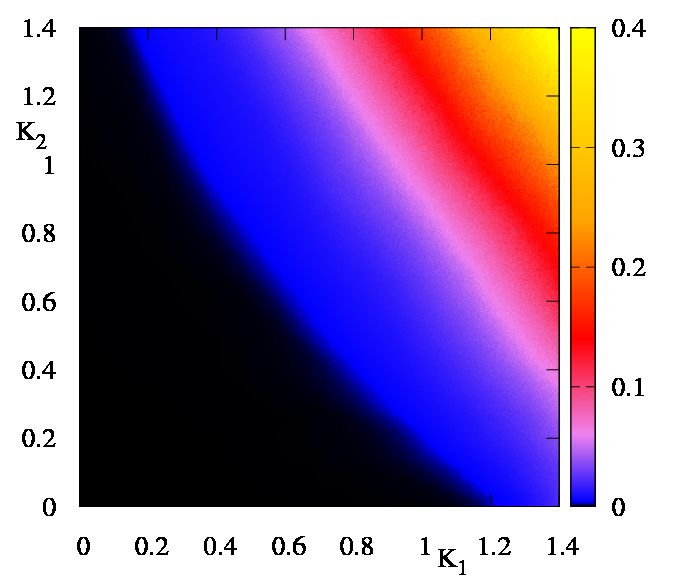
Figure 1: Diffusion rate in momentum $D=\langle p^{2}\rangle/t$ vs $K_{1}$ and $K_{2}$. Data are averaged over $1000$ trajectories with random initial conditions in the interval $x,p\in[0,10^{-6})$ for the number of iterations $t=10^{4}$. Color bar shows the values of $D$.

To study the properties of classical dynamics of map (4) we lunch a bunch of trajectories in a vicinity of unstable fixed point $x=0,p=0$ and compute an effective diffusion coefficient $D=<p^{2}>/t$ averaged over all initial trajectories. The dependence of $D$ on $K_{1}$ and $K_{2}$ is shown in Fig. 1. These data show that there is a critical curve $K_{c2}=f(K_{c1})$ below which the momentum oscillations ave bounded and above which $p$ grows diffusely with time. At $K_{1}=K_{2}=K$ we obtain $K_{c}=K_{c1}=K_{c2}\approx 0.65$ (see below). Of course, the time $t$ used in Fig. 1 is not very large (due to many trajectories and many $K_{1},K_{2}$ values) so that we obtain only an approximate position of the critical curve. Thus for $K_{2}=0$ we know that $K_{c}=0.9716...$ mackay that is a bit below than the blue domain with a finite diffusion rate $D$. This happens due to not very large $t=10^{4}$ value and a small diffusion near $K_{c}$ being $D\approx 0.3(K-K_{c})^{3}$ for the map (1) chirikov ; dls1987 .

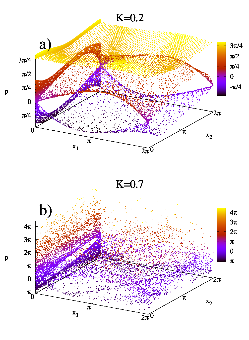
Figure 2: Poincaré section in the phase space $(x_{1},x_{2},p)$ for $K=K_{1}=K_{2}=0.2$ (a) and $K=K_{1}=K_{2}=0.7$ (b). a)The data are obtained from two trajectories with $t=5000$ map iterations for the initial values $p=x_{1}=0.01,x_{2}=0.01\times\nu$ with $p=0.01$ and $p=\pi/\sqrt{2}$; b)the initial phases $x_{1},x_{2}$ are the same as in (a) and $p=0.01$. Color bars show $p$ values.

To represent trajectories on the Poincaré section it is convenient to use variables $x_{1}=x(\mod 2\pi)$, $x_{2}=\alpha x(\mod 2\pi)$ and $p$. We show two sections for $K=K_{1}=K_{2}$ below the critical value at $K=0.2<K_{c}$ and above the critical value at $K=0.7>K_{c}$ (see Fig. 2). For $K=0.2$ there are smooth invariant KAM surfaces bounding $p$ variations while for $K=0.7$ there is a chaotic unbounded dynamics in momentum.

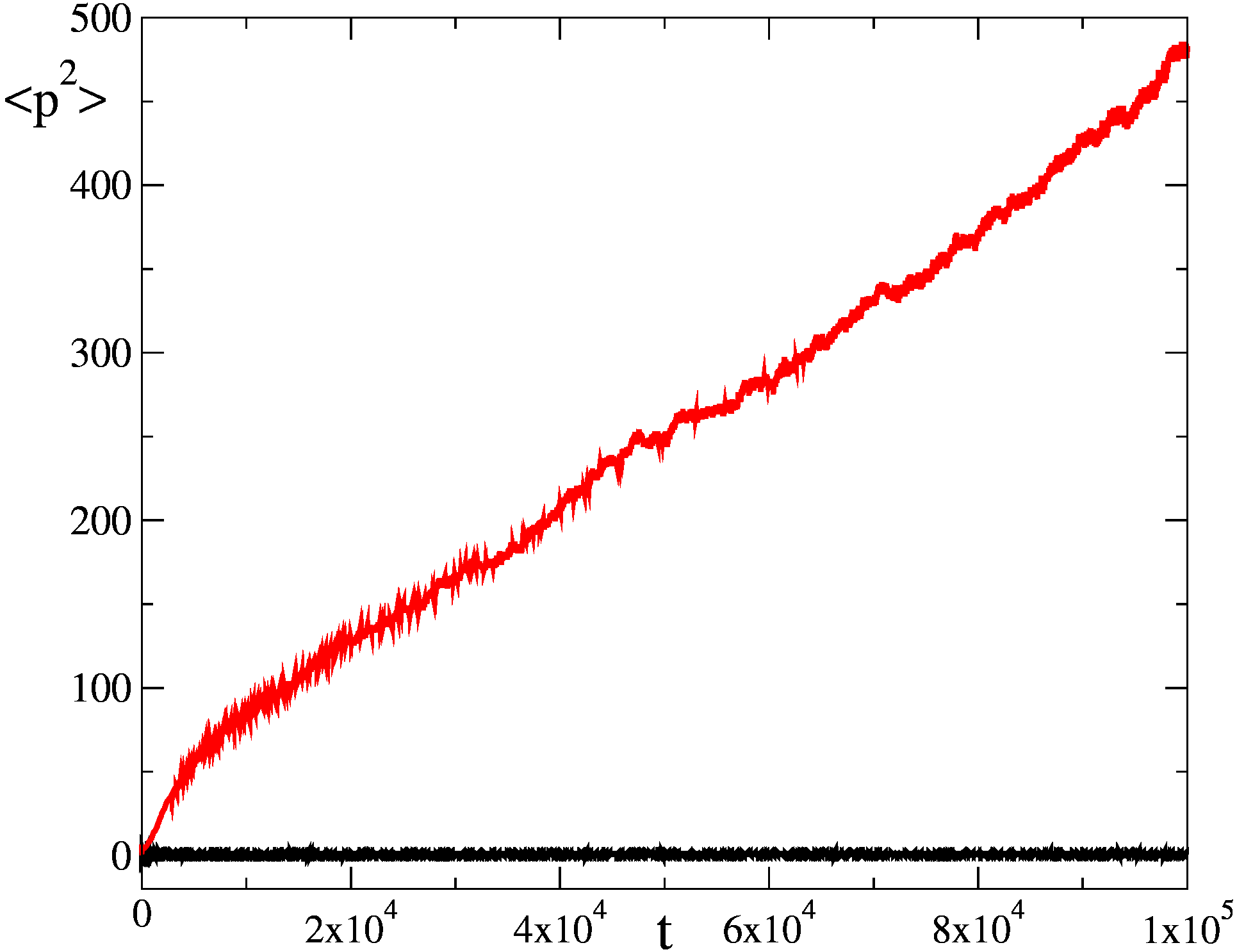
Figure 3: Dependence of $\langle p^{2}\rangle$ on time $t$ for $K_{1}=K_{2}=0.2$ in black (bottom) and $K_{1}=K_{2}=0.7$ in red (top) solid curves. The average is done over $1000$ trajectories with random initial conditions in the range $x,p\in[0,10^{-6})$ (similar to initial conditions as in Fig. 1).

When the last KAM surface is destroyed we have a diffusive growth of momentum as it is shown in Fig. 3 for $K=K_{1}=K_{2}=0.7>K_{c}$. For $K=K_{1}=K_{2}=0.2<K_{c}$ the values of $p$ remain bounded for all times.

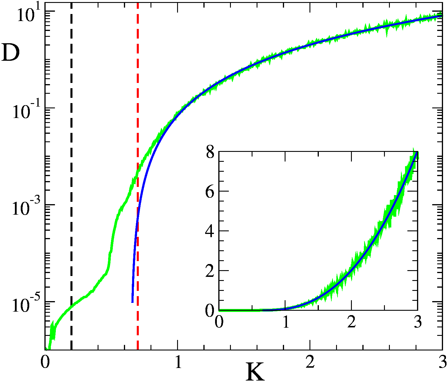
Figure 4: Dependence of diffusion rate $D=\langle p\rangle/t$ on $K=K_{1}=K_{2}$ shown by green (gray) curve, where vertical black and red (gray) dashed lines mark values $K=K_{1}=K_{2}=0.2$ and $K=K_{1}=K_{2}=0.7$ respectively. The fit dependence $D=D_{0}(K-K_{c})^{\alpha}$ is shown by blue (black) curve with the fit values $D_{0}=0.95\pm 0.04$, $k_{c}=0.65\pm 0.02$ and $\alpha=2.5\pm 0.03$. Inset plot show the same curve for linear scale in $D$ axis. Data are obtained from $1000$ trajectories and $t=10^{5}$ iterations.

From the time dependence of $\langle p^{2}\rangle$ on time $t$ we compute the diffusion rate $D$. The dependence of $D$ on $K=K_{1}=K_{2}$ is shown in Fig. 4. We find that this dependence is satisfactory described by the relation $D=D_{0}(K-K_{c})^{\alpha}$ with $D_{0}\approx 0.95$, $K_{c}\approx 0.65$ and $\alpha\approx 2.5$. The value of the exponent $\alpha$ is close to the one for the Chirikov standard map with $\alpha\approx 3$ chirikov ; meiss ; dls1987 . Of course, the number of iterations $t=10^{5}$ is not very large and due to that we have only approximate values of the fit parameters $D_{0},K_{c},\alpha$. It is possible that the real value $K_{c}$ is a bit smaller then the it value $K_{c}=0.65$ but more exact determination of these values require separate studies.

With the obtained global properties of the classical $i-$standard map we go to analysis of its quantum evolution in next Sections.

III Quantum map evolution

The quantum evolution of $i$-standard map is described by the following transformation of wave function on one map period:

$$\bar{\psi}=\exp[-i(k_{1}\cos x+(k_{2}/\nu)\cos\nu x)]$$

$$\times\exp[-i{\hat{p}}^{2}/2\hbar]\;\psi\;$$ (5)

with $k_{1}=K_{1}/\hbar$, $k_{2}=K_{2}/\hbar$ and normalization condition ${\int^{\infty}}_{-\infty}|\psi(x)|^{2}dx=1$. Here, the wave function $\psi$ evolution is considered on infinite domain $-\infty<x<\infty$ corresponding to dynamics of cold atoms in kicked optical lattices; the first multiplier describes kick from optical lattice and the second one gives a free propagation in empty space. The kick potential is $V(x)=k_{1}\cos x+(k_{2}/\nu)\cos\nu x$.

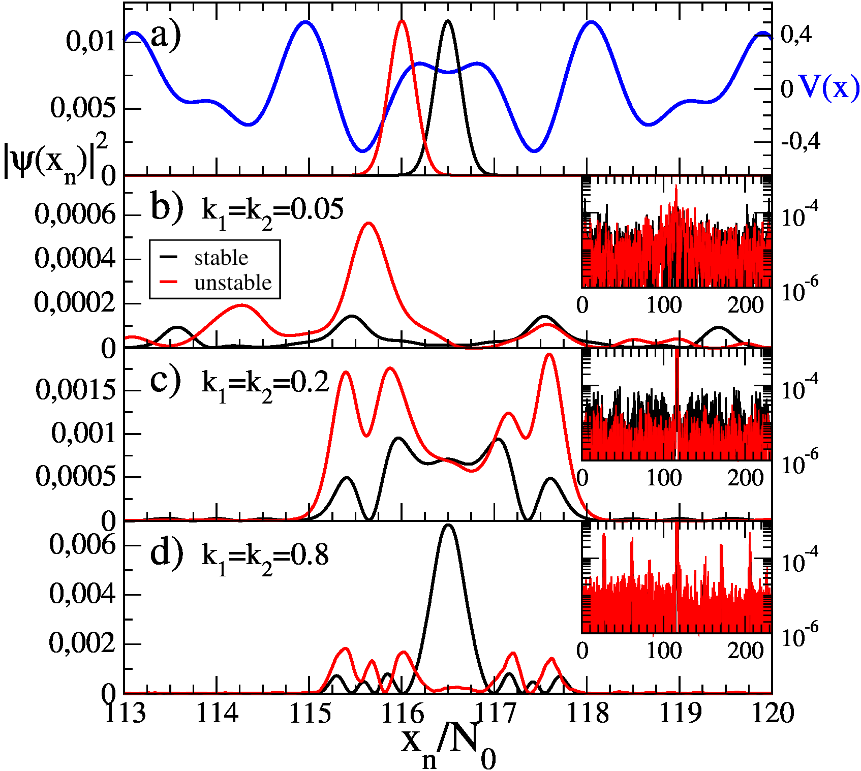
Figure 5: Probability distribution in coordinate. Panel (a) shows the probability distribution in coordinate for initial state given by a Gaussian centered at stable (black curve) and unstable (red/gray curve) conditions. Blue (dark black) curves shows the potential energy $V(x)$ for $k_{1}=k_{2}=0.2$ where the scale is shown in right side. Panels (b), (c), (d) (from top to bottom) show respectively the distributions for $k_{1}=k_{2}=0.05$ $k_{1}=k_{2}=0.2$ and $k_{1}=k_{2}=0.8$ after $t=10^{4}$ iterations with black and red curves showing the cases of stable and unstable initial conditions. In each panel, top-right insets show the same distribution in logarithmic scale and for the whole Hilbert space. In all cases $T=76\pi/3^{5}\approx 0.983$.

To perform numerical simulations of the quantum map (5) we approximate $\nu$ by its Fibonacci series with $\nu_{m}=r_{m}/q_{m}=144/233$ considering time evolution on a ring of size $[0,2\pi q_{m})$ with periodic boundary conditions. Here $r_{m}=f_{m-1}$ and $q_{m}=f_{m}$, are the $(m-1)^{\text{th}}$ and $m^{\text{th}}$ Fibbonaci numbers given by $f_{m}=f_{m-1}+f_{m-2}$ with $f_{1}=f_{2}=1$, and therefore $\lim_{m\rightarrow\infty}\nu_{m}=\nu$. Then one iteration of the map is obtained as

$$\bar{\psi}={\hat{F}^{-1}}e^{-i\left[k_{1}\cos{\left(\frac{2\pi x_{n}}{N_{0}}\right)}+\frac{k_{2}}{\nu_{m}}\cos{\left(\frac{2\pi\nu_{m}x_{n}}{N_{0}}\right)}\right]}{\hat{F}}e^{-i\frac{T}{2}(\frac{p_{n}}{q_{m}})^{2}}\psi$$ (6)

where $T=\hbar$ and the Hilbert space dimension is $N=N_{0}\times q_{m}$, with $q_{m}$ ($r_{m}$) periodic space cells of internal dimension $N_{0}$ for $k_{1}$ ($k_{2}$) harmonic of $V(x)$. Here positions and momentum have integer values $x_{n}=n$ and $p_{n}=(n-\lfloor N/2\rfloor)$ with $n=0,\ldots,N-1$; and ${\hat{F}}$ and ${\hat{F}^{-1}}$ are the operators of discrete Fourier transform from momentum to coordinate representation and back. For numerical simulations we have chosen $N_{0}=3^{5}=243$, $r_{m}=144$ and $q_{m}=233$, with $\hbar=\frac{76\pi}{3^{5}}\simeq 0.983$.

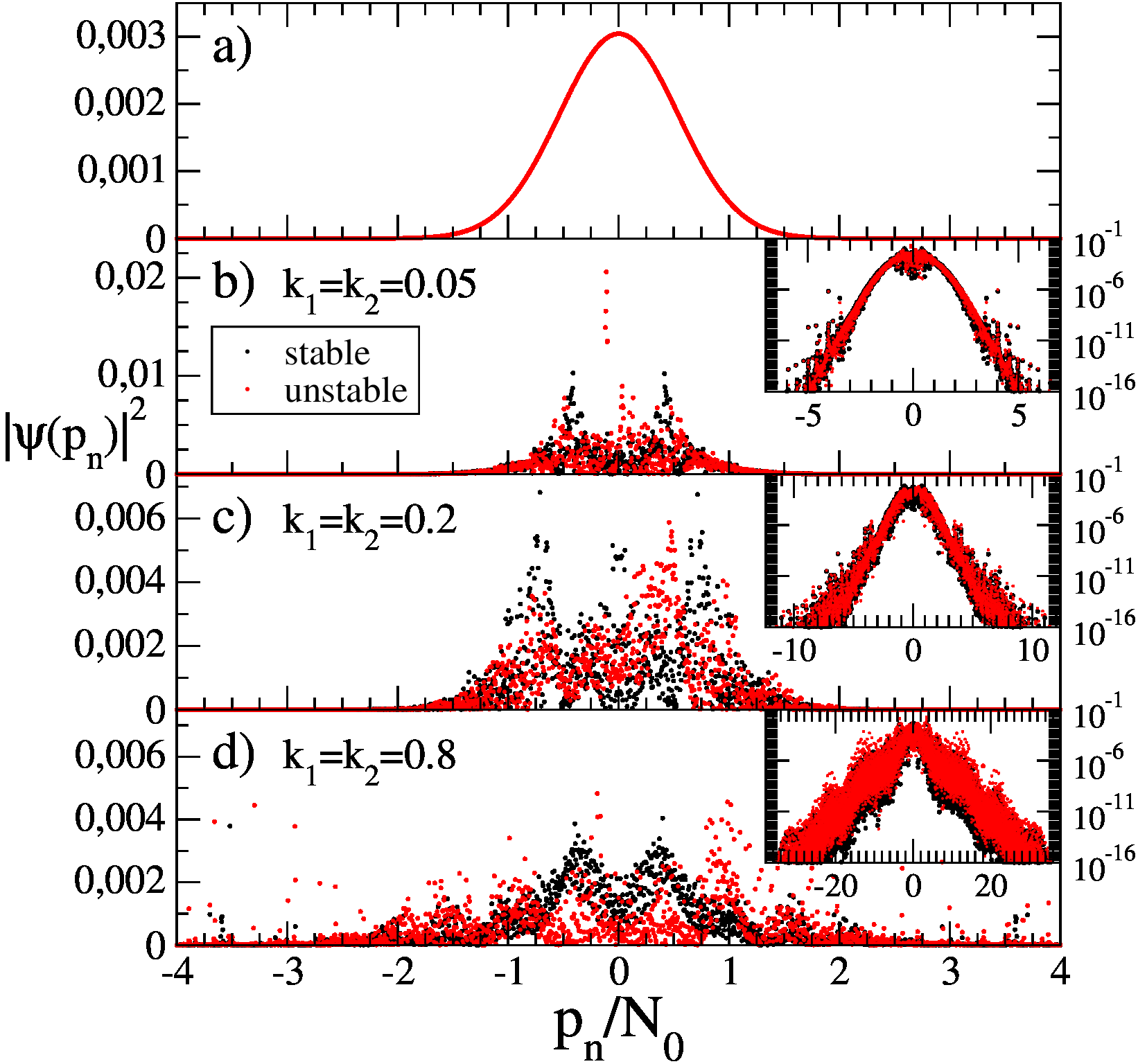
Figure 6: Probability distribution in momentum for the same cases than 5. Top panel show the probability distribution in momentum for initial state given by a Gaussian centered at zero (the same for stable and unstable conditions). In second, third and fourth panels (from top to bottom) the distribution is shown for $k_{1}=k_{2}=0.05$, $k_{1}=k_{2}=0.2$ and $k_{1}=k_{2}=0.8$ after $t=10^{4}$ iterations where black and red dots illustrate the cases of stable and unstable conditions. In each panel, top-right insets show the same distribution in logarithmic scale and for the whole Hilbert space. In all cases $T=76\pi/3^{5}\approx 0.983$.

We choose as an initial configuration a Gaussian wave packet centered at stable (or unstable) point of the kick potential $V(x)=k_{1}\cos{x}+(k_{2}/\nu)\cos{\nu x}$. On a discrete lattice of $x_{n}=n$ ($0\leq n<N$) this distribution is $\psi(x_{n})=A\exp[-(x_{n}-X_{0})^{2}/(2(N_{0}/5))^{2})]$ with $\langle x\rangle=X_{0}$ and $A$ a normalization factor. The corresponding distribution, in momentum space $p_{n}$, is obtained by the discrete Fourier transform, where in this case $\langle p\rangle=P_{0}=0$.

We define $P_{3,x}(t)$ and $P_{3,p}(t)$ as the probability to stay in 3 cells centered at initial $X_{0}$ and $P_{0}$ values respectively:

$$P_{3,x}(t) = \sum_{n=\left\lfloor X_{0}-\frac{3N_{0}}{2}\right\rfloor}^{\left\lfloor X_{0}+\frac{3N_{0}}{2}\right\rfloor}|\psi(x_{n})|^{2}$$ (7)

$$P_{3,p}(t) = \sum_{n=\left\lfloor P_{0}-\frac{3N_{0}}{2}\right\rfloor}^{\left\lfloor P_{0}+\frac{3N_{0}}{2}\right\rfloor}|\psi(p_{n})|^{2}\$$ (8)

where $\lfloor x\rfloor$ is the integer part of x.

The initial probability distributions placed in a vicinity of stable and unstable fix points of the kick potential $V(x)$ are shown in Fig. 5. We note that for small $k_{1}\sim k_{2}\ll 1$ the map approximately describes a continuous time evolution in a static potential. In modugno it is shown that in this case the quantum evolution is approximately reduced to the Aubry-André model on a discrete lattice with the eigenstates of the stationary Schrödinger equation:

$$\begin{array}[]{c}\lambda\cos(\hbar n+\beta)\phi_{n}+\phi_{n+1}+\phi_{n-1}=E\phi_{n}\;.\end{array}$$ (9)

Here $\lambda$ is an effective dimensional energy of the quasiperiodic potential and the hopping amplitude being unity. A metal-insulator transition (MIT) takes place from localized states at $\lambda>2$ to delocalized eigenstates at $\lambda<2$ aubryandre . A review of the properties of the Aubry-André model can be found in sokoloff and the mathematical prove of MIT is given in lana1 . An estimate obtained in modugno shows that $\lambda\propto k_{2}\exp(-C_{1}/{k_{1}}^{C_{2}}+2C_{3}\sqrt{k_{1}})$ for an irrational $\nu\sim 1$ with $C_{1},C_{2},C_{3}$ being numerical constants order of unity. This approximate reduction of the Schrödinger equation in a continuous quasiperiodic potential $V(x)$ to the discrete lattice Aubry-André model have been used in experiments with cold atoms where the MIT was found at $\lambda=2$ inguscio ; bloch .

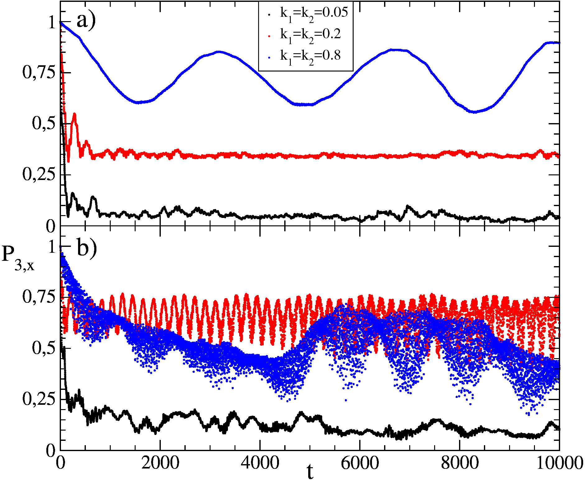
Figure 7: Time evolution of the probability to stay in the first 3 space cells $P_{3,x}$ for the cases of Figs 5 and 6 with $N_{0}=243$ and $q_{m}=233$. Top (a) and bottom (b) panels show the stable and unstable conditions of Fig. 5 respectively for $k_{1}=k_{2}=0.05$ (black circles), $k_{1}=k_{2}=0.2$ (red circles) and $k_{1}=k_{2}=0.8$ (blue circles) ordered from bottom to top in each panel.

The signs of MIT are visible in Fig. 5 with a delocalization of probability in space at $k_{1}=k_{2}=0.05$ and localization at $k_{1}=k_{2}=0.2;0.8$. At the same time the results of Fig. 6 show that the probability distribution in momentum remains exponentially localized for the above $k_{1},k_{2}$ values.

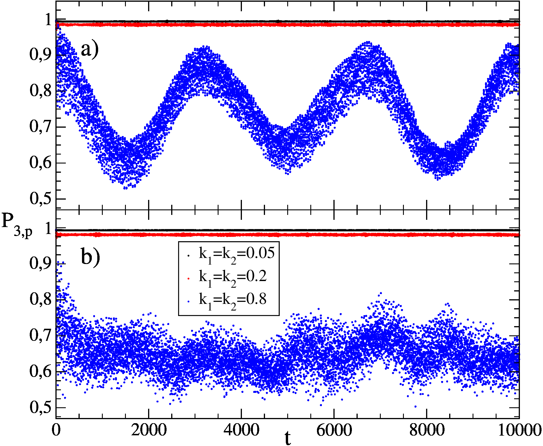
Figure 8: Time evolution of the probability to stay in the first 3 momentum cells $P_{3,p}$ for the cases of Figs 5 and 6 with $N_{0}=243$ and $q_{m}=233$. Top (a) and bottom (b) panels show the stable and unstable conditions of Fig. 6 respectively for $k_{1}=k_{2}=0.05$ (black circles), $k_{1}=k_{2}=0.2$ (red circles) and $k_{1}=k_{2}=0.8$ (blue circles) ordered from top to bottom in each panel.

The time evolution of probabilities of stay in a vicinity of initial cell $P_{3,x}$ and $P_{3,p}$ are shown in Fig. 7 and Fig. 8. We see that at $k_{1}=k_{2}=0.05$ only a small fraction of probability (about 10 percent) remains in a vicinity of initial space cell while in contrast it is rather large for $k_{1}=k_{2}=0.2;0.8$. In contrast for the distribution in momentum about 99 percent remains in a vicinity of initial cell for $k_{1}=k_{2}=0.05;0.2$ and 65 percent for $k_{1}=k_{2}=0.8$. Thus this data confirms localization in momentum and MIT transition is space similar to the MIT discussed in modugno in the limit of energy conservative system corresponding to the dynamics of our kicked model at small $k_{1},k_{2}$ values.

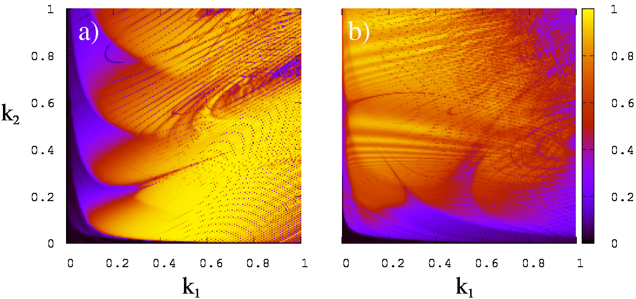
Figure 9: Probability $P_{3,x}(t)$ averaged in time within interval $t\in(9000,10000]$ is shown as a function of $k_{1}$ and $k_{2}$. Here $T=0.983...$ and the initial condition is centered at stable and unstable points of the potential in (a) and (b) panels respectively.

The global dependence of probabilities $P_{3,x}(t)$ and $P_{3,p}(t)$ on kick amplitudes $k_{1},k_{2}$ are shown in Figs. 9,10 for initial packet centered in a vicinity of stable or unstable point. For $P_{3,x}(t)$ there is a clear region on $k_{1},k_{2}$-plane where the probability $P_{3,x}(t)$ drops significantly corresponding to delocalization in space (see Fig. 9)). In contrast, the probability $P_{3,p}(t)$ remains always rather high showing that the classical chaotic diffusion in momentum is localized by quantum interference effects.

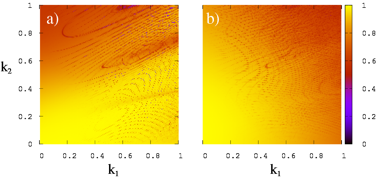
Figure 10: Probability $P_{3,p}(t)$ in momentum averaged in time within interval $t\in(9000,10000]$ is shown as a function of $k_{1}$ and $k_{2}$. Here $T=0.983...$ and the initial condition is centered at stable and unstable points of the potential in left (a) and right (b) panels respectively.

In Fig. 11 we consider a case with a smaller value of $T=0.2$ so that the system becomes more close to the case of stationary potential analyzed in modugno . This data are similar to the case at larger $T=0.983...$ with a domain of small probability $P_{3,x}(t)$ values at small $k_{1},k_{2}$ indicated the delocalization of probability in space. At the same time the probability $P_{3,p}(t)$ in momentum remains always localized.

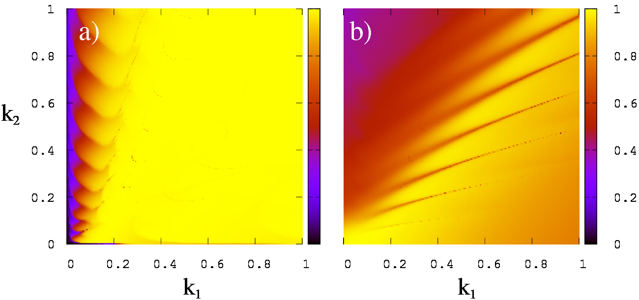
Figure 11: Probability $P_{3,x}(t)$ in space (a) and $P_{3,p}(t)$ in momentum (b) averaged in time within interval $t\in(9000,10000]$ are shown as a function of $k_{1}$ and $k_{2}$. The initial condition in $x$ is centered at stable points of the potential and $T=0.2$.

The obtained results show the presence of certain space delocalization of the quantum incommensurate map at small kick amplitudes while at large amplitudes the probability remains localized. The probability in momentum remains localized for all $k_{1},k_{2}$ values at irrational $T/2\pi$ values.

At the same time we note that the rigorous prove of probability delocalization in our model remains a mathematical challenge since the map of our system (or even its stationary version considered in modugno ) on the Aubry-André model (9) works only approximately. Indeed, in our model it is possible to have excitation of high energy states (even if the numerical results indicate localization in momentum) that complicates the dynamics. We hope that the skillful mathematical tools developed in lana1 will allow to obtain mathematical results for the quantum incommensurate standard map.

Below we consider the localization properties in momentum in more detail.

IV 2D and 3D models of i-standard map

To analyze the localization properties in momentum we note that the kick with $k_{1}$ generates integer harmonics of $\exp(-ij_{i}x)$ while the kick with $k_{2}$ generates only harmonics $\exp(-ij_{2}\nu x)$ with integer $j_{1},j_{2}$ values. Due to that the wave function contains only these two types of harmonics and the system evolution is described by

$$\bar{\psi}={\hat{F}^{-1}}e^{-i[k_{1}\cos{x}+k_{2}\cos{\nu x}]}{\hat{F}}e^{-iT(j_{1}+\nu j_{2})^{2}/2}\psi\;,$$ (10)

where ${\hat{F}}$ is the 2D-fast Fourier transformation from momentum to space representation and ${\hat{F}^{-1}}$ gives a back transformation from space to momentum. The integers $j_{1}$ and $j_{2}$ number the correspondent harmonic numbers with the energy phase of free propagation between kicks being $\phi_{E}=Tp^{2}/2=T(j_{1}+\nu j_{2})^{2}/2$ with $p=(j_{1}+\nu j_{2})$. If we would have $\phi_{E}(j_{1},j_{2})$ taking random values for each $j_{1},j_{2}$ then we would have 2D kicked rotator with the Anderson type localization in 2D. In such a case we would expect that the localization length $\lambda$ grows exponentially with the diffusion rate $\ln\lambda\sim D\sim({k_{1}}^{2}+{k_{2}}^{2})/2$ (see e.g. dls1987 ; borgonovi ; imry ). However, the phases $\phi_{E}(j_{1},j_{2})$ are not random but incommensurate and the appearance of 2D Anderson localization is not so obvious.

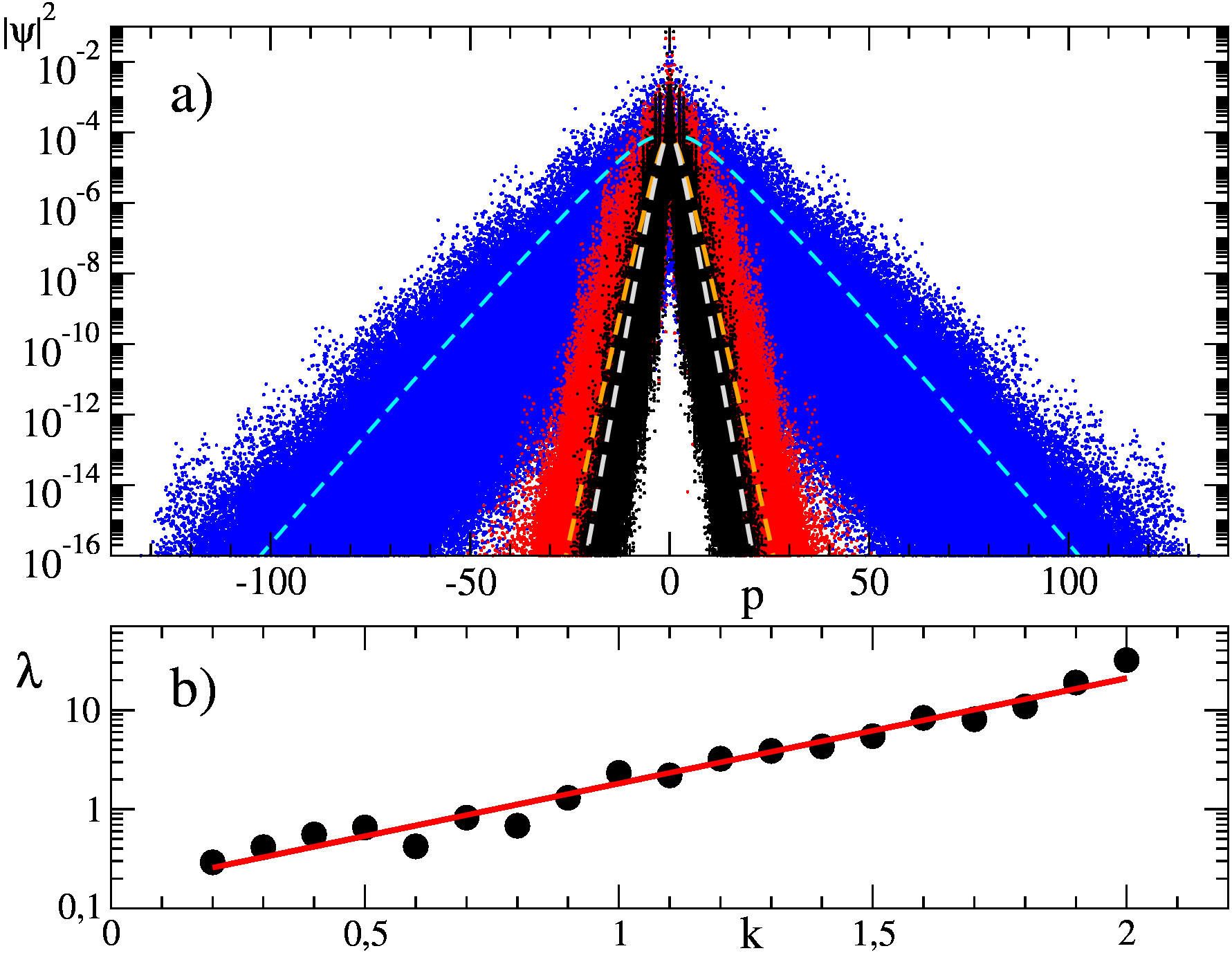
Figure 12: (a) Probability distribution $|\psi(j_{1},j_{2})|^{2}$ in the model (10) as a function of $p=j_{1}+\nu j_{2}$ shown at time $t=10^{4}$. Here $T=2$ and $N_{2}=3^{7}=2187$ ($N=4782969$). Black (internal domain), red/gray (middle domain) and blue/dark (external domain) circles represent $k=k_{1}=k_{2}=0.5,0.7,1.2$ respectively. Numerical fits of $|\psi|^{2}\sim e^{-\frac{p}{\lambda}}$ with localization length values are shown by dashes lines with $\lambda{(k=0.5)}\approx 0.656$, $\lambda{(k=0.7)}\approx 0.822$ and $\lambda{(k=1.2)}\approx 3.22$. Panel (b) shows the exponential dependence of fitted values of $\lambda$ as a function of $k$. Numerical fit is shown by the straight line with the exponential growth $\lambda\approx 0.16\exp{(2.44k)}$. Initial state is at $j_{1}=j_{2}=0$.

For investigation of this expected 2D localization we take $N_{2}=3^{7}$ harmonics $j_{1}$ and $j_{2}$ so that the total number of states becomes $N={N_{2}}^{2}=4782969$. The results of numerical show an exponential decay of probability with momentum $p$ as it is shown in Fig. 12(a) for a few $k=k_{1}=k_{2}$ values. We fit this decay by an exponential dependence $|\psi(p)|^{2}\sim\exp(-|p|/\lambda)$ thus determining the localization length $\lambda$. The results presented in Fig. 12(b). show the expected exponential growth of localization length $\ln\lambda\sim 2.3k$. The fact that $\ln\lambda$ is proportional to $k$ and not to expected $k^{2}$ can be attributed to the fact that we are still relatively close to the chaos border (see Fig. 4) and that the diffusion rate is small while the estimate $\ln\lambda\sim D\sim k^{2}$ assumes well developed chaotic regime with a relatively high $D$ imry .

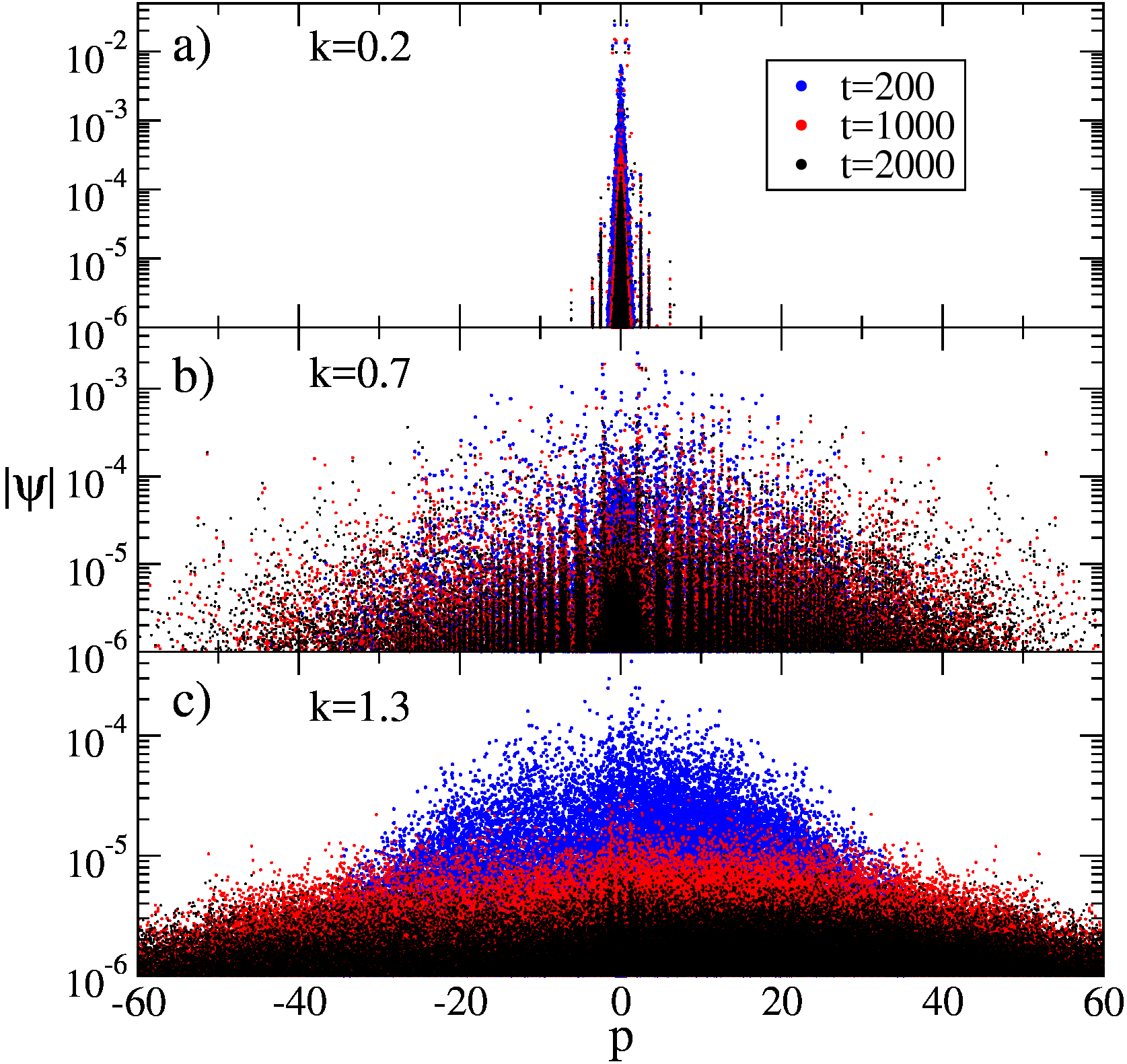
Figure 13: Probability distribution $|\psi(j_{1},j_{2},j_{3})|^{2}$ in the model (11) as a function of $p=j_{1}+j_{2}/\theta+j_{3}/\theta^{2}$ where $\theta$ is the solution of $\theta^{3}-\theta-1=0$. Here $T=2$ and $N_{3}=529$ ($N={N_{3}}^{3}=148035889$) at evolution times $t=200,1000,000$ with blue (top dark points), red (middle gray points) and black (bottom) points respectively. Top (a), middle (b) and bottom (c) panels show the cases of $k_{1}=k_{2}=k_{3}=0.2$, $k_{1}=k_{2}=k_{3}=0.7$ and $k_{1}=k_{2}=k_{3}=1.3$. Initial state is at $j_{1}=j_{2}=j_{3}=0$. The Anderson transition takes place at $k=k_{1}=k_{2}\approx 0.7$.

There is no delocalization in 2D but in 3D there is the Anderson transition to delocalization anderson if a disorder is below a critical value or chaotic diffusion rate is higher a certain border (see e.g. imry ). We argue that 3D case can be realized in our model if we add kick with one more incommensurate potential $V_{3}(x)=k_{3}\cos\nu_{3}x$. Then the wave function additional harmonics $\exp(-ij_{3}\nu_{3}x)$ and in analogy with (10) the time evolution is described by

$$\bar{\psi} = {\hat{F}^{-1}}e^{-i[k_{1}\cos{x}+k_{2}\cos{\nu x}+k_{3}\cos{\nu_{3}x]}}$$ (11)

$$\times {\hat{F}}e^{-iT(j_{1}+\nu j_{2}+\nu_{3}j_{3})^{2}/2}\psi\;,$$

where momentum integer harmonics are $j_{1},j_{2},j_{3}=1,...,N_{3}$ and with the total dimension $N=N_{3}^{3}=529^{3}=148035889$ and $p=j_{1}+j_{2}/\theta+j_{3}/\theta^{2}$, with irrational $\theta=1.32471795724475...$ being the solution of equation $\theta^{3}-\theta-1=0$. Thus $\nu=1/\theta$, $\nu_{3}=1/\theta^{2}$.

The results for time evolution of probability are presented in Fig. 13. They clearly show that at $k=k_{1}=k_{2}=0.2$ there is exponential Anderson localization of probability over momentum anderson . For $k=k_{1}=k_{2}=1.3$ there is spreading of probability in time over momentum states. The case at $k=k_{1}=k_{2}=0.7$ is close to a critical parameter value where the Anderson transition takes place. Thus the MIT point is located in the range $0.7\leq k_{c}<1.3$. Additional studies should be performed to obtain the critical parameter more exactly but the presented results definitely show that the transition takes place for $k$-parameter in this range.

V Discussion

In our research we determined the main properties of the incommensurate standard map for its classical dynamics and for its quantum evolution. In the classical case the invariant KAM surfaces are destroyed above certain kick amplitudes given us a critical curve on the plane of kick amplitudes $K_{1},K_{2}$ (see Fig. 1). We find that above the critical curve at its vicinity the diffusion rate is characterized by a critical exponent $\alpha\approx 2.5$ which is not so far from the case of the Chirikov standard map.

The quantum evolution at small quantum kick amplitudes $k_{1}=K_{1}/\hbar$, $k_{2}=K_{2}/\hbar$ is similar to the Aubry-André type transition aubryandre as discussed in modugno and observed in cold atom experiments with a static incommensurate potential inguscio ; bloch . However, at larger values of $k_{1},k_{2}$ the evolution remain localized both in space and momentum. We show that the localization in momentum is similar to the case of Anderson localization in 2D. While a significant progress has been reached with rigorous results for Aubry-André model lana1 , we point that the mathematical prove of space and momentum localization for the quantum incommensurate standard map represents a high challenge for mathematicians.

The quantum evolution for the quantum $i-$standard map is always localized in momentum, as in the case of 2D Anderson localization. However, for three kick-harmonics the situation becomes similar to the 3D Anderson localization with MIT from localized to delocalized evolution as the kick amplitude is increased. We note that this behavior has similarities with the frequency modulated kicked rotator introduced in dls1983 which also demonstrates the Anderson localization in effective 2 and 3 dimensions borgonovi observed in the cold atoms experiments garreau ; garreau2 . Thus the kicked rotator with one additional modulation frequency in time domain is similar to the case of 2D Anderson localization in agreement with predictions done in 1983 dls1983 . The case of 2 additional modulation frequencies is similar to the case of 3D Anderson transition as discussed in borgonovi . We hope that the results presented here will allow to investigate the Anderson localization in 2D and 3D for periodically kicked rotator with kicked incommensurate potential discussed in this work.

As it was pointed in Section I the incommensurate standard map naturally appears for a description of dynamics of dark matter or comets in the Solar System and other planetary systems with 2 or more planets rotating around the central star. Recently it has been shown that in the case of star and one rotating planet the quantum effects can play a significant role for escape of very light dark matter from the planetary system due to the Anderson localization of energy transitions dlsdmp . The obtained results show that a presence of second planet leads to the dynamics described by the incommensurate standard map with significant effects on the quantum localization of dark matter.

Since the Chirikov standard map has many universal features and appears in the description of evolution of many very different physical systems we argue that the incommensurate standard map will also find a broad field of applications.

VI Acknowledgments

This work was supported in part by the Programme Investissements d’Avenir ANR-11-IDEX-0002-02, reference ANR-10-LABX-0037-NEXT (project THETRACOM). This work was granted access to the HPC resources of CALMIP (Toulouse) under the allocation 2018-P0110.

References

- eprint
- (1) H. Poincaré, Sur le problème des trois corps et les équations de la dynamique, Acta Math. 13, 1 (1890).
- (2) V.I. Arnold and A. Avez, Ergodic problems of classical mechanics, (Benjamin, Paris, 1968).
- (3) I.P. Cornfeld, S.V. Fomin, and Y.G. Sinai, Ergodic theory, (Springer, New York, 1982).
- (4) B. V. Chirikov, A universal instability of many-dimensional oscillator systems , Phys. Rep. 52, 263 (1979).
- (5) A.J. Lichtenberg, M.A. Lieberman, Regular and chaotic dynamics, (Springer, Berlin, 1992).
- (6) R.S. MacKay, A renormalisation approach to invariant circles in area-preserving maps, Physica D 7, 283 (1983).
- (7) J.D. Meiss, Symplectic maps, variational principles, and transport, Rev. Mod. Phys. 64(3), 795 (1992).
- (8) B. Chirikov and D. Shepelyansky, Chirikov standard map, Scholarpedia 3(3), 3550 (2008).
- (9) M. Raizen, and D.A. Steck, Cold atom experiments in quantum chaos, Scholarpedia 6(11), 10468 (2011).
- (10) D. Shepelyansky, Microwave ionization of hydrogen atoms, Scholarpedia 7(1), 9795 (2012).
- (11) J. Lages, D. Shepelyansky, and I.I. Shevchenko, Kepler map, Scholarpedia 13(2), 33238 (2018).
- (12) B.V. Chirikov, F.M. Izrailev and D.L. Shepelyansky, Dynamical stochasticity in classical and quantum mechanics, Mathematical physics reviews (Sov. Scient. Rev. C - Mathematical Physics Reviews, Ed. S.P.Novikov) 2, 209 (1981).
- (13) B.V. Chirikov, F.M. Izrailev and D.L. Shepelyansky, Quantum chaos: localization vs. ergodicity, Physica D 33, 77 (1988).
- (14) F.L. Moore, J.C. Robinson, C.F. Bharucha, B. Sundaram, and M.G. Raizen, Atom optics realization of the quantum -kicked rotor, Phys. Rev. Lett. 75, 4598 (1995).
- (15) D.L. Shepelyansky, Localization of diffusive excitation in multi-level systems, Physica D 28, 103 (1987).
- (16) S. Fishman, D.R. Grempel, and R.E. Prange, Chaos, quantum recurrences and Anderson localization, Phys. Rev. Lett. 49, 509 (1982).
- (17) S. Fishman, Anderson localization and quantum chaos maps, Scholarpedia 5(8) 9816 (2010).
- (18) K.M. Frahm, adn D.L. Shepelyansky, Diffusion and localization for the Chirikov typical map, Phys. Rev. E 80, 016210 (2009).
- (19) B.V. Chirikov, and V.V. Vecheslavov Chaotic dynamics of comet Halley, Astron. Astrophys. 221, 146 (1989).
- (20) G. Roati, C. D’Errico, L. Fallani, M. Fattori, C. Fort, M. Zaccanti, G. Modugno, M. Modugno, and M. Inguscio, Anderson localization of a non-interacting Bose-Einstein condensate, Nature 453, 895 (2008).
- (21) M. Modugno, Exponential localization in one-dimensional quasi-periodic optical lattices, New J. Phys. 11, 033023 (2009).
- (22) S. Aubry, and G. André, Analyticity breaking and Anderson localization in incommensurate lattices, Ann. Israel Phys. Soc. 3, 18 (1980).
- (23) M. Schreiber, S.S. Hodgman, P. Bordia, H.P. Luschen, M.H. Fischer, R. Vosk, E. Altman, U. Schmeider, and I. Bloch, Observation of many-body localization of interacting fermions in a quasirandom optical lattice, Science 349, 842 (2015).
- (24) J.B. Sokoloff, Unusual band structure, wave functions and electrical conductance in crystals with incommensurate periodic potentials, Phys. Rep. 126(4), 189 (1985).
- (25) S. Jitomirskaya, Metal-insulator transition for the almost Mathieu operator, Ann. Math. 150(3), 1159 (1999).
- (26) F. Borgonovi, D.L. Shepelyansky, Two interacting particles in an effective 2-3-d random potential, J. de Physique I France 6, 287 (1996)
- (27) Y. Imry, Introduction to mesoscopic physics, Oxford Univ. Press, Oxford UK (2002).
- (28) P. W. Anderson, Absence of diffusion in certain random lattices, Phys. Rev. 109, 1492 (1958).
- (29) D.L. Shepelyansky, Some statistical properties of simple classically stochastic quantum systems, Physica D 8, 208 (1983).
- (30) J. Chabe, G. Lemarie, R. Cremaud, D. Delande, P. Szriftgiser, and J.C. Garreau, Experimental observation of the Anderson metal-insulator transition with atomic matter waves, Phys. Rev. Lett. 101, 255702 (2008).
- (31) I. Manai, J.-F. Clement, R. Chicireanu, C. Hainaut, J.C. Garreau, P. Szriftgiser, and D. Delande, Experimental observation of two-dimensional Anderson localization with the atomic kicked rotor, Phys. Rev. Lett. 115, 240603 (2015).
- (32) D.L. Shepelyansky, Quantum chaos of dark matter in the Solar system , arXiv:1711.07815 [quant-ph] (2017).