Heat and Moisture Budget Analysis
with an Improved Form of Moist Thermodynamics

Abstract

In order to understand the effects of cumulus convection on large-scale atmospheric motions, heat and moisture budget analyses are often performed using data from an array of radiosonde stations. Ever since the pioneering work of Yanai et al. (1973), such budgets have been based on approximate forms of moist thermodynamics. This paper presents an improved form of moist thermodynamics for such budget studies.

1 Introduction

Ever since the pioneering work of Yanai et al. (1973), heat and moisture budget studies, and their interpretation in terms of the convective flux of moist static energy, have been performed with approximate forms of moist thermodynamics. For example, such studies often begin with the assumption that moist static energy $h=c_{pa}T+gz+Lq$, defined with the latent heat of condensation $L$ assumed constant, is materially conserved (except for radiative effects). This misses important physical effects of ice, such as the formation of stable layers near the melting level. This is only one of several consequences of using this approximate form of moist thermodynamics. While the effects of approximate moist thermodynamics are generally small at a given time, their accumulated effects over longer periods can be substantial. This was apparent to Johnson and Ciesielski (2000) in computing long-term averaged budget residuals such as precipitation and column average radiation for TOGA COARE.

Since its introduction in the late 1990s, the constrained variational analysis (CVA) approach to atmospheric budgets has proved to be an invaluable tool for computing accurate large-scale forcing fields from sounding data networks (Zhang and Lin 1997). In this method the atmospheric state variables, typically derived from sounding data, are adjusted in a minimal way comparable to measurement uncertainty to conserve vertical constraints of mass, moisture, static energy and momentum. In so doing, CVA produces fields that are consistent with these constraints. These additional constraints result in significant improvements in budget diagnostics especially during periods when the original sounding data are missing or of questionable quality. While the effects of measurement and sampling errors in sounding data (Mapes et al. 2003) are effectively minimized with CVA, accurate large-scale diagnostics in this method are dependent on reliable constraints, particularly rainfall (Xie et al. 2004).

Ooyama (1990, 2001) proposed a very accurate form of moist thermodynamics for use in tropical models. This accurate formulation of moist thermodynamics is not limited to modeling studies but can also be used in heat and moisture budget studies. With the advent of GPS sondes and the recent availability of certain satellite data products, this more accurate treatment of moist thermodynamics provides opportunities to refine our understanding of tropical systems. This paper develops more accurate methods, which can utilize ancillary ground-based measurements and satellite data products, for the diagnosis of heat and moisture budgets. The overall goal of this diagnostic technique development is to provide the observational analysis community with an improved method for computing atmospheric budgets, which has the additional advantage of having a complementary numerical modeling framework with the same moist thermodynamics. This should allow better comparisons between satellite latent heating products and numerical model simulations.

2 Review of the standard theoretical basis for heat and moisture budget studies

In the standard theory (Yanai et al. 1973), mass conservation relations are written for only two forms of matter: dry air and water vapor. In addition, a thermodynamic relation for the dry static energy is included. Let $\rho_{a}$ denote the mass density of dry air, $\rho_{v}$ the mass density of water vapor, and $s=c_{pa}T+gz$ the dry static energy. The flux forms of the prognostic equations for $\rho_{a}$, $s$, and $\rho_{v}$ are given by

$$\frac{\partial\rho_{a}}{\partial t}+\frac{\partial(\rho_{a}u)}{\partial x}+\frac{\partial(\rho_{a}v)}{\partial y}+\frac{\partial(\rho_{a}w)}{\partial z}=0,$$ (1)

$$\frac{\partial(\rho_{a}s)}{\partial t}+\frac{\partial(\rho_{a}us)}{\partial x}+\frac{\partial(\rho_{a}vs)}{\partial y}+\frac{\partial(\rho_{a}ws)}{\partial z}=L\rho_{a}(c-e)+\rho_{a}Q_{R},$$ (2)

$$\frac{\partial\rho_{v}}{\partial t}+\frac{\partial(\rho_{v}u)}{\partial x}+\frac{\partial(\rho_{v}v)}{\partial y}+\frac{\partial(\rho_{v}w)}{\partial z}=-\rho_{a}(c-e),$$ (3)

where $c$ is the rate of condensation, $e$ the rate of evaporation, and $Q_{R}$ the radiative heating rate. In the standard theory, the latent heat of condensation $L$ is usually taken to be a constant, in contrast to the more accurate treatment discussed in section 3. Instead of working with the mass density of water vapor, $\rho_{v}$, the standard theory usually works with the water vapor mixing ratio $q_{v}$, which is related to the water vapor mass density by $\rho_{v}=\rho_{a}q_{v}$. The equation for $q_{v}$ is obtained by simply replacing $\rho_{v}$ by $\rho_{a}q_{v}$ everywhere in (3).

Taking the horizontal average of (1)–(3), we obtain

$$\frac{\partial\bar{\rho}_{a}}{\partial t}+\frac{\partial(\overline{\rho_{a}u})}{\partial x}+\frac{\partial(\overline{\rho_{a}v})}{\partial y}+\frac{\partial(\overline{\rho_{a}w})}{\partial z}=0,$$ (4)

$$\frac{\partial(\overline{\rho_{a}s})}{\partial t}+\frac{\partial(\overline{\rho_{a}us})}{\partial x}+\frac{\partial(\overline{\rho_{a}vs})}{\partial y}+\frac{\partial(\overline{\rho_{a}ws})}{\partial z}=L\overline{\rho_{a}(c-e)}+\overline{\rho_{a}Q_{R}},$$ (5)

$$\frac{\partial(\overline{\rho_{a}q_{v}})}{\partial t}+\frac{\partial(\overline{\rho_{a}uq_{v}})}{\partial x}+\frac{\partial(\overline{\rho_{a}vq_{v}})}{\partial y}+\frac{\partial(\overline{\rho_{a}wq_{v}})}{\partial z}=-\overline{\rho_{a}(c-e)}.$$ (6)

Making the usual approximations such as neglecting horizontal eddy flux terms involving $\overline{u^{\prime}s^{\prime}}$, $\overline{v^{\prime}s^{\prime}}$, $\overline{u^{\prime}q_{v}^{\prime}}$, and $\overline{v^{\prime}q_{v}^{\prime}}$, and then making the approximations $\overline{\rho_{a}ws}\approx\bar{\rho}_{a}\bar{w}\bar{s}+\bar{\rho}_{a}\overline{w^{\prime}s^{\prime}}$, and $\overline{\rho_{a}wq_{v}}\approx\bar{\rho}_{a}\bar{w}\bar{q}_{v}+\bar{\rho}_{a}\overline{w^{\prime}q_{v}^{\prime}}$, we can simplify (4)–(6) to

$$\frac{\partial\bar{\rho}_{a}}{\partial t}+\frac{\partial(\bar{\rho}_{a}\bar{u})}{\partial x}+\frac{\partial(\bar{\rho}_{a}\bar{v})}{\partial y}+\frac{\partial(\bar{\rho}_{a}\bar{w})}{\partial z}=0,$$ (7)

$$\frac{\partial(\bar{\rho}_{a}\bar{s})}{\partial t}+\frac{\partial(\bar{\rho}_{a}\bar{u}\bar{s})}{\partial x}+\frac{\partial(\bar{\rho}_{a}\bar{v}\bar{s})}{\partial y}+\frac{\partial(\bar{\rho}_{a}\bar{w}\bar{s})}{\partial z}=-\frac{\partial(\bar{\rho}_{a}\overline{w^{\prime}s^{\prime}})}{\partial z}+L\bar{\rho}_{a}(\bar{c}-\bar{e})+\bar{\rho}_{a}\bar{Q}_{R},$$ (8)

$$\frac{\partial(\bar{\rho}_{a}\bar{q}_{v})}{\partial t}+\frac{\partial(\bar{\rho}_{a}\bar{u}\bar{q}_{v})}{\partial x}+\frac{\partial(\bar{\rho}_{a}\bar{v}\bar{q}_{v})}{\partial y}+\frac{\partial(\bar{\rho}_{a}\bar{w}\bar{q}_{v})}{\partial z}=-\frac{\partial(\bar{\rho}_{a}\overline{w^{\prime}q_{v}^{\prime}})}{\partial z}-\bar{\rho}_{a}(\bar{c}-\bar{e}).$$ (9)

Using (7), the flux forms (8) and (9) can be converted to the advective forms

$$Q_{1}\equiv\frac{\partial\bar{s}}{\partial t}+\bar{u}\frac{\partial\bar{s}}{\partial x}+\bar{v}\frac{\partial\bar{s}}{\partial y}+\bar{w}\frac{\partial\bar{s}}{\partial z}=-\frac{\partial(\bar{\rho}_{a}\overline{w^{\prime}s^{\prime}})}{\bar{\rho}_{a}\partial z}+L(\bar{c}-\bar{e})+\bar{Q}_{R},$$ (10)

$$Q_{2}\equiv-L\left(\frac{\partial\bar{q}_{v}}{\partial t}+\bar{u}\frac{\partial\bar{q}_{v}}{\partial x}+\bar{v}\frac{\partial\bar{q}_{v}}{\partial y}+\bar{w}\frac{\partial\bar{q}_{v}}{\partial z}\right)=L\frac{\partial(\bar{\rho}_{a}\overline{w^{\prime}q_{v}^{\prime}})}{\bar{\rho}_{a}\partial z}+L(\bar{c}-\bar{e}),$$ (11)

with the first equality in (10) serving as the definition of the apparent heat source $Q_{1}$ and the first equality in (11) serving as the definition of the apparent moisture sink $Q_{2}$. If a network of upper air observations gives us $\bar{u}$, $\bar{v}$, $\bar{\rho}_{a}$, $\bar{s}$, and $\bar{q}_{v}$, and if we compute $\bar{w}$ from (7), then we can compute the apparent heat source $Q_{1}$ from the large-scale terms in (10) and the apparent moisture sink $Q_{2}$ from the large-scale terms in (11). Subtracting (11) from (10), we obtain

$$\frac{\partial\bar{h}}{\partial t}+\bar{u}\frac{\partial\bar{h}}{\partial x}+\bar{v}\frac{\partial\bar{h}}{\partial y}+\bar{w}\frac{\partial\bar{h}}{\partial z}-\bar{Q}_{R}=Q_{1}-Q_{2}-\bar{Q}_{R}=-\frac{\partial(\bar{\rho}_{a}\overline{w^{\prime}h^{\prime}})}{\bar{\rho}_{a}\,\partial z},$$ (12)

where $\bar{\rho}_{a}\overline{w^{\prime}h^{\prime}}$ is the vertical eddy flux of moist static energy, with $h$ defined by $h=c_{pa}T+gz+Lq=s+Lq_{v}$. Assuming that $\overline{w^{\prime}h^{\prime}}$ vanishes at the tropopause height $z=z_{T}$, integration of (12) yields

$$\bar{\rho}_{a}\overline{w^{\prime}h^{\prime}}=\int_{z}^{z_{T}}\left(\frac{\partial\bar{h}}{\partial t}+\bar{u}\frac{\partial\bar{h}}{\partial x}+\bar{v}\frac{\partial\bar{h}}{\partial y}+\bar{w}\frac{\partial\bar{h}}{\partial z}-\bar{Q}_{R}\right)\bar{\rho}_{a}(z^{\prime})\,dz^{\prime}=\int_{z}^{z_{T}}\left(Q_{1}-Q_{2}-\bar{Q}_{R}\right)\bar{\rho}_{a}(z^{\prime})\,dz^{\prime}.$$ (13)

Once the entire vertical profile of the convective flux $\bar{\rho}_{a}\overline{w^{\prime}h^{\prime}}$ has been found from (13), its surface value can be checked against independent surface flux measurements (e.g., Nitta and Esbensen 1974). Cloud mass fluxes can then be deduced by interpreting the convective flux in terms of a bulk cloud model or a spectral cloud model, as discussed in the review article by Yanai and Johnson (1993).

Another useful integral constraint can be obtained from (11). Assuming that $\overline{w^{\prime}q_{v}^{\prime}}$ vanishes at the tropopause height $z=z_{T}$, integration of (11) leads to

$$P_{o}=E_{o}-\int_{o}^{z_{T}}\left(\frac{\partial\bar{q}_{v}}{\partial t}+\bar{u}\frac{\partial\bar{q}_{v}}{\partial x}+\bar{v}\frac{\partial\bar{q}_{v}}{\partial y}+\bar{w}\frac{\partial\bar{q}_{v}}{\partial z}\right)\bar{\rho}_{a}(z)\,dz,$$ (14)

where $E_{o}=\left(\bar{\rho}_{a}\overline{w^{\prime}q_{v}^{\prime}}\right)_{o}$ is the surface evaporation and $P_{o}=\int_{0}^{z_{T}}(\bar{c}-\bar{e})\bar{\rho}_{a}\,dz$ is the precipitation. Thus, with an estimate of $E_{o}$ from surface data, precipitation can be diagnosed as a budget residual. In a similar fashion, (13) can be rearranged to give a relationship for the column-net radiation

$$\langle\bar{Q}_{R}\rangle=\langle Q_{1}\rangle-\langle Q_{2}\rangle-S_{o}-LE_{o},$$ (15)

where $\langle(\cdot)\rangle=\int_{o}^{z_{T}}\left(\cdot\right)\bar{\rho}_{a}(z)\,dz$ and $S_{o}$ is the surface sensible heat flux. In past studies, these budget-derived vertically integrated quantities in (14) and (15) have been compared to independent estimates to gain insights into the quality of the budget analyses (e.g., Johnson and Ciesielski 2000, Johnson et al. 2015).

In summary, the theoretical basis for the standard heat and moisture budget analysis is (1)–(3). This theoretical basis fits nicely with what can be measured with a radiosonde sounding array: vertical profiles of the dry static energy $\bar{s}$, the water vapor mixing ratio $\bar{q}_{v}$, and the horizontal wind components $\bar{u}$ and $\bar{v}$. Although radiosondes cannot directly measure the vertical component $\bar{w}$, the continuity equation (7) can be used to compute the vertical component if the horizontal components are observed with sufficient accuracy. An important breakthrough in this regard has been the application of GPS technology to accurately determine balloon positions as a function of height and hence the horizontal wind components. A nagging issue in many field programs has been the quality of the $q_{v}$ observations from radiosondes. However, recently there have been significant advances with the development of small sensors constructed from porous polymers, whose capacitance varies with humidity. When equipped with a small heating element, these sensors can be kept free of ice and thereby yield accurate humidity measurements over the entire troposphere. Thus advancements in radiosonde technology have greatly reduced measurement errors in the basic atmospheric fields which plagued earlier budget studies (e.g., GATE and TOGA COARE).

A second source of uncertainty in budget analyses based on networks of sounding stations is related to data sampling. Sampling errors come both from systematic errors associated with the network geometry (Ciesielski et al. 1999) and from random errors of representativeness (Mapes et al. 2003). An example of the former error was discussed by Katsumata et al. (2011), who found that a triangular sounding network was unable to properly capture the divergence signal associated with the Rossby and inertia-gravity wave components of an equatorial flow. The latter errors result from using point measurements from radiosondes and assuming that they are representative of a space-time region comparable to the distance between soundings. In reality the space scales between stations and timescales between sounding releases contain a wide variety of unresolved circulations and thermodynamic structures. To reduce the impact of random sampling errors in budget calculations, analyses are typically presented as spatial and temporal averages, which reduces such errors in a way that is roughly consistent with elementary $N^{-1/2}$ sampling statistics, where $N$ is the number of observation times. For example, sampling errors would be halved for 1-day averages (assuming 6-h analyses) and halved again for 4-day averages. By adjusting the state variables to be consistent with vertical constraints, measurement and sampling errors are effectively minimized in the CVA budget approach (Zhang and Lin 1997). Analysis uncertainties with the CVA method arise rather from sampling errors in the vertical constraint fields (e.g., rainfall and column-net radiation).

In spite of past radiosonde limitations and network sampling errors, the application of the standard budget method to tropical and subtropical observations has been extremely successful (Yanai et al. 1973, Ogura and Cho 1973, Nitta and Esbensen 1974, Nitta 1975, Johnson 1980, Johnson and Young 1983, Johnson 1984, Gallus and Johnson 1991, Yanai and Johnson 1993, Ciesielski et al. 1999, Zhang et al. 2001, Schumacher et al. 2007, 2008, Johnson et al. 2016) and has provided a basis for many of the cumulus parameterizations used in numerical weather prediction models and in general circulation models. The method is particularly well-suited for models which predict only the large-scale water vapor field (and not the airborne condensate) and do not keep track of the details of precipitation. However, large-scale models are becoming more complete in their physics, so it is important to discuss the theoretical shortcomings of the standard approach. Three obvious ones are as follows.

• The moisture budget is based on water vapor only, thereby neglecting the advective and storage effects of cloud and precipitating condensate. These effects can be significant, especially in situations with large variability in fractional cloudiness. This shortcoming can be corrected by generalizing the water vapor budget equation to a budget equation for the total airborne moisture (vapor and cloud condensate) and by including a separate budget equation for precipitating condensate (water and/or ice). See (17) and (18) below.

• Because $L$ is usually taken as a constant, ice effects are not included. A variable $L$ should be included to capture the latent heat of fusion. Also, a slow terminal velocity for ice and a faster terminal velocity for rain below the melting zone should be used. This could lead to more accurate diagnosis of melting layer inversions in tropical regions (Johnson et al. 1996).

• The thermodynamic principle is approximate since it is based on either dry static energy $s$ or moist static energy $h$. A more accurate principle can be developed based on the entropy density for a sample volume that contains contributions from dry air, water vapor, cloud condensate, and precipitation. See (19) below.

In the next section we outline the basic framework for developing a more precise budget analysis technique which overcomes the shortcomings in the theoretical foundation of the standard approach. This new technique makes use of a more accurate model of the moist atmosphere, but it demands more data than radiosondes alone can provide. Thus, it must be used in conjunction with recently available satellite data products such as TRMM and GPM.

3 A more accurate model of the moist atmosphere

Now consider atmospheric matter to consist of dry air, airborne moisture (vapor and cloud condensate), and precipitation. Let $\rho_{a}$ denote the mass density of dry air, $\rho_{m}=\rho_{v}+\rho_{c}$ the mass density of airborne moisture (consisting of the sum of the mass densities of water vapor $\rho_{v}$ and airborne condensed water $\rho_{c}$), and $\rho_{r}$ the mass density of precipitating water substance. The total mass density $\rho$ is given by $\rho=\rho_{a}+\rho_{v}+\rho_{c}+\rho_{r}=\rho_{a}+\rho_{m}+\rho_{r}$. The flux forms of the prognostic equations for $\rho_{a}$, $\rho_{m}$, and $\rho_{r}$ are given by

$$\frac{\partial\rho_{a}}{\partial t}+\frac{\partial(\rho_{a}u)}{\partial x}+\frac{\partial(\rho_{a}v)}{\partial y}+\frac{\partial(\rho_{a}w)}{\partial z}=0,$$ (16)

$$\frac{\partial\rho_{m}}{\partial t}+\frac{\partial(\rho_{m}u)}{\partial x}+\frac{\partial(\rho_{m}v)}{\partial y}+\frac{\partial(\rho_{m}w)}{\partial z}=-Q_{r},$$ (17)

$$\frac{\partial\rho_{r}}{\partial t}+\frac{\partial(\rho_{r}u)}{\partial x}+\frac{\partial(\rho_{r}v)}{\partial y}+\frac{\partial(\rho_{r}w_{r})}{\partial z}=Q_{r}.$$ (18)

Note that (16)–(18) generalize (1) and (3) in two regards: they include a budget equation for precipitating water substance and an equation for total airborne water (vapor plus cloud) rather than vapor alone. Also note that these three mass continuity equations contain two vertical velocities, $w$ and $w_{r}$, where $w$ denotes the vertical velocity of dry air and airborne moisture, and $w_{r}$ denotes the vertical velocity of the precipitating water substance, so that $w_{\infty}=w_{r}-w$ is the terminal velocity of the precipitating water substance relative to the dry air and airborne moisture. The term $Q_{r}$, on the right hand sides of (17) and (18), is the rate of conversion from airborne moisture to precipitation; this term can be positive (e.g., the collection of cloud droplets by rain) or negative (e.g., the evaporation of precipitation falling through unsaturated air).

To generalize (2) we consider the total entropy density of moist air. The total entropy density is $\sigma=\sigma_{a}+\sigma_{m}+\sigma_{r}$, consisting of the sum of the entropy densities of dry air, airborne moisture, and precipitation. Since the vertical entropy flux is given by $\sigma_{a}w+\sigma_{m}w+\sigma_{r}w_{r}=\sigma w+\sigma_{r}w_{\infty}$, we can write the flux form of the entropy conservation principle as

$$\frac{\partial\sigma}{\partial t}+\frac{\partial(\sigma u)}{\partial x}+\frac{\partial(\sigma v)}{\partial y}+\frac{\partial(\sigma w+\sigma_{r}w_{\infty})}{\partial z}=Q_{\sigma},$$ (19)

where $Q_{\sigma}$ denotes nonconservative processes such as radiation. For the details on how $\sigma$ is computed, see Ooyama (2001) and the brief discussion in section 4. Note that the vertical entropy flux by precipitation (which is assumed to fall at the wet-bulb temperature) is incorporated through the $\sigma_{r}(w+w_{\infty})$ terms in (19).

Now define the mixing ratio of airborne moisture by $q_{m}=\rho_{m}/\rho_{a}$, the mixing ratio of precipitation by $q_{r}=\rho_{r}/\rho_{a}$, the dry-air-specific entropy of moist air by ${\mathcal{S}}=\sigma/\rho_{a}$, and the dry-air-specific entropy of precipitation by ${\mathcal{S}}_{r}=\sigma_{r}/\rho_{a}$, so that we can replace $\rho_{m}$ by $\rho_{a}q_{m}$ in (17), $\rho_{r}$ by $\rho_{a}q_{r}$ in (18), $\sigma$ by $\rho_{a}{\mathcal{S}}$ and $\sigma_{r}$ by $\rho_{a}{\mathcal{S}}_{r}$ in (19). Then, taking the horizontal average of (16)–(19), we obtain

$$\frac{\partial\bar{\rho}_{a}}{\partial t}+\frac{\partial(\overline{\rho_{a}u})}{\partial x}+\frac{\partial(\overline{\rho_{a}v})}{\partial y}+\frac{\partial(\overline{\rho_{a}w})}{\partial z}=0,$$ (20)

$$\frac{\partial(\overline{\rho_{a}q_{m}})}{\partial t}+\frac{\partial(\overline{\rho_{a}uq_{m}})}{\partial x}+\frac{\partial(\overline{\rho_{a}vq_{m}})}{\partial y}+\frac{\partial(\overline{\rho_{a}wq_{m}})}{\partial z}=-\bar{Q}_{r},$$ (21)

$$\frac{\partial(\overline{\rho_{a}q_{r}})}{\partial t}+\frac{\partial(\overline{\rho_{a}uq_{r}})}{\partial x}+\frac{\partial(\overline{\rho_{a}vq_{r}})}{\partial y}+\frac{\partial(\overline{\rho_{a}wq_{r}}+\overline{\rho_{a}w_{\infty}q_{r}})}{\partial z}=\bar{Q}_{r}.$$ (22)

$$\frac{\partial(\overline{\rho_{a}{\mathcal{S}}})}{\partial t}+\frac{\partial(\overline{\rho_{a}u{\mathcal{S}}})}{\partial x}+\frac{\partial(\overline{\rho_{a}v{\mathcal{S}}})}{\partial y}+\frac{\partial(\overline{\rho_{a}w{\mathcal{S}}}+\overline{\rho_{a}w_{\infty}{\mathcal{S}}_{r}})}{\partial z}=\bar{Q}_{\sigma}.$$ (23)

Now approximate (20)–(23) by

$$\frac{\partial\bar{\rho}_{a}}{\partial t}+\frac{\partial(\bar{\rho}_{a}\bar{u})}{\partial x}+\frac{\partial(\bar{\rho}_{a}\bar{v})}{\partial y}+\frac{\partial(\bar{\rho}_{a}\bar{w})}{\partial z}=0,$$ (24)

$$\frac{\partial(\bar{\rho}_{a}\bar{q}_{m})}{\partial t}+\frac{\partial(\bar{\rho}_{a}\bar{u}\bar{q}_{m})}{\partial x}+\frac{\partial(\bar{\rho}_{a}\bar{v}\bar{q}_{m})}{\partial y}+\frac{\partial(\bar{\rho}_{a}\bar{w}\bar{q}_{m})}{\partial z}=-\frac{\partial(\bar{\rho}_{a}\overline{w^{\prime}q^{\prime}_{m}})}{\partial z}-\bar{Q}_{r},$$ (25)

$$\frac{\partial(\bar{\rho}_{a}\bar{q}_{r})}{\partial t}+\frac{\partial(\bar{\rho}_{a}\bar{u}\bar{q}_{r})}{\partial x}+\frac{\partial(\bar{\rho}_{a}\bar{v}\bar{q}_{r})}{\partial y}+\frac{\partial(\bar{\rho}_{a}\bar{w}\bar{q}_{r})}{\partial z}=-\frac{\partial(\bar{\rho}_{a}\overline{w^{\prime}q_{r}^{\prime}}+\bar{\rho}_{a}\overline{w_{\infty}q_{r}})}{\partial z}+\bar{Q}_{r}.$$ (26)

$$\frac{\partial(\bar{\rho}_{a}\bar{\mathcal{S}})}{\partial t}+\frac{\partial(\bar{\rho}_{a}\bar{u}\bar{\mathcal{S}})}{\partial x}+\frac{\partial(\bar{\rho}_{a}\bar{v}\bar{\mathcal{S}})}{\partial y}+\frac{\partial(\bar{\rho}_{a}\bar{w}\bar{\mathcal{S}})}{\partial z}=-\frac{\partial(\bar{\rho}_{a}\overline{w^{\prime}{\mathcal{S}}^{\prime}}+\bar{\rho}_{a}\overline{w_{\infty}{\mathcal{S}}_{r}})}{\partial z}+\bar{Q}_{\sigma}.$$ (27)

It is interesting to note that the sum of (24) through (26) yields the prognostic equation for the total density. When this equation for the total density is integrated over the entire domain, we observe that the total mass in the domain is not conserved (even though $\bar{w}=0$ at the lower boundary) because of evaporation and precipitation at the lower boundary. Using (24), the three flux forms (25)–(27) can be converted to the advective forms

$$\frac{\partial\bar{q}_{m}}{\partial t}+\bar{u}\frac{\partial\bar{q}_{m}}{\partial x}+\bar{v}\frac{\partial\bar{q}_{m}}{\partial y}+\bar{w}\frac{\partial\bar{q}_{m}}{\partial z}=-\frac{\partial(\bar{\rho}_{a}\overline{w^{\prime}q^{\prime}_{m}})}{\bar{\rho}_{a}\,\partial z}-\frac{\bar{Q}_{r}}{\bar{\rho}_{a}}.$$ (28)

$$\frac{\partial\bar{q}_{r}}{\partial t}+\bar{u}\frac{\partial\bar{q}_{r}}{\partial x}+\bar{v}\frac{\partial\bar{q}_{r}}{\partial y}+\bar{w}\frac{\partial\bar{q}_{r}}{\partial z}=-\frac{\partial(\bar{\rho}_{a}\overline{w^{\prime}q^{\prime}_{r}}+\bar{\rho}_{a}\overline{w_{\infty}q_{r}})}{\bar{\rho}_{a}\,\partial z}+\frac{\bar{Q}_{r}}{\bar{\rho}_{a}}.$$ (29)

$$\frac{\partial\bar{\mathcal{S}}}{\partial t}+\bar{u}\frac{\partial\bar{\mathcal{S}}}{\partial x}+\bar{v}\frac{\partial\bar{\mathcal{S}}}{\partial y}+\bar{w}\frac{\partial\bar{\mathcal{S}}}{\partial z}=-\frac{\partial(\bar{\rho}_{a}\overline{w^{\prime}{\mathcal{S}}^{\prime}}+\bar{\rho}_{a}\overline{w_{\infty}{\mathcal{S}}_{r}})}{\bar{\rho}_{a}\,\partial z}+\frac{\bar{Q}_{\sigma}}{\bar{\rho}_{a}}.$$ (30)

Equations (24) and (28)–(30) form the basis for budget studies with the improved form of moist thermodynamics.

By assuming that $\bar{\rho}_{a}\overline{w^{\prime}{\mathcal{S}}^{\prime}}+\bar{\rho}_{a}\overline{w_{\infty}{\mathcal{S}}_{r}}$ vanishes at the tropopause height $z=z_{T}$, integration of (30) yields

$$\bar{\rho}_{a}\overline{w^{\prime}{\mathcal{S}}^{\prime}}+\bar{\rho}_{a}\overline{w_{\infty}{\mathcal{S}}_{r}}=\int_{z}^{z_{T}}\left(\frac{\partial\bar{\mathcal{S}}}{\partial t}+\bar{u}\frac{\partial\bar{\mathcal{S}}}{\partial x}+\bar{v}\frac{\partial\bar{\mathcal{S}}}{\partial y}+\bar{w}\frac{\partial\bar{\mathcal{S}}}{\partial z}-\frac{\bar{Q}_{\sigma}}{\bar{\rho}_{a}}\right)\bar{\rho}_{a}(z^{\prime})dz^{\prime}.$$ (31)

Equation (31) should be compared to (13), which can be considered an approximation of (31) in the sense that it neglects vertical transport of entropy by precipitation and that it uses moist static energy instead of the moist entropy ${\mathcal{S}}$. The fluxes on the left hand sides of (13) and (31) are often considered the primary results of the large-scale heat and moisture budget analysis. With the aid of a cloud model, these moist static energy or moist entropy fluxes can be interpreted in terms of cloud mass fluxes and the thermodynamic properties of the air inside the clouds. Note that, while the large-scale terms in (11) and (13) are determined entirely from radiosonde observations, the large-scale terms in (28)–(30) require more than just radiosonde observations. Storage and advection of airborne cloud condensate (which may be important at upper levels when cirrus occurs) and precipitation are included, as is the vertical entropy flux by precipitation.

The addition of (28) and (29) yields

$$\frac{\partial(\bar{q}_{m}+\bar{q}_{r})}{\partial t}+\bar{u}\frac{\partial(\bar{q}_{m}+\bar{q}_{r})}{\partial x}+\bar{v}\frac{\partial(\bar{q}_{m}+\bar{q}_{r})}{\partial y}+\bar{w}\frac{\partial(\bar{q}_{m}+\bar{q}_{r})}{\partial z}=-\frac{\partial(\bar{\rho}_{a}\overline{w^{\prime}q^{\prime}_{m}}+\bar{\rho}_{a}\overline{w^{\prime}q^{\prime}_{r}}+\bar{\rho}_{a}\overline{w_{\infty}q_{r}})}{\bar{\rho}_{a}\,\partial z}.$$ (32)

Assuming that $\overline{w^{\prime}q^{\prime}_{m}}+\overline{w^{\prime}q^{\prime}_{r}}+\overline{w_{\infty}q_{r}}$ vanishes at the tropopause height $z=z_{T}$, integration of (32) yields

$$\mathcal{P}_{o}=\mathcal{E}_{o}-\int_{0}^{z_{T}}\left(\frac{\partial(\bar{q}_{m}+\bar{q}_{r})}{\partial t}+\bar{u}\frac{\partial(\bar{q}_{m}+\bar{q}_{r})}{\partial x}+\bar{v}\frac{\partial(\bar{q}_{m}+\bar{q}_{r})}{\partial y}+\bar{w}\frac{\partial(\bar{q}_{m}+\bar{q}_{r})}{\partial z}\right)\bar{\rho}_{a}(z)dz,$$ (33)

where $\mathcal{E}_{o}=(\bar{\rho}_{a}\overline{w^{\prime}q^{\prime}_{m}})_{o}$ is the surface flux of airborne moisture and $\mathcal{P}_{o}=-(\bar{\rho}_{a}\overline{w^{\prime}q_{r}^{\prime}}+\bar{\rho}_{a}\overline{w_{\infty}q_{r}})_{o}$ is the surface precipitation. Equation (33) should be compared to (14), which can be considered an approximation to (33). While (14) diagnoses rainfall based only on water vapor data, (33) requires both water vapor and condensed water data, i.e., the concept of an apparent moisture sink is more general. During periods of high fractional cloudiness this additional information could improve the budget analyses of rainfall. For selected satellite overpasses when vertical profiles of airborne condensed water are available, one could diagnose rainfall using both (14) and (33) and compare these analyses with the satellite derived rainfall product. By doing such comparisons for a variety of convective situations, one could learn how different convective conditions affect budget-derived rainfall analyses.

In summary, we have developed a generalized diagnostic budget method based on a more accurate model of the moist atmosphere. Evaluation of budgets using these more precise techniques is contingent on the availability of certain data products, namely, vertical profiles of airborne condensed water and precipitation from ground-based and/or satellite observations. This raises the possibility of reexamining data from previous field programs to understand what new physical processes might be revealed by the more accurate budget methods. Finally we note that the symbols $Q_{1}$ and $Q_{2}$ and the terms “apparent heat source" and “apparent moisture sink" have not been used in section 3. The primary reason for this is that, while the prognostic thermodynamic principle in section 2 involves enthalpy (the $c_{pa}T$ part of the dry static energy), the prognostic thermodynamic principle used here in section 3 involves the moist entropy (e.g., equations (19), (27), (30)) rather than enthalpy. While it is possible to convert from the entropy formulation to the enthalpy formulation, the analysis is somewhat tedious. Thus, while there is a difference in physical detail between section 2 and section 3, there is also a difference in focus, with section 3 focusing on the “apparent entropy source" and section 2 focusing on the “apparent heat source."

4 Nonhydrostatic model of the moist atmosphere

In addition to the development of more accurate budget diagnostics, we can use a more accurate nonhydrostatic model of moist convection to simulate the convective transports observed in the diagnostic studies. The models that have been used are the ones described by Ooyama (2001) for squall lines and by Hausman et al. (2006) for hurricanes. One advantage of this approach is that the formulation of moist thermodynamics in the diagnostic studies and in the numerical models is identical. The numerical models have seven prognostic equations—three momentum equations and the four conservation relations (16)–(19). The diagnostic relations for the models are

$$\rho=\rho_{a}+\rho_{m}+\rho_{r},$$ (34)

$$S_{2}(\rho_{a},\rho_{m}+\rho_{r},T_{2})=\sigma,$$ (35)

$$\sigma_{r}=\rho_{r}C(T_{2}),$$ (36)

$$S_{1}(\rho_{a},\rho_{m},T_{1})=\sigma-\sigma_{r},$$ (37)

$$T=\max(T_{1},T_{2}),$$ (38)

$$p_{a}=\rho_{a}R_{a}T,$$ (39)

$$\begin{cases}\rho_{v}=\rho_{m},\quad\qquad\rho_{c}=0,\quad\qquad p_{v}=\rho_{v}R_{v}T,&{\rm if}\quad T=T_{1}>T_{2}\quad\text{(absence of cloud condensate)},\\ \rho_{v}=\rho_{v}^{*}(T),\quad\rho_{c}=\rho_{m}-\rho_{v},\quad p_{v}=E(T),&{\rm if}\quad T=T_{2}>T_{1}\quad\text{(saturated vapor)},\end{cases}$$ (40)

$$p=p_{a}+p_{v},$$ (41)

which introduce the following additional diagnostic variables: the total mass density $\rho$, the thermodynamically possible temperatures $T_{1}$ and $T_{2}$, the actual temperature $T$, the partial pressure of dry air $p_{a}$, the partial pressure of water vapor $p_{v}$, and the total pressure $p$. The functions $S_{1}(\rho_{a},\rho_{m},T)$ and $S_{2}(\rho_{a},\rho_{m},T)$ are given by

$$S_{1}(\rho_{a},\rho_{m},T)=\rho_{a}s_{a}(\rho_{a},T)+\rho_{m}s_{m}^{(1)}(\rho_{m},T),$$ (42)

$$S_{2}(\rho_{a},\rho_{m},T)=\rho_{a}s_{a}(\rho_{a},T)+\rho_{m}s_{m}^{(2)}(\rho_{m},T),$$ (43)

where the specific entropy of dry air is

$$s_{a}(\rho_{a},T)=c_{va}\ln\left(\frac{T}{T_{0}}\right)-R_{a}\ln\left(\frac{\rho_{a}}{\rho_{a0}}\right),$$ (44)

the specific entropy of airborne moisture in state 1 (absence of cloud condensate, so that $\rho_{v}=\rho_{m}$ and $\rho_{c}=0$) is

$$s_{m}^{(1)}(\rho_{m},T)=c_{vv}\ln\left(\frac{T}{T_{0}}\right)-R_{v}\ln\left(\frac{\rho_{m}}{\rho_{v0}^{*}}\right)+\frac{L(T_{0})}{T_{0}},$$ (45)

and the specific entropy of airborne moisture in state 2 (saturated vapor, so that $\rho_{v}=\rho_{v}^{*}(T)$ and $\rho_{c}=\rho_{m}-\rho_{v}^{*}(T)$) is

$$s_{m}^{(2)}(\rho_{m},T)=C(T)+\frac{D(T)}{\rho_{m}}=C(T)+\frac{\rho_{v}^{*}(T)}{\rho_{m}}\frac{L(T)}{T},$$ (46)

with

$$C(T)=c_{vv}\ln\left(\frac{T}{T_{0}}\right)-R_{v}\ln\left(\frac{\rho_{v}^{*}(T)}{\rho_{v0}^{*}}\right)+\frac{L(T_{0})}{T_{0}}-\frac{L(T)}{T}$$ (47)

denoting the entropy of a unit mass of condensate at temperature $T$ (note that $C(T_{0})=0$), and

$$D(T)=\frac{dE(T)}{dT}=\rho_{v}^{*}(T)\frac{L(T)}{T}$$ (48)

denoting the gain of entropy per unit volume by evaporating a sufficient amount of water, $\rho_{v}^{*}(T)$, to saturate the volume at temperature $T$.

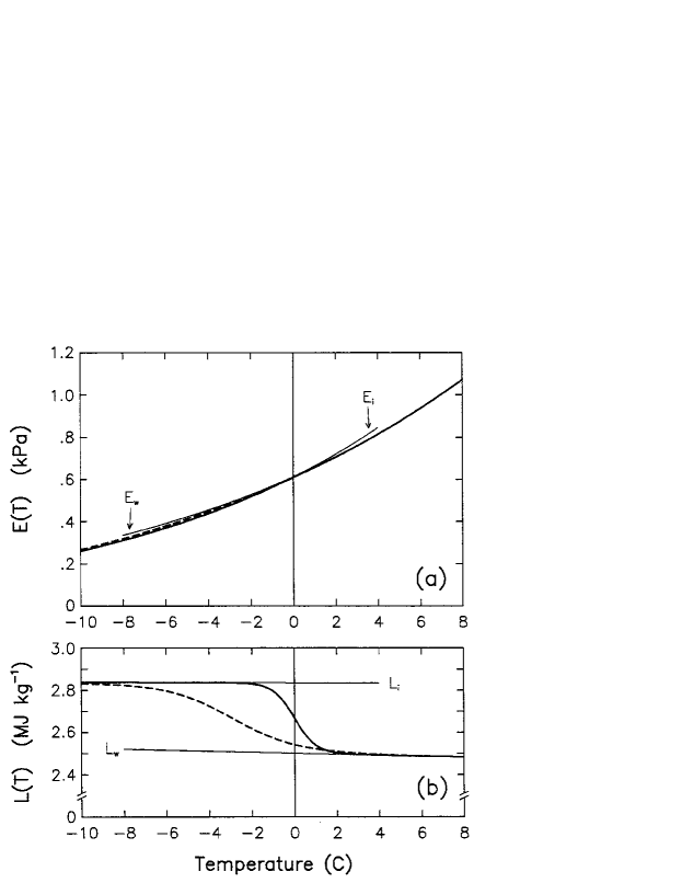
Figure 1: The top panel shows the saturation vapor pressure over ice, $E_{i}(T)$, and the saturation vapor pressure over water, $E_{w}(T)$, with $E_{w}>E_{i}$ for colder temperatures and $E_{i}>E_{w}$ for warmer temperatures. These empirical curves are based on laboratory results. They have been merged into a single synthetic profile with a sharp transition at $0^{\circ}$C (thick solid curve) and into a single synthetic profile with a gradual transition centered at $-3^{\circ}$C (dashed curve). The $E_{w}$ curve and the two synthetic curves are so close that they are indistinguishable on the right side of the upper panel. The lower panel shows the corresponding $L(T)$ curves, which are calculated from the Clausius-Clapeyron equation in the form $L(T)=R_{v}T^{2}[d\ln E(T)/dT]$. The difference between the asymptotic values $L_{i}$ and $L_{w}$ is the latent heat of fusion. Adapted from Ooyama (1990).

The thermodynamic diagnosis at each spatial point can be interpreted conceptually as the following input/output process:

$$\text{Input}\left\{\rho_{a},\rho_{m},\rho_{r},\sigma\right\}\Rightarrow\text{Output}\left\{\rho,T_{1},T_{2},\sigma_{r},T,\rho_{v},\rho_{c},p_{a},p_{v},p\right\}.$$

Specifically, starting with the values of the prognostic variables $\rho_{a},\rho_{m},\rho_{r},\sigma$, the thermodynamic diagnosis proceeds in the order given by (34)–(41), i.e., determination of the total density $\rho$ from (34), determination of the thermodynamically possible temperature $T_{2}$ from (35), the entropy density of precipitation from (36), the thermodynamically possible temperature $T_{1}$ from (37), the actual temperature $T$ of the gaseous matter from (38), the partial pressure of dry air from (39), the water vapor density $\rho_{v}$, cloud condensate density $\rho_{c}$, and water vapor partial pressure $p_{v}$ from the appropriate alternative in (40), and the total pressure $p$ from (41). Note that all the other required thermodynamic functions, such as $C(T)$, $D(T)$, $\rho_{v}^{*}(T)$, etc., can be determined from $E(T)$, once it is specified. If $E(T)$ is specified as $E_{w}(T)$ for all $T$, then the effects of the latent heat of fusion are not included. If a synthesized $E(T)$ is obtained from $E_{w}(T)$ and $E_{i}(T)$, then the effects of the latent heat of fusion are included.

To summarize, the procedure for advancing from one time level to the next consists of computing new values of the prognostic variables $\rho_{a},\rho_{m},\rho_{r},\sigma,u,v,w$ from (16)–(19) and the three momentum equations. The diagnostic variables required for the prognostic stage are determined by sequential evaluation of (34)–(41). Since they are not essential to our discussion here, we have omitted the parameterization formulas for the terminal fall velocity, $w_{\infty}$, and the source terms $Q_{r}$ and $Q_{\sigma}$.

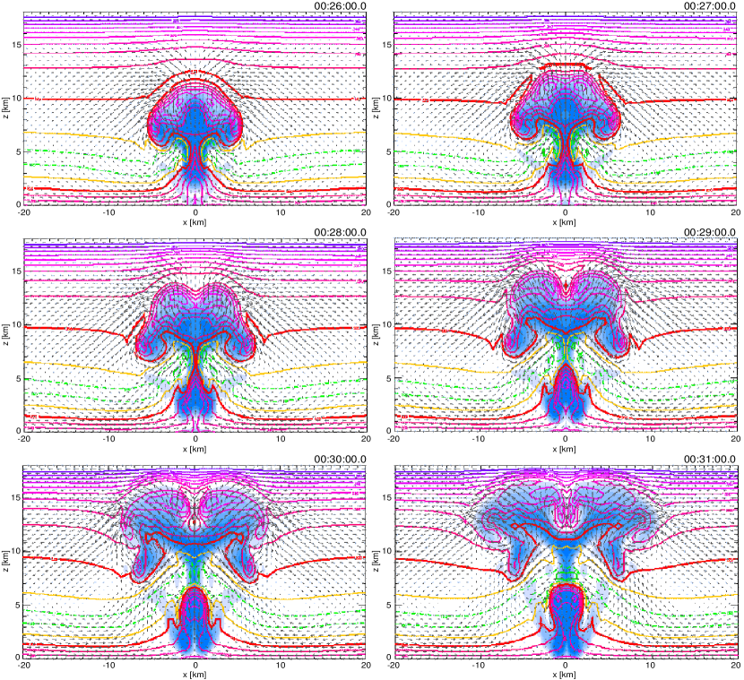
Figure 2: Development of a convective cell at one minute intervals using the nonhydrostatic moist model developed by Ooyama (1990, 2001). Model time is specified in the upper right of each panel, contour lines indicate the specific entropy of moist air, and blue shading indicates cloud boundaries and regions of precipitation. Note the transition from a plume of high $\theta_{e}$ air to a bubble structure below 5 km. Adapted from Garcia (1999).

It is interesting to note how the variation of $L$ with temperature is incorporated into this model. The idea is easily understood by reference to Fig. 1, the top panel of which shows the saturation vapor pressure over ice, $E_{i}(T)$, and the saturation vapor pressure over water, $E_{w}(T)$. Also shown are two merged $E(T)$ profiles, one with a sharp transition centered at $0^{\circ}$C (solid curve) and one with a gradual transition centered at $-3^{\circ}$C (dashed curve). The lower panel of Fig. 1 shows the two corresponding $L(T)$ curves, which have been calculated from the Clausius-Clapeyron equation in the form $L(T)=R_{v}T^{2}[d\ln E(T)/dT]$. The choice of the solid curve would produce model results with a sharp melting layer, while choice of the dashed curve would produce a melting layer several times as thick.

At present it is not feasible to numerically integrate such a nonhydrostatic “full physics" model over the whole globe with 1–2 km resolution. However, it is possible to perform such high resolution integrations over the limited area of a single tropical disturbance. Such integrations advance the art of tropical modeling to a new level that involves much less physical parameterization. An example of a high resolution simulation using this model is shown in Fig. 2, which depicts the development of convection in an environment at rest (Garcia 1999). For this simulation, the domain consists of 5 nested grids over a total horizontal distance of 1152 km. The finest (central) grid in this domain spans 96 km with a horizontal grid spacing of 0.5 km. The height of the domain is 18 km, with a constant vertical resolution of 750 m on all grids. The time integration for this simulation uses a semi-implicit formulation of the leapfrog method with a time step of 2.5 seconds on the finest grid. The initial background for this simulation consists of a mean hurricane season sounding which has been modified slightly to include higher relative humidity in the lower levels (surface to approximately 700 hPa) in order to better represent disturbed tropical conditions. The initial perturbation employed here was a thermal anomaly of $T^{\prime}=+3$K, centered at $x=0$, $z=0$ and with an overall width of 32 km. This figure depicts the development of the resulting convective cell at 1 minute intervals between 26 and 31 minutes of a 1 hour simulation. The line contours in Fig. 2 represent the dry-air-specific entropy of moist air as calculated by ${\mathcal{S}}=\sigma/\rho_{a}$. The contour interval is 10 J kg^-1 K^-1. The dry-air-specific entropy of moist air can also be interpreted in terms of equivalent potential temperature $\theta_{e}$ through the definition

$$\theta_{e}=T_{0}e^{{\mathcal{S}}/c_{pa}}\quad\Longleftrightarrow\quad{\mathcal{S}}=c_{pa}\ln(\theta_{e}/T_{0}).$$

Thus, ${\mathcal{S}}=$ 200 J kg^-1 K^-1 (the two neighboring green contours near $z\approx 4$ km in the cloud environment) correspond to $\theta_{e}=333$K, while the ${\mathcal{S}}=$ 250 J kg^-1 K^-1 contour near the surface in most of these panels corresponds approximately to $\theta_{e}=348$K. The blue shaded regions indicate the cloud water and precipitation content of the air: the lightest blue corresponds to cloud water in any concentration, while the darker blue shades represent precipitation content at intervals of $0.5$ g kg^-1. An interesting feature of Fig. 2 is the way in which the high $\theta_{e}$ contours (or, equivalently, the high $h$ contours) near the surface are drawn up in the convective plume during the first two minutes. These contours then close off and a bubble of high $\theta_{e}$ air is carried upward. Another interesting feature is the cap instability that develops near $z\approx 13$ km, above the rising convective plume. The $\bar{\rho}_{a}\overline{w^{\prime}{\mathcal{S}}^{\prime}}$ flux in (31) can be considered to be the result of a field of such convective clouds in various stages of their life cycles.

Numerous simulations have been performed with this model. These include simulations of tropical squall line systems (Ooyama 2001), and simulations of tropical cyclone development (Hausman et al. 2006) using an axisymmetric version of the model. In this regard it is interesting to note that such model simulations can lead to a better understanding of CAPE (or the cloud work function, which is a more general concept) and its generation by large-scale processes. To see why further understanding of convective energetics is needed, consider the following question. How do we define CAPE? The theory just described gives us at least eight ways! We can define a reversible adiabat (RA) with all condensate carried along with the parcel, and a pseudoadiabat (PA) with all condensate removed. Each of these can be defined with ice (wi) or with no ice (ni). Thus, we have four temperature profiles and four virtual temperature profiles for RA.wi, PA.wi, RA.ni, PA.ni. This gives eight ways of computing CAPE. Of course, we can also define CAPE in a myriad of ways which lie somewhere between RA and PA.

5 Concluding remarks

The main focus of our discussion has been the development of new, more accurate methods for the diagnostic analysis of heat and moisture budgets. The physical model which serves as the basis for this discussion is the nonhydrostatic moist model, consisting of (16)–(19) and three momentum equations. In this model, pressure is not used as one of the prognostic variables, since it is not a conservative property and its use as a prognostic variable would lead to an approximate treatment of moist thermodynamics. Rather, the prognostic variable for the thermodynamic state is $\sigma$, the entropy of moist air per unit volume, with temperature and total pressure (the sum of the partial pressures of dry air and water vapor) determined diagnostically. There are several unique aspects of this model which are worth noting. (1) The model dynamics are exact in the sense that there is no hydrostatic approximation. (2) The connection between dynamics and thermodynamics is through the gradient of pressure, which includes the partial pressures of dry air and water vapor. (3) The first law of thermodynamics is expressed in terms of $\sigma$, the entropy density of moist air; all the usual approximations associated with moist thermodynamics are thereby avoided. (4) There is no cumulus parameterization; the frontier of empiricism is pushed back to the microphysical parameterization of the precipitation process through $w_{\infty}$ and $Q_{r}$. (5) The model is modular in the sense that ice can be included by specifying $E(T)$ to be synthesized from the saturation formulas over water and ice.

In spite of the above unique aspects, the model thermodynamics should not be regarded as “exact." For example, the effects of the latent heat of fusion are always recognized in the same temperature interval (see Fig. 1), whether freezing is occurring on ascent or melting is occurring on descent. Hence, highly supercooled water in intense thunderstorm updrafts cannot be simulated. In any event, the concepts presented here open up the possibility of coordinated modeling and observational budget studies based on the same moist thermodynamic principles. At present, this research path remains largely unexplored.

References

- (1) Ciesielski, P. E., W. H. Schubert, and R. H. Johnson, 1999: Large-scale heat and moisture budgets over the ASTEX region. J. Atmos. Sci., 56, 3241–3261.
- (2) Gallus, W. A., and R. H. Johnson, 1991: Heat and moisture budgets of an intense midlatitude squall line. J. Atmos. Sci., 48, 122–146.
- (3) Garcia, M., 1999: Simulated Tropical Convection. M.S. Thesis, Dept. of Atmos. Science, Colorado State University, 270 pp.
- (4) Hausman, S. A., K. V. Ooyama, and W. H. Schubert, 2006: Potential vorticity structure of simulated hurricanes. J. Atmos. Sci., 63, 87–108.
- (5) Johnson, R. H., 1980: Diagnosis of convective and mesoscale motions during Phase III of GATE. J. Atmos. Sci., 37, 733–753.
- (6) Johnson, R. H., 1984: Partitioning tropical heat and moisture budgets into cumulus and mesoscale components: Implications for cumulus parameterization. Mon. Wea. Rev., 112, 1590–1601.
- (7) Johnson, R. H., and P. E. Ciesielski, 2000: Rainfall and radiative heating rates from TOGA-COARE atmospheric budgets. J. Atmos. Sci., 57, 1497–1514.
- (8) Johnson R. H., P. E. Ciesielski, and K. A. Hart, 1996: Tropical inversions near the 0∘C level. J. Atmos. Sci., 53, 1838–1855.
- (9) Johnson, R. H., P. E. Ciesielski, and T. M. Rickenbach, 2016: A further look at and from TOGA COARE. Multiscale Convection-Coupled Systems in the Tropics: A Tribute to Dr. Michio Yanai, Chap. 1, Meteorological Monographs, 56, American Meteorological Society, 1.1–1.12.
- (10) Johnson, R. H., P. E. Ciesielski, J. H. Ruppert Jr., and M. Katsumata, 2015: Sounding-based thermodynamic budgets for DYNAMO. J. Atmos. Sci., bf 72, 598–622.
- (11) Johnson R. H., and G. S. Young, 1983: Heat and moisture budgets of tropical mesoscale anvil clouds. J. Atmos. Sci., 40, 2138–2147.
- (12) Katsumata, M., P. E. Ciesielski, and R. H. Johnson, 2011: Evaluation of budget analysis during MISMO. J. Appl. Meteor. Clim., 50, 241–254.
- (13) Mapes, B. E., P. E. Ciesielski, and R. H. Johnson, 2003: Sampling errors in rawinsonde-array budgets. J. Atmos. Sci., 60, 2697–2714.
- (14) McNab, A. L., and A. K. Betts, 1978: A mesoscale budget study of cumulus convection. Mon. Wea. Rev., 102, 1317–1331.
- (15) Morrison, H., 2012: On the numerical treatment of hydrometeor sedimentation in bulk and hybrid bulk-bin microphysics schemes. Mon. Wea. Rev., 140, 1572–1588.
- (16) Nitta, T., 1975: Observational determination of cloud mass flux distribution. J. Atmos. Sci., 32, 73–91.
- (17) Nitta, T., and S. Esbensen, 1974: Heat and moisture budget analyses using BOMEX data. Mon. Wea. Rev., 102, 17–28.
- (18) Ogura, Y., and H.-R. Cho, 1973: Diagnostic determination of cumulus populations from large-scale variables. J. Atmos. Sci., 30, 1276–1286.
- (19) Ooyama, K. V., 1990: A thermodynamic foundation for modeling the moist atmosphere. J. Atmos. Sci., 47, 2580–2593.
- (20) Ooyama, K. V., 2001: A dynamic and thermodynamic foundation for modeling the moist atmosphere with parameterized microphysics. J. Atmos. Sci., 58, 2073–2102.
- (21) Schumacher, C., M. H. Zhang, and P. E. Ciesielski, 2007: Heating structures of the TRMM field campaigns. J. Atmos. Sci., 64, 2593–2610.
- (22) Schumacher, C., P. E. Ciesielski, and M. H. Zhang, 2008: Tropical cloud heating profiles: Analysis from KWAJEX. Mon. Wea. Rev., 136, 4348–4364.
- (23) Xie, S., R. T. Cederwall, and M. Zhang, 2004: Developing long-term single-column model/cloud system-resolving model forcing data using numerical weather prediction products constrained by surface and top of the atmosphere observations. J. Geophys. Res., 109, D01104, 12pp.
- (24) Yanai, M., S. Esbensen, and J.-H. Chu, 1973: Determination of bulk properties of tropical cloud clusters from large-scale heat and moisture budgets. J. Atmos. Sci., 30, 611–627.
- (25) Yanai, M., and R. H. Johnson, 1993: Impacts of cumulus convection on thermodynamic fields. The Representation of Cumulus Convection in Numerical Models of the Atmosphere, Meteorological Monographs, 46, American Meteorological Society, 39–62.
- (26) Zhang, M. H., and J. L. Lin, 1997: Constrained variational analysis of sounding data based on column-integrated budgets of mass, heat, moisture, and momentum: Approach and application to ARM measurements. J. Atmos. Sci., 54, 1503–1524.
- (27) Zhang, M. H., J. L. Lin, R. T. Cederwall, J. J. Yio, and S. C. Xie, 2001: Objective analysis of ARM IOP Data: Method and sensitivity. Mon. Wea. Rev., 129, 295–311.
- (28)