Gravitational waves from global cosmic strings in quintessential inflation

Abstract

The combination of non-minimal couplings to gravity with the post-inflationary kinetic-dominated era typically appearing in quintessential inflation scenarios may lead to the spontaneous symmetry breaking of internal symmetries and its eventual restoration at the onset of radiation domination. On general grounds, the breaking of these symmetries leads to the generation of short-lived topological defects that tend to produce gravitational waves until the symmetry is restored. We study here the background of gravitational waves generated by a global cosmic string network following the dynamical symmetry breaking and restoration of a $U(1)$ symmetry. The resulting power spectrum depends on the duration of the heating process and it is potentially detectable, providing a test on the existence of non-minimal couplings to gravity and the characteristic energy scale of post-inflationary physics.

1 Introduction

The direct detection of gravitational waves (GW) from black hole and neutron star mergers [1, 2, 3], together with the observation of an electromagnetic counterpart [4], have opened a new window for observational cosmology. Interestingly, these individual two-body sources are just one of the many signals that could be detected by present and future experiments. A stochastic background of GWs could be produced, for instance, during inflation and (re)heating [5, 6, 7] or be associated with exotic post-inflationary physics such as phase transitions or topological defects [8, 9, 10, 11, 12, 13]. The discovery of any of these backgrounds would provide an extremely valuable piece of information on energy scales much beyond the reach of any particle physics accelerator.

Topological defects are created whenever there is a spontaneous symmetry breaking, usually associated with some critical temperature. A temporary network of these objects is also expected in the presence of non-minimal couplings to gravity, provided the existence of a kinetic dominated era with stiff equation-of-state parameter $w>1/3$ [14]. In this paper, we argue that a stochastic background of GWs could be produced by a temporary network of cosmic string appearing in quintessential inflationary models with non-oscillatory runaway potentials. The main ingredient of our proposal is a subdominant non-minimally coupled $U(1)$ scalar field on top of the inflaton and matter sectors. The non-minimal coupling to gravity renders heavy the $U(1)$ field during inflation, preventing the generation of dangerous isocurvature perturbations [14].

After inflation, where the violation of the slow-roll conditions together with the absence of a minimum for the inflaton field leads to the onset of a kinetic-dominated era, the Ricci scalar turns negative and with it the effective mass of the $U(1)$ field. The symmetry becomes then spontaneously broken and the field develops a new vacuum at large field values, leading to the formation of a cosmic string network by the standard Kibble mechanism [11]. The oscillations of the strings within the Hubble volume generate a GWs spectrum with an energy density that becomes cumulatively enhanced with respect to the rapidly decreasing energy density of the kinetic-dominated background. The production of GWs continues till the onset of the hot big bang era, where the Ricci scalar vanishes and the negative mass term enforcing the symmetry breaking effectively disappears. When that happens, the initial symmetry is restored and the origin becomes again the absolute minimum of the potential. The complex $U(1)$ field starts spiraling around it, destroying the cosmic string network and halting the GW production. Since the spectrum of GWs is frozen during the long-lasting radiation-dominated era, the final energy density in GWs remains essentially unchanged up to the present cosmological epoch.

This paper is organized as follows. In Section 2 we recapitulate the most important aspects of quintessential inflation. The dynamics of a subdominant non-minimally coupled $U(1)$ field in this cosmological background is described in Section 3. Section 4 discuss the formation of cosmic strings and the salient features of the associated GW spectrum. Section 5 is devoted to the computation of the present day GW spectrum and to the discussion of the constraints that present and future experiments could cast on the model parameters and early universe physics. Finally, our conclusions are drawn in Section 6.

2 Quintessential inflation

Inflation and dark energy are usually understood as two independent epochs in the history of the Universe. Note, however, that there is no fundamental reason for this to be the case. The common features of these cosmological periods could be related, for instance, to some underlying principle, such as the explicit [15, 16, 17] or emergent realization of scale invariance in the vicinity of non-trivial fixed points [18, 19, 20, 21]. A framework that fits well with the last possibility is quintessential inflation [22, 23, 24, 25, 26, 27, 28, 21]. In its simplest terms, this paradigm makes use of a single degree of freedom — dubbed cosmon [29] — to provide a unified description of inflation and dark energy. Although certain parametrizations involving a non-canonical cosmon field are certainly preferred to highlight the aforementioned connection to scale symmetry [18, 19, 20, 21], we will follow here the standard approach and describe quintessential inflation in terms of a canonically normalized cosmon field $\phi$ with Lagrangian density

$$\frac{\cal L}{\sqrt{-g}}=\frac{M_{\rm P}^{2}}{2}R-\frac{1}{2}\partial_{\mu}\phi\partial^{\mu}\phi-U(\phi)\,,$$ (2.1)

where $M_{\rm P}=(8\pi G)^{-1/2}$ is the reduced Planck mass and $R$ is the Ricci scalar. A particular model within the paradigm is specified by a choice of the potential $U(\phi)$, which is required to be of the runaway form in order to support inflation and dark energy. Several quintessential potentials have been proposed in the literature [18, 19, 30, 20, 25, 21, 31], each of them leading to slightly different predictions for the inflationary and dark energy observables. Despite numerical dissimilarities, the background evolution of the Universe is rather insensitive to the precise form of $U(\phi)$ and involves always the same sequence of cosmological epochs. At early times, the scalar field is generically displaced at large field values, allowing for inflation with the standard chaotic initial conditions. The inflationary epoch will end, as usual, when the kinetic energy density of the cosmon starts to dominate over the potential counterpart, signaling the break-down of the slow-roll approximation. In the absence of a potential minimum, the Universe will inevitably enter a kination or deflation era with effective equation-of-state parameter $w=1$ [23]. The duration of this unusual cosmological epoch depends on the efficiency of the heating process.

A plethora of heating mechanisms within quintessential inflation have been proposed in the literature [32, 33, 22, 34, 35, 36, 21, 37, 38]. All these mechanisms share a common feature: the decay of the inflaton field does not need to be complete. Even if the initial particle creation is small, the rapid decrease of the cosmon energy density during kinetic domination ($\rho_{\phi}\sim a^{-6}$) as compared to the redshift of the created plasma $(\rho_{\rm R}\sim a^{-4})$ will eventually lead to radiation domination. A useful way of parametrizing the duration of this transition period is to make use of a heating efficiency parameter [21]

$$\Theta\equiv\frac{\rho_{\rm R}^{\rm kin}}{\rho^{\rm kin}_{\phi}}=\left(\frac{a_{\rm kin}}{a_{\rm rad}}\right)^{2}\,,$$ (2.2)

where $\rho^{\rm kin}_{\phi}$ and $\rho_{\rm R}^{\rm kin}$ stand for the energy density of the cosmon and the heating products at the beginning of kinetic domination and $a_{\rm kin}$ and $a_{\rm rad}$ denote respectively the values of the scale factor at the onset of kinetic and radiation domination. For a fiducial Hubble rate $H_{\rm kin}\sim 10^{11}\,{\rm GeV}$, the typical heating efficiencies per degree of freedom vary between $\Theta\sim 10^{-19}$ in gravitational heating scenarios [32, 33, 22] and $\Theta\sim{\cal O}(1)$ in heating scenarios involving matter fields [34, 21]. The minimal value of $\Theta$ is restricted by big bang nucleosynthesis, where the standard hot big bang history should be definitely recovered. In particular, quintessential inflation generates a primordial gravitational wave background that becomes blue tilted during kinetic domination [39, 21],

$$\Omega_{\rm GW}(k)\sim k\,,$$ (2.3)

and may excessively contribute to the effective number of relativistic degrees of freedom at big bang nucleosynthesis, modifying with it the light elements’ abundance. The (integrated) nucleosynthesis constraint on the GW density fraction [40, 41],

$$h^{2}\int_{k_{\rm BBN}}^{k_{\rm end}}\Omega_{\rm GW}(k)\,d\ln k\lesssim 1.12\times 10^{-6}\,,$$ (2.4)

with $h=0.678$ and $k_{\rm end}$ and $k_{\rm BBN}$ the momenta associated to the horizon scale at the end of inflation and at big bang nucleosynthesis, translates into a lower bound on the heating efficiency [21]

$$\Theta\gtrsim 10^{-16}\left(\frac{H_{\rm kin}}{10^{11}\,{\rm GeV}}\right)^{2}\,,$$ (2.5)

which should be compared with the efficiency of a given heating scenario.

Beyond the onset of radiation domination, the background follows the usual hot big bang evolution  [21]. At the early stages of radiation domination, the cosmon field freezes to a constant value, allowing for the resurgence of its potential energy density. When this component re-approaches the decreasing energy density of the radiation fluid, the evolution of the system settles down to a scaling solution in which the scalar energy density tracks the background evolution [42, 43]. Eventually the cosmon will exit the tracking regime, leading to a dark energy dominated era  [42, 44].

3 Non-minimally coupled spectator field dynamics

Let us study the dynamics of a subdominant non-minimally coupled $U(1)$ scalar field in the quintessential inflation scenario discussed in the previous section. To this end, we consider a Lagrangian density

$$\frac{\mathcal{L}_{\chi}}{\sqrt{-g}}=-\partial_{\mu}\chi^{\dagger}\partial^{\mu}\chi-\left(m_{\chi}^{2}+\xi R\right)\chi^{\dagger}\chi-\lambda\frac{(\chi^{\dagger}\chi)^{\frac{n}{2}}}{\Lambda^{n-4}}\,,$$ (3.1)

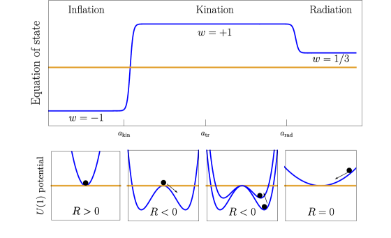
Figure 1: Schematic behaviour of the $U(1)$ potential and of the $\chi$ field evolution during the different cosmological epochs in quintessential inflationary scenarios. The horizontal lines correspond to the zero value of the corresponding quantity.

with $m_{\chi}^{2}$ a bare mass parameter, $\xi$ is a positive dimensionless parameter, $\lambda$ a positive dimensionless coupling, $n\geq 4$ and $\Lambda$ a cutoff scale (a priori unknown). The non-minimal coupling to gravity is motivated by quantum field computations in curved spacetime [45] and its associated phenomenology has been widely studied in the literature, with applications in baryogenesis [14], (re)heating [37] and dark matter production [46, 47].

Rather than specifying a particular quintessential inflation potential in Eq. (2.1), we will follow here a model-independent approach and describe the background evolution of the Universe in terms of the Ricci scalar behaviour at the different cosmological epochs. For a flat Friedmann-Lemaitre-Robertson-Walker background metric $g_{\mu\nu}={\rm diag}(-1,a^{2}(t)\,\delta_{ij})$, the Ricci scalar in Eq. (3.1) can be written as

$$R=3(1-3w)H^{2}\,,$$ (3.2)

with $H=\dot{a}/a$ the Hubble rate and $w$ the equation-of-state of the dominant energy component.

The evolution of the $U(1)$ potential is summarized in Fig. 1. During the inflationary stage, the parameter $w$ approaches the de Sitter value $w\simeq-1$ and the Ricci scalar is constant and positive,

$$R=12H^{2}\,.$$ (3.3)

The mass term for the $\chi$ field in Eq. (3.1) is then also positive definite and the ground state of the system is located at the origin of the effective potential, $|\chi_{\rm min}|=0$. This implies, not only the $U(1)$ symmetry is preserved, but also that the $U(1)$ field is heavy during inflation and no sizable isocurvature perturbations are generated [14].

As soon as the slow-roll conditions are violated, the system enters a deflation period with stiff equation-of-state parameter $w=1$. During this era, the Ricci scalar flips sign

$$R=-6H^{2}\,.$$ (3.4)

If the associated Hubble-induced mass in Eq. (3.1) exceeds the bare mass of the $\chi$ field at that time, the $U(1)$ symmetry becomes spontaneously broken. When that happens, the field starts rolling down from the origin to the new minimum of the potential, which is time-dependent and located at

$$|\chi_{\rm min}(a)|=|\chi_{\rm min}(a_{\rm kin})|\left(\frac{a}{a_{\rm kin}}\right)^{-\frac{6}{n-2}}\,,\hskip 28.45274pt|\chi_{\rm min}(a_{\rm kin})|\simeq\left[\frac{12\,\xi}{n\lambda}\left(\frac{H_{\rm kin}}{M_{P}}\right)^{2}\left(\frac{\Lambda}{M_{P}}\right)^{n-4}\right]^{\frac{1}{n-2}}M_{P}\,.$$ (3.5)

During the first stages of kinetic domination, the higher dimensional operators in Eq. (3.1) can be safely neglected. In this case, the evolution of the field in its way to the time-dependent minimum (3.5) can be well-described by the approximate solution [37, 14]

$$|\chi(a)|\simeq|\chi(a_{\rm kin})|\left(\frac{a}{a_{\rm kin}}\right)^{\sqrt{6\xi}}\,,\hskip 42.67912pt|\chi(a_{\rm kin})|\equiv\frac{1+\sqrt{6\xi}}{2\sqrt{2}\pi}H_{\rm kin}\,,$$ (3.6)

where we have neglected the subleading mass term $m_{\chi}$ and assumed standard vacuum fluctuations as initial conditions. An estimate of the number of e-folds $\Delta N_{\rm tr}$ needed to reach (3.5) can be obtained by equating $|\chi(a_{\rm tr})|=|\chi_{\rm min}(a_{\rm tr})|$ with $a_{\rm tr}$ the value of the scale factor at the transition time,

$$\Delta N_{\rm tr}\equiv\ln\left(\frac{a_{\rm tr}}{a_{\rm kin}}\right)=\frac{n-2}{(n-2)\sqrt{6\xi}+6}\ln\left[\frac{|\chi_{\rm min}(a_{\rm kin})|}{|\chi(a_{\rm kin})|}\right]\,,$$ (3.7)

Once in the minimum, the field tracks its evolution until the $U(1)$ symmetry is restored. Then, the origin becomes again the ground state of the system and the spectator field $\chi$ starts oscillating around it, provided that the bare mass $m_{\chi}$ exceeds the instantaneous Hubble rate at the time. If this is not the case, the field will stay frozen at its restoration value until the Hubble parameter has decreased enough to allow for the oscillations.

4 Cosmic string network and GW production

At the onset of kinetic domination the phases of the $U(1)$ field are randomly distributed, with a correlation length of the order of the Hubble parameter at that time [48]. As soon as the horizon expands, multiple patches with different phases enter in causal contact, leading to the formation of a cosmic string network [49]. The spontaneous breaking of the global $U(1)$ symmetry comes associated with a massless Goldstone boson, which mediates a long-range interaction among the strings and keeps their energy density finite by effectively introducing a radial cut-off.  The width of the cosmic strings is inversely proportional to the expectation value of the $\chi$ field, which, as shown in Eq (3.6), rapidly increases during the first stages of kinetic domination. Since the Hubble rate is the only relevant scale in our model, we have “fat” strings with a width $\sim H^{-1}$ soon after the spontaneous symmetry breaking.

Fat strings like the ones under consideration have been extensively studied in the context of axion dark matter [51, 52, 53], finding an average of one string per Hubble volume. In our case, this is even more expected since the width of the string is already proportional to the Hubble rate at the time of formation. Note that this unusual property restricts the formation of cosmic string loops, since the length of these objects cannot be — for obvious reasons — shorter than its width. This allows us to neglect the (usually dominant) GW production by loops [54, 55, 56] and estimate the total energy density of the network by computing the energy density stored in a single string of Hubble length $L\propto H^{-1}$ within a Hubble volume $H^{3}$, namely

$$\rho_{\rm cs}\approx\mu(t)\times L\times H^{3}\approx\mu(t)H^{2}\,,$$ (4.1)

with

$$\mu(t)\sim|{\chi}(t)|^{2}\,,$$ (4.2)

the energy of the string per unit length. Note that the relative energy density of the strings as compared to the background component depends on time,

$$\Omega_{\rm cs}\equiv\frac{\rho_{\rm cs}}{3H^{2}M_{\rm P}^{2}}\sim\frac{\mu(t)}{M_{\rm P}^{2}}\sim\frac{|\chi(t)|^{2}}{M^{2}_{\rm P}}\,,$$ (4.3)

meaning that an exact scaling regime [57, 58, 59, 60] is never achieved. This is not necessarily a problem as long as the energy density of cosmic strings stays subdominant with respect to the background component, i.e. $\Omega_{\rm cs}\ll 1$. This consistency condition translates into a limit on the maximum value that can be explored by the $U(1)$ field, restricting it be sub-Planckian,

$$|\chi(t_{\rm tr})|\ll M_{P}\,.$$ (4.4)

and setting a maximum on the number of e-folds (3.7) required to arrive to the time-dependent minimum (3.5),

$$\Delta N_{\rm tr}\ll\frac{1}{\sqrt{6\xi}}\left[18+\ln\left(\frac{1}{1+\sqrt{6\xi}}\right)+\ln\left(\frac{10^{11}\,{\rm GeV}}{H_{\rm kin}}\right)\right]\,.$$ (4.5)

In the presence of a scaling regime, the evolution of the cosmic strings’ energy momentum tensor in the vicinity of the horizon leads to the production of a scale-invariant gravitational wave spectrum [61] (for a recent review see Ref. [41]). Note, however, that the vacuum expectation value of the scalar field in our scenario evolves with time. We expect therefore a residual scale dependence in the spectrum, measured exactly by the change of this quantity. The amount of GWs produced by a vibrating string of length $L\propto H^{-1}$ can be estimated by approximating the associated quadrupole $Q$ by that of a cylinder of mass $M\approx\mu\,L$ and width $R\propto H^{-1}$ [61, 40], namely

$$Q(t)\propto MR^{2}\sim\mu(t)H^{-3}\,,$$ (4.6)

with the precise proportionality constant depending on the level of non-sphericity of the configuration. Assuming that the relaxation time is of the order of $H$, the luminosity in GWs becomes

$$\mathcal{L}(t)\sim M_{\rm P}^{-2}\,\dddot{Q}(t)^{2}\sim M_{\rm P}^{-2}(H^{3}(t)Q(t))^{2}\sim\mu^{2}(t)M_{\rm P}^{-2}\,,$$ (4.7)

where we have replaced time derivatives in favor of the Hubble parameter $H$. At a given instant $t$, the emission of GWs is peaked around the characteristic scale of the system at that time, decaying as a power-law for shorter and longer distances. The relative power emitted by the string network in a Hubble time (i.e. per $dN\equiv Hdt$) is given by [62]

$$\frac{\Delta P_{\rm GW}(t,k)}{\Delta N}\equiv\frac{1}{3H^{2}M_{\rm P}^{2}}\frac{d\rho_{\rm GW}(t,k)}{d\log k}\simeq\begin{cases}P_{\rm peak}(t)\left(\frac{k}{k_{\rm peak}(t)}\right)^{\alpha}\hskip 19.91692pt{\rm for}\hskip 14.22636ptk\lesssim k_{\rm peak}\,,\\ P_{\rm peak}(t)\left(\frac{k}{k_{\rm peak}(t)}\right)^{-\bar{\alpha}}\hskip 14.22636pt{\rm for}\hskip 14.22636ptk>k_{\rm peak}\,,\\ \end{cases}$$ (4.8)

with $k_{\rm peak}(t)\sim aH$ the peak emission wavenumber and

$$P_{\rm peak}(t) \sim \frac{L^{-2}\times\mathcal{L}}{H^{2}M_{\rm P}^{2}}\sim\frac{\mathcal{L}}{M_{\rm P}^{2}}\sim\left(\frac{|\chi(t)|}{M_{\rm P}}\right)^{4}\,.$$ (4.9)

The exponents $\alpha$ and $\bar{\alpha}$ in Eq. (4.8) parametrize our ignorance about the exact momentum dependence. While a scaling $\alpha=2$ can be inferred from simple causality arguments  [63, 62], the value of $\bar{\alpha}$ must be derived from simulations. Note, however, that this exponent is intimately related to the dynamics of small scales and it should be therefore rather independent of the specific expansion history. This observation allows us to benefit from existing numerical results to set a fiducial value $\bar{\alpha}\sim 2$  [62].

4.1 GW spectrum in a generic background

The precise form of the accumulated GW spectrum at large momenta is obtained by integrating Eq. (4.8) from the time $t_{\rm i}$ at which the strings start to form to an arbitrary time $t$ that will be later associated with the moment at which strings decay and the production of GWs is halted. Since the emission peak in our scenario is set by the comoving horizon, $k_{\rm peak}\sim aH=\tau^{-1}$, it is convenient to work in conformal time $\tau$. In terms of this time coordinate, the integrated GW spectrum takes the form

$$\Omega_{\rm GW}\left(\tau,k\right)=\int^{\tau}_{\tau_{\rm i}}d\log\tau^{\prime}\frac{\Delta P_{\rm GW}(\tau^{\prime},k)}{\Delta\log\tau^{\prime}}\left(\frac{a(\tau^{\prime})}{a(\tau)}\right)^{b}\,,$$ (4.10)

where we have used the fact that $dN\propto d\log\tau$ and accounted for the evolution of the GW energy density. For the sake of completeness and in order to facilitate the comparison with other works in the literature, we have considered a generic power-law evolution $a\sim t^{p}\sim\tau^{p/(1-p)}$ with $p$ a constant.  The scaling power $b$ in Eq. (4.10) is related to $p$ via $b\equiv 4-2/p$ and takes values $b=-2$ and $b=0$ during kination and radiation domination.

We can distinguish two possible scenarios depending on the relation between the bare mass $m_{\chi}$ and the Hubble rate $H_{\rm rad}$ at the time of heating:

1. If $m_{\chi}\geq H_{\rm rad}$ the symmetry is restored before radiation domination and the $U(1)$ scalar field is free to oscillate around the origin, leading to the evanescence of the cosmic string network and halting the GW production.

2. If $m_{\chi}<H_{\rm rad}$ the $U(1)$ field remains frozen at its vacuum expectation value after symmetry restoration. Although additional strings are no longer generated, the existing ones will continue producing GWs after reentering the expanding horizon. This GW production will stop when the instantaneous Hubble rate becomes comparable to the mass of the field, $H\lesssim m_{\chi}$. From there on, the field $\chi$ will start oscillating around the origin and the strings will consequently decay.

Since the use of numerical simulations is most probably required in the latest scenario, we will focus here on the $m_{\chi}\geq H_{\rm rad}$ case. The total power in GWs produced by the cosmic string network can be then computed by integrating Eq. (4.10) from the formation time $\tau_{i}$ to the time $\tau=\tau_{\rm osc}$ at which the symmetry is restored. Taking into account Eq. (4.8) we can rewrite this expression as [62]

$$\Omega_{\rm GW}\left(\tau_{\rm osc},k\right) \simeq \int^{\tau_{k}}_{\tau_{\rm i}}\frac{d\tau^{\prime}}{\tau^{\prime}}P_{\rm peak}(\tau^{\prime})\left(\frac{k}{k_{\rm peak}(\tau^{\prime})}\right)^{\alpha}\left(\frac{a(\tau^{\prime})}{a(\tau)}\right)^{b}$$ (4.11)

$$+ \int^{\tau_{\rm osc}}_{\tau_{k}}\frac{d\tau^{\prime}}{\tau^{\prime}}P_{\rm peak}(\tau^{\prime})\left(\frac{k}{k_{\rm peak}(\tau^{\prime})}\right)^{-\bar{\alpha}}\left(\frac{a(\tau^{\prime})}{a(\tau)}\right)^{b}\,,$$

where we have defined $\tau_{k}$ as the time at which the peak emission mode coincides with the mode $k$, i.e. $k_{\rm peak}(\tau_{k})=k$. This splitting takes into account the amount of time that each mode spends in the blue or red part of the spectrum given that the peak is evolving with time. Also notice that, since we require that $\tau_{k}>\tau$, the integral is only valid for $k>k_{\rm peak}(\tau)$ [62].

The integrated GW spectrum in Eq. (4.11) has three main contributions. On the one hand, we have two associated with the blue-shifting of the power spectrum itself, which give either a $k^{-\bar{\alpha}}$ or a $k^{\alpha}$ scaling depending on how much time did the wavenumber $k$ spend in each slope. On the other hand, we have the contribution coming from the time at which the mode $k$ coincides with the generic time-dependent peak emission mode $k_{\rm peak}(\tau_{k})$. In that case the power spectrum is evaluated at $k\,\tau_{k}\sim 1$. Assuming a generic power-law dependence $P_{\rm peak}\sim\tau^{-\gamma}$ with constant parameter $\gamma$,  this leads to a scaling $\Omega_{\rm GW}\sim k^{\beta}$ with

$$\beta\equiv\gamma-\frac{4\,p-2}{1-p}\,.$$ (4.12)

The above contributions compete in the integrated form of Eq. (4.11) yielding 

$$\Omega_{\rm GW}\left(\tau_{\rm osc},k\right) \simeq P_{\rm peak}(\tau_{\rm osc})\left(\frac{k}{k_{\rm peak}(\tau_{\rm osc})}\right)^{\beta}\times$$ (4.13)

$$\times \left[\frac{1}{\beta-\alpha}\left(\left(\frac{k_{\rm peak}(\tau_{\rm i})}{k}\right)^{\beta-\alpha}-1\right)\frac{1}{\bar{\alpha}+\beta}\left(1-\left(\frac{k_{\rm peak}(\tau_{\rm osc})}{k}\right)^{\bar{\alpha}+\beta}\right)\right]\,.$$

This analytical expression explores a range of frequencies comprised between $k_{\rm peak}(\tau_{\rm osc})\leq k\leq k_{\rm peak}(\tau_{\rm i})$. For intermediate frequencies well within the integration limits, $k_{\rm peak}(\tau_{\rm osc})\ll k\ll k_{\rm peak}(\tau_{\rm i})$, we can identify three regimes depending on the sign of $\beta-\alpha$ and $\beta+\bar{\alpha}$, namely

$$\Omega_{\rm GW}\propto\begin{cases}k^{\alpha}\hskip 19.91692pt{\rm for}\hskip 14.22636pt\beta-\alpha>0\,,\\ k^{\beta}\hskip 19.91692pt{\rm for}\hskip 14.22636pt\beta-\alpha<0\quad\text{and}\quad\bar{\alpha}+\beta>0\,,\\ k^{-\bar{\alpha}}\hskip 14.22636pt{\rm for}\hskip 14.22636pt\beta-\alpha<0\quad\text{and}\quad\bar{\alpha}+\beta<0\,.\\ \end{cases}$$ (4.14)

Since $\alpha>0$, the first case corresponds to a blue-tilted spectrum while the second one can be either blue or red depending on the sign of $\beta$, which is ultimately determined by the evolution of the $\chi$ field and the background, cf. Eq. (4.12). Finally, the last case corresponds to a red tilted spectrum since $\bar{\alpha}>0$ [62].

4.2 GW spectrum in quintessential inflation

The formalism presented in the previous section is quite general and holds for any background and temporal dependence of the emission peak, as long as this can be parametrized by a power law $P_{\rm peak}\sim\tau^{-\gamma}$ with $\gamma$ approximately constant for some temporal interval $\Delta\log\tau$. In this section, we particularize our results to the kinetic-dominated era appearing in our quintessential inflation scenario, determining the precise form of $\gamma$ and the power spectrum as a function of the model parameters.

The background evolution during kinetic domination is specified by taking $p=1/3$ and hence $b=-2$. During this epoch, the dynamics of the scalar field $\chi$ can be split into a rolling and a minimum phase, each of them leading to different characteristic shapes in the GWs spectrum. The first phase is associated with the initial stages of kination, where the $U(1)$ scalar field is still rolling down the origin towards the Hubble-induced minimum of the potential. The second phase describes the tracking of the minimum once the field reaches it, if it does. We refer the interested reader to the Appendix A, where a detailed calculation of the GW spectrum is performed. Here we will simply discuss the shape of the spectrum and its dependence on the parameters.

Phase	$\alpha$	$\hskip 5.69054pt\bar{\alpha}$	$\beta$	$\hskip 14.22636pt\gamma$	$\beta-\alpha$	$\bar{\alpha}+\beta$	tilt range
Rolling	2	$\hskip 5.69054pt\sim 2$	$1-2\sqrt{6\xi}$	$\hskip 5.69054pt-2\sqrt{6\xi}$	$-1-2\sqrt{6\xi}$	$3-2\sqrt{6\xi}$	$1$ to $-2$
Minimum	2	$\hskip 5.69054pt\sim 2$	$\dfrac{10+n}{n-2}$	$\dfrac{12}{n-2}$	$\dfrac{14-n}{n-2}$	$3\dfrac{n+2}{n-2}$	$1$ to $2$

Table 1: Values of the spectrum powers during the rolling and the minimum phase. The value of $\gamma$ has been extracted from Eqs. (3.5), (3.6) into (4.9). The tilt range has been computed using Eq. (4.14) taking the formal limits $\xi\rightarrow 0$, $\xi\rightarrow\infty$ and $n\rightarrow 4$, $n\rightarrow\infty$, respectively.

In particular, we report in Table 1 the values of the power law indexes during the various stages. Note that the parameter $\gamma$ is negative during the rolling phase $(\tau<\tau_{\rm tr})$ and positive definite during the minimum phase $(\tau>\tau_{\rm tr})$. As shown in the last column, the spectrum of GWs during the rolling phase can be both blue and red depending on the values of the parameter $\xi$, namely

$$\Omega_{\rm GW}(\tau,k>k_{\rm tr})\propto\begin{cases}k^{1+\gamma}\hskip 14.22636pt{\rm if}\hskip 14.22636pt\xi<3/8\,,\\ k^{-\bar{\alpha}}\hskip 19.91692pt{\rm if}\hskip 14.22636pt\xi>3/8\,.\end{cases}$$ (4.15)

On the other hand, the spectrum during the minimum phase can only be blue, with the precise tilt depending on the order of the higher-order operators in Eq. (3.1),

$$\Omega_{\rm GW}(\tau,k<k_{\rm tr})\propto\begin{cases}k^{1+\gamma}\hskip 19.91692pt{\rm if}\hskip 14.22636ptn>14\,,\\ k^{\alpha}\hskip 28.45274pt{\rm if}\hskip 14.22636ptn<14\,.\end{cases}$$ (4.16)

The integrated GW spectrum when both phases are present can be generically written as an amplitude times a $k$-dependent form function, namely

$$\Omega_{\rm GW}(\tau_{\rm osc},k)\sim P_{\rm peak}(\tau_{\rm kin})\Theta^{-1}\left(\frac{a_{\rm osc}}{a_{\rm rad}}\right)^{2}F\left(\kappa,s_{\rm osc},s_{\rm tr}\right)\,,$$ (4.17)

where the blue-shifting factor $a_{\rm osc}/a_{\rm rad}$ appears because we factored out $\Theta^{-1}$ and we have defined the dimensionless variables

$$s\equiv\frac{\tau}{\tau_{\rm kin}}\hskip 34.1433pt\text{and}\hskip 34.1433pt\kappa\equiv\frac{k}{a_{\rm kin}H_{\rm kin}}\,.$$ (4.18)

The functional $F$ encodes the momentum behavior of the spectrum as a function of the model parameters. A detailed computation of this quantity assuming a sudden transition between the rolling and the minimum phases can be found in the Appendix A.

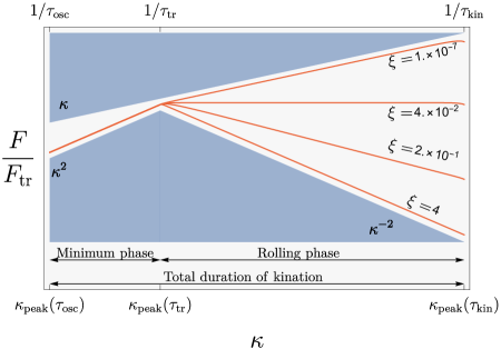
Figure 2: Form of the function $F$ in Eq. (4.17) for various values of $\xi$. The shaded area represents the asymptotic values reported in Table 1. Here we have assumed $a_{\rm osc}=a_{\rm rad}$ and $n=4$.

As illustrated in Figure 2, the shape of the spectrum is determined by the values of the $\alpha$, $\bar{\alpha}$ and $\beta$ parameters, according to the discussion in Eq. (4.14). In particular, the two stages of evolution give rise to two spectral indexes, hence to an inflection point in the spectrum. We can distinguish three characteristic $k$ values, namely $k_{j}\equiv a(\tau_{j})H(\tau_{j})$ with $j={\rm kin},{\rm tr},{\rm rad}$ standing respectively for the symmetry breaking time, the onset of the minimum phase and that of radiation domination. For each of these modes the amplitude of the power spectrum can be determined as follows: using Eq. (A.7) one can get the amplitude for $k=k_{\rm kin}$ and then use the scaling in Eqs. (4.15) and (4.16) to compute the amplitude for the other two modes. Assuming for simplicity that both phases are present and that they have a duration of several e-folds, i.e. $k_{\rm rad}\ll k_{\rm tr}\ll k_{\rm kin}$, i.e. we get

$$\Omega_{\rm GW}(\tau_{\rm osc},k_{\rm kin})\propto\left(\frac{|\chi_{\rm min}(a_{\rm kin})|}{M_{\rm P}}\right)^{4}\left(\frac{a_{\rm osc}}{a_{\rm rad}}\right)^{2}\Theta^{-1}\begin{cases}1\hskip 85.35826pt{\rm if}\hskip 8.53581pt\bar{\alpha}+\beta>0\,,\\ \left(\frac{a_{\rm rad}}{a_{\rm tr}}\right)^{2(\bar{\alpha}+\beta)}\Theta^{\bar{\alpha}+\beta}\hskip 8.53581pt{\rm if}\hskip 8.53581pt\bar{\alpha}+\beta<0\,,\end{cases}$$ (4.19)

and

$$\Omega_{\rm GW}(\tau_{\rm osc},k_{\rm tr}) =\Omega_{\rm GW}(k_{\rm kin})\left(\frac{a_{\rm kin}H_{\rm kin}}{a_{\rm tr}H_{\rm tr}}\right)^{c}\,,$$ (4.20)

$$\Omega_{\rm GW}(\tau_{\rm osc},k_{\rm rad}) =\,\Omega_{\rm GW}(k_{\rm tr})\left(\frac{a_{\rm rad}H_{\rm rad}}{a_{\rm tr}H_{\rm tr}}\right)^{d}\,,$$ (4.21)

where in the $\bar{\alpha}+\beta<0$ case there is an extra $a_{\rm tr}/a_{\rm rad}$ term because we factored out $\Theta$ and we have defined exponents $c=\rm{max}(-\bar{\alpha},1+\gamma)$ and $d=\rm{max}(\alpha,1+\gamma)$. Note that the heating efficiency governs the range of modes over which the spectrum extends,

$$\frac{k_{\rm peak}(\tau_{\rm kin})}{k_{\rm peak}(\tau_{\rm osc})}=\Theta^{-1}\left(\frac{a_{\rm osc}}{a_{\rm rad}}\right)^{2}\,,$$ (4.22)

becoming smaller for increasing $\Theta$.

5 GW spectrum today

Once the symmetry is restored, the strings decay and the production of GWs terminates. Since the energy density of the residual GW background scales as radiation, the GWs spectrum at the present cosmological epoch can be well approximated by 

$$\Omega_{\rm GW}(\tau_{0},k)h^{2} = \Omega_{\rm R}h^{2}\left(\frac{a_{\rm rad}}{a_{\rm osc}}\right)^{2}\,\Omega_{\rm GW}(\tau_{\rm osc},k)\,,$$ (5.1)

with $\tau_{0}$ the current conformal time, $\Omega_{\rm R}h^{2}\simeq 4.15\times 10^{-5}$ the radiation energy density nowadays and $h=0.678$. The momentum dependence of this expression can be made explicit by combining it with Eq. (4.17),

$$\Omega_{\rm GW}(\tau_{0},k)h^{2}=\Omega_{\rm R}h^{2}P_{\rm peak}(\tau_{\rm kin})\Theta^{-1}F(\kappa,s_{\rm osc},s_{\rm tr})\,.$$ (5.2)

In order to connect the mode interval in Eq. (5.2) with the present-day frequency range, we make use of the standard relation among frequencies and wavenumbers, namely

$$f_{0}=\frac{1}{2\pi}\frac{k}{a_{0}}\,,$$ (5.3)

with the subscript $0$ referring to present day quantities. Taking into account the cosmological evolution during radiation domination, we can rewrite this expression as

$$\kappa=\frac{2\pi f_{0}}{\sqrt{H_{0}H_{\rm kin}}}\Theta^{1/4}\,,$$ (5.4)

with $\kappa$ the dimensionless variable in Eq. (4.18) and $H_{0}\simeq 100\,h\,{\rm km}/{\rm s\,Mpc}^{-1}$ the present Hubble rate. Combining this result with Eq. (4.22) we find that the range of frequencies generated by our scenario lays between

$$f_{0}^{\rm kin}\sim 3\times 10^{11}\,{\rm Hz}\left(\frac{H_{\rm kin}}{10^{11}{\rm GeV}}\right)^{1/2}\,\left(\frac{\Theta}{10^{-14}}\right)^{-1/4}\,,$$ (5.5)

and

$$f_{0}^{\rm osc}\sim 3\times 10^{-3}\,{\rm Hz}\left(\frac{H_{\rm kin}}{10^{11}{\rm GeV}}\right)^{1/2}\,\left(\frac{\Theta}{10^{-14}}\right)^{3/4}\left(\frac{a_{\rm rad}}{a_{\rm osc}}\right)^{2}\,,$$ (5.6)

with the superscripts kin and rad referring respectively to the evaluation of the spectrum at $k=k_{\rm peak}(\tau_{\rm kin})$ and $k=k_{\rm peak}(\tau_{\rm osc})$. Within this frequency interval, we can distinguish the transition between the rolling phase and the minimum phase (cf. Section 4.2), namely

$$f_{0}^{\rm tr}\sim 0.2\,{\rm Hz}\left(\frac{H_{\rm kin}}{10^{11}{\rm GeV}}\right)^{1/2}\,\left(\frac{\Theta}{10^{-14}}\right)^{-1/4}\exp\left(\frac{\Delta N_{\rm tr}}{14}\right)\,,$$ (5.7)

with the superscript tr denoting the evaluation of the spectrum at $k=k_{\rm peak}(\tau_{\rm tr})$ and $\Delta N_{\rm tr}$ given by Eq. (3.7).

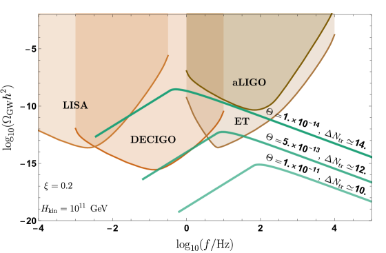
Figure 3: Comparison among the GW spectrum produced by the global cosmic string network during kinetic domination and the power-law integrated sensitivity curves of various GW experiments [65, 66]. Here we have assumed that the strings are immediately destroyed at the onset of radiation domination ($a_{\rm osc}=a_{\rm rad}$) and chosen fiducial values $H_{\rm kin}=10^{11}$ GeV and $\xi=0.2$. For this choice of parameters the backreaction of the cosmic string network is always small and the big bang nucleosynthesis constraint (2.4) is satisfied.

Ground-based interferometers such as LIGO [67], VIRGO [68] or the Einstein Telescope [69] are already sensitive to frequencies around $f\sim 100$ Hz, while space interferometers such as eLISA [70] or DECIGO [71] will be able to cover a $0.1$ mHz-$10$ Hz frequency window. The GW spectrum predicted by our mechanism is confronted with the power-law integrated sensitivity curves of these experiments in Fig. 3. As shown in this plot, a potentially observable window within the scope of future surveys can be easily found for not too large values of $H_{\rm kin}$ and relatively small heating efficiencies. It is important to notice that the produced spectrum is not restricted by CMB anisotropies. In particular, the production of GWs by Hubble-induced cosmic strings happens i) well-inside the horizon, ii) has a limited duration and iii) is restricted to highly energetic frequencies significantly exceeding those associated to the Hubble scale at decoupling, namely $3.4\times 10^{-19}\,{\rm Hz}<f_{\rm CMB}<2.1\times 10^{-17}\,{\rm Hz}$ [41]. The only restriction comes from its (integrated) contribution to the background energy density in Eq. (2.4). Note also that although our results are based on pure dimensional analysis and could therefore differ from the actual values by a few orders of magnitude (see for instance Ref. [13]) such uncertainty would not necessarily affect the observability of the model. In particular, a potential change in the amplitude of the spectrum could be easily compensated by a change on the number of e-folds spent in the rolling phase and on the duration of the kinetic dominated era.

It is interesting to compare our findings with previous results in the literature. On general grounds, our mechanism makes use of two basic ingredients: a non-minimal coupling to gravity and a period of kinetic domination. The fact that we are dealing with a Hubble-induced symmetry breaking pattern has far reaching consequences. First, the width of the strings in our scenario is proportional to the Hubble rate at the time of formation. Second, the temporal dependence in Eq. (4.3) forbids the appearance of an exact scaling regime. Third, the eventual restoration of the symmetry at the onset of radiation domination rescues the model from the limitations associated to (long-lived) non-scaling topological defects. All these properties are genuinely new, marking significant differences with the usual global string scenarios [73, 74, 75, 76]. This applies also to other studies in the literature involving also a kinetic dominated era [77, 78, 79]. Interestingly, a restoration mechanism similar to the one presented in this paper was used in Ref. [62] in a matter dominated era. Although the shape of the spectrum in the latest scenario shares some similarities with that in Fig. 3, the associated physics is completely different, in particular:

1. The energy density parameter $\Omega_{\rm GW}$ grows during kinetic domination rather than decreasing.

2. The knee in the spectrum in our scenario is not due to the transition from matter to radiation domination, but rather to the evolution of the $U(1)$ field from a rolling phase in which the energy density of the strings increases to a minimum phase in which the energy density of the strings decreases.

3. The spectral tilt at large frequencies depends in our case on the non-minimal coupling to gravity, rather than on the dimension of higher-dimensional operators.

4. Contrary to what happens in matter domination, the low frequency band of the spectrum is not always proportional to $k^{2}$, but rather depends on the detailed structure of the scalar potential.

Although the existence of a rolling phase is crucial for the GWs produced in our scenario to be within the observable band, its absence is also interesting by itself. In particular, the spectrum generated by an the minimum phase alone is always blue during kinetic domination, meaning that the leading contribution at the dominant high-frequency end $k_{\rm kin}$ can be easily constrained by the integrated bound in Eq. (2.4), namely

$$\Omega_{\rm GW}(k_{\rm kin})\sim 10^{-5}\,\Theta^{-1}\left(\frac{|\chi_{\rm min}(a_{\rm kin})|}{M_{\rm P}}\right)^{4}<10^{-6}\,.$$ (5.8)

This translates into a strong restriction on the presence of non-minimal couplings and on the duration of a kinetic dominated stage. Either the field stays sub-Planckian or the heating efficiency is high. In both cases, the GWs spectrum would never hit the observational band due to its strong blue tilt.

6 Conclusions

The free propagation of gravitational waves upon production makes them a perfect cosmological probe for retrieving information on energy scales and epochs that are hardly accessible by any other means. Violent processes such as inflation, (re)heating or phase transitions could naturally produce stochastic GW backgrounds within the reach of present and future GW interferometers.

In this paper we have considered the GW spectrum generated by a network of short-lived cosmic strings appearing in runaway quintessential inflation scenarios displaying a non-minimally coupled $U(1)$ spectator field. In this class of models, the Universe enters a kinetic-dominated regime soon after the end of inflation. During this unusual cosmological epoch the Ricci scalar turns negative, breaking spontaneously the $U(1)$ symmetry and triggering the formation of global cosmic strings. These topological defects emit GWs until the onset of radiation domination, where the Ricci scalar vanishes and the symmetry is restored. At this point, the strings decay, halting the GW production and leaving behind a GW background within the scope of near future observational campaigns. Interestingly, the spectrum displays some characteristic features that might allow to discriminate the proposed scenario from other mechanisms in the literature. On the one hand, its tilts are directly related to the non-minimal coupling to gravity and to the structure of the higher dimensional operators ensuring vacuum stability during kinetic domination. On the other hand, the amplitude at peak position is associated to the transition between a rolling phase associated with the initial stages of kinetic domination and a minimum phase in which the field tracks the minimum of the effective potential. In the event of a detection, these features provide a way of testing the structure of the scalar sector and the existence of non-minimal couplings to gravity, seeding some light on the underlying particle physics theory describing the early Universe. We have also argued that in the absence of a long rolling phase, the spectrum is only blue-tilted, leading to a strong restriction on non-minimal couplings to gravity and the duration of a kinetic dominated epoch.

The treatment presented in this paper is rather general and not linked to any particular realization of the quintessential inflationary paradigm or to the details of the entropy production process. Among other possibilities, our scenario could take place, for instance, in $\alpha$-attractor models [28, 80, 81, 82] or quantum gravity frameworks. [20, 25, 21]. The formalism could be additionally extended to accommodate a richer phenomenology, such as the generation of different short-lived topological defects or the creation of primordial black holes [83]. An interesting possibility along this line of thinking would be to identify the $U(1)$ charge with the baryonic number, while allowing for a small and explicit breaking of the $U(1)$ symmetry at large field values [14]. This framework could generate a non-vanishing global baryon asymmetry together with a correlated GW background, opening the possibility of testing baryogenesis with GWs. Determining the precise dynamics of this appealing scenario would most probably require the use of numerical simulations. We postpone the detailed analysis to a future work.

Appendix A Detailed computation of GW spectrum

In this appendix we give details on the computation of the integrated spectrum discussed in Sections 4.2 and 5 and plotted in Figs. 2 and 3. Our approach is based on two major approximations. First, we assume a sudden transition between the rolling and the minimum phases. Secondly, we slightly extrapolate the rolling phase solution beyond its regime of validity. Note, however, that none of these working assumptions has a significant impact on phenomenology. A more sophisticated analysis would merely provide more accurate restrictions on the model parameters, without significantly modifying the order of magnitude estimates presented here.

Our starting point is the integral in Eq. (4.10). With the same reasoning of that section this integral can be split into two parts, accounting for the amount of time spent by a given mode in the blue or red part of the spectrum. In this case, however, we have to consider that the solution changes at the transition between the rolling and the minimum phases, i.e. at $\tau=\tau_{\rm tr}$. This effect can be parametrized by a power-law peak emission

$$P_{\rm peak}(\tau)\sim\tau^{-\gamma(\tau)}\,,$$ (A.1)

with the time-dependent function $\gamma(\tau)$ interpolating between the constant peak exponents $\gamma_{\rm r}$ and $\gamma_{\rm m}$ associated to the rolling and minimum phases, cf. Table 1. Assuming, as explained above, a rapid transition between this two phases,

$$\gamma(\tau)=\gamma_{\rm r}\mathcal{S}(\tau_{\rm tr}-\tau)+\gamma_{\rm m}\mathcal{S}(\tau-\tau_{\rm tr})\,,$$ (A.2)

with $\mathcal{S}(\tau)$ the Heaviside step function, the integral in Eq. (4.10) can be written as

$$\Omega_{\rm GW}(\tau)\sim\frac{P_{\rm peak}(\tau_{\rm kin})}{\Theta}\left(\frac{a(\tau)}{a_{\rm rad}}\right)^{2}\left[\kappa^{\alpha}\int_{1}^{\kappa^{-1}}ds^{\prime}\left((s^{\prime})^{\alpha-2-\gamma(s^{\prime})}\right)+\kappa^{-\bar{\alpha}}\int_{x^{-1}}^{s(\tau)}ds^{\prime}\left((s^{\prime})^{-\bar{\alpha}-2-\gamma(s^{\prime})}\right)\right]\,,$$ (A.3)

where we have specialized to kinetic domination and defined dimensionless conformal times and momenta as in (4.18). This integral can be analytically performed to obtain

$$\Omega_{\rm GW}(\tau)\sim P_{\rm peak}(\tau_{\rm kin})\Theta^{-1}\left(\frac{a(\tau)}{a_{\rm rad}}\right)^{2}F(\kappa,s(\tau),s_{\rm tr})\,,$$ (A.4)

with the form factor $F$

$$F(\kappa,s(\tau),s_{\rm tr})=F_{+}(\kappa,s_{\rm tr})+F_{-}(\kappa,s(\tau),s_{\rm tr})$$ (A.5)

made of two pieces

$$F_{+}(\kappa,s_{\rm tr}) = \kappa^{\alpha}\begin{cases}\frac{1-\kappa^{\beta_{\rm r}-\alpha}}{\beta_{\rm r}-\alpha}&\quad\text{for}\quad s_{\rm tr}\,\kappa>1\\ \frac{1-s_{\rm tr}^{-\beta_{\rm r}+\alpha}}{\beta_{\rm r}-\alpha}&\quad\text{for}\quad s_{\rm tr}\,\kappa=1\\ \frac{s_{\rm tr}^{1-\beta_{\rm r}-\beta_{\rm m}}}{(\beta_{\rm m}-\alpha)(\alpha-\beta_{\rm r})}\left[s_{\rm tr}^{\alpha-1}(s_{\rm tr}^{\beta_{\rm m}}(\beta_{\rm m}-\alpha)-s_{\rm tr}^{\beta_{\rm r}}(\beta_{\rm r}-\alpha))\right.\\ \left.\qquad+s_{\rm tr}^{\beta_{\rm r}+\beta_{\rm m}-1}(\kappa^{\beta_{\rm m}-\alpha}(\beta_{\rm r}-\alpha)-(\beta_{\rm m}-\alpha))\right]&\quad\text{for}\quad s_{\rm tr}\,\kappa<1\end{cases}$$ (A.6)

$$F_{-}(\kappa,s(\tau),s_{\rm tr}) = \kappa^{-\bar{\alpha}}\begin{cases}\frac{s_{\rm tr}^{-\bar{\alpha}-\beta_{\rm m}-\beta_{\rm r}+1}}{(\bar{\alpha}+\beta_{\rm m})(\bar{\alpha}+\beta_{\rm r})}\left[s_{\rm tr}^{\beta_{\rm m}-1}(\bar{\alpha}+\beta_{\rm m})(-1+s_{\rm tr}^{\bar{\alpha}+\beta_{\rm r}}\kappa^{\bar{\alpha}+\beta_{\rm r}})\right.\\ \left.\qquad+(\bar{\alpha}+\beta_{\rm r})s_{\rm tr}^{\beta_{\rm r}-1}(1-s_{\rm tr}^{\bar{\alpha}+\beta_{\rm m}}s(\tau)^{-\bar{\alpha}-\beta_{\rm m}})\right]&\quad\text{for}\quad s_{\rm tr}\,\kappa>1\\ \frac{s_{\rm tr}^{-\bar{\alpha}-\beta_{\rm m}}-s(\tau)^{-\bar{\alpha}-\beta_{\rm m}}}{\bar{\alpha}+\beta_{\rm m}}&\quad\text{for}\quad s_{\rm tr}\,\kappa=1\\ \frac{\kappa^{\bar{\alpha}+\beta_{\rm m}}-s(\tau)^{-\bar{\alpha}-\beta_{\rm m}}}{\bar{\alpha}+\beta_{\rm m}}&\quad\text{for}\quad s_{\rm tr}\,\kappa<1\par\end{cases}$$ (A.7)

We have confronted this involved analytical result with the numerical integration of the spectrum using a smoother transition function between the rolling and minimum phases, finding a very good qualitative agreement. The main difference between the two approaches is the time needed for the field reach the minimum, being this one slightly larger in the sudden approximation.

References

- [1] Virgo, LIGO Scientific collaboration, B. P. Abbott et al., Observation of Gravitational Waves from a Binary Black Hole Merger, Phys. Rev. Lett. 116 (2016) 061102 [1602.03837].
- [2] Virgo, LIGO Scientific collaboration, B. P. Abbott et al., GW151226: Observation of Gravitational Waves from a 22-Solar-Mass Binary Black Hole Coalescence, Phys. Rev. Lett. 116 (2016) 241103 [1606.04855].
- [3] Virgo, LIGO Scientific collaboration, B. P. Abbott et al., GW170817: Observation of Gravitational Waves from a Binary Neutron Star Inspiral, Phys. Rev. Lett. 119 (2017) 161101 [1710.05832].
- [4] Virgo, Fermi-GBM, INTEGRAL, LIGO Scientific collaboration, B. P. Abbott et al., Gravitational Waves and Gamma-rays from a Binary Neutron Star Merger: GW170817 and GRB 170817A, Astrophys. J. 848 (2017) L13 [1710.05834].
- [5] A. A. Starobinsky, Spectrum of relict gravitational radiation and the early state of the universe, JETP Lett. 30 (1979) 682.
- [6] V. A. Rubakov, M. V. Sazhin and A. V. Veryaskin, Graviton Creation in the Inflationary Universe and the Grand Unification Scale, Phys. Lett. 115B (1982) 189.
- [7] J. Garcia-Bellido, D. G. Figueroa and A. Sastre, A Gravitational Wave Background from Reheating after Hybrid Inflation, Phys. Rev. D77 (2008) 043517 [0707.0839].
- [8] C. Grojean and G. Servant, Gravitational Waves from Phase Transitions at the Electroweak Scale and Beyond, Phys. Rev. D75 (2007) 043507 [hep-ph/0607107].
- [9] D. J. Weir, Gravitational waves from a first order electroweak phase transition: a brief review, Phil. Trans. Roy. Soc. Lond. A376 (2018) 20170126 [1705.01783].
- [10] A. Vilenkin and E. P. S. Shellard, Cosmic Strings and Other Topological Defects. Cambridge University Press, 2000.
- [11] E. J. Copeland and T. W. B. Kibble, Cosmic Strings and Superstrings, Proc. Roy. Soc. Lond. A466 (2010) 623 [0911.1345].
- [12] J.-F. Dufaux, D. G. Figueroa and J. Garcia-Bellido, Gravitational Waves from Abelian Gauge Fields and Cosmic Strings at Preheating, Phys. Rev. D82 (2010) 083518 [1006.0217].
- [13] D. G. Figueroa, M. Hindmarsh and J. Urrestilla, Exact Scale-Invariant Background of Gravitational Waves from Cosmic Defects, Phys. Rev. Lett. 110 (2013) 101302 [1212.5458].
- [14] D. Bettoni and J. Rubio, Quintessential Affleck-Dine baryogenesis with non-minimal couplings, Phys. Lett. B784 (2018) 122 [1805.02669].
- [15] J. Garcia-Bellido, J. Rubio, M. Shaposhnikov and D. Zenhausern, Higgs-Dilaton Cosmology: From the Early to the Late Universe, Phys. Rev. D84 (2011) 123504 [1107.2163].
- [16] G. K. Karananas and J. Rubio, On the geometrical interpretation of scale-invariant models of inflation, Phys. Lett. B761 (2016) 223 [1606.08848].
- [17] S. Casas, M. Pauly and J. Rubio, Higgs-dilaton cosmology: An inflation–dark-energy connection and forecasts for future galaxy surveys, Phys. Rev. D97 (2018) 043520 [1712.04956].
- [18] C. Wetterich, Cosmology and the Fate of Dilatation Symmetry, Nucl. Phys. B302 (1988) 668 [1711.03844].
- [19] C. Wetterich, The Cosmon model for an asymptotically vanishing time dependent cosmological ’constant’, Astron. Astrophys. 301 (1995) 321 [hep-th/9408025].
- [20] C. Wetterich, Inflation, quintessence, and the origin of mass, Nucl. Phys. B897 (2015) 111 [1408.0156].
- [21] J. Rubio and C. Wetterich, Emergent scale symmetry: Connecting inflation and dark energy, Phys. Rev. D96 (2017) 063509 [1705.00552].
- [22] P. J. E. Peebles and A. Vilenkin, Quintessential inflation, Phys. Rev. D59 (1999) 063505 [astro-ph/9810509].
- [23] B. Spokoiny, Deflationary universe scenario, Phys. Lett. B315 (1993) 40 [gr-qc/9306008].
- [24] P. Brax and J. Martin, Coupling quintessence to inflation in supergravity, Phys. Rev. D71 (2005) 063530 [astro-ph/0502069].
- [25] M. W. Hossain, R. Myrzakulov, M. Sami and E. N. Saridakis, Variable gravity: A suitable framework for quintessential inflation, Phys. Rev. D90 (2014) 023512 [1402.6661].
- [26] A. Agarwal, R. Myrzakulov, M. Sami and N. K. Singh, Quintessential inflation in a thawing realization, Phys. Lett. B770 (2017) 200 [1708.00156].
- [27] C.-Q. Geng, C.-C. Lee, M. Sami, E. N. Saridakis and A. A. Starobinsky, Observational constraints on successful model of quintessential Inflation, JCAP 1706 (2017) 011 [1705.01329].
- [28] K. Dimopoulos and C. Owen, Quintessential Inflation with -attractors, JCAP 1706 (2017) 027 [1703.00305].
- [29] R. D. Peccei, J. Sola and C. Wetterich, Adjusting the Cosmological Constant Dynamically: Cosmons and a New Force Weaker Than Gravity, Phys. Lett. B195 (1987) 183.
- [30] C. Wetterich, Variable gravity Universe, Phys. Rev. D89 (2014) 024005 [1308.1019].
- [31] S.-J. Wang, Quintessential Starobinsky inflation and swampland criteria, 1810.06445.
- [32] L. H. Ford, Gravitational Particle Creation and Inflation, Phys. Rev. D35 (1987) 2955.
- [33] T. Damour and A. Vilenkin, String theory and inflation, Phys. Rev. D53 (1996) 2981 [hep-th/9503149].
- [34] G. N. Felder, L. Kofman and A. D. Linde, Inflation and preheating in NO models, Phys. Rev. D60 (1999) 103505 [hep-ph/9903350].
- [35] B. Feng and M.-z. Li, Curvaton reheating in nonoscillatory inflationary models, Phys. Lett. B564 (2003) 169 [hep-ph/0212213].
- [36] J. C. Bueno Sanchez and K. Dimopoulos, Curvaton reheating allows TeV Hubble scale in NO inflation, JCAP 0711 (2007) 007 [0707.3967].
- [37] K. Dimopoulos and T. Markkanen, Non-minimal gravitational reheating during kination, JCAP 1806 (2018) 021 [1803.07399].
- [38] T. Nakama and J. Yokoyama, Reheating through the Higgs amplified by spinodal instabilities and gravitational creation of gravitons, 1803.07111.
- [39] V. Sahni, The Energy Density of Relic Gravity Waves From Inflation, Phys. Rev. D42 (1990) 453.
- [40] M. Maggiore, Gravitational wave experiments and early universe cosmology, Phys. Rept. 331 (2000) 283 [gr-qc/9909001].
- [41] C. Caprini and D. G. Figueroa, Cosmological Backgrounds of Gravitational Waves, Class. Quant. Grav. 35 (2018) 163001 [1801.04268].
- [42] C. Wetterich, Growing neutrinos and cosmological selection, Phys. Lett. B655 (2007) 201 [0706.4427].
- [43] L. Amendola, D. Bettoni, G. Domènech and A. R. Gomes, Doppelgänger dark energy: modified gravity with non-universal couplings after GW170817, JCAP 1806 (2018) 029 [1803.06368].
- [44] L. Amendola, M. Baldi and C. Wetterich, Quintessence cosmologies with a growing matter component, Phys. Rev. D78 (2008) 023015 [0706.3064].
- [45] N. D. Birrell and P. C. W. Davies, Quantum Fields in Curved Space, Cambridge Monographs on Mathematical Physics. Cambridge Univ. Press, Cambridge, UK, 1984, 10.1017/CBO9780511622632.
- [46] M. Fairbairn, K. Kainulainen, T. Markkanen and S. Nurmi, Despicable Dark Relics: generated by gravity with unconstrained masses, 1808.08236.
- [47] G. Alonso-Álvarez and J. Jaeckel, Lightish but clumpy: scalar dark matter from inflationary fluctuations, JCAP 1810 (2018) 022 [1807.09785].
- [48] Ya. B. Zeldovich, I. Yu. Kobzarev and L. B. Okun, Cosmological Consequences of the Spontaneous Breakdown of Discrete Symmetry, Zh. Eksp. Teor. Fiz. 67 (1974) 3.
- [49] T. W. B. Kibble, Topology of Cosmic Domains and Strings, J. Phys. A9 (1976) 1387.
- [50] M. B. Hindmarsh and T. W. B. Kibble, Cosmic strings, Rept. Prog. Phys. 58 (1995) 477 [hep-ph/9411342].
- [51] G. D. Moore, Intercommutation of U(1) global cosmic strings, 1604.02356.
- [52] M. Gorghetto, E. Hardy and G. Villadoro, Axions from Strings: the Attractive Solution, JHEP 07 (2018) 151 [1806.04677].
- [53] A. Vaquero, J. Redondo and J. Stadler, Early seeds of of axion miniclusters, 1809.09241.
- [54] T. Damour and A. Vilenkin, Gravitational wave bursts from cusps and kinks on cosmic strings, Phys. Rev. D64 (2001) 064008 [gr-qc/0104026].
- [55] X. Siemens, V. Mandic and J. Creighton, Gravitational wave stochastic background from cosmic (super)strings, Phys. Rev. Lett. 98 (2007) 111101 [astro-ph/0610920].
- [56] M. Kawasaki, K. Miyamoto and K. Nakayama, Cosmological Effects of Decaying Cosmic String Loops with TeV Scale Width, 1105.4383.
- [57] D. P. Bennett and F. R. Bouchet, Cosmic string evolution, Phys. Rev. Lett. 63 (1989) 2776.
- [58] B. Allen and E. P. S. Shellard, Cosmic string evolution: a numerical simulation, Phys. Rev. Lett. 64 (1990) 119.
- [59] J. J. Blanco-Pillado, K. D. Olum and B. Shlaer, Large parallel cosmic string simulations: New results on loop production, Phys. Rev. D83 (2011) 083514 [1101.5173].
- [60] C. Ringeval, M. Sakellariadou and F. Bouchet, Cosmological evolution of cosmic string loops, JCAP 0702 (2007) 023 [astro-ph/0511646].
- [61] L. M. Krauss, Gravitational waves from global phase transitions, Phys. Lett. B284 (1992) 229.
- [62] A. Kamada and M. Yamada, Gravitational wave signals from short-lived topological defects in the MSSM, JCAP 1510 (2015) 021 [1505.01167].
- [63] J. F. Dufaux, A. Bergman, G. N. Felder, L. Kofman and J.-P. Uzan, Theory and Numerics of Gravitational Waves from Preheating after Inflation, Phys. Rev. D76 (2007) 123517 [0707.0875].
- [64] A. Kamada and M. Yamada, Gravitational waves as a probe of the SUSY scale, Phys. Rev. D91 (2015) 063529 [1407.2882].
- [65] E. Thrane and J. D. Romano, Sensitivity curves for searches for gravitational-wave backgrounds, Phys. Rev. D88 (2013) 124032 [1310.5300].
- [66] M. Breitbach, J. Kopp, E. Madge, T. Opferkuch and P. Schwaller, Dark, Cold, and Noisy: Constraining Secluded Hidden Sectors with Gravitational Waves, 1811.11175.
- [67] https://dcc.ligo.org/.
- [68] http://www.virgo-gw.eu/.
- [69] http://www.et-gw.eu.
- [70] http://lisa.nasa.gov/.
- [71] http://tamago.mtk.nao.ac.jp/decigo/index_E.html.
- [72] J. Yokoyama, Natural Way Out of the Conflict Between Cosmic Strings and Inflation, Phys. Lett. B212 (1988) 273.
- [73] C. Hagmann and P. Sikivie, Computer simulations of the motion and decay of global strings, Nucl. Phys. B363 (1991) 247.
- [74] M. Yamaguchi, M. Kawasaki and J. Yokoyama, Evolution of axionic strings and spectrum of axions radiated from them, Phys. Rev. Lett. 82 (1999) 4578 [hep-ph/9811311].
- [75] M. Yamaguchi, Scaling property of the global string in the radiation dominated universe, Phys. Rev. D60 (1999) 103511 [hep-ph/9907506].
- [76] M. Yamaguchi, J. Yokoyama and M. Kawasaki, Evolution of a global string network in a matter dominated universe, Phys. Rev. D61 (2000) 061301 [hep-ph/9910352].
- [77] Y. Cui, M. Lewicki, D. E. Morrissey and J. D. Wells, Cosmic Archaeology with Gravitational Waves from Cosmic Strings, Phys. Rev. D97 (2018) 123505 [1711.03104].
- [78] Y. Cui, M. Lewicki, D. E. Morrissey and J. D. Wells, Probing the pre-BBN universe with gravitational waves from cosmic strings, 1808.08968.
- [79] M. Artymowski, O. Czerwinska, Z. Lalak and M. Lewicki, Gravitational wave signals and cosmological consequences of gravitational reheating, JCAP 1804 (2018) 046 [1711.08473].
- [80] K. Dimopoulos, L. Donaldson Wood and C. Owen, Instant preheating in quintessential inflation with -attractors, Phys. Rev. D97 (2018) 063525 [1712.01760].
- [81] Y. Akrami, R. Kallosh, A. Linde and V. Vardanyan, Dark energy, -attractors, and large-scale structure surveys, JCAP 1806 (2018) 041 [1712.09693].
- [82] C. Garcia-Garcia, E. V. Linder, P. Ruiz-Lapuente and M. Zumalacarregui, Dark energy from -attractors: phenomenology and observational constraints, JCAP 1808 (2018) 022 [1803.00661].
- [83] L. Amendola, J. Rubio and C. Wetterich, Primordial black holes from fifth forces, Phys. Rev. D97 (2018) 081302 [1711.09915].