Initial-state-dependent thermalization in open qubits

Abstract

We study, from a thermodynamic perspective, the equilibrium states of a qubit interacting with an arbitrary environment of dimension $N\gg 2$. We show that even in presence of memory about the initial state, in some cases the qubit can be considered in a thermal state characterized by an entanglement Hamiltonian, which encodes the effects of the environment, and an initial-state-dependent entanglement temperature that measures the degree of entanglement generated between the system and its environment. Geometrical aspects of the thermal states are studied, and the results are confirmed for the concrete case of the Quantum Walk on the Line.

I Introduction

Quantum thermodynamics tries to account for the emergence, from the principles of Quantum Mechanics, of the thermodynamic behavior observed in macroscopic systems. This is not an easy task, since the unitary evolution of isolated quantum systems implies that the expected values of the corresponding physical quantities oscillate in time, and, as a consequence, the system is in general out of equilibrium Schulman . For a general review of this problem see Ref.Gemmer , and more recent discussions can be found in Refs.Goold ; Parrondo .

Recent theoretical work has considered the Eigenstate Thermalization Hypothesis, showing that quantum systems can indeed thermalize Polkovnicov . This hypothesis provides a framework connecting microscopic models and macroscopic phenomena, based on the notion of highly entangled quantum states. The role of quantum entanglement in the emergence of statistical mechanics in the quantum regime has been experimentally studied in Ref.Kaufman . This work shows that the entanglement entropy can be measured, playing a similar role as that of the thermal entropy in the classical thermalization processes. This validates the use of Statistical Physics for the measurement of local observables.

When we consider open quantum systems, we observe that in some cases the interaction with the environment may lead the system to an equilibrium state, despite the unitarity of the global dynamics. Although in general it is not an equilibrium stricto sensu, but rather a situation in which the system spends most of the time in the neighborhood of an average state, an attempt to conciliate thermodynamics with such kind of systems is therefore possible Romanelli1 ; Romanelli2 ; Novotny ; schliemann . In particular, it has been proved that a large energy-level occupation of the environment in the initial state establishes strong bounds to the distance between the reduced state of the subsystem and its corresponding time-average, which assures equilibration if the mentioned condition is satisfied Linden . Moreover, the canonical typicallity of reduced states of bipartite quantum systems has been proved, showing the ubiquity of the thermal behavior, even at the nanoscale Goldstein , Popescu .

In this context, we explore the equilibrium states of an open qubit, which, due to interaction with the environment, evolves to an initial-state-dependent equilibrium state. We find that in some cases, this dependence can be factorized in such a way that the reduced density operator (RDO) adopts the form of thermal state for some fixed operator that we call entanglement Hamiltonian, which depends on the relevant parameters of the global dynamics. Meanwhile, the corresponding entanglement temperature encloses the dependence on the initial state and can be interpreted as a measure of the entanglement generated during the process.

This paper is organized as follows. In section II, we introduce the concepts of entanglement Hamiltonian and entanglement temperature, notions that will allow us to define the thermal states in a proper way. Then, we explore some of their properties and find a property that allows to identify which of the asymptotically equilibrated initial-state-dependent reduced operators correspond to thermal states. In section III, we study this class of thermal states from a geometric perspective, finding their location on the Bloch sphere. In section IV we find the thermal states associated to the chirality degrees of freedom for a Quantum Walk on the Line. Finally, some remarks and perspectives are discussed in section V.

II RDO and thermal states

Let us consider an isolated bipartite quantum system composed of a qubit $S$ in thermal contact with an arbitrary environment $E$, so that the state space for the composed system is

$$\mathcal{H}=\mathcal{H}_{{}_{E}}\otimes\mathcal{H}_{{}_{S}}.$$ (1)

Let us suppose there is no initial correlation between the systems, so the initial state is a product state, that can be written as

$$|\Psi(0)\rangle=\sum_{n}C_{n}|n\rangle\otimes|\phi_{0}\rangle,$$ (2)

with

$$|\phi_{0}\rangle={\cos\frac{\gamma}{2}|+\rangle+e^{i\varphi}\sin\frac{\gamma}{2}|-\rangle},$$ (3)

where

• $\{|+\rangle,|-\rangle\}$ and $\{{|n\rangle}\}$ are some orthonormal bases in $\mathcal{H}_{{}_{S}}$ and $\mathcal{H}_{{}_{E}}$ respectively,

• $\gamma$ and $\varphi$ define the point over the Bloch sphere associated to the initial state of the qubit,

• $\{C_{n}\}$ are the amplitudes that define the initial occupation of the bath and satisfy the normalization condition $\sum_{n}|C_{n}|^{2}=1$.

If the system equilibrates on average via interaction with the environment, the equilibrium state is described by the time-averaged RDO Nielsen

$$\begin{split}\overline{\rho_{{}_{S}}}(\{C_{n}\},\gamma,\varphi)&=\langle\rho_{{}_{S}}(t,\{C_{n}\},\gamma,\varphi)\rangle_{t}\\ &=\lim_{\tau\to\infty}\frac{1}{\tau}\int_{0}^{\tau}\rho_{{}_{S}}(t,\{C_{n}\},\gamma,\varphi)dt,\\ \end{split}$$ (4)

where $\rho_{{}_{S}}=tr_{{}_{E}}\rho_{{}_{SE}}=tr_{{}_{E}}|\Psi\rangle\langle\Psi|$. Without loss of generality, $\overline{\rho_{{}_{S}}}$ can be written as

$$\overline{\rho_{{}_{S}}}(\{C_{n}\},\gamma,\varphi)=\begin{pmatrix}{\dfrac{1}{2}+a}&{b}\\ {b^{*}}&{\dfrac{1}{2}-a}\end{pmatrix}.$$ (5)

where $a$ and $b$ depend on the initial conditions $\{C_{n}\}$, $\gamma$ and $\varphi$. In a few interesting cases, the limit (4) coincides with the asymptotic limit of the RDO as $t\to\infty$ Romanelli1 . But in most of cases, the notion of equilibration on average (or in another relevant sense) is necessary since, due to the Quantum Recurrence Theorem, in general the asymptotic limit of local operators does not exist Bocchieri .

Now we will investigate if, despite the initial state dependence, there are situations in which the system can be considered in thermal equilibrium, i.e., if there exists an operator $H_{ent}$, defined on $\mathcal{H_{S}}$, and a real number $\beta$ such that $\overline{\rho_{{}_{S}}}$ adopts the form

$$\overline{\rho_{{}_{S}}}=\dfrac{e^{-\beta H_{ent}}}{tr(e^{-\beta H_{ent}})}.$$ (6)

Note that the operator $H_{ent}$ may not coincide with the free Hamiltonian, due to environment effects. The Hamiltonian $H_{ent}$ that governs the dynamics in the asymptotic regime cannot (or, at least, should not) be initial-state-dependent. So we will center our attention in investigating if it is possible to factorize the exponent in Eq.(6) in such a way that the initial state dependence appears as a scalar factor, that we will interpret as the entanglement temperature, multiplied by a initial-state-independent operator, which plays the role of an entanglement Hamiltonian. When such a factorization is possible, the entanglement Hamiltonian will be well-defined except for an additive multiple of the identity (related to an irrelevant energy shift), and a multiplicative factor that represents an also irrelevant change of scale in the temperature. Then, we will have that systems in different initial states, governed by the same entanglement Hamiltonian, will thermalize at different inverse entanglement temperatures $\beta$.
As we will see, the aforementioned factorization is only possible for a small set of initial-state-dependent RDOs, that we will call initial-state-dependent thermal states.

The parameter $T_{ent}=1/\beta$ is, a priori, not related to the thermodynamic temperature and will be denoted entanglement temperature. It is easy to show the following properties of the thermal states defined in Eq.(6):

• If ${\lambda_{j}}$ are the natural populations of the system S and ${E_{j}}$ its energy eigenvalues, then $\delta Q=T_{ent}dS_{vN}$, where $\delta Q=\sum_{j}E_{j}d\lambda_{j}$ is the heat exchanged with the environment, and $S_{vN}=-\sum_{j}\lambda_{j}\log{\lambda_{j}}$ is the von Neumann entropy Gemmer . This result, valid for infinitesimal transitions between thermal states emphasizes the similarity between entanglement thermodynamics and classical thermodynamics.

• $T_{ent}=0$ for pure reduced states and $T_{ent}=\infty$ for the maximally mixed state. In fact, $T_{ent}$ is a growing function of $S_{vN}$, so the entanglement temperature is a measure of the entanglement generated between the system and its environment.

We note that the positivity of the RDO $\overline{\rho_{{}_{S}}}$, implies that it is always possible to express it in the exponential form of Eq.(6), so, a priori, every reduced state is, potentially, a thermal state. In fact, there is an infinite number of ways of selecting $\beta$ and $H_{ent}$ for a given state, so the system can be considered in equilibrium at any temperature, depending on the choice of $H_{ent}$.

In order to obtain an explicit condition for such factorization, let us consider the basis $\{|\psi^{+}\rangle$, $|\psi^{-}\rangle\}$ that diagonalizes $\overline{\rho_{{}_{S}}}$. The functional relation between $\overline{\rho_{{}_{S}}}$ and $H_{ent}$ implies that the latter will also have a diagonal expression in that basis. If we denote by $\{\varepsilon$, $-\varepsilon\}$ the eigenvalues of $H_{ent}$, and by $\{\lambda^{+}$,$\lambda^{-}\}$ the corresponding natural populations, we have

$$H_{ent}^{(diag)}=\begin{pmatrix}{\varepsilon}&{0}\\ {0}&{-\varepsilon}\end{pmatrix},\;\;\overline{\rho_{{}_{S}}}^{(diag)}=\begin{pmatrix}{\lambda^{+}}&{0}\\ {0}&{\lambda^{-}}\end{pmatrix}.$$ (7)

Now, observe that if ${\overline{\rho_{{}_{S}}}}^{(diag)}$ can be obtained from $\overline{\rho_{{}_{S}}}$ through the change of basis

$${\overline{\rho_{{}_{S}}}}^{(diag)}=Q^{{\dagger}}\overline{\rho_{{}_{S}}}Q,$$ (8)

then, via the inverse transformation, we can find the explicit form of $H_{ent}$ in the base $\{|+\rangle,|-\rangle\}$:

$$H_{ent}=QH_{ent}^{(diag)}Q^{{\dagger}}.$$ (9)

Let us implement the described procedure. We first find the eigenvalues of (5):

$$\lambda^{\pm}=\dfrac{1}{2}\pm\sqrt{a^{2}+|b|^{2}},$$ (10)

and the corresponding eigenvectors:

$$|\psi^{\pm}\rangle=\begin{pmatrix}{\psi_{1}^{\pm}}\\ \vspace{0.2cm}{\psi_{2}^{\pm}}\end{pmatrix},$$ (11)

where

$$\begin{cases}\psi_{1}^{\pm}=\dfrac{|{b}|\left(a\pm\sqrt{a^{2}+|{b}|^{2}}\right)}{b^{*}\sqrt{\left(a\pm\sqrt{a^{2}+|{b}|^{2}}\right)^{2}+|{b}|^{2}}},\\ \vspace{0.2cm}\psi_{2}^{\pm}=\dfrac{|{b}|}{\sqrt{\left({a\pm\sqrt{a^{2}+|{b}|^{2}}}\right)^{2}+|{b}|^{2}}}.\end{cases}$$ (12)

So the change of basis matrix that simultaneously diagonalizes the operators $\overline{\rho_{{}_{S}}}$ and $H_{ent}$ is

$$Q=\begin{pmatrix}{\psi_{1}^{+}}&{\psi_{1}^{-}}\vspace{0.2cm}\\ {\psi_{2}^{+}}&{\psi_{2}^{-}}\end{pmatrix}.\$$ (13)

Now, employing Eq.(9) we obtain the following expression for the entanglement Hamiltonian in the base $\{|+\rangle,|-\rangle\}$:

$$H_{ent}=QH^{(diag)}_{ent}Q^{{\dagger}}=\varepsilon\begin{pmatrix}{\dfrac{a}{\sqrt{a^{2}+|{b}|^{2}}}}&{\dfrac{b}{\sqrt{a^{2}+|{b}|^{2}}}}\\ {\dfrac{b^{*}}{\sqrt{a^{2}+|{b}|^{2}}}}&{\dfrac{-a}{\sqrt{a^{2}+|{b}|^{2}}}}\end{pmatrix}.$$ (14)

Equation (14) shows an evident dependence on the initial state through the coefficients $a$ and $b$. We then conclude that, in general, it is not possible to express the equilibrium state in the form of a thermal state (Eq.(6)) with an universal, i.e. valid for any initial condition, entanglement Hamiltonian. However, there is a particular relation between the parameters $a$ and $b$ that makes $H_{ent}$ independent of the initial state. Note that, if a constant $\kappa$ independent of $\gamma$, $\varphi$ and $\{C_{n}\}$ can be found such that $b=\kappa a$, and taking into account that $a\in R$, we have

$$H_{ent}=\dfrac{\varepsilon}{\sqrt{1+|{\kappa}|^{2}}}\begin{pmatrix}{1}&{\kappa}\\ {\kappa^{*}}&{-1}\end{pmatrix}.$$ (15)

Reciprocally, if Eq.(14) is independent of the initial state, we can write

$$\varepsilon\begin{pmatrix}{\dfrac{a}{\sqrt{a^{2}+|{b}|^{2}}}}&{\dfrac{b}{\sqrt{a^{2}+|{b}|^{2}}}}\\ {\dfrac{b^{*}}{\sqrt{a^{2}+|{b}|^{2}}}}&{\dfrac{-a}{\sqrt{a^{2}+|{b}|^{2}}}}\end{pmatrix}=\begin{pmatrix}{\eta_{1}}&{\eta_{2}}\\ {\eta^{*}_{2}}&{\eta_{1}}\end{pmatrix},$$ (16)

where $\eta_{1}$ and $\eta_{2}$ do not depend on $\{C_{n}\}$, $\gamma$, $\varphi$. Then, we have

$$b/a=\dfrac{\dfrac{b}{\sqrt{a^{2}+|{b}|^{2}}}}{\dfrac{a}{\sqrt{a^{2}+|{b}|^{2}}}}=\dfrac{\eta_{2}}{\eta_{1}}=\kappa,$$ (17)

where $\kappa$ is a constant.

The previous analysis can be summarized in the following proposition:

Proposition 1

A time-averaged RDO of the type of Eq.(5) describing an equilibrated qubit is an initial-state-dependent thermal state if, and only if there exists a set of initial conditions such that:

$$b(\{C_{n}\},\gamma,\varphi)=\kappa a(\{C_{n}\},\gamma,\varphi),$$ (18)

where $\kappa\in C$ is a constant independent of the initial state. In that case, the entanglement Hamiltonian in the basis $\{|+\rangle,|-\rangle\}$ takes the form

$$H_{ent}=\dfrac{\varepsilon}{\sqrt{1+|\kappa|^{2}}}\begin{pmatrix}{1}&{\kappa}\\ {\kappa^{*}}&{-1}\end{pmatrix},$$ (19)

except for an arbitrary multiplicative factor, or an additive multiple of the identity, which do not lead to relevant physical consequences.

III The role of the entanglement Hamiltonian: geometry of thermal states

In general, we expect that the dimensionless quantity $\kappa$ that defines the entanglement Hamiltonian can be constructed from the parameters involved in the global Hamiltonian that characterize the system and its interaction with the environment, such as coupling constants or characteristic frequencies.
In particular, a simple consequence of the restriction $b(C_{n},\gamma,\varphi)=\kappa a(C_{n},\gamma,\varphi)$ arises by analyzing the location of the thermal states on the Bloch sphere.

Because of Proposition (1), we know that the RDO of an initial-state-dependent thermal state can be written in the form

$$\overline{\rho_{{}_{S}}}=\begin{pmatrix}{\dfrac{1}{2}+a}&{\kappa a}\\ {\kappa^{*}a}&{\dfrac{1}{2}-a}\end{pmatrix},$$ (20)

where the dependence on the initial state is totally included in $a$. On the other hand, in terms of the Bloch vector components, $\vec{B}=(B_{1},B_{2},B_{3})$, representing the state, the expression for this operator is Nielsen

$$\overline{\rho_{{}_{S}}}=\dfrac{1}{2}\begin{pmatrix}{1+B_{3}}&{B_{1}-iB_{2}}\\ {B_{1}+iB_{2}}&{1-B_{3}}\end{pmatrix}.$$ (21)

Comparing both expressions we have that

$$\vec{B}=2a\vec{v},$$ (22)

with

$$\vec{v}=\left({\rm{Re}}(\kappa),-{\rm{Im}}(\kappa),1\right),$$ (23)

where ${\rm{Re}}(\kappa)$ and ${\rm{Im}}(\kappa)$ denote the real and imaginary parts of $\kappa$. Note that the direction of the Bloch vector is completely defined by the quantity $\kappa$, while the initial state only plays a role in fixing its modulus. Given that $\kappa$ only depends on the relevant parameters involved in the global dynamics, which are fixed in advance, we conclude that the entanglement Hamiltonian fixes, through the parameter $\kappa$, the diameter of the Bloch sphere that corresponds to the locus of the thermal states. In fact, observe that the entanglement Hamiltonian (15) can be expressed as

$$H_{ent}=\frac{\varepsilon}{\sqrt{1+|\kappa|^{2}}}\left(\vec{v}.\vec{\sigma}\right),$$ (24)

where $\vec{\sigma}=\left(\sigma_{x},\sigma_{y},\sigma_{z}\right)$ is the vector whose components are the Pauli matrices. So the vector $\vec{v}$ can be interpreted as an effective magnetic field that selects the privileged direction along which the spin will relax due to interaction with the environment.

As an example, let us analyze the case in which $\rho_{{}_{S}}$ possesses an asymptotic limit $\rho_{{}_{S}}^{\infty}$ that admits a Kraus representation in terms of orthogonal projectors, i.e.

$$\rho_{{}_{S}}^{\infty}=\sum_{j}M_{j}\rho_{{}_{S}}(0)M_{j}^{\dagger},$$ (25)

where $M_{j}=|\psi_{j}\rangle\langle\psi_{j}|$ and $\langle\psi_{i}|\psi_{j}\rangle=\delta_{ij}$, $j=1,2$. This could seem rather artificial, but in the following section we provide an example of a relevant quantum system verifying such conditions.
It is clear that in this case, the time-averaged RDO, $\overline{\rho_{{}_{S}}}$, coincides with the asymptotic limit, $\rho_{{}_{S}}^{\infty}$. If $\rho_{{}_{S}}(0)=|\phi_{0}\rangle\langle\phi_{0}|$ then

$$\overline{\rho{{}_{S}}}|\psi_{1,2}\rangle=|\langle\phi_{0}|\psi_{1,2}\rangle|^{2}|\psi_{1,2}\rangle,$$ (26)

so the kets $|\psi_{1,2}\rangle$ are eigenvectors of $\overline{\rho_{{}_{S}}}$, with corresponding eigenvalues $|{\langle\phi_{0}|\psi_{1,2}\rangle}|^{2}$, so it is clear that

$$|\psi_{1,2}\rangle=|\psi^{\pm}\rangle,$$ (27)

where $|\psi^{\pm}\rangle$ are given by (11). Using Eqs. (26) and (27) we have that

$$\lambda^{+}-\lambda^{-}=|\langle\phi_{0}|\psi^{+}\rangle|^{2}-|\langle\phi_{0}|\psi^{-}\rangle|^{2},$$ (28)

and using Eqs.(10), (12), (18) and (28), it is straightforward to show that

$$a=\dfrac{\cos\alpha}{2\sqrt{1+|{\kappa}|^{2}}},$$ (29)

where

$$\cos\alpha\equiv\frac{{\rm{Re}}(\kappa)\sin\gamma\cos\varphi-{\rm{Im}}(\kappa)\sin\gamma\sin\varphi+\cos\gamma}{\sqrt{1+|{\kappa}|^{2}}}.$$ (30)

It is interesting to point out that Eq.(30) can be expressed as

$$\cos\alpha=\vec{B_{0}}.\frac{\vec{v}}{|\vec{v}|},$$ (31)

where $\vec{B}_{0}=(\sin\gamma\cos\varphi,\sin\gamma\sin\varphi,\cos\gamma)$ is the initial Bloch vector. From Eq.(31) we see that $\alpha$ is the angle between $\vec{B}_{0}$ and $\vec{v}$. Finally, the expression for $\overline{\rho_{{}_{S}}}$ is

$$\overline{\rho_{{}_{S}}}=\frac{1}{2}\begin{pmatrix}{1+\dfrac{\cos\alpha}{\sqrt{1+|{\kappa}|^{2}}}}&{{\dfrac{\kappa\cos{\alpha}}{\sqrt{1+|{\kappa}|^{2}}}}}\\ {{\dfrac{\kappa^{*}\cos\alpha}{\sqrt{1+|{\kappa}|^{2}}}}}&{1-\dfrac{\cos\alpha}{\sqrt{1+|{\kappa}|^{2}}}}\end{pmatrix}.$$ (32)

The entanglement temperature can be obtained from the eigenvalues of $\overline{\rho_{{}_{S}}}$, so we can construct the isotemperature contour lines on the Bloch sphere (see Fig.1) considering

$$T_{ent}=\dfrac{2\varepsilon}{\log\left(\dfrac{\lambda^{+}}{\lambda^{-}}\right)}=\dfrac{-\varepsilon}{\log\left[\tan\alpha/2\right]},$$ (33)

which implies that these lines correspond to constant values of the angle $\alpha$. Expressing this condition in Cartesian coordinates, $x=\sin\gamma\cos\varphi$, $y=\sin\gamma\sin\varphi$, $z=\cos\gamma$, we obtain

$${\rm{Re}}(\kappa)x-{\rm{Im}}(\kappa)y+z=\sqrt{1+|{\kappa}|^{2}}\cos{\alpha}.$$ (34)

Eq.(34) represents a family of parallel planes, which are orthogonal to the vector $\vec{v}$ (see Fig.1). The intersection of these planes with the Bloch surface produces a family of concentric circumferences, each of which characterized by a specific value of asymptotic entanglement temperature. For the particular initial states on the equatorial plane ${\rm{Re}}(\kappa)x-{\rm{Im}}(\kappa)y+z=0$ ($\alpha=\pi/2$), the matrix expression for the RDO adopts the maximally mixed form

$$\overline{\rho_{{}_{S}}}=\frac{1}{2}\begin{pmatrix}{1}&{0}\\ {0}&{1}\end{pmatrix}.$$ (35)

As we move over on the northern hemisphere’s surface towards the pole defined by the vector $\vec{v}$ ($\alpha=0$), the temperature decreases from $T_{ent}\rightarrow+\infty$ near the equatorial plane, reaching its minimum value $T_{ent}=0$ at the North pole in Fig.1. Similarly, as we move towards the South pole, defined by the vector $\vec{v}$ ($\alpha=\pi$), the entanglement temperature increases from $T_{ent}=-\infty$ at the equator to $T_{ent}=0$ at the pole.

In what refers to the location of a particular thermal state on the Bloch sphere, it is clear that its Bloch vector is orthogonal to the level plots of the entanglement temperature. The distance between the center of the sphere $\vec{O}=(0,0,0)$ and the plane $\pi_{\alpha_{0}}$ of Eq.(34) is given by

$$d(\vec{O},\pi_{\alpha_{0}})=\frac{|{\sqrt{1+|{\kappa}|^{2}}\cos\alpha_{0}}|}{\sqrt{1+\kappa^{2}}}=|{\cos\alpha_{0}}|.$$ (36)

While the norm of $\vec{B}$, Eq.(22) is

$$|\vec{B}|=2|a|\sqrt{1+\kappa^{2}},$$ (37)

where $a$ is given by Eq.(29). Thus, we have

$$\begin{split}|\vec{B}|=|{\cos\alpha_{0}}|=d(\vec{O},\pi_{\alpha_{0}}).\end{split}$$ (38)

So, we conclude that the thermal state is located at the center of the corresponding entanglement temperature level plot, see Fig.1.

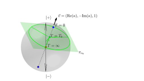
Figure 1: (Color online) Level plots of the entanglement temperature over the Bloch sphere for a time-averaged RDO whose Kraus operators are orthogonal projectors. The temperature $T_{0}$ (green point) corresponds to the asymptotic limit of all initial pure states located on the intersection of the plane ${\rm{Re}}(\kappa)x-{\rm{Im}}(\kappa)y+z=\sqrt{1+|\vec{\kappa}|^{2}}\cos\alpha_{0}$ with the sphere, as shown by the arrows. Also represented are the minimum temperature states $T=0$ (blue points), and the $T=\infty$ state (red).

IV Example: Thermalization in the Quantum Walk on the line

The Quantum Walk (QW) is the quantum analog of the classical random walk, and it has been studied from multiple perspectives given the wealth of its applications travaglione , Renato , Grover . In particular, the relation between the asymptotic coin-position entanglement and the initial conditions of the QW has been investigated by several authors Nayak ; Carneiro ; Abal ; Annabestani ; Omar ; Pathak ; Petulante ; Venegas ; Endrejat ; Ellinas1 ; Ellinas2 ; Maloyer . In this context, we shall emphasize the thermodynamical aspects, as an application of the previous section. We begin by noting that the mathematical structure behind the QW allows us to consider the chirality degrees of freedom as a qubit $S$, described by a two-dimensional Hilbert space $\mathcal{H}_{S}$, in interaction with a thermal bath, represented by the walker’s Hilbert space $\mathcal{H}_{n}$. Then, we will show that for an adequate initial state of the bath, the asymptotic reduced state of the qubit is an initial-state-dependent thermal state, which will allow to illustrate the results obtained in the previous section and, in this context, give a physical interpretation to the parameter $\kappa$.

First, we briefly review the QW dynamical equations in discrete time. The system evolves under successive applications of the evolution operator $U$, acting on $\mathcal{H}_{n}\otimes\mathcal{H}_{S}$

$$U=\mathcal{T}(I_{n}\otimes U_{\theta}),$$ (39)

where $U_{\theta}$ is an unitary evolution operator in 2D, describing the quantum coin and parameterized by the coin bias parameter $\theta$,

$$U_{\theta}=\begin{pmatrix}{\cos\theta}&{\sin\theta}\\ {\sin\theta}&{-\cos\theta}\end{pmatrix}.$$ (40)

This particular parameterization of $U_{\theta}$ is sufficient to display all the possible evolutions of the QW.

In Eq.(39) $\mathcal{T}$ is the conditional translation operator

$$\mathcal{T}=\sum_{n}|n+1\rangle\langle n|\otimes|+\rangle\langle+|+\sum_{n}|n-1\rangle\langle n|\otimes|-\rangle\langle-|,$$ (41)

and $I_{n}$ is the identity operator in $\mathcal{H}_{n}$.

Any pure initial state can be expressed as

$$|\psi(0)\rangle=\sum_{n}|n\rangle\otimes[d_{n}(0)|+\rangle+e_{n}(0)|-\rangle],$$ (42)

where $\{|n\rangle\}$, $n\in Z$ is an orthonormal basis of $\mathcal{H}_{n}$ associated to the classical positions of the walker (integer points on the line), $\{|+\rangle,|-\rangle\}$ are the chirality eigenstates in $\mathcal{H}_{S}$, and $d_{n}(0)$, $e_{n}(0)$ satisfy the normalization condition $\sum_{n}\left[|d_{n}(0)|^{2}+|e_{n}(0)|^{2}\right]=1$. After $t$ applications of $U$, the QW state is

$$|\psi(t)\rangle=U^{t}|\psi(0)\rangle=\sum_{n}|n\rangle\otimes[d_{n}(t)|+\rangle+e_{n}(t)|-\rangle].$$ (43)

For an infinite line, it is a well known fact that the coin system reaches an equilibrium state as $t\rightarrow\infty$ Nayak . The reduced state of the coin adopts the characteristic form of Eq. (5), where the expression for $b$ in terms of the wave function coefficients is

$$b\equiv\begin{array}[]{c}\lim_{t\rightarrow\infty}\sum_{n=-\infty}^{\infty}d_{n}(t)e_{n}^{\ast}(t)\\ \end{array}.\,$$ (44)

In Ref. Romanelli1 it is shown that the entries of the coin RDO defined in Eq. (5), for an arbitrary initial state, satisfy the relation

$$a(\theta,\gamma,\varphi)=\frac{{\rm{Re}}(b(\theta,\gamma,\varphi))}{\tan\theta}.\,$$ (45)

On the other hand, Proposition (1) shows that an initial-state-dependent thermal state must verify that

$$\frac{b(\theta,\gamma,\varphi)}{a(\theta,\gamma,\varphi)}=\kappa(\theta),$$ (46)

since $\kappa$ must be independent of the initial state.

Given that $b={\rm{Re}}(b)+i{\rm{Im}}(b)$ and using Eqs. (45) and  (46), we find that the thermal state is guaranteed if

$$\left[1+\frac{i{\rm{Im}}(b(\theta,\gamma,\varphi))}{{\rm{Re}}(b(\theta,\gamma,\varphi))}\right]\tan\theta=\kappa(\theta),$$ (47)

condition that is satisfied if the real and imaginary parts of $b$ are proportional to each other, with a proportionality constant function of only $\theta$.

As a first example, we assume that the initial state of the walker is sharply localized at the origin, with arbitrary chirality. Thus

$$|\psi(0)\rangle=|0\rangle\otimes|\phi_{0}\rangle,$$ (48)

where $\phi_{0}$ was defined in Eq.(3). This situation was studied in Ref.Romanelli1 , where an explicit expression for $b$ was obtained (Eq. (16) of that reference), for a coin toss bias parameter $\theta=\pi/4$. In our present nomenclature

$$b=\frac{1}{2}(1-\frac{1}{\sqrt{2}})\left[\cos\gamma\text{ }+\sin\gamma\text{ }(\cos\varphi+i\sqrt{2}\sin\varphi)\right].$$ (49)

In this case, from the considerations below Eq.(47), it is clear that $\kappa$ depends on the initial state, so the equilibrium state is not an initial-state-dependent thermal state.

As a second case, we consider strongly non-localized initial states of the walker. One way of implementing this initial condition was studied in Ref.Orthey , where the following initial state is considered

$$d_{n}(0)=\frac{e^{\frac{-n^{2}}{4\xi^{2}}}}{\sqrt[4]{2\pi\xi^{2}}}\cos(\gamma/2),$$ (50)

$$e_{n}(0)=\frac{e^{\frac{-n^{2}}{4\xi^{2}}}}{\sqrt[4]{2\pi\xi^{2}}}\sin(\gamma/2)e^{i\varphi},$$ (51)

which corresponds to an initially Gaussian distributed walker with the restriction $\xi\gg 1$. We obtained the relation between $b$ and the initial condition using directly Eqs.(19) and (29) of Ref.Orthey in the case $\theta=\pi/4$,

$$b=\frac{1}{4}(\cos\gamma\text{ }+\sin\gamma\cos\varphi).$$ (52)

Following the same procedure, we have generalized this last equation for all $\theta$. The result is

$$b=\frac{1}{2}\sin\theta\cos\alpha,$$ (53)

where $\cos\alpha=\sin\theta\sin\gamma\cos\varphi+\cos\theta\cos\gamma$ is the cosine of the angle determined by the initial Bloch vector and the vector $(\sin\theta,0,\cos\theta)$. Then, the RDO of the qubit adopts the form

$$\overline{\rho_{{}_{S}}}=\frac{1}{2}\begin{pmatrix}{1+\cos\theta\cos\alpha}&{\sin\theta\cos\alpha}\\ {\sin\theta\cos\alpha}&{1-\cos\theta\cos\alpha}\end{pmatrix}.$$ (54)

Since $b$ is a real number, from Eq. (47) we conclude that $\kappa$ is independent of the initial condition, which shows that, in this case, an initial-state-dependent thermal state is reached. Additionally, the parameter $\kappa$ that defines the entanglement Hamiltonian is, in this case,

$$\kappa=\tan\theta.$$ (55)

In order to verify the geometric results of the previous section, we calculate the eigenvalues of the coin RDO

$$\lambda^{\pm}=\frac{1}{2}\left(1\pm\cos\alpha\right).$$ (56)

Therefore, according to Eq.(33), the entanglement temperature is proportional to $-1/\log\left[\tan(\alpha/2)\right]$. The corresponding level plots over the Bloch sphere are defined by the $\alpha$ values, or equivalently, in Cartesian coordinates, by the equation

$$x\sin\theta+z\cos\theta=\cos\alpha.$$ (57)

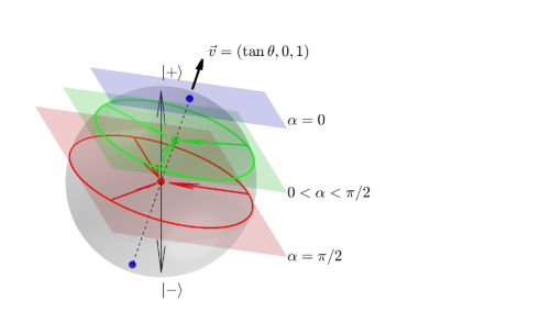
Figure 2: (Color online). Level plots of the entanglement temperature on the Bloch sphere, for an initially distributed Gaussian walker, in the limit $\xi\gg 1$. The initial coin states on the equator (red circumference, $\alpha=\pi/2$) thermalize at $T=\infty$ (red point at the center of the Bloch sphere), those in the intermediate latitude green circumference ($0<\alpha<\pi/2$)) converge to the green state at its center at some finite temperature, while the blue states at the poles, corresponding to $\alpha=1$ remainat $T=0$ during the evolution.

Equation (57) is a particular case of the general situation described in Eq.(34), since it represents a family of planes, orthogonal to the direction $({\rm{Re}}(\kappa),-{\rm{Im}}(\kappa),1)$ (see Fig.2), determined by the parameter $\kappa=\tan\theta$. This implies that initial qubit states located on the intersection of a particular plane with the Bloch sphere evolve to the same asymptotic mixed state. In particular, the extreme cases $|{\cos\alpha}|=1$ (corresponding to the initial states associated to the points $(\gamma=\theta,\varphi=0)$ and $(\gamma=\pi-\theta,\varphi=\pi)$ (the poles defined by the privileged direction) thermalize at $T_{ent}=0$. It is easy to see that these particular states are eigenstates of the coin operator $U_{\theta}$, and, accordingly, entanglement never occurs, so they remain pure during the evolution, and the global state is separable for all times $t$. This emphasizes the interpretation of the entanglement temperature as a measure of the entanglement produced between the system and its environment.

A further verification of the previous section results is possible analyzing the position of the thermal states on the Bloch sphere. A particular Bloch vector $\vec{B}$ representing the coin reduced state is

$$\vec{B}=\cos\alpha_{{}_{0}}(\sin\theta,0,\cos\theta),$$ (58)

which satisfies $|\vec{B}|=|\cos\alpha_{{}_{0}}|$. A direct calculation shows that the distance from the origin to the corresponding level plot is $d(\vec{O},\pi_{\alpha_{0}})=|{\cos\alpha_{{}_{0}}}|$. Thus every thermal state is located at the center of its corresponding level plot, which implies that the set of accessible thermal states is a diameter of the Bloch sphere, as expected. These results are illustrated in Fig. 2 and Fig. 3.

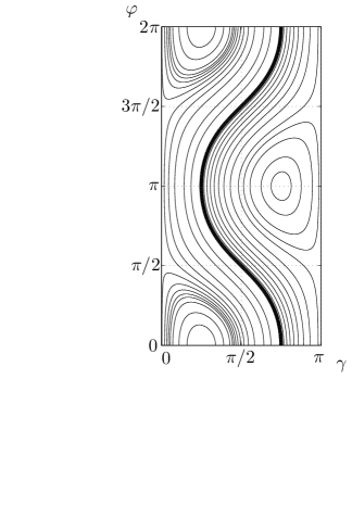
Figure 3: Level plots of the entanglement temperature in the ($\gamma,\varphi$) space, for a Hadamard walk with an initially Gaussian distributed walker. The thick central line corresponds to $T=\infty$, while the center of the closed lines are associated to the states that thermalize at $T=0$ $(\gamma=\pi/4,\varphi=0)$ and $(\gamma=3\pi/4,\varphi=\pi)$.

V Remarks and conclusions

Independence on the initial state is considered to be an important requirement for thermalization in quantum systems gogolin1 . In this work, we have shown that even in the presence of memory, there is a class of initial-state-dependent equilibrium states for which this dependence appears as a scalar factor in the exponent of a thermal state expression, allowing to identify a fixed hermitian operator that plays the role of an effective Hamiltonian, valid once the equilibrium has reached. These states are half way between being simple equilibrium states and being pure thermal states, where the dependence on the initial state disappears completely.

In the particular case of the thermal state, the effective Hamiltonian operates as a magnetic field- spin interaction. It is determined by a dimensionless parameter $\kappa$ that depends on the relevant physical parameters involved in the global dynamics, selecting a privileged direction along which the thermal states are located. In the particular case of the QW on the line, $\kappa$ is the tangent of the coin bias, $\kappa=\tan\theta$.

The initial-state-dependent entanglement temperature associated to the defined thermal states can serve as a measure of the entanglement produced between the subsystem and its environment, as illustrated in the case of a QW.

It must be emphasized the role of a large initial bath occupation for this kind of thermalization to occur. In the case of a localized walker, the system evolves to an equilibrium state that cannot be written in the exponential form with a fixed Hamiltonian, i.e., one valid for all initial states of the coin. This seems to agree with previous results, e.g. of Ref.Linden .

It is remarkable that although the example employed in this work to illustrate the theoretical results does not correspond to a typical thermal contact process, but a rather abstract one, the thermalization obtained is identical to that found in other physical systems Romanelli2 . This suggests that a more profound analysis of the underlying mathematical structure could reveal some kind of universality, aspect that needs to be explored. The study of other two-level open systems from the perspective presented in this work could be interesting, and it is currently under investigation.

References

- (1) L. S. Schulman. Phys. Rev. A 18, 2379 (1978).
- (2) J. Gemmer, M. Michel, and G. Mahler, Quantum Thermodynamics: The Emergence of Thermodynamical Behavior within Composite Quantum Systems. Lecture Notes in Physics, Springer (2004).
- (3) Juan M.R. Parrondo, Jordan M. Horowitz and Takahiro Sagawa, Nature Physics 11, 131 (2015).
- (4) John Goold, Marcus Huber, Arnau Riera, Lidia del Rio and Paul Skrzypczyk, J. Phys. A: Math. Theor 49, 143001 (2016).
- (5) Anatoli Polkivnikov and Dries Sels, Science 353, 752 (2016).
- (6) Adam M. Kaufman, M. Eric Tai, Alexander Lukin, Matthew Rispoli, Robert Schittko, Philipp M. Preiss and Markus Greiner, Science 353, 794 (2016).
- (7) A. Romanelli, Phys. Rev. A 85, 012319 (2012).
- (8) A. Romanelli, R. Donangelo, A. Vallejo, Physica A 437, 471(2015).
- (9) M. A. Novotny, F. Jin, S. Yuan, S. Miyashita, H. De Raedt, and K. Michielsen, Phys. Rev. A 93, 032110 (2016).
- (10) J. Schliemann, J. Stat. Mech. 09, P09011 (2014).
- (11) Linden, N., S. Popescu, A. Short, and A. Winter, Phys. Rev. E 79, 061103 (2009)
- (12) S. Goldstein, J. Lebowitz, R. Tumulka, and N. Zanghi, Phys.Rev.Lett. 96, 050403 (2006).
- (13) S. Popescu, A. Short, A. Winter, Nature Physics 2, 754 (2006).
- (14) M.A. Nielsen, I.L. Chuang, Quantum Computation and Quantum Information, Cambridge University Press, Cambridge (2000).
- (15) P.Bocchieri, A. Loinger, Phys. Rev. 107 (1957).
- (16) R. Kosloff, Entropy 15, 2100 (2013).
- (17) B. Travaglione, G. Milburn, Phys. Rev. A 65, 032310 (2002).
- (18) Renato Portugal, Quantum Walks and Search Algorithms. Springer, New York, (2013).
- (19) L. K. Grover. Proceedings of the 28th ACM Symposium on the Theory of Computing, 212 (1996), quant-ph/9605043 (1996).
- (20) A. Nayak, A. Vishvanath, quant-ph/0010117, (2000).
- (21) I. Carneiro, M. Loo, X. Xu, M. Girerd, V. M. Kendon, and P. L. Knight, New J. Phys. 7, 56 (2005).
- (22) G. Abal, R. Siri, A. Romanelli, and R. Donangelo, Phys. Rev. A 73, 042302, 069905(E) (2006).
- (23) M. Annabestani, M. R. Abolhasani and, G. Abal, J. Phys. A: Math. Theor. 43, 075301 (2010).
- (24) Y. Omar, N. Paunkovic, L. Sheridan, and S. Bose, Phys. Rev. A, 74, 042304 (2006)
- (25) P. K. Pathak, and G. S. Agarwal, Phys. Rev. A, 75, 032351 (2007)
- (26) C. Liu, and N. Petulante, Phys. Rev. A 79, 032312 (2009).
- (27) S. E. Venegas-Andraca, J.L. Ball, K. Burnett, and S. Bose, New J. Phys., 7, 221 (2005).
- (28) J. Endrejat, H. Büttner, J. Phys. A: Math. Gen. 38, 9289 (2005).
- (29) A.J. Bracken, D. Ellinas, and I. Tsohantjis, J. Phys. A: Math. Gen. 37, L91 (2004).
- (30) D. Ellinas, and A.J. Bracken, Phys. Rev. A 78, 052106 (2008).
- (31) O. Maloyer, and V. Kendon, New J. Phys., 9, 87 (2007).
- (32) C. Gogolin and J. Eisert, Reports on Progress in Physics 79, 056001 (2016).
- (33) A. C. Orthey, E. P. M. Amorim, Quantum Inf. Process. 16, 224 (2017).