Scaling and Balancing for High-Performance Computation of Optimal Controls

I. M. Ross
Naval Postgraduate School, Monterey, CA 93943
Q. Gong
University of California, Santa Cruz, CA 95064
M. Karpenko
Distinguished Professor and Program Director, Control and Optimization, Department of Mechanical and Aerospace Engineering.Associate Professor, Department of Applied Mathematics.Research Associate Professor and Associate Director, Control and Optimization Laboratories, Department of Mechanical and Aerospace Engineering; corresponding author: mkarpenk@nps.edu.
   R. J. Proulx
Naval Postgraduate School, Monterey, CA 93943
Research Professor, Control and Optimization Laboratories, Space Systems Academic Group.
Abstract

It is well-known that proper scaling can increase the efficiency of computational problems. In this paper we define and show that a balancing technique can substantially improve the computational efficiency of optimal control algorithms. We also show that non-canonical scaling and balancing procedures may be used quite effectively to reduce the computational difficulty of some hard problems. These results have been used successfully for several flight and field operations at NASA and DoD. A surprising aspect of our analysis shows that it may be inadvisable to use auto-scaling procedures employed in some software packages. The new results are agnostic to the specifics of the computational method; hence, they can be used to enhance the utility of any existing algorithm or software.

1 Introduction

In many practical optimal control problems, the decision variables range “wildly” in several orders of magnitude[1]. For instance, in a space trajectory optimization problem[2, 3], a position variable can vary from a few meters to well over a million kilometers. The conventional wisdom to manage the associated computational problems is to use canonical units. Many space trajectory optimizations fare well when canonical units are used[2, 3]. For instance, for low-Earth-orbiting spacecraft, one may choose the radius of the Earth (Rsubscript𝑅direct-sumR_{\oplus}) as a unit of distance, and circular speed (at Rsubscript𝑅direct-sumR_{\oplus}) as the unit of velocity. For interplanetary spacecraft, astronomical units provide a set of canonical units for scaling trajectory optimization problems. In this paper, we show that it is possible to define and use arbitrary and inconsistent units for faster trajectory optimization. For example, we may choose meters as a unit of distance along the x𝑥x-direction while concurrently using feet for distance units along the y𝑦y-direction. Furthermore, we show that it is not necessary to choose a consistent (or canonical) unit of velocity in the x𝑥x-direction to be equal to meters per second (or feet per second for velocity in the y𝑦y-direction). Thus, for example, one may “arbitrarily” choose yards per day as the unit of x𝑥x-velocity while insisting that the x𝑥x-position be measured in meters. The purpose of using such unusual or designer units[4]; i.e., highly customized units that do not necessarily conform to standardized units, is to liberate ourselves from using well-established canonical/consistent units so that we may scale an optimal control problem for faster computational results. This liberation allows us to radically alter what we mean by scaling optimal control problems, and consequently solve some apparently “hard” problems with more ease than ever before.

A second aspect of our paper is the impact of scaling on dual variables. From the Hahn-Banach theorem[5], dual variables exist for all computational optimal control problems even when they are not used. To illustrate this consequential theorem, consider the ordinary differential equation,

𝒙˙=𝒇(𝒙)˙𝒙𝒇𝒙\dot{\boldsymbol{x}}={\boldsymbol{f}}(\boldsymbol{x}) (1)

where, 𝒙Nx𝒙superscriptsubscript𝑁𝑥\boldsymbol{x}\in{\mathbb{R}}^{N_{x}} and 𝒇:𝒙Nx:𝒇maps-to𝒙superscriptsubscript𝑁𝑥{\boldsymbol{f}}:\boldsymbol{x}\mapsto{\mathbb{R}}^{N_{x}}. The formal adjoint to the variation of (1) is defined by

𝝀˙=[x𝒇]T𝝀˙𝝀superscriptdelimited-[]subscript𝑥𝒇𝑇𝝀\dot{\mbox{\boldmath$\lambda$}}=-\left[\partial_{x}{\boldsymbol{f}}\right]^{T}\,{\mbox{\boldmath$\lambda$}} (2)

where, x𝒇subscript𝑥𝒇\partial_{x}{\boldsymbol{f}} is the Jacobian of 𝒇𝒇{\boldsymbol{f}} with respect to 𝒙𝒙\boldsymbol{x}. In other words, (2) exists from the mere fact that (1) exists; hence, when a differential equation in a computational optimal control problem is scaled, it automatically affects the adjoint equation, even if it (i.e. the adjoint equation) is not used. In this paper, we show that the equations in a computational optimal control problem must be scaled in such a way that it does not “unscale” the adjoint variable even if the adjoint equation is never used in the algorithm. We call this type of scaling “balancing.”

In most algorithms – including the ones where derivatives are not used (e.g., genetic algorithms) – the “information content” in the Jacobian forms a key ingredient in the recipe that connects the sequence of iterations[6, 7, 8]. Consequently, the scales used in an optimal control problem must be balanced even if the adjoint equation is never used because it represents the information content contained in a Jacobian by way of (2). In other words, there is no escape from considering the adjoint equations. This is a fundamental result traceable to the Hahn-Banach theorem. An alternative explanation for the no-escape clause is that the adjoint equations are part of the necessary conditions for optimality. By definition, necessary conditions are indeed necessary; hence, it should not be entirely surprising that balancing is also necessary.

Our analysis also reveals another surprising result: that if scaling is performed at the discrete level, it inadvertently introduces new terms in the dynamical equations with possible feedback effects that may destabilize the search algorithm. Consequently, automatic techniques that scale the problem at the discrete level may be more harmful than useful. The simple remedy is to scale and balance the equations at the optimal-control level and choose algorithms that do not scale the equations at the discrete level. This simple “trick” has been used many number of times before by NASA[9, 10, 11, 12, 13, 14, 15, 16] and DoD[17, 18, 19, 20, 21, 22] to solve and implement on-orbit and fielded solutions. Note, however, that scaling and balancing were not at the forefront in many of these applications because their main contributions far outweighed such discussions. For instance, the focal point of [9] was the flight implementation of the optimal propellant maneuver onboard the International Space Station rather than the employment of scaling and balancing techniques. Similarly, [11] and [12] were focused on the first flight implementations of a historic zero-propellant maneuver while [15] was on the feasibility of arcsecond slews for precision pointing of the Kepler spacecraft. In the same spirit, the main contribution of [18] was the flight implementation of a shortest-time maneuver, and not on the specifics or the importance of scaling and balancing that were necessary to accomplish the on-orbit demonstration.

In this paper, we generalize the application-specific procedures of the past successes by laying down the mathematical foundations for scaling and balancing of generic optimal control algorithms. In doing so, we also demonstrate the fallacies of some scaling techniques that are currently in practice.


The journal version of this paper contains some typographical errors. Regardless, please cite the journal paper (J. Guid., Contr. & Dyn., 41/10, 2018, pp. 2086–2097) if you need to cite the results contained herein.

2 General Problem Formulation

A generic optimal control problem can be formulated as follows:

𝕏=Nx𝕌=Nu𝒙=(x1,,xNx)𝒖=(u1,,uNu)}preamble\displaystyle\left.\begin{aligned} \phantom{preamble}\mathbb{X}&={\mathbb{R}}^{N_{x}}&\mathbb{U}&={\mathbb{R}}^{N_{u}}&\\ \boldsymbol{x}&=(x_{1},\ldots,x_{N_{x}})\quad&{\boldsymbol{u}}&=(u_{1},\ldots,u_{N_{u}})&\\ \end{aligned}\hskip 81.09052pt\right\}\ \text{\emph{{preamble}}}
(B)problem{Minimize J[𝒙(),𝒖(),t0,tf]:=E(𝒙0,𝒙f,t0,tf)+t0tfF(𝒙(t),𝒖(t),t)𝑑t}costSubject to𝒙˙=𝒇(𝒙(t),𝒖(t),t)}dynamics𝒆L𝒆(𝒙0,𝒙f,t0,tf)𝒆U}events𝒉L𝒉(𝒙(t),𝒖(t),t)𝒉U}path\displaystyle\begin{aligned} \overbrace{(B)}^{\text{\normalsize\emph{{problem}}}}\left\{\begin{array}[]{ll}\text{Minimize }&\\[-12.50002pt] &\left.\begin{aligned} \makebox[76.3136pt][r]{$\displaystyle J[\boldsymbol{x}(\cdot),{\boldsymbol{u}}(\cdot),t_{0},t_{f}]:=$}&\\ \makebox[76.3136pt][r]{$\displaystyle E(\boldsymbol{x}_{0},\boldsymbol{x}_{f},t_{0},t_{f})$}&+\makebox[83.50421pt][l]{$\displaystyle\int_{t_{0}}^{t_{f}}F(\boldsymbol{x}(t),{\boldsymbol{u}}(t),t)\ dt$}\\ \end{aligned}\right\}\ \text{{\emph{cost}}}\\[20.00003pt] \text{Subject to}&\\[-15.00002pt] &\left.\begin{aligned} \makebox[76.3136pt][r]{$\displaystyle\dot{\boldsymbol{x}}$}&=\makebox[83.50421pt][l]{$\displaystyle{\boldsymbol{f}}(\boldsymbol{x}(t),{\boldsymbol{u}}(t),t)$}\\ \end{aligned}\right\}\ \text{\emph{{dynamics}}}\\[10.00002pt] &\left.\begin{aligned} \makebox[76.3136pt][r]{$\displaystyle{\boldsymbol{e}}^{L}$}&\leq\makebox[83.50421pt][l]{$\displaystyle{\boldsymbol{e}}(\boldsymbol{x}_{0},\boldsymbol{x}_{f},t_{0},t_{f})\leq{\boldsymbol{e}}^{U}$}\\ \end{aligned}\right\}\ \text{\emph{{events}}}\\[10.00002pt] &\left.\begin{aligned} \makebox[76.3136pt][r]{$\displaystyle{\boldsymbol{h}}^{L}$}&\leq\makebox[83.50421pt][l]{$\displaystyle{\boldsymbol{h}}(\boldsymbol{x}(t),{\boldsymbol{u}}(t),t)\leq{\boldsymbol{h}}^{U}$}\\ \end{aligned}\right\}\ \text{\emph{{path}}}\end{array}\right.\end{aligned}

Although the symbols used in Problem B𝐵B are fairly standard (see, for example [4]), we note the following for the purposes of completeness:

  • 𝕏𝕏\mathbb{X} and 𝕌𝕌\mathbb{U} are Nxsubscript𝑁𝑥N_{x}- and Nusubscript𝑁𝑢N_{u}-dimensional real-valued state and control spaces respectively. We assume Nx+subscript𝑁𝑥superscriptN_{x}\in\mathbb{N}^{+} and Nu+subscript𝑁𝑢superscriptN_{u}\in\mathbb{N}^{+}.

  • J𝐽J is the scalar cost function. The arguments of J𝐽J are the optimization variables.

  • The optimization variables are:

    • 𝒙()𝒙{\boldsymbol{x}(\cdot)}: the Nxsubscript𝑁𝑥N_{x}-dimensional state trajectory,

    • 𝒖()𝒖{{\boldsymbol{u}}(\cdot)}: the Nusubscript𝑁𝑢N_{u}-dimensional control trajectory,

    • t0subscript𝑡0t_{0}: the initial clock time, and

    • tfsubscript𝑡𝑓t_{f}: the final clock time.

  • E𝐸E is the scalar endpoint cost function. The arguments of E𝐸E are the endpoints. In the classical literature, E𝐸E is known as the “Mayer” cost function.

  • The endpoints are the initial state 𝒙0𝒙(t0)subscript𝒙0𝒙subscript𝑡0\boldsymbol{x}_{0}\equiv\boldsymbol{x}(t_{0}), the final state 𝒙f𝒙(tf)subscript𝒙𝑓𝒙subscript𝑡𝑓\boldsymbol{x}_{f}\equiv\boldsymbol{x}(t_{f}), the initial time t0subscript𝑡0t_{0} and the final time tfsubscript𝑡𝑓t_{f}.

  • F𝐹F is the scalar running cost function. The arguments of F𝐹F are the instantaneous value of the state variable 𝒙(t)𝒙𝑡\boldsymbol{x}(t), the instantaneous value of the control variable 𝒖(t)𝒖𝑡{\boldsymbol{u}}(t) and time t𝑡t.

  • 𝒇𝒇{\boldsymbol{f}} is the Nxsubscript𝑁𝑥N_{x}-dimensional “dynamics function,” or more appropriately the right-hand-side of the dynamics equation. The arguments of 𝒇𝒇{\boldsymbol{f}} are exactly the same as the arguments of F𝐹F.

  • 𝒆𝒆{\boldsymbol{e}} is the Nesubscript𝑁𝑒N_{e}-dimensional endpoint constraint function. The arguments of 𝒆𝒆{\boldsymbol{e}} are exactly the same as that of E𝐸E.

  • 𝒆Lsuperscript𝒆𝐿{\boldsymbol{e}}^{L} and 𝒆Usuperscript𝒆𝑈{\boldsymbol{e}}^{U} are the Nesubscript𝑁𝑒N_{e}-dimensional lower and upper bounds on the values of 𝒆𝒆{\boldsymbol{e}}.

  • 𝒉𝒉{\boldsymbol{h}} is the Nhsubscript𝑁N_{h}-dimensional path constraint function. The arguments of 𝒉𝒉{\boldsymbol{h}} are exactly the same as that of F𝐹F.

  • 𝒉Lsuperscript𝒉𝐿{\boldsymbol{h}}^{L} and 𝒉Usuperscript𝒉𝑈{\boldsymbol{h}}^{U} are the Nhsubscript𝑁N_{h}-dimensional lower and upper bounds on the values of 𝒉𝒉{\boldsymbol{h}}.

The five functions, E𝐸E, F𝐹F, 𝒇𝒇{\boldsymbol{f}}, 𝒆𝒆{\boldsymbol{e}} and 𝒉𝒉{\boldsymbol{h}} are collectively known as the data functions (for Problem B𝐵B).

Regardless of any type of method used to solve Problem B𝐵B – including the so-called direct methods – a solution to the problem must at least satisfy the necessary conditions of optimality because they are indeed necessary. The necessary conditions for Problem B𝐵B are generated by an application of Pontryagin’s Principle[4, 23, 24]. This results in the following boundary value problem (BVP), which we denote as Problem Bλsuperscript𝐵𝜆B^{\lambda}:

(Bλ){𝒙˙(t)λH¯(𝝁(t),𝝀(t),𝒙(t),𝒖(t),t)=𝟎(state eqns)𝝀˙(t)+xH¯(𝝁(t),𝝀(t),𝒙(t),𝒖(t),t)=𝟎(costate eqns)𝒉L𝒉(𝒙(t),𝒖(t),t)𝒉U(path constraint)uH¯(𝝁(t),𝝀(t),𝒙(t),𝒖(t),t)=𝟎(Hamiltonian𝝁𝒉 Minimization)𝒆L𝒆(𝒙0,𝒙f,t0,tf)𝒆U(endpoint eqns)𝝀(t0)+x0E¯(𝝂,𝒙0,𝒙f,t0,tf)=𝟎(initial and 𝝀(tf)xfE¯(𝝂,𝒙0,𝒙f,t0,tf)=𝟎final transversality𝝂𝒆conditions)[@t0]t0E¯(𝝂,𝒙0,𝒙f,t0,tf)=0(Hamiltonian[@tf]+tfE¯(𝝂,𝒙0,𝒙f,t0,tf)=0value conditons)superscript𝐵𝜆casesmissing-subexpression˙𝒙𝑡subscript𝜆¯𝐻𝝁𝑡𝝀𝑡𝒙𝑡𝒖𝑡𝑡absent0(state eqns)missing-subexpression˙𝝀𝑡subscript𝑥¯𝐻𝝁𝑡𝝀𝑡𝒙𝑡𝒖𝑡𝑡absent0(costate eqns)missing-subexpressionsuperscript𝒉𝐿𝒉𝒙𝑡𝒖𝑡𝑡absentsuperscript𝒉𝑈(path constraint)missing-subexpressionsubscript𝑢¯𝐻𝝁𝑡𝝀𝑡𝒙𝑡𝒖𝑡𝑡absent0(Hamiltonianmissing-subexpression𝝁absent𝒉 Minimization)missing-subexpressionsuperscript𝒆𝐿𝒆subscript𝒙0subscript𝒙𝑓subscript𝑡0subscript𝑡𝑓absentsuperscript𝒆𝑈(endpoint eqns)missing-subexpression𝝀subscript𝑡0subscriptsubscript𝑥0¯𝐸𝝂subscript𝒙0subscript𝒙𝑓subscript𝑡0subscript𝑡𝑓absent0(initial and missing-subexpression𝝀subscript𝑡𝑓subscriptsubscript𝑥𝑓¯𝐸𝝂subscript𝒙0subscript𝒙𝑓subscript𝑡0subscript𝑡𝑓absent0final transversalitymissing-subexpression𝝂absent𝒆conditions)missing-subexpressiondelimited-[]@subscript𝑡0subscriptsubscript𝑡0¯𝐸𝝂subscript𝒙0subscript𝒙𝑓subscript𝑡0subscript𝑡𝑓absent0(Hamiltonianmissing-subexpressiondelimited-[]@subscript𝑡𝑓subscriptsubscript𝑡𝑓¯𝐸𝝂subscript𝒙0subscript𝒙𝑓subscript𝑡0subscript𝑡𝑓absent0value conditons)\displaystyle(\textsf{$B^{\lambda}$})\left\{\begin{array}[]{lrll}&\dot{\boldsymbol{x}}(t)-\partial_{\lambda}\overline{H}({\mbox{\boldmath$\mu$}}(t),{\mbox{\boldmath$\lambda$}}(t),\boldsymbol{x}(t),{\boldsymbol{u}}(t),t)=&{\bf 0}&\text{{\emph{(state eqns)}}}\\[5.0pt] &\dot{{\mbox{\boldmath$\lambda$}}}(t)+\partial_{x}\overline{H}({\mbox{\boldmath$\mu$}}(t),{\mbox{\boldmath$\lambda$}}(t),\boldsymbol{x}(t),{\boldsymbol{u}}(t),t)=&{\bf 0}&\text{\emph{{(costate eqns)}}}\\[5.0pt] &{\boldsymbol{h}}^{L}\leq{\boldsymbol{h}}(\boldsymbol{x}(t),{\boldsymbol{u}}(t),t)\leq&{\boldsymbol{h}}^{U}&\text{\emph{{(path constraint)}}}\\[7.5pt] &\partial_{u}\overline{H}({\mbox{\boldmath$\mu$}}(t),{\mbox{\boldmath$\lambda$}}(t),\boldsymbol{x}(t),{\boldsymbol{u}}(t),t)=&{\bf 0}&\text{{\emph{(Hamiltonian}}}\\ &{\mbox{\boldmath$\mu$}}&\!\!\!\dagger\ {\boldsymbol{h}}&\text{\quad\emph{{Minimization)}}}\\[7.5pt] &{\boldsymbol{e}}^{L}\leq{\boldsymbol{e}}\big{(}\boldsymbol{x}_{0},\boldsymbol{x}_{f},t_{0},t_{f}\big{)}\leq&{\boldsymbol{e}}^{U}&\text{\emph{{(endpoint eqns)}}}\\[7.5pt] &{\mbox{\boldmath$\lambda$}}(t_{0})+\partial_{x_{0}}\overline{E}({\mbox{\boldmath$\nu$}},\boldsymbol{x}_{0},\boldsymbol{x}_{f},t_{0},t_{f})=&{\bf 0}&\text{\emph{{(initial and}} }\\ &{\mbox{\boldmath$\lambda$}}(t_{f})-\partial_{x_{f}}\overline{E}({\mbox{\boldmath$\nu$}},\boldsymbol{x}_{0},\boldsymbol{x}_{f},t_{0},t_{f})=&{\bf 0}&\text{\emph{{final transversality}}}\\ &{\mbox{\boldmath$\nu$}}&\!\!\!\dagger\ {\boldsymbol{e}}&\text{{\emph{conditions)}}}\\[7.5pt] &\mathcal{H}[@t_{0}]-\partial_{t_{0}}\overline{E}({\mbox{\boldmath$\nu$}},\boldsymbol{x}_{0},\boldsymbol{x}_{f},t_{0},t_{f})=&0&\text{{\emph{(Hamiltonian}}}\\ &\mathcal{H}[@t_{f}]+\partial_{t_{f}}\overline{E}({\mbox{\boldmath$\nu$}},\boldsymbol{x}_{0},\boldsymbol{x}_{f},t_{0},t_{f})=&0&\text{\emph{{value conditons)}}}\\ \end{array}\right.

In Problem Bλsuperscript𝐵𝜆B^{\lambda}, the unknowns are:

  1. 1.

    The system trajectory, t(𝒙,𝒖)Nx×Numaps-to𝑡𝒙𝒖superscriptsubscript𝑁𝑥superscriptsubscript𝑁𝑢t\mapsto(\boldsymbol{x},{\boldsymbol{u}})\in{\mathbb{R}}^{N_{x}}\times{\mathbb{R}}^{N_{u}};

  2. 2.

    The adjoint covector function, t𝝀Nxmaps-to𝑡𝝀superscriptsubscript𝑁𝑥t\mapsto{\mbox{\boldmath$\lambda$}}\in{\mathbb{R}}^{N_{x}};

  3. 3.

    The path covector function, t𝝁Nhmaps-to𝑡𝝁superscriptsubscript𝑁t\mapsto{\mbox{\boldmath$\mu$}}\in{\mathbb{R}}^{N_{h}};

  4. 4.

    The endpoint covector, 𝝂Ne𝝂superscriptsubscript𝑁𝑒{\mbox{\boldmath$\nu$}}\in{\mathbb{R}}^{N_{e}}; and

  5. 5.

    The initial and final clock times, t0subscript𝑡0t_{0}\in\mathbb{R} and tfsubscript𝑡𝑓t_{f}\in\mathbb{R}.

The quantity H¯¯𝐻\overline{H} is the Lagrangian of the Hamiltonian given by

H¯(𝝁,𝝀,𝒙,𝒖,t):=H(𝝀,𝒙,𝒖,t)+𝝁T𝒉(𝒙,𝒖,t)assign¯𝐻𝝁𝝀𝒙𝒖𝑡𝐻𝝀𝒙𝒖𝑡superscript𝝁𝑇𝒉𝒙𝒖𝑡\overline{H}({\mbox{\boldmath$\mu$}},{\mbox{\boldmath$\lambda$}},\boldsymbol{x},{\boldsymbol{u}},t):=H({\mbox{\boldmath$\lambda$}},\boldsymbol{x},{\boldsymbol{u}},t)+{\mbox{\boldmath$\mu$}}^{T}{\boldsymbol{h}}(\boldsymbol{x},{\boldsymbol{u}},t)

where H𝐻H is the usual Pontryagin Hamiltonian,

H(𝝀,𝒙,𝒖,t):=F(𝒙,𝒖,t)+𝝀T𝒇(𝒙,𝒖,t)assign𝐻𝝀𝒙𝒖𝑡𝐹𝒙𝒖𝑡superscript𝝀𝑇𝒇𝒙𝒖𝑡H({\mbox{\boldmath$\lambda$}},\boldsymbol{x},{\boldsymbol{u}},t):=F(\boldsymbol{x},{\boldsymbol{u}},t)+{\mbox{\boldmath$\lambda$}}^{T}{\boldsymbol{f}}(\boldsymbol{x},{\boldsymbol{u}},t)

and \mathcal{H} is the lower or minimized Hamiltonian,

(𝝀,𝒙,t):=min𝒖H(𝝀,𝒙,𝒖,t)assign𝝀𝒙𝑡subscript𝒖𝐻𝝀𝒙𝒖𝑡\mathcal{H}({\mbox{\boldmath$\lambda$}},\boldsymbol{x},t):=\min_{{\boldsymbol{u}}}H({\mbox{\boldmath$\lambda$}},\boldsymbol{x},{\boldsymbol{u}},t)

The symbol [@t]delimited-[]@𝑡\mathcal{H}[@t] is a shorthand for (𝝀(t),𝒙(t),t)𝝀𝑡𝒙𝑡𝑡\mathcal{H}({\mbox{\boldmath$\lambda$}}(t),\boldsymbol{x}(t),t). The quantity E¯¯𝐸{\overline{E}} is the Endpoint Lagrangian given by,

E¯(𝝂,𝒙0,𝒙f,t0,tf):=E(𝒙0,𝒙f,t0,tf)+𝝂T𝒆(𝒙0,𝒙f,t0,tf)assign¯𝐸𝝂subscript𝒙0subscript𝒙𝑓subscript𝑡0subscript𝑡𝑓𝐸subscript𝒙0subscript𝒙𝑓subscript𝑡0subscript𝑡𝑓superscript𝝂𝑇𝒆subscript𝒙0subscript𝒙𝑓subscript𝑡0subscript𝑡𝑓{\overline{E}}({\mbox{\boldmath$\nu$}},\boldsymbol{x}_{0},\boldsymbol{x}_{f},t_{0},t_{f}):=E(\boldsymbol{x}_{0},\boldsymbol{x}_{f},t_{0},t_{f})+{\mbox{\boldmath$\nu$}}^{T}{\boldsymbol{e}}(\boldsymbol{x}_{0},\boldsymbol{x}_{f},t_{0},t_{f})

The \dagger notation used in defining Problem Bλsuperscript𝐵𝜆B^{\lambda} denotes complementarity conditions[4]. For instance, 𝝂𝒆𝝂𝒆{\mbox{\boldmath$\nu$}}\,\dagger\,{\boldsymbol{e}} is a shorthand for the conditions

νi{0ifei(𝒙0,𝒙f,t0,tf)=eiL=0ifeiL<ei(𝒙0,𝒙f,t0,tf)<eiU0ifei(𝒙0,𝒙f,t0,tf)=eiUunrestrictedifeiL=eiUsubscript𝜈𝑖casesabsent0𝑖𝑓subscript𝑒𝑖subscript𝒙0subscript𝒙𝑓subscript𝑡0subscript𝑡𝑓absentsuperscriptsubscript𝑒𝑖𝐿absent0𝑖𝑓superscriptsubscript𝑒𝑖𝐿subscript𝑒𝑖subscript𝒙0subscript𝒙𝑓subscript𝑡0subscript𝑡𝑓absentsuperscriptsubscript𝑒𝑖𝑈absent0𝑖𝑓subscript𝑒𝑖subscript𝒙0subscript𝒙𝑓subscript𝑡0subscript𝑡𝑓absentsuperscriptsubscript𝑒𝑖𝑈𝑢𝑛𝑟𝑒𝑠𝑡𝑟𝑖𝑐𝑡𝑒𝑑𝑖𝑓superscriptsubscript𝑒𝑖𝐿absentsuperscriptsubscript𝑒𝑖𝑈\nu_{i}\left\{\begin{array}[]{ccrc}\leq 0&if&e_{i}(\boldsymbol{x}_{0},\boldsymbol{x}_{f},t_{0},t_{f})&=e_{i}^{L}\\ =0&if&\qquad e_{i}^{L}<e_{i}(\boldsymbol{x}_{0},\boldsymbol{x}_{f},t_{0},t_{f})&<e_{i}^{U}\\ \geq 0&if&e_{i}(\boldsymbol{x}_{0},\boldsymbol{x}_{f},t_{0},t_{f})&=e_{i}^{U}\\ unrestricted&if&e_{i}^{L}&=e_{i}^{U}\end{array}\right. (4)

with 𝝁𝒉𝝁𝒉{\mbox{\boldmath$\mu$}}\,\dagger\,{\boldsymbol{h}} defined similarly (for each t𝑡t).

3 Scaling the Primal Problem

We change the coordinates of the unknown variables of Problem B𝐵B according to the affine transformations,

𝒙:=assign𝒙absent\displaystyle\boldsymbol{x}:= 𝑷x𝒙~+𝒒xsubscript𝑷𝑥~𝒙subscript𝒒𝑥\displaystyle{\boldsymbol{P}}_{x}\ {\widetilde{\boldsymbol{x}}}+{\boldsymbol{q}}_{x} (5a)
𝒖:=assign𝒖absent\displaystyle{\boldsymbol{u}}:= 𝑷u𝒖~+𝒒usubscript𝑷𝑢~𝒖subscript𝒒𝑢\displaystyle{\boldsymbol{P}}_{u}\ {\widetilde{{\boldsymbol{u}}}}+{\boldsymbol{q}}_{u} (5b)
t:=assign𝑡absent\displaystyle t:= ptt~+qtsubscript𝑝𝑡~𝑡subscript𝑞𝑡\displaystyle p_{t}\ \widetilde{t}+q_{t} (5c)

where, the uppercase letter 𝑷()subscript𝑷{\boldsymbol{P}}_{(\cdot)} denotes an invertible square matrix of appropriate dimensions, and the lower case letter p()subscript𝑝p_{(\cdot)} is a scalar. Similarly 𝒒()subscript𝒒{\boldsymbol{q}}_{(\cdot)} is a vector of appropriate dimension and q()subscript𝑞q_{(\cdot)} is a scalar. The tilde (similar-to\sim) variables are the transformed variables. In similar fashion, we “scale” the cost functional J𝐽J, the endpoint constraint function 𝒆𝒆{\boldsymbol{e}} and the path constraint function 𝒉𝒉{\boldsymbol{h}} according to,

J:=assign𝐽absent\displaystyle J:= pJJ~+qJsubscript𝑝𝐽~𝐽subscript𝑞𝐽\displaystyle p_{J}\ \widetilde{J}+q_{J} (6a)
𝒆:=assign𝒆absent\displaystyle{\boldsymbol{e}}:= 𝑷e𝒆~+𝒒esubscript𝑷𝑒~𝒆subscript𝒒𝑒\displaystyle{\boldsymbol{P}}_{e}\ {\widetilde{{\boldsymbol{e}}}}+{\boldsymbol{q}}_{e} (6b)
𝒉:=assign𝒉absent\displaystyle{\boldsymbol{h}}:= 𝑷h𝒉~+𝒒hsubscript𝑷~𝒉subscript𝒒\displaystyle{\boldsymbol{P}}_{h}\ {\widetilde{{\boldsymbol{h}}}}+{\boldsymbol{q}}_{h} (6c)

where, pJ>0subscript𝑝𝐽0p_{J}>0, and 𝑷esubscript𝑷𝑒{\boldsymbol{P}}_{e} and 𝑷hsubscript𝑷{\boldsymbol{P}}_{h} are positive definite diagonal matrices. Let Problem B~~𝐵\widetilde{B} denote the transformation of Problem B𝐵B resulting from (5) and (6). This problem can be explicitly obtained as follows: First, the transformation of J𝐽J to J~~𝐽\widetilde{J} can be constructed using (5) as,

J[𝒙(),𝒖(),t0,tf]𝐽𝒙𝒖subscript𝑡0subscript𝑡𝑓\displaystyle J[{\boldsymbol{x}(\cdot)},{{\boldsymbol{u}}(\cdot)},t_{0},t_{f}] =J[𝑷x𝒙~()+𝒒x,𝑷u𝒖~()+𝒒u,ptt~0+qt,ptt~f+qt]absent𝐽subscript𝑷𝑥~𝒙subscript𝒒𝑥subscript𝑷𝑢~𝒖subscript𝒒𝑢subscript𝑝𝑡subscript~𝑡0subscript𝑞𝑡subscript𝑝𝑡subscript~𝑡𝑓subscript𝑞𝑡\displaystyle=J[{\boldsymbol{P}}_{x}{\widetilde{\boldsymbol{x}}}(\cdot)+{\boldsymbol{q}}_{x},\ {\boldsymbol{P}}_{u}{\widetilde{{\boldsymbol{u}}}}(\cdot)+{\boldsymbol{q}}_{u},\ p_{t}\widetilde{t}_{0}+q_{t},\ p_{t}\widetilde{t}_{f}+q_{t}]
:=pJJ~[𝒙~(),𝒖~(),t~0,t~f]+qJassignabsentsubscript𝑝𝐽~𝐽~𝒙~𝒖subscript~𝑡0subscript~𝑡𝑓subscript𝑞𝐽\displaystyle:=p_{J}\widetilde{J}[{\widetilde{\boldsymbol{x}}}(\cdot),{\widetilde{{\boldsymbol{u}}}}(\cdot),\widetilde{t}_{0},\widetilde{t}_{f}]+q_{J} (7)

where the last equality in (7) follows from (6). Hence, the cost functional transforms according to,

J~[𝒙~(),𝒖~(),t~0,t~f]:=assign~𝐽~𝒙~𝒖subscript~𝑡0subscript~𝑡𝑓absent\displaystyle\widetilde{J}[{\widetilde{\boldsymbol{x}}}(\cdot),{\widetilde{{\boldsymbol{u}}}}(\cdot),\widetilde{t}_{0},\widetilde{t}_{f}]:= qJpJ+1pJJ[𝑷x𝒙~()+𝒒x,𝑷u𝒖~()+𝒒u,ptt~0+qt,ptt~f+qt]subscript𝑞𝐽subscript𝑝𝐽1subscript𝑝𝐽𝐽subscript𝑷𝑥~𝒙subscript𝒒𝑥subscript𝑷𝑢~𝒖subscript𝒒𝑢subscript𝑝𝑡subscript~𝑡0subscript𝑞𝑡subscript𝑝𝑡subscript~𝑡𝑓subscript𝑞𝑡\displaystyle-\frac{q_{J}}{p_{J}}+\frac{1}{p_{J}}J[{\boldsymbol{P}}_{x}{\widetilde{\boldsymbol{x}}}(\cdot)+{\boldsymbol{q}}_{x},\ {\boldsymbol{P}}_{u}{\widetilde{{\boldsymbol{u}}}}(\cdot)+{\boldsymbol{q}}_{u},\ p_{t}\widetilde{t}_{0}+q_{t},\ p_{t}\widetilde{t}_{f}+q_{t}]
=\displaystyle= qJpJ+1pJE(𝑷x𝒙~0+𝒒x,𝑷x𝒙~f+𝒒x,ptt~0+qt,ptt~f+qt)subscript𝑞𝐽subscript𝑝𝐽1subscript𝑝𝐽𝐸subscript𝑷𝑥subscript~𝒙0subscript𝒒𝑥subscript𝑷𝑥subscript~𝒙𝑓subscript𝒒𝑥subscript𝑝𝑡subscript~𝑡0subscript𝑞𝑡subscript𝑝𝑡subscript~𝑡𝑓subscript𝑞𝑡\displaystyle-\frac{q_{J}}{p_{J}}+\frac{1}{p_{J}}E({\boldsymbol{P}}_{x}{\widetilde{\boldsymbol{x}}}_{0}+{\boldsymbol{q}}_{x},\ {\boldsymbol{P}}_{x}{\widetilde{\boldsymbol{x}}}_{f}+{\boldsymbol{q}}_{x},\ p_{t}\widetilde{t}_{0}+q_{t},\ p_{t}\widetilde{t}_{f}+q_{t})
+ptpJt~0t~fF(𝑷x𝒙~(t)+𝒒x,𝑷u𝒖~(t)+𝒒u,ptt~+qt)𝑑t~subscript𝑝𝑡subscript𝑝𝐽superscriptsubscriptsubscript~𝑡0subscript~𝑡𝑓𝐹subscript𝑷𝑥~𝒙𝑡subscript𝒒𝑥subscript𝑷𝑢~𝒖𝑡subscript𝒒𝑢subscript𝑝𝑡~𝑡subscript𝑞𝑡differential-d~𝑡\displaystyle+\frac{p_{t}}{p_{J}}\int_{\widetilde{t}_{0}}^{\widetilde{t}_{f}}F({\boldsymbol{P}}_{x}{\widetilde{\boldsymbol{x}}}(t)+{\boldsymbol{q}}_{x},\ {\boldsymbol{P}}_{u}{\widetilde{{\boldsymbol{u}}}}(t)+{\boldsymbol{q}}_{u},\ p_{t}\widetilde{t}+q_{t})\ d\widetilde{t} (8)

where t𝑡t in the integrand in (8) is to be understood as (ptt~+qt)subscript𝑝𝑡~𝑡subscript𝑞𝑡(p_{t}\widetilde{t}+q_{t}).

The transformation of the dynamics is given by,

d𝒙dt=𝑷xptd𝒙~dt~=𝒇(𝑷x𝒙~(t)+𝒒x,𝑷u𝒖~(t)+𝒒u,ptt~+qt)𝑑𝒙𝑑𝑡subscript𝑷𝑥subscript𝑝𝑡𝑑~𝒙𝑑~𝑡𝒇subscript𝑷𝑥~𝒙𝑡subscript𝒒𝑥subscript𝑷𝑢~𝒖𝑡subscript𝒒𝑢subscript𝑝𝑡~𝑡subscript𝑞𝑡\displaystyle\frac{d\boldsymbol{x}}{dt}=\frac{{\boldsymbol{P}}_{x}}{p_{t}}\frac{d{\widetilde{\boldsymbol{x}}}}{d\widetilde{t}}={\boldsymbol{f}}({\boldsymbol{P}}_{x}{\widetilde{\boldsymbol{x}}}(t)+{\boldsymbol{q}}_{x},\ {\boldsymbol{P}}_{u}{\widetilde{{\boldsymbol{u}}}}(t)+{\boldsymbol{q}}_{u},\ p_{t}\widetilde{t}+q_{t})

Hence, the dynamical equations transform according to,

d𝒙~dt~=𝒇~(𝒙~(t),𝒖~(t),t~):=pt𝑷x1𝒇(𝑷x𝒙~(t)+𝒒x,𝑷u𝒖~(t)+𝒒u,ptt~+qt)𝑑~𝒙𝑑~𝑡~𝒇~𝒙𝑡~𝒖𝑡~𝑡assignsubscript𝑝𝑡subscriptsuperscript𝑷1𝑥𝒇subscript𝑷𝑥~𝒙𝑡subscript𝒒𝑥subscript𝑷𝑢~𝒖𝑡subscript𝒒𝑢subscript𝑝𝑡~𝑡subscript𝑞𝑡\displaystyle\frac{d{\widetilde{\boldsymbol{x}}}}{d\widetilde{t}}=\widetilde{{\boldsymbol{f}}}({\widetilde{\boldsymbol{x}}}(t),{\widetilde{{\boldsymbol{u}}}}(t),\widetilde{t}):=p_{t}{\boldsymbol{P}}^{-1}_{x}{\boldsymbol{f}}({\boldsymbol{P}}_{x}{\widetilde{\boldsymbol{x}}}(t)+{\boldsymbol{q}}_{x},\ {\boldsymbol{P}}_{u}{\widetilde{{\boldsymbol{u}}}}(t)+{\boldsymbol{q}}_{u},\ p_{t}\widetilde{t}+q_{t}) (9)

where, we have once again used t𝑡t in (9) to mean (ptt~+qt)subscript𝑝𝑡~𝑡subscript𝑞𝑡(p_{t}\widetilde{t}+q_{t}).

By using similar procedures, it follows that the endpoint and path constraint functions transform according to,

𝒆~(𝒙~0,𝒙~f,t~0,t~f)=~𝒆subscript~𝒙0subscript~𝒙𝑓subscript~𝑡0subscript~𝑡𝑓absent\displaystyle{\widetilde{{\boldsymbol{e}}}}\big{(}{\widetilde{\boldsymbol{x}}}_{0},{\widetilde{\boldsymbol{x}}}_{f},\widetilde{t}_{0},\widetilde{t}_{f}\big{)}= 𝑷e1[𝒆(𝑷x𝒙~0+𝒒x,𝑷x𝒙~f+𝒒x,ptt~0+qt,ptt~f+qt)𝒒e]superscriptsubscript𝑷𝑒1delimited-[]𝒆subscript𝑷𝑥subscript~𝒙0subscript𝒒𝑥subscript𝑷𝑥subscript~𝒙𝑓subscript𝒒𝑥subscript𝑝𝑡subscript~𝑡0subscript𝑞𝑡subscript𝑝𝑡subscript~𝑡𝑓subscript𝑞𝑡subscript𝒒𝑒\displaystyle{\boldsymbol{P}}_{e}^{-1}\left[{\boldsymbol{e}}\big{(}{\boldsymbol{P}}_{x}{\widetilde{\boldsymbol{x}}}_{0}+{\boldsymbol{q}}_{x},\ {\boldsymbol{P}}_{x}{\widetilde{\boldsymbol{x}}}_{f}+{\boldsymbol{q}}_{x},\ p_{t}\widetilde{t}_{0}+q_{t},\ p_{t}\widetilde{t}_{f}+q_{t}\big{)}-{\boldsymbol{q}}_{e}\right] (10)
𝒉~(𝒙~(t~),𝒖~(t~),t~)=~𝒉~𝒙~𝑡~𝒖~𝑡~𝑡absent\displaystyle{\widetilde{{\boldsymbol{h}}}}({\widetilde{\boldsymbol{x}}}(\widetilde{t}),{\widetilde{{\boldsymbol{u}}}}(\widetilde{t}),\widetilde{t})= 𝑷h1[𝒉(𝑷x𝒙~(t)+𝒒x,𝑷u𝒖~(t)+𝒒u,ptt~+qt)𝒒h]superscriptsubscript𝑷1delimited-[]𝒉subscript𝑷𝑥~𝒙𝑡subscript𝒒𝑥subscript𝑷𝑢~𝒖𝑡subscript𝒒𝑢subscript𝑝𝑡~𝑡subscript𝑞𝑡subscript𝒒\displaystyle{\boldsymbol{P}}_{h}^{-1}\big{[}{\boldsymbol{h}}\big{(}{\boldsymbol{P}}_{x}{\widetilde{\boldsymbol{x}}}(t)+{\boldsymbol{q}}_{x},\ {\boldsymbol{P}}_{u}{\widetilde{{\boldsymbol{u}}}}(t)+{\boldsymbol{q}}_{u},\ p_{t}\widetilde{t}+q_{t}\big{)}-{\boldsymbol{q}}_{h}\big{]} (11)

The corresponding lower and upper bounds are given by,

𝒆~Lsuperscript~𝒆𝐿\displaystyle\widetilde{{\boldsymbol{e}}}^{L} =𝑷e1(𝒆L𝒒e),absentsuperscriptsubscript𝑷𝑒1superscript𝒆𝐿subscript𝒒𝑒\displaystyle={\boldsymbol{P}}_{e}^{-1}({\boldsymbol{e}}^{L}-{\boldsymbol{q}}_{e}), 𝒆~Usuperscript~𝒆𝑈\displaystyle\widetilde{{\boldsymbol{e}}}^{U} =𝑷e1(𝒆U𝒒e)absentsuperscriptsubscript𝑷𝑒1superscript𝒆𝑈subscript𝒒𝑒\displaystyle={\boldsymbol{P}}_{e}^{-1}({\boldsymbol{e}}^{U}-{\boldsymbol{q}}_{e}) (12)
𝒉~Lsuperscript~𝒉𝐿\displaystyle\widetilde{{\boldsymbol{h}}}^{L} =𝑷h1(𝒉L𝒒h),absentsuperscriptsubscript𝑷1superscript𝒉𝐿subscript𝒒\displaystyle={\boldsymbol{P}}_{h}^{-1}({\boldsymbol{h}}^{L}-{\boldsymbol{q}}_{h}), 𝒉~Usuperscript~𝒉𝑈\displaystyle\widetilde{{\boldsymbol{h}}}^{U} =𝑷h1(𝒉U𝒒h)absentsuperscriptsubscript𝑷1superscript𝒉𝑈subscript𝒒\displaystyle={\boldsymbol{P}}_{h}^{-1}({\boldsymbol{h}}^{U}-{\boldsymbol{q}}_{h}) (13)

Equations (8)-(13) constitute Problem B~~𝐵\widetilde{B}.

4 Necessary Conditions for the Scaled Problem

Let 𝝀~,𝝁~~𝝀~𝝁{\widetilde{{\mbox{\boldmath$\lambda$}}}},{\widetilde{{\mbox{\boldmath$\mu$}}}} and 𝝂~~𝝂{\widetilde{{\mbox{\boldmath$\nu$}}}} be the adjoint, path and endpoint covectors respectively, associated with the necessary conditions for Problem B~~𝐵\widetilde{B}. Then, it follows that the Hamiltonian, the Lagrangian of the Hamiltonian, and the Endpoint Lagrangian for Problem B~~𝐵\widetilde{B} are given by[4]:

  • The Hamiltonian, H~~𝐻\widetilde{H}:

    H~(𝝀~,𝒙~,𝒖~,t~):=assign~𝐻~𝝀~𝒙~𝒖~𝑡absent\displaystyle\widetilde{H}({\widetilde{{\mbox{\boldmath$\lambda$}}}},{\widetilde{\boldsymbol{x}}},{\widetilde{{\boldsymbol{u}}}},\widetilde{t}):= ptpJF(𝑷x𝒙~(t)+𝒒x,𝑷u𝒖~(t)+𝒒u,ptt~+qt)subscript𝑝𝑡subscript𝑝𝐽𝐹subscript𝑷𝑥~𝒙𝑡subscript𝒒𝑥subscript𝑷𝑢~𝒖𝑡subscript𝒒𝑢subscript𝑝𝑡~𝑡subscript𝑞𝑡\displaystyle\frac{p_{t}}{p_{J}}F({\boldsymbol{P}}_{x}{\widetilde{\boldsymbol{x}}}(t)+{\boldsymbol{q}}_{x},\ {\boldsymbol{P}}_{u}{\widetilde{{\boldsymbol{u}}}}(t)+{\boldsymbol{q}}_{u},\ p_{t}\widetilde{t}+q_{t})
    +pt𝝀~T𝑷x1𝒇(𝑷x𝒙~(t)+𝒒x,𝑷u𝒖~(t)+𝒒u,ptt~+qt)subscript𝑝𝑡superscript~𝝀𝑇subscriptsuperscript𝑷1𝑥𝒇subscript𝑷𝑥~𝒙𝑡subscript𝒒𝑥subscript𝑷𝑢~𝒖𝑡subscript𝒒𝑢subscript𝑝𝑡~𝑡subscript𝑞𝑡\displaystyle\qquad+p_{t}{\widetilde{{\mbox{\boldmath$\lambda$}}}}^{T}{\boldsymbol{P}}^{-1}_{x}{\boldsymbol{f}}({\boldsymbol{P}}_{x}{\widetilde{\boldsymbol{x}}}(t)+{\boldsymbol{q}}_{x},\ {\boldsymbol{P}}_{u}{\widetilde{{\boldsymbol{u}}}}(t)+{\boldsymbol{q}}_{u},\ p_{t}\widetilde{t}+q_{t}) (14)
  • The Lagrangian of the Hamiltonian, H~¯¯~𝐻\overline{\widetilde{H}}:

    H~¯(𝝁~,𝝀~,𝒙~,𝒖~,t~)¯~𝐻~𝝁~𝝀~𝒙~𝒖~𝑡\displaystyle\overline{\widetilde{H}}({\widetilde{{\mbox{\boldmath$\mu$}}}},{\widetilde{{\mbox{\boldmath$\lambda$}}}},{\widetilde{\boldsymbol{x}}},{\widetilde{{\boldsymbol{u}}}},\widetilde{t}) :=H~(𝝀~,𝒙~,𝒖~,t~)assignabsent~𝐻~𝝀~𝒙~𝒖~𝑡\displaystyle:=\widetilde{H}({\widetilde{{\mbox{\boldmath$\lambda$}}}},{\widetilde{\boldsymbol{x}}},{\widetilde{{\boldsymbol{u}}}},\widetilde{t})
    +𝝁~T𝑷h1[𝒉(𝑷x𝒙~(t)+𝒒x,𝑷u𝒖~(t)+𝒒u,ptt~+qt)𝒒h]superscript~𝝁𝑇superscriptsubscript𝑷1delimited-[]𝒉subscript𝑷𝑥~𝒙𝑡subscript𝒒𝑥subscript𝑷𝑢~𝒖𝑡subscript𝒒𝑢subscript𝑝𝑡~𝑡subscript𝑞𝑡subscript𝒒\displaystyle\qquad+{\widetilde{{\mbox{\boldmath$\mu$}}}}^{T}{\boldsymbol{P}}_{h}^{-1}\big{[}{\boldsymbol{h}}\big{(}{\boldsymbol{P}}_{x}{\widetilde{\boldsymbol{x}}}(t)+{\boldsymbol{q}}_{x},\ {\boldsymbol{P}}_{u}{\widetilde{{\boldsymbol{u}}}}(t)+{\boldsymbol{q}}_{u},\ p_{t}\widetilde{t}+q_{t}\big{)}-{\boldsymbol{q}}_{h}\big{]} (15)
  • The Endpoint Lagrangian E~¯¯~𝐸\overline{\widetilde{E}}:

    E~¯(𝝂~,𝒙~0,𝒙~f,t~0,t~f):=1pJE(𝑷x𝒙~0+𝒒x,𝑷x𝒙~f+𝒒x,ptt~0+qt,ptt~f+qt)assign¯~𝐸~𝝂subscript~𝒙0subscript~𝒙𝑓subscript~𝑡0subscript~𝑡𝑓1subscript𝑝𝐽𝐸subscript𝑷𝑥subscript~𝒙0subscript𝒒𝑥subscript𝑷𝑥subscript~𝒙𝑓subscript𝒒𝑥subscript𝑝𝑡subscript~𝑡0subscript𝑞𝑡subscript𝑝𝑡subscript~𝑡𝑓subscript𝑞𝑡\displaystyle\overline{\widetilde{E}}({\widetilde{{\mbox{\boldmath$\nu$}}}},{\widetilde{\boldsymbol{x}}}_{0},{\widetilde{\boldsymbol{x}}}_{f},\widetilde{t}_{0},\widetilde{t}_{f}):=\frac{1}{p_{J}}E({\boldsymbol{P}}_{x}{\widetilde{\boldsymbol{x}}}_{0}+{\boldsymbol{q}}_{x},\ {\boldsymbol{P}}_{x}{\widetilde{\boldsymbol{x}}}_{f}+{\boldsymbol{q}}_{x},\ p_{t}\widetilde{t}_{0}+q_{t},\ p_{t}\widetilde{t}_{f}+q_{t})
    +𝝂~T𝑷e1[𝒆(𝑷x𝒙~0+𝒒x,𝑷x𝒙~f+𝒒x,ptt~0+qt,ptt~f+qt)𝒒e]superscript~𝝂𝑇superscriptsubscript𝑷𝑒1delimited-[]𝒆subscript𝑷𝑥subscript~𝒙0subscript𝒒𝑥subscript𝑷𝑥subscript~𝒙𝑓subscript𝒒𝑥subscript𝑝𝑡subscript~𝑡0subscript𝑞𝑡subscript𝑝𝑡subscript~𝑡𝑓subscript𝑞𝑡subscript𝒒𝑒\displaystyle\qquad+{\widetilde{{\mbox{\boldmath$\nu$}}}}^{T}{\boldsymbol{P}}_{e}^{-1}\left[{\boldsymbol{e}}\big{(}{\boldsymbol{P}}_{x}{\widetilde{\boldsymbol{x}}}_{0}+{\boldsymbol{q}}_{x},\ {\boldsymbol{P}}_{x}{\widetilde{\boldsymbol{x}}}_{f}+{\boldsymbol{q}}_{x},\ p_{t}\widetilde{t}_{0}+q_{t},\ p_{t}\widetilde{t}_{f}+q_{t}\big{)}-{\boldsymbol{q}}_{e}\right] (16)

The adjoint equation for Problem B~~𝐵\widetilde{B} is given by,

d𝝀~dt~=H~¯𝒙~𝑑~𝝀𝑑~𝑡¯~𝐻~𝒙-\frac{d{\widetilde{{\mbox{\boldmath$\lambda$}}}}}{d\widetilde{t}}=\frac{\partial\overline{\widetilde{H}}}{\partial{\widetilde{\boldsymbol{x}}}} (17)

Evaluating the right-hand-side of (17) using (15) we get,

d𝝀~dt~=ptpJ𝑷xT[F𝒙]+pt[𝑷x1𝒇𝒙𝑷x]T𝝀~+[𝑷h1𝒉𝒙𝑷x]T𝝁~𝑑~𝝀𝑑~𝑡subscript𝑝𝑡subscript𝑝𝐽superscriptsubscript𝑷𝑥𝑇delimited-[]𝐹𝒙subscript𝑝𝑡superscriptdelimited-[]superscriptsubscript𝑷𝑥1𝒇𝒙subscript𝑷𝑥𝑇~𝝀superscriptdelimited-[]superscriptsubscript𝑷1𝒉𝒙subscript𝑷𝑥𝑇~𝝁\displaystyle-\frac{d{\widetilde{{\mbox{\boldmath$\lambda$}}}}}{d\widetilde{t}}=\frac{p_{t}}{p_{J}}{\boldsymbol{P}}_{x}^{T}\left[\frac{\partial F}{\partial\boldsymbol{x}}\right]+p_{t}\left[{\boldsymbol{P}}_{x}^{-1}\frac{\partial{\boldsymbol{f}}}{\partial\boldsymbol{x}}{\boldsymbol{P}}_{x}\right]^{T}{\widetilde{{\mbox{\boldmath$\lambda$}}}}+\left[{\boldsymbol{P}}_{h}^{-1}\frac{\partial{\boldsymbol{h}}}{\partial\boldsymbol{x}}{\boldsymbol{P}}_{x}\right]^{T}{\widetilde{{\mbox{\boldmath$\mu$}}}} (18)

Following the same process for the stationarity condition associated with the Hamiltonian minimization condition for Problem B~~𝐵\widetilde{B}, we get,

H~¯𝒖~=ptpJ𝑷uT(F𝒖)+pt𝑷uT(𝒇𝒖)T(𝑷x1)T𝝀~+𝑷uT(𝒉𝒖)T(𝑷h1)T𝝁~=𝟎¯~𝐻~𝒖subscript𝑝𝑡subscript𝑝𝐽superscriptsubscript𝑷𝑢𝑇𝐹𝒖subscript𝑝𝑡superscriptsubscript𝑷𝑢𝑇superscript𝒇𝒖𝑇superscriptsuperscriptsubscript𝑷𝑥1𝑇~𝝀superscriptsubscript𝑷𝑢𝑇superscript𝒉𝒖𝑇superscriptsuperscriptsubscript𝑷1𝑇~𝝁0\frac{\partial\overline{\widetilde{H}}}{\partial{\widetilde{{\boldsymbol{u}}}}}=\frac{p_{t}}{p_{J}}{\boldsymbol{P}}_{u}^{T}\left(\frac{\partial F}{\partial{\boldsymbol{u}}}\right)+p_{t}{\boldsymbol{P}}_{u}^{T}\left(\frac{\partial{\boldsymbol{f}}}{\partial{\boldsymbol{u}}}\right)^{T}\left({\boldsymbol{P}}_{x}^{-1}\right)^{T}{\widetilde{{\mbox{\boldmath$\lambda$}}}}+{\boldsymbol{P}}_{u}^{T}\left(\frac{\partial{\boldsymbol{h}}}{\partial{\boldsymbol{u}}}\right)^{T}\left({\boldsymbol{P}}_{h}^{-1}\right)^{T}{\widetilde{{\mbox{\boldmath$\mu$}}}}={\bf 0} (19)

Likewise the initial and final transversality conditions are given by,

𝝀~(t~0)=E~¯𝒙~0=𝑷xTpJE𝒙0+[𝑷e1𝒆𝒙0𝑷x]T𝝂~~𝝀subscript~𝑡0¯~𝐸subscript~𝒙0superscriptsubscript𝑷𝑥𝑇subscript𝑝𝐽𝐸subscript𝒙0superscriptdelimited-[]superscriptsubscript𝑷𝑒1𝒆subscript𝒙0subscript𝑷𝑥𝑇~𝝂\displaystyle-{\widetilde{{\mbox{\boldmath$\lambda$}}}}(\widetilde{t}_{0})=\frac{\partial\overline{\widetilde{E}}}{\partial{\widetilde{\boldsymbol{x}}}_{0}}=\frac{{\boldsymbol{P}}_{x}^{T}}{p_{J}}\frac{\partial E}{\partial\boldsymbol{x}_{0}}+\left[{\boldsymbol{P}}_{e}^{-1}\frac{\partial{\boldsymbol{e}}}{\partial\boldsymbol{x}_{0}}{\boldsymbol{P}}_{x}\right]^{T}{\widetilde{{\mbox{\boldmath$\nu$}}}} (20a)
𝝀~(t~f)=E~¯𝒙~f=𝑷xTpJE𝒙f+[𝑷e1𝒆𝒙f𝑷x]T𝝂~~𝝀subscript~𝑡𝑓¯~𝐸subscript~𝒙𝑓superscriptsubscript𝑷𝑥𝑇subscript𝑝𝐽𝐸subscript𝒙𝑓superscriptdelimited-[]superscriptsubscript𝑷𝑒1𝒆subscript𝒙𝑓subscript𝑷𝑥𝑇~𝝂\displaystyle{\widetilde{{\mbox{\boldmath$\lambda$}}}}(\widetilde{t}_{f})=\frac{\partial\overline{\widetilde{E}}}{\partial{\widetilde{\boldsymbol{x}}}_{f}}=\frac{{\boldsymbol{P}}_{x}^{T}}{p_{J}}\frac{\partial E}{\partial\boldsymbol{x}_{f}}+\left[{\boldsymbol{P}}_{e}^{-1}\frac{\partial{\boldsymbol{e}}}{\partial\boldsymbol{x}_{f}}{\boldsymbol{P}}_{x}\right]^{T}{\widetilde{{\mbox{\boldmath$\nu$}}}} (20b)

Finally, the complementarity conditions are given by 𝝁~𝒉~~𝝁~𝒉{\widetilde{{\mbox{\boldmath$\mu$}}}}\dagger{\widetilde{{\boldsymbol{h}}}} and 𝝂~𝒆~~𝝂~𝒆{\widetilde{{\mbox{\boldmath$\nu$}}}}\dagger{\widetilde{{\boldsymbol{e}}}}.

5 The Balancing Equations

Proposition A: Let, 𝒙~(),𝒖~(),t~0superscript~𝒙superscript~𝒖subscriptsuperscript~𝑡0{\widetilde{\boldsymbol{x}}}^{*}(\cdot),{\widetilde{{\boldsymbol{u}}}}^{*}(\cdot),\widetilde{t}^{*}_{0} and t~fsubscriptsuperscript~𝑡𝑓\widetilde{t}^{*}_{f} be an extremal solution to the scaled problem B~~𝐵\widetilde{B}. Let, 𝝀~(),𝝁~()superscript~𝝀superscript~𝝁{\widetilde{{\mbox{\boldmath$\lambda$}}}}^{*}(\cdot),{\widetilde{{\mbox{\boldmath$\mu$}}}}^{*}(\cdot) and 𝝂~superscript~𝝂{\widetilde{{\mbox{\boldmath$\nu$}}}}^{*} be a multiplier triple associated with this extremal solution. Let 𝑷λsubscript𝑷𝜆{\boldsymbol{P}}_{\lambda}, 𝑷μsubscript𝑷𝜇{\boldsymbol{P}}_{\mu} and 𝑷νsubscript𝑷𝜈{\boldsymbol{P}}_{\nu} be invertible matrices defined according to:

𝑷λsubscript𝑷𝜆\displaystyle{\boldsymbol{P}}_{\lambda} :=pJ[𝑷x1]Tassignabsentsubscript𝑝𝐽superscriptdelimited-[]superscriptsubscript𝑷𝑥1𝑇\displaystyle:=p_{J}\left[{\boldsymbol{P}}_{x}^{-1}\right]^{T} (21a)
𝑷μsubscript𝑷𝜇\displaystyle{\boldsymbol{P}}_{\mu} :=pJpt[𝑷h1]Tassignabsentsubscript𝑝𝐽subscript𝑝𝑡superscriptdelimited-[]superscriptsubscript𝑷1𝑇\displaystyle:=\frac{p_{J}}{p_{t}}\left[{\boldsymbol{P}}_{h}^{-1}\right]^{T} (21b)
𝑷νsubscript𝑷𝜈\displaystyle{\boldsymbol{P}}_{\nu} :=pJ[𝑷e1]Tassignabsentsubscript𝑝𝐽superscriptdelimited-[]superscriptsubscript𝑷𝑒1𝑇\displaystyle:=p_{J}\left[{\boldsymbol{P}}_{e}^{-1}\right]^{T} (21c)

Then an extremal solution to the unscaled Problem B𝐵B exists and is given by:

𝒙():=assignsuperscript𝒙absent\displaystyle\boldsymbol{x}^{*}(\cdot):= 𝑷x𝒙~()+𝒒xsubscript𝑷𝑥superscript~𝒙subscript𝒒𝑥\displaystyle{\boldsymbol{P}}_{x}\ {\widetilde{\boldsymbol{x}}}^{*}(\cdot)+{\boldsymbol{q}}_{x} (22a)
𝒖():=assignsuperscript𝒖absent\displaystyle{\boldsymbol{u}}^{*}(\cdot):= 𝑷u𝒖~()+𝒒usubscript𝑷𝑢superscript~𝒖subscript𝒒𝑢\displaystyle{\boldsymbol{P}}_{u}\ {\widetilde{{\boldsymbol{u}}}}^{*}(\cdot)+{\boldsymbol{q}}_{u} (22b)
t:=assign𝑡absent\displaystyle t:= ptt~+qtsubscript𝑝𝑡~𝑡subscript𝑞𝑡\displaystyle p_{t}\ \widetilde{t}+q_{t} (22c)
𝝀():=assignsuperscript𝝀absent\displaystyle{\mbox{\boldmath$\lambda$}}^{*}(\cdot):= 𝑷λ𝝀~()subscript𝑷𝜆superscriptbold-~𝝀\displaystyle{\boldsymbol{P}}_{\lambda}\ {\mbox{\boldmath$\widetilde{\lambda}$}}^{*}(\cdot) (22d)
𝝁():=assignsuperscript𝝁absent\displaystyle{\mbox{\boldmath$\mu$}}^{*}(\cdot):= 𝑷μ𝝁~()subscript𝑷𝜇superscriptbold-~𝝁\displaystyle{\boldsymbol{P}}_{\mu}\ {\mbox{\boldmath$\widetilde{\mu}$}}^{*}(\cdot) (22e)
𝝂:=assignsuperscript𝝂absent\displaystyle{\mbox{\boldmath$\nu$}}^{*}:= 𝑷ν𝝂~subscript𝑷𝜈superscriptbold-~𝝂\displaystyle{\boldsymbol{P}}_{\nu}\ {\mbox{\boldmath$\widetilde{\nu}$}}^{*} (22f)

Proof: The proof of (22a)–(22c) follows quite simply by construction. The proof (22d)–(22f) follows by substituting (22) in Problem Bλsuperscript𝐵𝜆B^{\lambda} and using (21) to show that the resulting equations are the same as the necessary conditions for the scaled problem derived in the previous section.

Remark 1

Once 𝑷x,𝑷hsubscript𝑷𝑥subscript𝑷{\boldsymbol{P}}_{x},{\boldsymbol{P}}_{h} and 𝑷esubscript𝑷𝑒{\boldsymbol{P}}_{e} are chosen to scale the primal variables and constraints, then, according to Proposition A𝐴A, there exists dual variables 𝝀(),𝝁()superscript𝝀superscript𝝁{\mbox{\boldmath$\lambda$}}^{*}(\cdot),{\mbox{\boldmath$\mu$}}^{*}(\cdot), and 𝝂superscript𝝂{\mbox{\boldmath$\nu$}}^{*}, that get scaled automatically in compliance with (22). Consequently balancing can now be defined more precisely as choosing 𝑷x,𝑷hsubscript𝑷𝑥subscript𝑷{\boldsymbol{P}}_{x},{\boldsymbol{P}}_{h} and 𝑷esubscript𝑷𝑒{\boldsymbol{P}}_{e} along with pJsubscript𝑝𝐽p_{J} and ptsubscript𝑝𝑡p_{t} such that the values of the covectors 𝝀(),𝝁()superscript𝝀superscript𝝁{\mbox{\boldmath$\lambda$}}^{*}(\cdot),{\mbox{\boldmath$\mu$}}^{*}(\cdot), and 𝝂superscript𝝂{\mbox{\boldmath$\nu$}}^{*} are of similar orders of magnitude as their corresponding vectors. In contrast, scaling is choosing 𝑷x,𝑷hsubscript𝑷𝑥subscript𝑷{\boldsymbol{P}}_{x},{\boldsymbol{P}}_{h} and 𝑷esubscript𝑷𝑒{\boldsymbol{P}}_{e} such that the values of the corresponding vectors (as well as their components) are of similar magnitude relative to each other. When both requirements are met, the problem is said to be scaled and balanced.

Remark 2

Substituting (21) in (4), it is clear that the value of the Hamiltonian transforms according to

H(𝝀,𝒙,𝒖,t)=(pJpt)H~(𝝀~,𝒙~,𝒖~,t~)𝐻𝝀𝒙𝒖𝑡subscript𝑝𝐽subscript𝑝𝑡~𝐻~𝝀~𝒙~𝒖~𝑡H({\mbox{\boldmath$\lambda$}},\boldsymbol{x},{\boldsymbol{u}},t)=\left(\frac{p_{J}}{p_{t}}\right)\widetilde{H}({\widetilde{{\mbox{\boldmath$\lambda$}}}},{\widetilde{\boldsymbol{x}}},{\widetilde{{\boldsymbol{u}}}},\widetilde{t}) (23)

Remark 3

A natural choice for 𝑷x,𝑷hsubscript𝑷𝑥subscript𝑷{\boldsymbol{P}}_{x},{\boldsymbol{P}}_{h} and 𝑷esubscript𝑷𝑒{\boldsymbol{P}}_{e} are diagonal matrices. For these choices, 𝑷λ,𝑷μsubscript𝑷𝜆subscript𝑷𝜇{\boldsymbol{P}}_{\lambda},{\boldsymbol{P}}_{\mu} and 𝑷νsubscript𝑷𝜈{\boldsymbol{P}}_{\nu} are also diagonal matrices. In this situation, each component of a vector is independently related to each component of its corresponding covector. This fact can be utilized in a numerical setting for a simple algorithmic technique for scaling and balancing.

Remark 4

Let the units of 𝒙,𝒉𝒙𝒉\boldsymbol{x},{\boldsymbol{h}} and 𝒆𝒆{\boldsymbol{e}} be given according to,

𝒙𝒙\displaystyle\boldsymbol{x} :=[x1x2xNx]x1-unitsx2-unitsxNx-unitsassignabsentdelimited-[]subscript𝑥1subscript𝑥2subscript𝑥subscript𝑁𝑥subscript𝑥1-unitssubscript𝑥2-unitssubscript𝑥subscript𝑁𝑥-units\displaystyle:=\left[\begin{array}[]{c}x_{1}\\ x_{2}\\ \vdots\\ x_{N_{x}}\end{array}\right]\ \begin{array}[]{c}x_{1}\text{-units}\\ x_{2}\text{-units}\\ \vdots\\ x_{N_{x}}\text{-units}\end{array} (24i)
𝒉𝒉\displaystyle{\boldsymbol{h}} :=[h1(𝒙,𝒖,t)h2(𝒙,𝒖,t)hNh(𝒙,𝒖,t)]h1-unitsh2-unitshNh-unitsassignabsentdelimited-[]subscript1𝒙𝒖𝑡subscript2𝒙𝒖𝑡subscriptsubscript𝑁𝒙𝒖𝑡subscript1-unitssubscript2-unitssubscriptsubscript𝑁-units\displaystyle:=\left[\begin{array}[]{c}h_{1}(\boldsymbol{x},{\boldsymbol{u}},t)\\[6.99997pt] h_{2}(\boldsymbol{x},{\boldsymbol{u}},t)\\ \vdots\\ h_{N_{h}}(\boldsymbol{x},{\boldsymbol{u}},t)\end{array}\right]\ \begin{array}[]{c}h_{1}\text{-units}\\[10.00002pt] h_{2}\text{-units}\\ \vdots\\ h_{N_{h}}\text{-units}\end{array} (24r)
𝒆(𝒙0,𝒙f,t0,tf)𝒆subscript𝒙0subscript𝒙𝑓subscript𝑡0subscript𝑡𝑓\displaystyle{\boldsymbol{e}}(\boldsymbol{x}_{0},\boldsymbol{x}_{f},t_{0},t_{f}) :=[e1(𝒙0,𝒙f,t0,tf)e2(𝒙0,𝒙f,t0,tf)eNe(𝒙0,𝒙f,t0,tf)]e1-unitse2-unitseNe-unitsassignabsentdelimited-[]subscript𝑒1subscript𝒙0subscript𝒙𝑓subscript𝑡0subscript𝑡𝑓subscript𝑒2subscript𝒙0subscript𝒙𝑓subscript𝑡0subscript𝑡𝑓subscript𝑒subscript𝑁𝑒subscript𝒙0subscript𝒙𝑓subscript𝑡0subscript𝑡𝑓subscript𝑒1-unitssubscript𝑒2-unitssubscript𝑒subscript𝑁𝑒-units\displaystyle:=\left[\begin{array}[]{c}e_{1}(\boldsymbol{x}_{0},\boldsymbol{x}_{f},t_{0},t_{f})\\ e_{2}(\boldsymbol{x}_{0},\boldsymbol{x}_{f},t_{0},t_{f})\\ \vdots\\ e_{N_{e}}(\boldsymbol{x}_{0},\boldsymbol{x}_{f},t_{0},t_{f})\end{array}\right]\ \begin{array}[]{c}e_{1}\text{-units}\\ e_{2}\text{-units}\\ \vdots\\ e_{N_{e}}\text{-units}\end{array} (24aa)

Note that no assumption is made on any of the units in (24). Thus, for example, x1subscript𝑥1x_{1}-units may be meters and x2subscript𝑥2x_{2}-units may be feet even if the pair (x1,x2)subscript𝑥1subscript𝑥2(x_{1},x_{2}) is the position coordinate of the same point mass. Obviously, the Euclidian norm of the numbers given by x1subscript𝑥1x_{1} and x2subscript𝑥2x_{2} has no physical meaning. In the same spirit, x3subscript𝑥3x_{3}-units may be yards per day even if the variable x3subscript𝑥3x_{3} is the time rate change of x1subscript𝑥1x_{1}. Despite such arbitrary choices, it is still possible to measure a “length” of a vector through the use of a covector. To this end, we let 𝑷x,𝑷hsubscript𝑷𝑥subscript𝑷{\boldsymbol{P}}_{x},{\boldsymbol{P}}_{h} and 𝑷esubscript𝑷𝑒{\boldsymbol{P}}_{e} be diagonal matrices. Then, it follows from (21) and (22) that the covectors have units given by,

𝝀𝝀\lambda :=[λ1λ2λNx]CU/x1-unitsCU/x2-unitsCU/xNx-unitsassignabsentdelimited-[]subscript𝜆1subscript𝜆2subscript𝜆subscript𝑁𝑥𝐶𝑈subscript𝑥1-units𝐶𝑈subscript𝑥2-units𝐶𝑈subscript𝑥subscript𝑁𝑥-units\displaystyle:=\left[\begin{array}[]{c}\lambda_{1}\\ \lambda_{2}\\ \vdots\\ \lambda_{N_{x}}\end{array}\right]\ \begin{array}[]{c}CU/x_{1}\text{-units}\\ CU/x_{2}\text{-units}\\ \vdots\\ CU/x_{N_{x}}\text{-units}\end{array} (25i)
𝝁𝝁\mu :=[μ1μ2μNh]CU/TUh1-unitsCU/TUh2-unitsCU/TUhNh-unitsassignabsentdelimited-[]subscript𝜇1subscript𝜇2subscript𝜇subscript𝑁𝐶𝑈𝑇𝑈subscript1-units𝐶𝑈𝑇𝑈subscript2-units𝐶𝑈𝑇𝑈subscriptsubscript𝑁-units\displaystyle:=\left[\begin{array}[]{c}\mu_{1}\\[6.99997pt] \mu_{2}\\ \vdots\\ \mu_{N_{h}}\end{array}\right]\ \begin{array}[]{c}\frac{CU/TU}{h_{1}\text{-units}}\\[10.00002pt] \frac{CU/TU}{h_{2}\text{-units}}\\ \vdots\\ \frac{CU/TU}{h_{N_{h}}\text{-units}}\end{array} (25r)
𝝂𝝂\nu :=[ν1ν2νNe]CU/e1-unitsCU/e2-unitsCU/eNe-unitsassignabsentdelimited-[]subscript𝜈1subscript𝜈2subscript𝜈subscript𝑁𝑒𝐶𝑈subscript𝑒1-units𝐶𝑈subscript𝑒2-units𝐶𝑈subscript𝑒subscript𝑁𝑒-units\displaystyle:=\left[\begin{array}[]{c}\nu_{1}\\ \nu_{2}\\ \vdots\\ \nu_{N_{e}}\end{array}\right]\ \begin{array}[]{c}CU/e_{1}\text{-units}\\ CU/e_{2}\text{-units}\\ \vdots\\ CU/e_{N_{e}}\text{-units}\end{array} (25aa)

where, CU𝐶𝑈CU is the cost unit, and TU𝑇𝑈TU is the time unit. Equation (25) was first introduced in [4] as part of the definition of a covector associated with the relevant vector. Note also from (25) that a covector always has some unit of frequency; i.e., it is always given in terms of some common unit per some unit. The common unit in (25i) and (25aa) is the cost unit, but the common unit in (25r) is the cost unit per time unit. Consequently, we can now measure the “length” of a vector by an appropriate covector. For instance, 𝒙T𝝀superscript𝒙𝑇𝝀\boldsymbol{x}^{T}{\mbox{\boldmath$\lambda$}} generates a scalar in terms of CU𝐶𝑈CU’s despite that its Euclidean norm might not be computable due to the disparity in units of the constituents of 𝒙𝒙\boldsymbol{x}. See [4], Sec. 2.2 for further details.

Remark 5

As a consequence of (24) and (25), scaling may be conceived as simply changing units. Consequently, “nondimensionalization” is also changing units, and should not be construed as eliminating units.

Remark 6

The Hamiltonian is not dimensionless. The unit of the Hamiltonian is cost unit per time unit. This follows from (25). When the cost unit is the same as the time unit (e.g. time optimality), then, and only then, is the Hamiltonian truly dimensionless.

Remark 7

Using (9) we can write,

𝒇~𝒙~=pt𝑷x1(𝒇𝒙)𝑷x~𝒇~𝒙subscript𝑝𝑡superscriptsubscript𝑷𝑥1𝒇𝒙subscript𝑷𝑥\frac{\partial\widetilde{{\boldsymbol{f}}}}{\partial{\widetilde{\boldsymbol{x}}}}=p_{t}{\boldsymbol{P}}_{x}^{-1}\left(\frac{\partial{\boldsymbol{f}}}{\partial\boldsymbol{x}}\right){\boldsymbol{P}}_{x} (26)

Because of the similarity transformation on the right-hand side of (26), the spectral radii of the Jacobians are related by,

ρ(x~𝒇~)=ptρ(x𝒇)𝜌subscript~𝑥~𝒇subscript𝑝𝑡𝜌subscript𝑥𝒇\rho\left(\partial_{\widetilde{x}}\widetilde{{\boldsymbol{f}}}\right)=p_{t}\rho\big{(}\partial_{x}{\boldsymbol{f}}\big{)} (27)

where, ρ()𝜌\rho(\cdot) is the spectral radius of ()(\cdot). Rewriting ptsubscript𝑝𝑡p_{t} as (tft0)/(t~ft~0)subscript𝑡𝑓subscript𝑡0subscript~𝑡𝑓subscript~𝑡0(t_{f}-t_{0})/(\widetilde{t}_{f}-\widetilde{t}_{0}) and substituting in (27), we get an invariance equation,

(t~ft~0)ρ(x~𝒇~)=(tft0)ρ(x𝒇)subscript~𝑡𝑓subscript~𝑡0𝜌subscript~𝑥~𝒇subscript𝑡𝑓subscript𝑡0𝜌subscript𝑥𝒇\left(\widetilde{t}_{f}-\widetilde{t}_{0}\right)\rho\left(\partial_{\widetilde{x}}\widetilde{{\boldsymbol{f}}}\right)=\big{(}t_{f}-t_{0}\big{)}\rho\big{(}\partial_{x}{\boldsymbol{f}}\big{)} (28)

Because the product of the spectral radius and the time horizon is a key sensitivity factor (see Ref. [4], Sec. 2.9), it follows from (28) that the curse of sensitivity cannot be mitigated by scaling.

6 Example Illustrating Designer Units, Scaling and Balancing

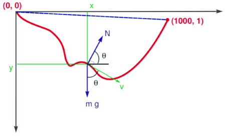
Although the concepts of designer units, scaling and balancing have been used for more than a decade to generate successful flight and field operations[9, 10, 11, 12, 14, 17, 20], the process has largely been ad hoc until recently. Because the flight problems are too involved for illustrating the procedures, we design a far simpler problem that typifies the systematic process of scaling and balancing. To this end, consider the well-known Brachistochrone problem. Instead of using well-scaled numbers as is customarily discussed in many textbooks, we purposefully choose the final-time condition on the position coordinates (x,y)𝑥𝑦(x,y) to be widely disparate and given by (1000,1)10001(1000,1) meters; see Fig. 1. This results in a badly-scaled or “bad” Brachistochrone problem that can be formulated as[4],

𝕏=3𝕌=𝒙=(x,y,v)𝒖=θ}(preamble)\left.\begin{aligned} \hskip 22.76228pt\phantom{\quad\textsf{(preamble)}}\mathbb{X}&={\mathbb{R}}^{3}&\mathbb{U}&=\mathbb{R}&\\ \boldsymbol{x}&=(x,y,v)\quad&{\boldsymbol{u}}&=\theta&\\ \end{aligned}\hskip 34.14322pt\right\}\hskip 8.5359pt\text{(preamble)}
(BR){Minimize J[𝒙(),𝒖(),tf]=tf}(cost)Subject tox˙=vsinθy˙=vcosθv˙=gcosθ}(dynamics)(t0,x0,y0,v0)=(0,0,0,0)(xf,yf)=(1000,1)}(endpoints)\displaystyle(B_{R})\left\{\begin{array}[]{ll}\text{Minimize }&\left.\begin{aligned} \makebox[58.66475pt][r]{$\displaystyle J[\boldsymbol{x}(\cdot),{\boldsymbol{u}}(\cdot),t_{f}]$}&=\makebox[43.88902pt][l]{$\displaystyle t_{f}$}\\ \end{aligned}\right\}\quad\,\text{(cost)}\\[6.99997pt] \text{Subject to}&\\[-15.00002pt] &\left.\begin{aligned} \makebox[58.66475pt][r]{$\displaystyle\dot{x}$}&=\makebox[43.88902pt][l]{$\displaystyle v\sin\theta$}\\ \dot{y}&=v\cos\theta\\ \dot{v}&=g\cos\theta\end{aligned}\right\}\quad\text{(dynamics)}\\ &\left.\begin{aligned} \makebox[58.66475pt][r]{$\displaystyle(t_{0},x_{0},y_{0},v_{0})$}&=\makebox[43.88902pt][l]{$\displaystyle(0,0,0,0)$}\\ (x_{f},y_{f})&=(1000,1)\end{aligned}\right\}\quad\text{(endpoints)}\end{array}\right.

where, g=9.8meters/sec2𝑔9.8meterssuperscriptsec2g=9.8\ \textit{meters}/\textit{sec}^{2}. See Fig. 1 for a physical definition of the variables.
Refer to caption
Figure 1: Schematic for the “bad” Brachistochrone problem. Figure is not to scale.

6.1 Illustrating the Process for Choosing Designer Units

As a consequence of (24i), we can write,

𝒙:=[xyv]x-unitsy-unitsv-unitsassign𝒙delimited-[]𝑥𝑦𝑣𝑥-units𝑦-units𝑣-units\boldsymbol{x}:=\left[\begin{array}[]{c}x\\ y\\ v\end{array}\right]\ \begin{array}[]{c}x\text{-units}\\ y\text{-units}\\ v\text{-units}\end{array} (29)

Because the cost unit is the same as the time unit, the adjoint covector is defined by

𝝀:=[λxλyλv]t-units/x-unitst-units/y-unitst-units/v-unitsassign𝝀delimited-[]subscript𝜆𝑥subscript𝜆𝑦subscript𝜆𝑣𝑡-units𝑥-units𝑡-units𝑦-units𝑡-units𝑣-units{\mbox{\boldmath$\lambda$}}:=\left[\begin{array}[]{c}\lambda_{x}\\ \lambda_{y}\\ \lambda_{v}\end{array}\right]\ \begin{array}[]{c}t\text{-units}/x\text{-units}\\ t\text{-units}/y\text{-units}\\ t\text{-units}/v\text{-units}\end{array} (30)

As a result, the Hamiltonian

H(𝝀,𝒙,𝒖)=λxvsinθ+λyvcosθ+λvgcosθ𝐻𝝀𝒙𝒖subscript𝜆𝑥𝑣𝜃subscript𝜆𝑦𝑣𝜃subscript𝜆𝑣𝑔𝜃H({\mbox{\boldmath$\lambda$}},\boldsymbol{x},{\boldsymbol{u}})=\lambda_{x}v\sin\theta+\lambda_{y}v\cos\theta+\lambda_{v}g\cos\theta (31)

is dimensionless.

Applying the Hamiltonian minimization condition, we get

λx(t)v(t)cosθ(t)λy(t)v(t)sinθ(t)λv(t)gsinθ(t)=0(t[t0,tf])subscript𝜆𝑥𝑡𝑣𝑡𝜃𝑡subscript𝜆𝑦𝑡𝑣𝑡𝜃𝑡subscript𝜆𝑣𝑡𝑔𝜃𝑡0for-all𝑡subscript𝑡0subscript𝑡𝑓\lambda_{x}(t)v(t)\cos\theta(t)-\lambda_{y}(t)v(t)\sin\theta(t)-\lambda_{v}(t)g\sin\theta(t)=0\quad(\forall\ t\in[t_{0},t_{f}]) (32)

The adjoint equations,

λ˙x=subscript˙𝜆𝑥absent\displaystyle\dot{\lambda}_{x}= 00\displaystyle 0 (33)
λ˙y=subscript˙𝜆𝑦absent\displaystyle\dot{\lambda}_{y}= 00\displaystyle 0
λ˙v=subscript˙𝜆𝑣absent\displaystyle\dot{\lambda}_{v}= λxsinθλycosθsubscript𝜆𝑥𝜃subscript𝜆𝑦𝜃\displaystyle-\lambda_{x}\sin\theta-\lambda_{y}\cos\theta

indicate that λxsubscript𝜆𝑥\lambda_{x} and λysubscript𝜆𝑦\lambda_{y} are constants. In addition, the transversality condition,

λv(tf)=0subscript𝜆𝑣subscript𝑡𝑓0\lambda_{v}(t_{f})=0 (34)

and the Hamiltonian value condition,

H[@tf]:=λx(tf)v(tf)sinθ(tf)+λy(tf)v(tf)cosθ(tf)+λv(tf)gcosθ(tf)=1assign𝐻delimited-[]@subscript𝑡𝑓subscript𝜆𝑥subscript𝑡𝑓𝑣subscript𝑡𝑓𝜃subscript𝑡𝑓subscript𝜆𝑦subscript𝑡𝑓𝑣subscript𝑡𝑓𝜃subscript𝑡𝑓subscript𝜆𝑣subscript𝑡𝑓𝑔𝜃subscript𝑡𝑓1H[@t_{f}]:=\lambda_{x}(t_{f})v(t_{f})\sin\theta(t_{f})+\lambda_{y}(t_{f})v(t_{f})\cos\theta(t_{f})+\lambda_{v}(t_{f})g\cos\theta(t_{f})=-1 (35)

complete the computational set of conditions that define the boundary value problem. These equations can also be used as part of the totality of a verification and validation of a candidate optimal solution obtained by any computational method.

In order to perform initial scaling, we simply take the given numerical data as a starting point. For the numerics given in Problem BRsubscript𝐵𝑅B_{R}, we expect x𝑥x to satisfy,

0x10000𝑥10000\leq x\leq 1000 (36)

In the absence of further analysis, we can assume y𝑦y to take on similar range of values. Furthermore, because the x𝑥x-distance is relatively large, we expect the time of travel to be relatively large (in terms of seconds). Based on these heuristics, we choose an initial set of scaling factors according to:

x𝑥\displaystyle x =Pxx~absentsubscript𝑃𝑥~𝑥\displaystyle=P_{x}\ \widetilde{x} =100x~absent100~𝑥\displaystyle=100\ \widetilde{x} (37)
y𝑦\displaystyle y =Pyy~absentsubscript𝑃𝑦~𝑦\displaystyle=P_{y}\ \widetilde{y} =20y~absent20~𝑦\displaystyle=20\ \widetilde{y}
v𝑣\displaystyle v =Pvv~absentsubscript𝑃𝑣~𝑣\displaystyle=P_{v}\ \widetilde{v} =10v~absent10~𝑣\displaystyle=10\ \widetilde{v}
θ𝜃\displaystyle\theta =Pθθ~absentsubscript𝑃𝜃~𝜃\displaystyle=P_{\theta}\ \widetilde{\theta} =θ~absent~𝜃\displaystyle=\widetilde{\theta}
t𝑡\displaystyle t =ptt~absentsubscript𝑝𝑡~𝑡\displaystyle=p_{t}\ \widetilde{t} =10t~absent10~𝑡\displaystyle=10\ \widetilde{t}

As a result of (37), the large variation in x𝑥x indicated by (36) is tempered by x~~𝑥\widetilde{x} according to

0x~100~𝑥100\leq\widetilde{x}\leq 10

Note that the numbers given in (37) imply a unit of distance along the x𝑥x-axis that is completely different from the unit of distance along the y𝑦y axis! In fact, these numbers constitute a specific system of units that do not conform with the metric system or any other set of the standard units; hence, these are designer units. The conversion between the designer units of (37) and the metric units is given by,

1x~-unit1~𝑥-unit\displaystyle 1\ \widetilde{x}\text{-unit} =1 unit of distance along x-axisabsent1 unit of distance along x-axis\displaystyle=\text{1 unit of distance along $x$-axis} =100 metersabsent100 meters\displaystyle=100\text{ meters} (38)
1y~-unit1~𝑦-unit\displaystyle 1\ \widetilde{y}\text{-unit} =1 unit of distance along y-axisabsent1 unit of distance along y-axis\displaystyle=\text{1 unit of distance along $y$-axis} =20 metersabsent20 meters\displaystyle=20\text{ meters}
1v~-unit1~𝑣-unit\displaystyle 1\ \widetilde{v}\text{-unit} =1 unit of speedabsent1 unit of speed\displaystyle=\text{1 unit of speed} =10 meters/secondabsent10 meters/second\displaystyle=10\text{ meters/second}
1t~-unit1~𝑡-unit\displaystyle 1\ \widetilde{t}\text{-unit} =1 unit of timeabsent1 unit of time\displaystyle=\text{1 unit of time } =10 secondsabsent10 seconds\displaystyle=10\text{ seconds}

It is important to note that the velocity unit is completely independent of any of the x𝑥x, y𝑦y or t𝑡t units. Consequently, these designer units are not consistent in the sense that,

dy~dt~v~cosθ~𝑑~𝑦𝑑~𝑡~𝑣~𝜃\frac{d\widetilde{y}}{d\widetilde{t}}\neq\widetilde{v}\cos\widetilde{\theta}

To drive home this point, we note that we can no longer express g𝑔g in terms of distance units per the square of time units. For instance, in the metric system, the unit of g𝑔g is given by meters/sec2meterssuperscriptsec2\textit{meters}/\textit{sec}^{2}. Because we chose distance units along the x𝑥x- and y𝑦y-directions to be independent of each other, it is clear that that we cannot regard g𝑔g in terms of “distance units per the square of time units.” The proper unit for g𝑔g is obtained by considering dv~/dt~𝑑~𝑣𝑑~𝑡d\widetilde{v}/d\widetilde{t}. This implies that we may regard the gravitational acceleration as being transformed according to

g~=(ptPv)g=9.8v~-unit/t~-unit~𝑔subscript𝑝𝑡subscript𝑃𝑣𝑔9.8~𝑣-unit~𝑡-unit\widetilde{g}=\left(\frac{p_{t}}{P_{v}}\right)g=9.8\ \widetilde{v}\text{-unit}/\widetilde{t}\text{-unit} (39)

That is, g~1~𝑔1\widetilde{g}\neq 1 numerically, which is a typical number for canonical units[3]. That g~=g~𝑔𝑔\widetilde{g}=g numerically in (39) is simply coincidental and as a result of choosing pt=Pvsubscript𝑝𝑡subscript𝑃𝑣p_{t}=P_{v} in (37).

Using the scaling units of (37) the endpoint conditions can be written as,

t~0subscript~𝑡0\displaystyle\widetilde{t}_{0} =0absent0\displaystyle=0 (in t~-units)in ~𝑡-units\displaystyle(\text{in }\widetilde{t}\text{-units}) (40)
x~(t~0)~𝑥subscript~𝑡0\displaystyle\widetilde{x}(\widetilde{t}_{0}) =0absent0\displaystyle=0 x~(t~f)~𝑥subscript~𝑡𝑓\displaystyle\widetilde{x}(\widetilde{t}_{f}) =10absent10\displaystyle=10 (in x~-units)in ~𝑥-units\displaystyle(\text{in }\widetilde{x}\text{-units})
y~(t~0)~𝑦subscript~𝑡0\displaystyle\widetilde{y}(\widetilde{t}_{0}) =0absent0\displaystyle=0 y~(t~f)~𝑦subscript~𝑡𝑓\displaystyle\widetilde{y}(\widetilde{t}_{f}) =0.05absent0.05\displaystyle=0.05\qquad (in y~-units)in ~𝑦-units\displaystyle(\text{in }\widetilde{y}\text{-units})
v~0subscript~𝑣0\displaystyle\widetilde{v}_{0} =0absent0\displaystyle=0 (in v~-units)in ~𝑣-units\displaystyle(\text{in }\widetilde{v}\text{-units})

Imposing the endpoint conditions according to (40) is tantamount to choosing 𝑷esubscript𝑷𝑒{\boldsymbol{P}}_{e} according to,

𝑷e=diag(10,100,100,20,20,10)subscript𝑷𝑒diag10100100202010{\boldsymbol{P}}_{e}=\textrm{diag}(10,100,100,20,20,10) (41)

This follows as a direct consequence of (37). Finally, we scale the cost functional using pJ=10subscript𝑝𝐽10p_{J}=10 so that we can write,

J~[𝒙~(),𝒖~(),t~0,t~f]=t~f~𝐽~𝒙~𝒖subscript~𝑡0subscript~𝑡𝑓subscript~𝑡𝑓\widetilde{J}[{\widetilde{\boldsymbol{x}}}(\cdot),{\widetilde{{\boldsymbol{u}}}}(\cdot),\widetilde{t}_{0},\widetilde{t}_{f}]=\widetilde{t}_{f}

At this juncture, we wish to emphasize that the purpose of initial scaling is not necessarily to generate the best set of designer units; rather, it is largely directed at producing a work-flow for balancing. As will be apparent shortly, once an initial numerical result is obtained, balancing can usually be performed in just about two iterations. One situation when initial scaling becomes critical to the work-flow is when no numerical result is achieved simply because of poor scaling. The detection and mitigation of this problem are open areas of research.

6.2 Illustrating the Process of Descaling the Covectors

For the purposes of clarity of the discussions to follow, we use the following terminology:

  1. 1.

    Unscaled: This refers to all numbers and variables associated with the original (or unscaled) problem.

  2. 2.

    Scaled: This refers to all numbers and variables associated with the affinely transformed (or scaled) problem.

  3. 3.

    Descaled: This refers to all numbers and variables that are purported solutions to the unscaled problem obtained via (22) and a solution to the scaled problem.

Applying (22) to descale the adjoint covector, we get,

λxsubscript𝜆𝑥\displaystyle\lambda_{x} =λ~x(pJPx)absentsubscript~𝜆𝑥subscript𝑝𝐽subscript𝑃𝑥\displaystyle=\widetilde{\lambda}_{x}\left(\frac{p_{J}}{P_{x}}\right) =\displaystyle= λ~x10subscript~𝜆𝑥10\displaystyle\frac{\widetilde{\lambda}_{x}}{10} (secondsmeters)secondsmeters\displaystyle\left(\frac{\text{seconds}}{\text{meters}}\right) (42)
λysubscript𝜆𝑦\displaystyle\lambda_{y} =λ~y(pJPy)absentsubscript~𝜆𝑦subscript𝑝𝐽subscript𝑃𝑦\displaystyle=\widetilde{\lambda}_{y}\left(\frac{p_{J}}{P_{y}}\right) =\displaystyle= λ~y2subscript~𝜆𝑦2\displaystyle\frac{\widetilde{\lambda}_{y}}{2} (secondsmeters)secondsmeters\displaystyle\left(\frac{\text{seconds}}{\text{meters}}\right)
λvsubscript𝜆𝑣\displaystyle\lambda_{v} =λ~v(pJPv)absentsubscript~𝜆𝑣subscript𝑝𝐽subscript𝑃𝑣\displaystyle=\widetilde{\lambda}_{v}\left(\frac{p_{J}}{P_{v}}\right) =\displaystyle= λ~vsubscript~𝜆𝑣\displaystyle\widetilde{\lambda}_{v} (seconds2meters)superscriptseconds2meters\displaystyle\left(\frac{\text{seconds}^{2}}{\text{meters}}\right)

Similarly, from (41) and (21) we have

𝑷ν=10[𝑷e1]T(νt0,νx0,νxf,νy0,νyf,νv0)=(ν~t0,ν~x010,ν~xf10,ν~y02,ν~yf2,ν~v0)subscript𝑷𝜈10superscriptdelimited-[]superscriptsubscript𝑷𝑒1𝑇subscript𝜈subscript𝑡0subscript𝜈subscript𝑥0subscript𝜈subscript𝑥𝑓subscript𝜈subscript𝑦0subscript𝜈subscript𝑦𝑓subscript𝜈subscript𝑣0subscript~𝜈subscript𝑡0subscript~𝜈subscript𝑥010subscript~𝜈subscript𝑥𝑓10subscript~𝜈subscript𝑦02subscript~𝜈subscript𝑦𝑓2subscript~𝜈subscript𝑣0{\boldsymbol{P}}_{\nu}=10\left[{\boldsymbol{P}}_{e}^{-1}\right]^{T}\Rightarrow(\nu_{t_{0}},\nu_{x_{0}},\nu_{x_{f}},\nu_{y_{0}},\nu_{y_{f}},\nu_{v_{0}})=\left(\widetilde{\nu}_{t_{0}},\frac{\widetilde{\nu}_{x_{0}}}{10},\frac{\widetilde{\nu}_{x_{f}}}{10},\frac{\widetilde{\nu}_{y_{0}}}{2},\frac{\widetilde{\nu}_{y_{f}}}{2},\widetilde{\nu}_{v_{0}}\right) (43)

where, ν𝜈\nu and ν~~𝜈\widetilde{\nu} with the appropriate subscripts are the endpoint multipliers associated with the initial and final-time conditions. Note that these endpoint multipliers also have units similar to those identified in (42).

6.3 Illustrating the Numerical Process of Scaling and Balancing

All of the analysis so far has been agnostic to the specific choice of a numerical method or software. To demonstrate the numerical process, any appropriate mathematical software may be used. We begin by choosing DIDO©, a state-of-the-art MATLAB® toolbox for solving optimal control problems[4]. DIDO is the same tool that was used in all of the flight applications noted earlier. It is based on the the spectral algorithm[25, 26, 27, 28, 29, 30] for pseudospectral optimal control and does not require any guess of the solution to solve the problem. Furthermore, DIDO automatically generates all of the covectors associated with a generic optimal control problem (see Problem Bλsuperscript𝐵𝜆B^{\lambda} presented in Section II of this paper) through an implementation of the Covector Mapping Principle[4, 20, 30]. That is, DIDO generates a guess-free candidate solution to the BVP while only requiring the data functions for Problem B𝐵B. This is why the spectral algorithm and its implementation in DIDO do not belong to the class of “direct” or “indirect” methods. In fact, these ideas effectively obviate the need for such a classification; see Sec. 2.9.2 of Ref. [4].

6.3.1 Initial Scaling and Descaling

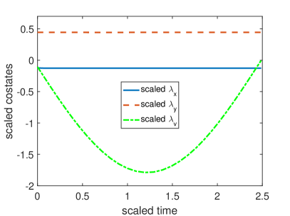
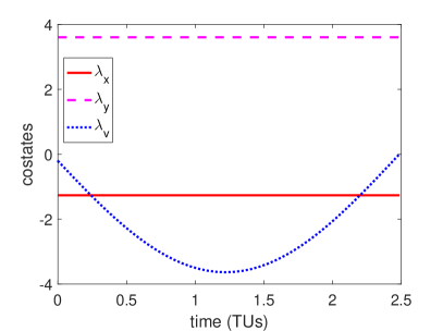
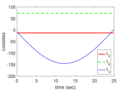
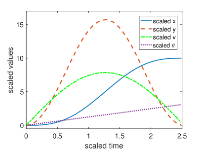
A candidate primal-dual solution (generated by DIDO) is shown in Fig. 2.
Refer to caption
Refer to caption
Figure 2: Guess-free primal (left) and dual (right) solutions to the badly-scaled Brachistochrone problem.

By definition, these are simply candidate solutions to the scaled problem. They have not yet been validated. Because it is frequently more meaningful to validate results in physical units, we first descale the primal variables using (37). The descaled candidate control trajectory is then used to propagate the initial conditions,

x(0)=0,y(0)=0,v(0)=0formulae-sequence𝑥00formulae-sequence𝑦00𝑣00x(0)=0,\quad y(0)=0,\quad v(0)=0

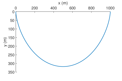
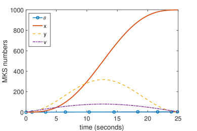
using linear interpolation for the controls and ode45 in MATLAB. The propagated state trajectory is shown in Fig. 3.
Refer to caption
Refer to caption
Figure 3: Primal feasible solution to the badly-scaled Brachistochrone problem indicating variations in three-orders of magnitude.

The propagated values of x(tf)𝑥subscript𝑡𝑓x(t_{f}) and y(tf)𝑦subscript𝑡𝑓y(t_{f}) satisfy the final-time conditions to the following precision,

x(tf)1000=3.6×10³m,y(tf)1=1.9×10⁴mformulae-sequencedelimited-∣∣𝑥subscript𝑡𝑓10003.6superscript103𝑚delimited-∣∣𝑦subscript𝑡𝑓11.9superscript104𝑚\mid x(t_{f})-1000\mid=3.6\times 10^{-3}\ m,\quad\mid y(t_{f})-1\mid=1.9\times 10^{-4}\ m

Thus, the descaled solution is verifiably feasible. In flight applications, such an independent verification of feasibility is critical to a successful pre-flight checkout[12, 14, 20].

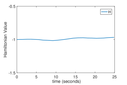
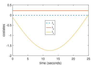
To validate the extremality of the feasible solution, we use (42) and (23) to descale the adjoint covectors and the evolution of the Hamiltonian respectively. The results are shown in Fig. 4.
Refer to caption
Refer to caption
Figure 4: Descaled costates and the evolution of the Hamiltonian for the badly-scaled Brachistochrone problem.

It is apparent that λx(t)subscript𝜆𝑥𝑡\lambda_{x}(t) and λy(t)subscript𝜆𝑦𝑡\lambda_{y}(t) are constants as required by (33). It is also apparent that the Hamiltonian is nearly a constant and equal to 11-1 as required by (35) and the first integral. Thus, the theoretical necessary conditions are satisfied up to the indicated approximations.111Although the spectral algorithm can theoretically generate very accurate solutions[4, 20, 28, 30], the Hamiltonian evolution equation is satisfied only weakly[36]; hence, the Hamiltonian is not expected to be equal to 11-1 in the strong Lsubscript𝐿L_{\infty}-norm in Fig. 4. In addition, because no Jacobian information was provided in the generation of Fig. 4, the accuracy in the computation of the dual variables is expected to be lower than that of the primal solution. Note also that dual (or primal) tolerances cannot be set to arbitrarily small numbers (e.g., 106superscript10610^{-6} or 108superscript10810^{-8}) to attain “higher accuracy” because they may violate consistency conditions[31]. See [32] for details and [33] for a unified framework. These indicators of optimality validate that the solution presented in Fig. 2 is at least an extremal.

6.3.2 Illustrating Universality of Proposition A𝐴A

To illustrate that Proposition A𝐴A is indeed universal (and not merely specific to DIDO), we construct a shooting algorithm using ode45 and fsolve from the MATLAB optimization toolbox. The objective of ode45 is to generate the vector function,

𝐒:(λx0,λy0,λv0,tf)(xf,yf,vf,Hf):𝐒maps-tosubscript𝜆subscript𝑥0subscript𝜆subscript𝑦0subscript𝜆subscript𝑣0subscript𝑡𝑓subscript𝑥𝑓subscript𝑦𝑓subscript𝑣𝑓subscript𝐻𝑓\mathbf{S}:(\lambda_{x_{0}},\lambda_{y_{0}},\lambda_{v_{0}},t_{f})\mapsto(x_{f},y_{f},v_{f},H_{f}) (44)

by integrating the six state-costate equations using the initial conditions (at t0=0subscript𝑡00t_{0}=0),

x(t0)=0,y(t0)=0,v(t0)=0,λx(t0)=λx0,λy(t0)=λy0,λv(t0)=λv0formulae-sequence𝑥subscript𝑡00formulae-sequence𝑦subscript𝑡00formulae-sequence𝑣subscript𝑡00formulae-sequencesubscript𝜆𝑥subscript𝑡0subscript𝜆subscript𝑥0formulae-sequencesubscript𝜆𝑦subscript𝑡0subscript𝜆subscript𝑦0subscript𝜆𝑣subscript𝑡0subscript𝜆subscript𝑣0x(t_{0})=0,y(t_{0})=0,v(t_{0})=0,\lambda_{x}(t_{0})=\lambda_{x_{0}},\lambda_{y}(t_{0})=\lambda_{y_{0}},\lambda_{v}(t_{0})=\lambda_{v_{0}}

The quantity Hfsubscript𝐻𝑓H_{f} in (44) is the final value of the Hamiltonian evaluated using the results of the integration and (31). The objective of fsolve is to solve for the zeros of the residual vector function 𝒓:44:𝒓superscript4superscript4{\boldsymbol{r}}:{\mathbb{R}}^{4}\rightarrow{\mathbb{R}}^{4} defined by,

𝒓(λx0,λy0,λv0,tf):=S(λx0,λy0,λv0,tf)(1000101)assign𝒓subscript𝜆subscript𝑥0subscript𝜆subscript𝑦0subscript𝜆subscript𝑣0subscript𝑡𝑓Ssubscript𝜆subscript𝑥0subscript𝜆subscript𝑦0subscript𝜆subscript𝑣0subscript𝑡𝑓1000101{\boldsymbol{r}}(\lambda_{x_{0}},\lambda_{y_{0}},\lambda_{v_{0}},t_{f}):=\textbf{S}(\lambda_{x_{0}},\lambda_{y_{0}},\lambda_{v_{0}},t_{f})-\left(\begin{array}[]{c}1000\\ 1\\ 0\\ -1\\ \end{array}\right) (45)

Because a shooting algorithm is fundamentally doomed by the curse of sensitivity[4], we choose the values of the guess to be almost exactly equal to the expected solution,

λx0=0.013,λy0=0.225,λv0=0.113,tf=24.0formulae-sequencesubscript𝜆subscript𝑥00.013formulae-sequencesubscript𝜆subscript𝑦00.225formulae-sequencesubscript𝜆subscript𝑣00.113subscript𝑡𝑓24.0\lambda_{x_{0}}=-0.013,\quad\lambda_{y_{0}}=0.225,\quad\lambda_{v_{0}}=-0.113,\quad t_{f}=24.0 (46)

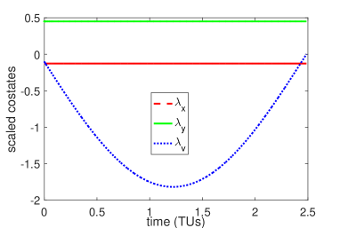
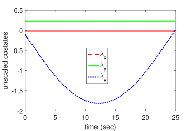
For the purposes of brevity, we limit our discussions to only the costate trajectories. Shown in Fig. 5 are both the unscaled and scaled costates trajectories obtained by the shooting algorithm.
Refer to caption
Refer to caption
Figure 5: Unscaled and scaled costates obtained by a shooting method for the badly-scaled Brachistochrone problem.

The scaled costates were obtained by using the scaled equations and replacing the numerical value of the 4-vector in (45) by its scaled counterpart (see (40)). It is apparent that the unscaled costates match the descaled costates (see Fig. 4) and the scaled costates match the DIDO result shown in Fig. 2 to numerical precision. In other words, we have demonstrated that Proposition A is independent of the numerical algorithm or software.

6.3.3 Illustrating a Process for Better Balancing

As a final point of illustration, we now demonstrate that it is possible to achieve a more balanced computational optimal control problem. First, note from the range of values of the ordinates in Fig. 2, that the computational problem is not perfectly balanced. This is precisely what happens in solving many flight application problems; that is, it is frequently not possible to choose designer units that achieve well-balanced equations at the first attempt. Nonetheless, after further analysis of the type illustrated in the preceding paragraphs, it is possible to achieve a better balanced computational problem by merely inspecting the results. Based on the range of values indicated in Fig. 2, we now rescale the primal problem using the following units:

x𝑥\displaystyle x =Pxx~absentsubscript𝑃𝑥~𝑥\displaystyle=P_{x}\ \widetilde{x} =1000x~absent1000~𝑥\displaystyle=1000\ \widetilde{x} 1 distance unit along x-axisabsent1 distance unit along x-axis\displaystyle\Rightarrow\text{1 distance unit along $x$-axis} =1000 metersabsent1000 meters\displaystyle=1000\text{ meters} (47)
y𝑦\displaystyle y =Pyy~absentsubscript𝑃𝑦~𝑦\displaystyle=P_{y}\ \widetilde{y} =160y~absent160~𝑦\displaystyle=160\ \widetilde{y} 1 distance unit along y-axisabsent1 distance unit along y-axis\displaystyle\Rightarrow\text{1 distance unit along $y$-axis} =160 metersabsent160 meters\displaystyle=160\text{ meters}
v𝑣\displaystyle v =Pvv~absentsubscript𝑃𝑣~𝑣\displaystyle=P_{v}\ \widetilde{v} =20v~absent20~𝑣\displaystyle=20\ \widetilde{v} 1 speed unitabsent1 speed unit\displaystyle\Rightarrow\text{1 speed unit } =20 meters/secondabsent20 meters/second\displaystyle=20\text{ meters/second}

All other choices of units are the same as before; see (37). Clearly, x~2+y~2superscript~𝑥2superscript~𝑦2\sqrt{\widetilde{x}^{2}+\widetilde{y}^{2}} is meaningless. Note also that the numerical choice of these scaling factors further the disparity between the new set of designer units and the original physical units. For instance, the gravitational acceleration transforms according to

g~=(ptPv)g=4.9v~-unit/t~-unit~𝑔subscript𝑝𝑡subscript𝑃𝑣𝑔4.9~𝑣-unit~𝑡-unit\widetilde{g}=\left(\frac{p_{t}}{P_{v}}\right)g=4.9\ \widetilde{v}\text{-unit}/\widetilde{t}\text{-unit} (48)

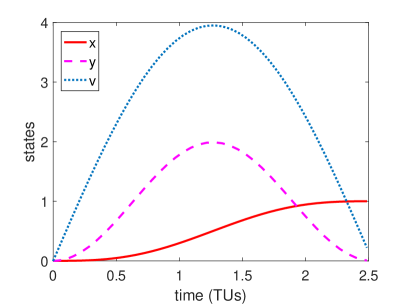
The primal and dual trajectories for the rescaled problem are shown in Fig. 6.
Refer to caption
Refer to caption
Figure 6: Rescaled solution to the badly-scaled Brachistochrone problem obtained by using the better-balanced set of designer units given by (47).

By inspection, it is clear that the problem is reasonably well-balanced with all variables contained in the range [4,4]44[-4,4].

6.3.4 Illustrating the Fallacy of Balancing on the Unit Interval

Suppose we scale the primal problem using the following designer units:

x𝑥\displaystyle x =Pxx~absentsubscript𝑃𝑥~𝑥\displaystyle=P_{x}\ \widetilde{x} =1000x~absent1000~𝑥\displaystyle=1000\ \widetilde{x} (49)
y𝑦\displaystyle y =Pyy~absentsubscript𝑃𝑦~𝑦\displaystyle=P_{y}\ \widetilde{y} =320y~absent320~𝑦\displaystyle=320\ \widetilde{y}
v𝑣\displaystyle v =Pvv~absentsubscript𝑃𝑣~𝑣\displaystyle=P_{v}\ \widetilde{v} =80v~absent80~𝑣\displaystyle=80\ \widetilde{v}
t𝑡\displaystyle t =ptt~absentsubscript𝑝𝑡~𝑡\displaystyle=p_{t}\ \widetilde{t} =t~absent~𝑡\displaystyle=\widetilde{t}

A quick examination of Fig. 3 shows that (49) will force all the state variables to lie on the unit interval [0,1]01[0,1]. That this is indeed the case is shown in Fig. 7.
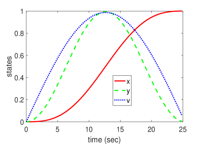
Refer to caption
Refer to caption
Figure 7: Primal-normalized solution to the badly-scaled Brachistochrone problem obtained by using the set of designer units given by (49).

Also shown in Fig. 7 are the corresponding costates. As expected (by Proposition A𝐴A and by inspection of Fig. 4) the dual variables now lie in the range [200,100]200100[-200,100]. In this particular situation, the range [200,100]200100[-200,100] is only about two orders of magnitude away from the desirable interval of [1,1]11[-1,1]; hence, it is no cause for serious alarm. Nonetheless, it is apparent that the imbalance may be greater in other applications.

In certain applications, the state variables may be naturally constrained to lie on the unit interval (e.g., quaternion parametrization). If the costates (e.g., co-quaternions) are imbalanced, it is still possible to balance the state-costate pair by scaling the states to lie on a non-unit interval through a proper selection of 𝑷xsubscript𝑷𝑥{\boldsymbol{P}}_{x} in Proposition A𝐴A. In other words, there is no real reason to be constrained on a unit interval. In stronger terms, the conventional wisdom of scaling on a unit interval is not necessarily the best approach to balancing optimal control problems.

7 Adjunct Consequences of Scaling and Balancing

The consequences of scaling and balancing go far beyond faster computation of optimal trajectories. When the pseudospectral optimal control method of the early days[34, 35, 36, 37, 38, 39, 40] (c. 1995 - c. 2005) is applied to solve the bad Brachistochrone problem; i.e., without using proper scaling or spectral techniques[25, 28, 30], the approach fails to produce the correct solution. In general, the same is true of Runge-Kutta collocation methods; see [31] and [41]. If an algorithm does not generate a feasible solution to a problem with a known solution – such as the Brachistochrone problem – then it is a clear failure of the algorithm. Frequently, we use optimal control techniques to solve “hard” problems where we do not know in advance if a solution exists. In such practical situations it is important to know if the lack of a feasible solution is due to a failure of the algorithm or a genuine non-existence of a solution. Consequently, over the last decade, proper scaling and balancing have been fundamentally intertwined with the theory and practice of optimal control[1, 4, 9, 11, 13, 14].

7.1 Feasibility via Optimization

In many practical applications, there is a need to simply generate feasible solutions. Consequently, scaling and balancing techniques are critical not only for faster optimization but also to answer the more fundamental and difficult theoretical question[23] of the existence of a solution.

As a means to illustrate this aspect of the intertwining between theory and practice, consider the optimal propellant maneuver (OPM) that is actively used[9] in current flight operations of the International Space Station (ISS). The OPM saves NASA 90%percent9090\% propellant in momentum management at a savings of approximately $ 1,000,000 per maneuver[9, 10, 12]. This maneuver was designed by Bedrossian after his discovery of the zero propellant maneuver (ZPM) that saves all 100%percent100100\% of propellant[11]. Prior to Bedrossian’s discovery, it was generally thought that it was impossible to dump all of the accumulated momentum without any propellant consumption[42]. In other words, a feasible solution (for 100%percent100100\% propellant savings) was believed to be nonexistent. When the “unscaled” values of the ISS angular momentum, hh, the control torque u𝑢u, and angular velocity ω𝜔\omega are used for dynamic optimization, all prior methods investigated by Bedrossian et al consistently failed to generate a feasible solution. These variables vary as[11]:

104superscript104\displaystyle-10^{4} h104absentsuperscript104\displaystyle\leq h\leq 10^{4} lb-ft-s
102superscript102\displaystyle-10^{2} u102absent𝑢superscript102\displaystyle\leq u\leq 10^{2} lb-ft
104superscript104\displaystyle-10^{-4} ω104absent𝜔superscript104\displaystyle\leq\omega\leq 10^{-4} s1superscript𝑠1\displaystyle s^{-1}

Consequently, a failure to find a feasible zero-propellant solution was consistent with the pre-ZPM belief of physics. Were it not for proper scaling and balancing, the ZPM might have gone undiscovered. More specifically, when the variables are transformed according to

h\displaystyle h =1000h~absent1000~\displaystyle=1000\ \widetilde{h} lb-ft-s (50)
u𝑢\displaystyle u =10u~absent10~𝑢\displaystyle=10\ \widetilde{u} lb-ft
t𝑡\displaystyle t =1000t~absent1000~𝑡\displaystyle=1000\ \widetilde{t} s𝑠\displaystyle s

not only were Bedrossian et al[11] able to find a feasible solution but also several different solutions! In other words, a special choice of designer units “converted” a hard problem to an easy one. The rest is history[10].

The lessons learned from such successes and similar ones that followed[9, 14, 15, 16, 17] are codified in the scaling and balancing techniques presented in the preceding sections. More specifically, the last decade has witnessed the use theoretical optimization principles to determine the practical feasibility of innovative concepts as opposed to the more conventional use of algorithms to optimize a feasible design. In other words, optimal control theory has been used a tool to innovate and not merely to optimize.

7.2 Nonuniqueness of the Costates

Note that Proposition A only asserts the existence of linearly descaled covectors; it does not imply uniqueness. Using the same arguments as that of Proposition A, it is relatively straightforward to show that the costates in an optimal control problem are not necessarily unique. This is achieved by replacing the linear equations (22d)-(22f) with its affine counterparts:

𝝀():=assignsuperscript𝝀absent\displaystyle{\mbox{\boldmath$\lambda$}}^{*}(\cdot):= 𝑷λ𝝀~()+𝒒λ()subscript𝑷𝜆superscriptbold-~𝝀subscript𝒒𝜆\displaystyle{\boldsymbol{P}}_{\lambda}\ {\mbox{\boldmath$\widetilde{\lambda}$}}^{*}(\cdot)+{\boldsymbol{q}}_{\lambda}(\cdot) (51a)
𝝁():=assignsuperscript𝝁absent\displaystyle{\mbox{\boldmath$\mu$}}^{*}(\cdot):= 𝑷μ𝝁~()+𝒒μ()subscript𝑷𝜇superscriptbold-~𝝁subscript𝒒𝜇\displaystyle{\boldsymbol{P}}_{\mu}\ {\mbox{\boldmath$\widetilde{\mu}$}}^{*}(\cdot)+{\boldsymbol{q}}_{\mu}(\cdot) (51b)
𝝂:=assignsuperscript𝝂absent\displaystyle{\mbox{\boldmath$\nu$}}^{*}:= 𝑷ν𝝂~+𝒒νsubscript𝑷𝜈superscriptbold-~𝝂subscript𝒒𝜈\displaystyle{\boldsymbol{P}}_{\nu}\ {\mbox{\boldmath$\widetilde{\nu}$}}^{*}+{\boldsymbol{q}}_{\nu} (51c)

where, 𝒒λ():tNx:subscript𝒒𝜆maps-to𝑡superscriptsubscript𝑁𝑥{\boldsymbol{q}}_{\lambda}(\cdot):t\mapsto{\mathbb{R}}^{N_{x}}, 𝒒μ():tNh:subscript𝒒𝜇maps-to𝑡superscriptsubscript𝑁{\boldsymbol{q}}_{\mu}(\cdot):t\mapsto{\mathbb{R}}^{N_{h}} and 𝒒νNesubscript𝒒𝜈superscriptsubscript𝑁𝑒{\boldsymbol{q}}_{\nu}\in{\mathbb{R}}^{N_{e}}. Obviously, 𝒒λ()𝟎subscript𝒒𝜆0{\boldsymbol{q}}_{\lambda}(\cdot)\equiv{\bf 0}, 𝒒μ()𝟎subscript𝒒𝜇0{\boldsymbol{q}}_{\mu}(\cdot)\equiv{\bf 0} and 𝒒ν=𝟎subscript𝒒𝜈0{\boldsymbol{q}}_{\nu}={\bf 0} recovers Proposition A; however, by substituting (51) in Problem Bλsuperscript𝐵𝜆B^{\lambda}, it is straightforward to show that it is not necessary for the 𝒒𝒒{\boldsymbol{q}}-multipliers to be trivial. That Lagrange multipliers are not unique is well-known in nonlinear programming[43, 44]; hence, it seems apparent that this must also be true in optimal control programming. However, unlike the static case, the possibility of nonunique costates in optimal control is limited by the Lipschitz-continuity of x𝒇subscript𝑥𝒇\partial_{x}{\boldsymbol{f}}. Despite this limitation, the conditions for nonuniqueness are relatively mild; see Ref. [4], Sec. 4.9, for a complete worked-out example pertaining to the optimal steering of a rigid body.

7.3 Fallacy of Discrete Scaling

In (5) and (6) we deliberately used affine scaling with constant coefficients. Suppose we choose time-varying scaling coefficients; then, the state variable transformation can be written as,

𝒙(t)=𝑷x(t)𝒙~(t)+𝒒x(t)𝒙𝑡subscript𝑷𝑥𝑡~𝒙𝑡subscript𝒒𝑥𝑡\boldsymbol{x}(t)={\boldsymbol{P}}_{x}(t)\ {\widetilde{\boldsymbol{x}}}(t)+{\boldsymbol{q}}_{x}(t) (52)

Differentiating (52) and substituting the unscaled dynamics in the resulting equation generates,

d𝒙~dt~𝑑~𝒙𝑑~𝑡\displaystyle\frac{d{\widetilde{\boldsymbol{x}}}}{d\widetilde{t}} =pt𝑷x1(t)(𝒙˙(t)𝑷˙x(t)𝒙~(t)𝒒˙x(t))absentsubscript𝑝𝑡subscriptsuperscript𝑷1𝑥𝑡˙𝒙𝑡subscript˙𝑷𝑥𝑡~𝒙𝑡subscript˙𝒒𝑥𝑡\displaystyle=p_{t}{\boldsymbol{P}}^{-1}_{x}(t)\left(\dot{\boldsymbol{x}}(t)-\dot{\boldsymbol{P}}_{x}(t)\ {\widetilde{\boldsymbol{x}}}(t)-\dot{\boldsymbol{q}}_{x}(t)\right) (53)
=pt𝑷x1(t)𝒇(𝒙(t),𝒖(t),t)pt𝑷x1(t)(𝑷˙x(t)𝒙~(t)+𝒒˙x(t))additional dynamicsabsentsubscript𝑝𝑡subscriptsuperscript𝑷1𝑥𝑡𝒇𝒙𝑡𝒖𝑡𝑡subscriptsubscript𝑝𝑡subscriptsuperscript𝑷1𝑥𝑡subscript˙𝑷𝑥𝑡~𝒙𝑡subscript˙𝒒𝑥𝑡additional dynamics\displaystyle=p_{t}{\boldsymbol{P}}^{-1}_{x}(t){\boldsymbol{f}}(\boldsymbol{x}(t),{\boldsymbol{u}}(t),t)-\underbrace{p_{t}{\boldsymbol{P}}^{-1}_{x}(t)\left(\dot{\boldsymbol{P}}_{x}(t)\ {\widetilde{\boldsymbol{x}}}(t)+\dot{\boldsymbol{q}}_{x}(t)\right)}_{\text{additional dynamics}}

That is, the transformed state dynamics contain additional dynamics. Consequently, it generates the following questions:

  1. 1.

    How do we choose 𝑷˙x(t)subscript˙𝑷𝑥𝑡\dot{\boldsymbol{P}}_{x}(t) and 𝒒˙x(t)subscript˙𝒒𝑥𝑡\dot{\boldsymbol{q}}_{x}(t)? That is, what is the rationale for choosing these functions?

  2. 2.

    Because our objective is to generate a theory for generic problems (e.g., generic dynamics) how can we choose universal functions 𝑷˙x(t)subscript˙𝑷𝑥𝑡\dot{\boldsymbol{P}}_{x}(t) and 𝒒˙x(t)subscript˙𝒒𝑥𝑡\dot{\boldsymbol{q}}_{x}(t)?

  3. 3.

    Even if we were to severely limit time-varying scaling to a specific dynamical system, how do we choose 𝑷˙x(t)subscript˙𝑷𝑥𝑡\dot{\boldsymbol{P}}_{x}(t) and 𝒒˙x(t)subscript˙𝒒𝑥𝑡\dot{\boldsymbol{q}}_{x}(t) whose properties remain valid for all feasible control functions 𝒖()𝒖{\boldsymbol{u}}(\cdot)?

  4. 4.

    How do we ensure that the additional dynamics indicated in (53) does not create new numerical problems over the space of all differentiable functions 𝒇𝒇{\boldsymbol{f}}?

From these basic considerations, it is clear that time-varying affine scaling generates more questions than answers.

Interestingly, time-varying scales are implicit in many software packages and algorithms. To appreciate this point, consider the discretization of a one-dimensional state trajectory, txmaps-to𝑡𝑥t\mapsto x\in\mathbb{R}. For k=0,,N𝑘0𝑁k=0,\ldots,N, the discretized variables, xksubscript𝑥𝑘x_{k} represent the samples of the state trajectory; hence, we can write,

[x0x1xN]=[x(t0)x(t1)x(tN)]delimited-[]subscript𝑥0subscript𝑥1subscript𝑥𝑁delimited-[]𝑥subscript𝑡0𝑥subscript𝑡1𝑥subscript𝑡𝑁\left[\begin{array}[]{c}x_{0}\\ x_{1}\\ \vdots\\ x_{N}\\ \end{array}\right]=\left[\begin{array}[]{c}x(t_{0})\\ x(t_{1})\\ \vdots\\ x(t_{N})\\ \end{array}\right] (54)

If the discretized variables are scaled by, say, a diagonal matrix with entries P0,,PNsubscript𝑃0subscript𝑃𝑁P_{0},\ldots,P_{N}, then (54) transforms according to

[x0x1xN]:=[P0x~0P1x~1PNx~N]=[x(t0)x(t1)x(tN)]assigndelimited-[]subscript𝑥0subscript𝑥1subscript𝑥𝑁delimited-[]subscript𝑃0subscript~𝑥0subscript𝑃1subscript~𝑥1subscript𝑃𝑁subscript~𝑥𝑁delimited-[]𝑥subscript𝑡0𝑥subscript𝑡1𝑥subscript𝑡𝑁\left[\begin{array}[]{c}x_{0}\\ x_{1}\\ \vdots\\ x_{N}\\ \end{array}\right]:=\left[\begin{array}[]{c}P_{0}\ \widetilde{x}_{0}\\ P_{1}\ \widetilde{x}_{1}\\ \vdots\\ P_{N}\ \widetilde{x}_{N}\\ \end{array}\right]=\left[\begin{array}[]{c}x(t_{0})\\ x(t_{1})\\ \vdots\\ x(t_{N})\\ \end{array}\right] (55)

Let, P(t)𝑃𝑡P(t) be any function such that P(tk)=Pk,k=0,,Nformulae-sequence𝑃subscript𝑡𝑘subscript𝑃𝑘𝑘0𝑁P(t_{k})=P_{k},k=0,\ldots,N; then, we can write (55) as

[x0x1xN]:=[P0x~0P1x~1PNx~N]:=[P(t0)x~(t0)P(t1)x~(t1)P(tN)x~(tN)]=[x(t0)x(t1)x(tN)]assigndelimited-[]subscript𝑥0subscript𝑥1subscript𝑥𝑁delimited-[]subscript𝑃0subscript~𝑥0subscript𝑃1subscript~𝑥1subscript𝑃𝑁subscript~𝑥𝑁assigndelimited-[]𝑃subscript𝑡0~𝑥subscript𝑡0𝑃subscript𝑡1~𝑥subscript𝑡1𝑃subscript𝑡𝑁~𝑥subscript𝑡𝑁delimited-[]𝑥subscript𝑡0𝑥subscript𝑡1𝑥subscript𝑡𝑁\left[\begin{array}[]{c}x_{0}\\ x_{1}\\ \vdots\\ x_{N}\\ \end{array}\right]:=\left[\begin{array}[]{c}P_{0}\ \widetilde{x}_{0}\\ P_{1}\ \widetilde{x}_{1}\\ \vdots\\ P_{N}\ \widetilde{x}_{N}\\ \end{array}\right]:=\left[\begin{array}[]{c}P(t_{0})\ \widetilde{x}(t_{0})\\ P(t_{1})\ \widetilde{x}(t_{1})\\ \vdots\\ P(t_{N})\ \widetilde{x}(t_{N})\\ \end{array}\right]=\left[\begin{array}[]{c}x(t_{0})\\ x(t_{1})\\ \vdots\\ x(t_{N})\\ \end{array}\right] (56)

Hence, it follows that scaling the discretized variables is equivalent to discretizing the continuous-time trajectory according to,

x(t)=P(t)x~(t)𝑥𝑡𝑃𝑡~𝑥𝑡x(t)=P(t)\widetilde{x}(t) (57)

Consequently, any algorithm or software package that scales the variables at the discrete-level is implicitly using time-varying scales at the optimal-control level. Given this fact, it is critical that the additional dynamics noted in (53) be automatically incorporated at the discrete level in the algorithm or software package. To understand how this can be done, let ksubscript𝑘\triangle_{k} be any discrete derivative. Because the additional dynamics in (53) is a consequence of the product rule of continuous calculus, the “equivalent” discrete product rule,

kxk:=Pk(kx~k)+(kPk)x~k,k=0,,Nformulae-sequenceassignsubscript𝑘subscript𝑥𝑘subscript𝑃𝑘subscript𝑘subscript~𝑥𝑘subscript𝑘subscript𝑃𝑘subscript~𝑥𝑘𝑘0𝑁\triangle_{k}x_{k}:=P_{k}\left(\triangle_{k}\,\widetilde{x}_{k}\right)+\left(\triangle_{k}P_{k}\right)\widetilde{x}_{k},\quad k=0,\ldots,N (58)

must be naturally incorporated in the algorithm or software package. If ksubscript𝑘\triangle_{k} is a forward difference operator, then,

k(Px~)k:=Pk+1x~k+1Pkx~kassignsubscript𝑘subscript𝑃~𝑥𝑘subscript𝑃𝑘1subscript~𝑥𝑘1subscript𝑃𝑘subscript~𝑥𝑘\triangle_{k}(P\cdot\widetilde{x})_{k}:=P_{k+1}\widetilde{x}_{k+1}-P_{k}\widetilde{x}_{k}

It is quite straightforward to show that k(Px~)kkxksubscript𝑘subscript𝑃~𝑥𝑘subscript𝑘subscript𝑥𝑘\triangle_{k}(P\cdot\widetilde{x})_{k}\neq\triangle_{k}\,x_{k}, and that,

kxkk(Px~)k=(kPk)(kx~k)subscript𝑘subscript𝑥𝑘subscript𝑘subscript𝑃~𝑥𝑘subscript𝑘subscript𝑃𝑘subscript𝑘subscript~𝑥𝑘\triangle_{k}\,x_{k}-\triangle_{k}(P\cdot\widetilde{x})_{k}=(\triangle_{k}P_{k})(\triangle_{k}\widetilde{x}_{k}) (59)

The right-hand-side of (59) is not necessarily a second-order effect unless the scaling algorithm renders \abs(kPk)(kx~k)\abssubscript𝑘subscript𝑃𝑘subscript𝑘subscript~𝑥𝑘\abs{(\triangle_{k}P_{k})(\triangle_{k}\widetilde{x}_{k})} small. Recall that Pksubscript𝑃𝑘P_{k} is a scaling factor at the discretized level and not necessarily connected to some continuous function P(t)𝑃𝑡P(t) with a small Lipschitz constant; see (55). Consequently, if \abs(kPk)(kx~k)\abssubscriptksubscriptPksubscriptksubscript~xk\abs{(\triangle_{k}P_{k})(\triangle_{k}\widetilde{x}_{k})} is not small, then the algorithm – any algorithm – is attempting to solve for the wrong dynamics! The implications of this insight are far reaching:

  1. 1.

    If the algorithmic iterations do not converge and/or are expensive (i.e., take long computational time), it is quite possible the original optimal control problem might have been easy but rendered hard because of scaling at the discretized level!

  2. 2.

    The situation might be made even worse with more sophisticated scaling like adaptive scaling. In such schemes, the scale factors P0,P1,,PNsubscript𝑃0subscript𝑃1subscript𝑃𝑁P_{0},P_{1},\ldots,P_{N} (see (56)) are not “constants” over the course of the iteration but change “adaptively” based on the current iterate. In following the same process that led to (57), adaptive scaling implies that in continuous-time the state variable is scaled according to some feedback process,

    x(t)=P(t,x)x~(t)𝑥𝑡𝑃𝑡𝑥~𝑥𝑡x(t)=P(t,x)\widetilde{x}(t) (60)

    over the course of the iterations. Ignoring the possible stability issues resulting from this feedback process, it is clear that this may be worse than time-varying scaling because we now have additional dynamics associated with P˙˙𝑃\dot{P},

    dPdt=Pt+Pxdxdt𝑑𝑃𝑑𝑡𝑃𝑡𝑃𝑥𝑑𝑥𝑑𝑡\frac{dP}{dt}=\frac{\partial P}{\partial t}+\frac{\partial P}{\partial x}\frac{dx}{dt} (61)

    These continuous-time dynamics are not necessarily incorporated in adaptive scaling because the chain rule (of continuous calculus) must also be incorporated at the discrete level (in addition to the product rule).

  3. 3.

    From the preceding point, it is also clear that nonlinear scaling also has the same drawbacks of adaptive scaling (at the discrete level).

  4. 4.

    In an optimistic scenario, is quite possible that \abs(kPk)(kx~k)\abssubscript𝑘subscript𝑃𝑘subscript𝑘subscript~𝑥𝑘\abs{(\triangle_{k}P_{k})(\triangle_{k}\widetilde{x}_{k})} is small either by an implicit/explicit result of a scaling algorithm or by accident. Even under this fortuitous case, the error in the satisfaction of the dynamical equations is higher than the computational tolerances enforced unless of course \abs(kPk)(kx~k)=0\abssubscript𝑘subscript𝑃𝑘subscript𝑘subscript~𝑥𝑘0\abs{(\triangle_{k}P_{k})(\triangle_{k}\widetilde{x}_{k})}=0 for k=0,,N𝑘0𝑁k=0,\ldots,N. This is yet another reason why an independent verification of feasibility as highlighted in Sec. VI.C is crucial for validating numerical accuracy.

  5. 5.

    In the best-case scenario, \abs(kPk)(kx~k)=0\abssubscript𝑘subscript𝑃𝑘subscript𝑘subscript~𝑥𝑘0\abs{(\triangle_{k}P_{k})(\triangle_{k}\widetilde{x}_{k})}=0 for k=0,,N𝑘0𝑁k=0,\ldots,N. In this case, an algorithm is solving for the correct but transformed dynamics given by (53). In the absence of new analysis, there is no apparent reason why the transformed dynamics is universally better for optimization than the original dynamics.

The preceding analysis explains why autoscaling done at the discrete level without explicit consideration of the dynamics of the optimal control problem may be harmful to the accuracy and convergence of the algorithm. A simple remedy for this problem is to perform scaling and balancing at the optimal-control level, and turn off any autoscaling options of software packages that are based on scaling the discretized Jacobian that does not incorporate the additional dynamics presented in (53).

8 Conclusions

Some of the ideas and parts of the process presented in this paper have been used for well over a decade – albeit in an application-specific manner – to generate successful flight implementations. In this paper, we have generalized previous concepts and provided a clear mathematical framework leading to a more unified procedure. More specifically, we have shown that the concept of designer units is fundamentally liberating. If necessary, it even allows one to choose radically different units of measurement along x𝑥x- and y𝑦y-directions. As a consequence of this liberation, the physical concept of a vector as quantity with magnitude and direction must be abandoned. A vector is simply a stack of scalar variables in any units. A covector is a measurement conversion device that connects the disparate units of a vector to some common unit. In an optimal control problem, the Lagrange multipliers are covectors, and the common unit of measurement is the cost unit or the cost-unit per time-unit. The numerical values of a covector have a seesaw effect on the values of the associated vector. The seesaw effect can be used to balance the primal and dual variables for computational efficiency.

It is not necessary to scale and balance the variables on a unit interval; in fact, it may not even be feasible. Even in situations where the state variables are naturally constrained to the unit interval, it is possible to scale them beyond their physical bounds to achieve better balancing.

Scaling an optimal control problem at the nonlinear-programming level is likely to induce unwanted dynamics that may render an easy problem hard. Therefore, great caution must be exercised in using software packages that simply patch discretization methods to nonlinear programming solvers. In contrast, when scaling and balancing is done at the optimal-control level, it can be used quite powerfully to innovate by solving hard problems easily.

9 Acknowledgments

We thank Scott Josselyn (former graduate student) who showed us (nearly two decades ago!) that optimal control problems may be scaled “inconsistently” to achieve high computational efficiency. We also thank Steve Paris (formerly of the Boeing company) for providing the initial spark of using Lagrange multipliers as “balancing” devices. Last but not least, we thank the anonymous reviewers for providing many constructive comments which greatly improved the quality of this paper.

References

  • [1] B. A. Conway, “A Survey of Methods Available for the Numerical Optimization of Continuous Dynamic Systems,” Journal of Optimization Theory and Applications, 152, 2012, pp. 271–306.
  • [2] B. A. Conway, “The Problem of Space Trajectory Optimization,” Space Trajectory Optimization, B. A. Conway (ed.), Cambridge Aerospace Series, Vol. 29, 2010, pp. 1-15.
  • [3] J. M. Longuski, J. J. Guzmán and J. E. Prussing, Optimal Control with Aerospace Applications, Springer, New York, N.Y., 2014.
  • [4] I. M. Ross, A Primer on Pontryagin’s Principle in Optimal Control, Second Edition, Collegiate Publishers, San Francisco, CA, 2015.
  • [5] T. Tao, An Epsilon of Room, Vol. I, American Mathematical Society, Providence, RI, 2010, Sec. 1.5.
  • [6] C. B. McGrath, M. Karpenko and R. J. Proulx, “Parallel Genetic Algorithms for Optimal Control,” AAS/AIAA Spaceflight Mechanics Conference, Napa, CA 2016.
  • [7] C. B. McGrath, M. Karpenko, R. J. Proulx and I. M. Ross, “Unscented Evolution Strategies for Solving Trajectory Optimization Problems” AAS/AIAA Spaceflight Mechanics Conference, Napa, CA 2016.
  • [8] C. B. McGrath, “Unscented Sampling Techniques for Evolutionary Computation with Applications to Astrodynamic Optimization,” Ph.D. Dissertation, Department of Mechanical and Aerospace Engineering, Naval Postgraduate School, September 2016.
  • [9] S. Bhatt, N. Bedrossian, K. Longacre and L. Nguyen, “Optimal Propellant Maneuver Flight Demonstrations on ISS,” AIAA Guidance, Navigation, and Control Conference, August 19-22, 2013, Boston, MA. AIAA 2013-5027.
  • [10] W. Kang and N. Bedrossian, “Pseudospectral Optimal Control Theory Makes Debut Flight – Saves NASA $1M in Under 3 hrs,” SIAM News, Vol. 40, No. 7, September 2007, Page 1.
  • [11] N. Bedrossian, S. Bhatt, M. Lammers and L. Nguyen, “Zero Propellant Maneuver: Flight Results for 180 ISS Rotation,” 20th International Symposium on Space Flight Dynamics, September 24-28, 2007, Annapolis, MD, NASA/CP-2007-214158.
  • [12] N. Bedrossian, S. Bhatt, W. Kang, I. M. Ross, “Zero Propellant Maneuver Guidance,” IEEE Control Systems Magazine, Vol. 29, Issue 5, October 2009, pp. 53-73.
  • [13] H. Yan, Q. Gong, C. Park, I. M. Ross, and C. N. D’Souza, “High Accuracy Trajectory Optimization for a Trans-Earth Lunar Mission,” Journal of Guidance, Control and Dynamics, Vol. 34, No. 4, 2011, pp. 1219-1227.
  • [14] N. Bedrossian, M. Karpenko, and S. Bhatt, “Overclock My Satellite: Sophisticated Algorithms Boost Satellite Performance on the Cheap,” IEEE Spectrum Magazine, Vol. 49, No. 11, 2012, pp. 54–62.
  • [15] M. Karpenko, I. M. Ross, E. Stoneking, K. Lebsock and C. J. Dennehy, “A Micro-Slew Concept for Precision Pointing of the Kepler Spacecraft,” AAS/AIAA Astrodynamics Specialist Conference, August 9-13, 2015, Vail, CO. Paper number: AAS-15-628.
  • [16] M. Karpenko, C. J. Dennehy, H. C. Marsh and Q. Gong, “Minimum Power Slews and the James Webb Space Telescope,” 27th AAS/AIAA Space Flight Mechanics Meeting, February 5-9, San Antonio, TX. Paper number: AAS-17-285.
  • [17] Q. Gong, W. Kang, N. Bedrossian, F. Fahroo, P. Sekhavat and K. Bollino, “Pseudospectral Optimal Control for Military and Industrial Applications,” 46th IEEE Conference on Decision and Control, 2007, pp. 4128–4142.
  • [18] M. Karpenko, S. Bhatt, N. Bedrossian, and I. M. Ross, “Flight Implementation of Shortest-Time Maneuvers for Imaging Satellites,” Journal of Guidance Control and Dynamics, Vol.37, No.4, 2014, pp.1069–1079.
  • [19] R. E. Stevens and W. Wiesel, “Large Time Scale Optimal Control of an Electrodynamic Tether Satellite,” Journal of Guidance, Control and Dynamics, Vol. 32, No. 6, pp.1716-1727, 2008.
  • [20] I. M. Ross and M. Karpenko, “A Review of Pseudospectral Optimal Control: From Theory to Flight,” Annual Reviews in Control, Vol.36, No.2, pp.182–197, 2012.
  • [21] G. Minelli, M. Karpenko, I. M. Ross and J. Newman, “Autonomous Operations of Large-Scale Satellite Constellations and Ground Station Networks,” AAS/AIAA Astrodynamics Specialist Conference, August 20 - 24, 2017 Stevenson, WA. AAS-17-761
  • [22] M. Karpenko and R. J. Proulx, “Experimental Implementation of Riemann-Stieltjes Optimal Control for Agile Imaging Satellites,” Journal of Guidance Control and Dynamics, Vol. 39, No. 1, pp. 144-150, 2016.
  • [23] R. B. Vinter, Optimal Control, Birkhäuser, Boston, MA, 2000.
  • [24] F. Clarke, Functional Analysis, Calculus of Variations and Optimal Control, Springer-Verlag, London, 2013; Ch. 22.
  • [25] I. M. Ross and F. Fahroo, “Pseudospectral Knotting Methods for Solving Optimal Control Problems,” Journal of Guidance, Control and Dynamics, Vol. 27, No. 3, pp. 397-405, 2004.
  • [26] Q.Gong and I. M. Ross, “Autonomous Pseudospectral Knotting Methods for Space Mission Optimization,” AAS Spaceflight Mechanics Meeting, Tampa, FL, February 2006. AAS 06-151.
  • [27] W. Kang, Q. Gong and I. M. Ross, “On the Convergence of Nonlinear Optimal Control Using Pseudospectral Methods for Feedback Linearizable Systems,” International Journal of Robust and Nonlinear Control, Vol. 17, pp. 1251–1277, 2007.
  • [28] Q. Gong, F. Fahroo and I. M. Ross, “Spectral Algorithm for Pseudospectral Methods in Optimal Control,” Journal of Guidance, Control, and Dynamics, vol. 31 no. 3, pp. 460-471, 2008.
  • [29] W. Kang, “Rate of Convergence for a Legendre Pseudospectral Optimal Control of Feedback Linearizable Systems,” Journal of Control Theory and Applications, Vol. 8, No. 4, pp. 391–405, 2010.
  • [30] Q. Gong, I. M. Ross and F. Fahroo, “Spectral and Pseudospectral Optimal Control Over Arbitrary Grids,” Journal of Optimization Theory and Applications, vol. 169, no. 3, pp. 759-783, 2016.
  • [31] Q. Gong, W. Kang and I. M. Ross, “A Pseudospectral Method for the Optimal Control of Constrained Feedback Linearizable Systems,” IEEE Transactions on Automatic Control, Vol. 51, No. 7, July 2006, pp. 1115-1129.
  • [32] W. Kang, I. M. Ross and Q. Gong, “Pseudospectral Optimal Control and its Convergence Theorems,” Analysis and Design of Nonlinear Control Systems, Springer-Verlag, Berlin Heidelberg, 2008, pp. 109–126.
  • [33] I. M. Ross, “A Roadmap for Optimal Control: The Right Way to Commute,” Annals of the New York Academy of Sciences, Vol. 1065, No. 1, New York, N.Y., 2005, pp. 210-231.
  • [34] J. Elnagar, M. A. Kazemi and M. Razzaghi, M., “The Pseudospectral Legendre Method for Discretizing Optimal Control Problems,” IEEE Transactions on Automatic Control, Vol. 40, No. 10, 1995, pp. 1793-1796
  • [35] F. Fahroo and I. M. Ross, “Costate Estimation by a Legendre Pseudospectral Method,” Journal of Guidance, Control and Dynamics, Vol.24, No.2, March-April 2001, pp.270-277.
  • [36] I. M. Ross and F. Fahroo, “Legendre Pseudospectral Approximations of Optimal Control Problems,” Lecture Notes in Control and Information Sciences, Vol. 295, Springer-Verlag, New York, 2003, pp. 327–342.
  • [37] F. Fahroo and I. M. Ross, “Direct Trajectory Optimization by a Chebyshev Pseudospectral Method,” Journal of Guidance, Control and Dynamics, Vol. 25, No. 1, 2002, pp.160-166.
  • [38] P. Williams “Jacobi Pseudospectral Method for Solving Optimal Control Problems”, Journal of Guidance, Control and Dynamics, Vol. 27, No. 2, pp. 293–297, 2004.
  • [39] F. Fahroo and I. M. Ross, “Pseudospectral Methods for Infinite-Horizon Nonlinear Optimal Control Problems,” Proceedings of the AIAA Guidance, Navigation and Control Conference, San Francisco, CA, August 15-18, 2005.
  • [40] F. Fahroo and I. M. Ross, “On Discrete-Time Optimality Conditions for Pseudospectral Methods,” Proceedings of the AIAA/AAS Astrodynamics Conference, Keystone, CO, August 2006. AIAA-2006-6304.
  • [41] S. W. Paris, J. P. Riehl and W. K. Sjaw, “Enhanced Procedures for Direct Trajectory Optimization Using Nonlinear Programming and Implicit Integration,” AIAA/AAS Astrodynamics Specialist Conference and Exhibit, 21-24 August 2006, Keystone, CO, AIAA 2006-6309.
  • [42] P. D. Hattis, “Predictive Momentum Management for the Space Station,” Journal of Guidance, Control and Dynamics, Vol. 9, No. 4, 1986, pp. 454–461
  • [43] J. Kyparisis, “Sensitivity Analysis for Nonlinear Programs and Variational Inequalities with Nonunique Multipliers,” Mathematics of Operations Research, Vol. 15, No. 2, 1990, pp. 286–298.
  • [44] G. Wachsmuth, “On LICQ and the Uniqueness of Lagrange Multipliers,” Operations Research Letters, Vol. 41, No. 1, 2013, pp. 78–80.