Reliability of Taylor expansions in QCD

Abstract

We investigate the reliability of the Taylor expansion method in QCD with isospin chemical potentials using lattice simulations. By comparing the expansion of the number density to direct results, the range of validity of the leading- and next-to-leading order expansions is determined. We also elaborate on the convergence properties of the Taylor series by comparing the leading estimate for the radius of convergence to the position of the nearest singularity, i.e. the onset of pion condensation. Our results provide a handle for quantifying the uncertainties of Taylor expansions in baryon chemical potentials.

I Introduction

The thermodynamic properties of QCD at finite temperature and density are in the focus of current research in theoretical and experimental physics and are of fundamental relevance for the structure of compact stars and the evolution of the early universe. On the theoretical side, simulations of lattice QCD are the preferred non-perturbative tool to investigate the properties of QCD at strong coupling. Monte-Carlo simulations of lattice QCD, however, are hindered for nonzero baryon density $n_{B}$ due to the well known complex action problem (for recent reviews see deForcrand:2010ys ; Aarts:2013lcm ). Despite a number of proposals for methods to potentially overcome this problem and to enable direct simulations in this regime (for reviews see Ref. Gupta:2011ma ; Gattringer:2014nxa ; Ding:2017giu , for instance) there is currently no method which can provide reliable results in the interesting region with $T\lesssim T_{pc}$ at physical quark masses. Here $T_{pc}$ is the crossover, or pseudo-critical, temperature associated with effective chiral symmetry restoration.

Nonzero-density QCD is studied most conveniently in the grand canonical ensemble, where the baryon density is traded for the associated chemical potential $\mu_{B}$. One approach to circumvent the complex action problem is based on a Taylor expansion of observables in powers $\mu_{B}$ at zero chemical potential. Following the pioneering works Gottlieb:1988cq ; Gavai:2001fr ; Allton:2002zi , today the Taylor expansion method is the most established approach Bazavov:2017dus ; Borsanyi:2018grb to investigate regions of the finite-density phase diagram relevant for heavy-ion phenomenology. However, since the expansion can only be carried out to a finite order $n$ (currently typically $n\leq 8$), the region of reliability of the series is a priori unknown, leaving systematic uncertainties due to higher orders difficult to estimate.

Another piece of information encoded in the Taylor expansion coefficients is the potential existence of a singularity in the complex $\mu_{B}$-plane – for example a phase transition at real critical chemical potential $\mu_{B,c}$. Due to the non-analyticity at $\mu_{B,c}$, the phase transition cannot be described by a series expansion in one of the adjacent phases. In turn, this shows up as a finite radius of convergence for the series expansion of observables Gavai:2004sd . This method has been applied extensively in QCD to probe the presence of a possible second order critical endpoint in the $\mu_{B}-T$ plane, see, e.g., Refs. Allton:2005gk ; Gavai:2008zr ; DElia:2016jqh ; Datta:2016ukp .

A similar expansion can also be applied in the case of QCD at finite isospin chemical potential $\mu_{I}$ Allton:2005gk ; Borsanyi:2011sw , which is also realized in the aforementioned physical systems. One advantage of QCD with a pure isospin chemical potential (i.e. $\mu_{I}\neq 0$ but $\mu_{B}=0$) is that the complex action problem is absent and the theory can be simulated with standard Monte-Carlo methods Kogut:2002tm . Consequently, QCD at pure isospin chemical potential can serve as a realistic test system to investigate the range of applicability of the Taylor expansion method.

After the initial lattice studies of QCD at $\mu_{I}>0$ and $\mu_{B}=0$ at finite lattice spacings and unphysical pion masses Kogut:2002tm ; Kogut:2002zg ; Kogut:2004zg ; deForcrand:2007uz ; Detmold:2012wc ; Cea:2012ev ; Endrodi:2014lja , we have recently determined its continuum phase diagram Brandt:2017oyy . It has a rich structure: besides the chirally broken and restored regions at low chemical potential, it exhibits a Bose-Einstein condensed (BEC) phase of charged pions beyond a critical chemical potential $\mu_{I,c}(T)$. According to our findings, the boundary of the BEC phase is at $\mu_{I,c}\approx m_{\pi}/2$ for temperatures up to about $150\textmd{ MeV}$. This is followed by a pronounced turn and a saturation at around $T\approx 160\textmd{ MeV}$ for chemical potentials $\mu_{I}\leq 120$ MeV. The appearance of the BEC phase is accompanied by the spontaneous breaking of the residual $\mathrm{U}_{\tau_{3}}\!(1)$ symmetry, remaining from the chiral $\mathrm{SU}_{V}(2)$ symmetry group at finite $\mu_{I}$. Consequently, the phase transition to the BEC phase is expected to be of second order in the $\mathrm{O}(2)$ universality class Son:2000xc , which is consistent with the finite volume-dependence and the critical scaling of the lattice results Brandt:2017oyy .

In this letter, we extend the simulations of Brandt:2017oyy to test the performance of Taylor expansion in $\mu_{I}$. In particular, we investigate the applicability of the Taylor expansion method for a broad range of temperatures and study its capability to determine the BEC phase boundary via estimates of the radius of convergence.

II Lattice setup

We employ the tree-level Symanzik improved gluon action and 2+1 flavors of rooted staggered quarks with two-levels of stout smearing at physical quark masses, following the line of constant physics from Borsanyi:2010cj . The continuum limit is approached using lattice ensembles with $N_{t}=6,8,10$ and $12$, corresponding to lattice spacings of $a=0.20,0.15,0.12$ and $0.10\>\textmd{fm}$ around the zero-density crossover temperature $T_{pc}(\mu_{I}=0)$. To enable the observation of the spontaneous breaking of the $\mathrm{U}_{\tau_{3}}\!(1)$ symmetry in finite volumes and to regulate the theory in the infrared, we introduce a pionic source $\lambda$ in the fermion matrix for the light quark masses. This source term leads to an unphysical explicit breaking of the $\mathrm{U}_{\tau_{3}}\!(1)$ symmetry and physical results are obtained in the limit $\lambda\to 0$. For a more detailed discussion see Brandt:2017oyy .

Our main observable is the isospin density

$$\left\langle n_{I}\right\rangle=\frac{T}{V}\frac{\partial\log\mathcal{Z}}{\partial\mu_{I}}\,,$$ (1)

which is free of ultraviolet divergences and, thus, does not require renormalization. Its computation in terms of lattice operators is discussed in detail in App. A. The most difficult task for a reliable computation of $\left\langle n_{I}\right\rangle$ is the extrapolation in $\lambda$. Similarly to our experience with other observables Brandt:2017oyy , the $\lambda$-dependence of $\left\langle n_{I}\right\rangle$ is very pronounced, so that a naive extrapolation cannot be performed in a controlled manner. In Ref. Brandt:2017oyy we introduced an improvement program for the $\lambda$-extrapolations, using the singular values of the massive Dirac operator. Similar improvements can be applied to $\left\langle n_{I}\right\rangle$ as well, and we discuss the details in App. A. The dependence on $\lambda$ is reduced substantially, allowing for fits of the data to a constant or a linear function in $\lambda^{2}$ (note that $\left\langle n_{I}\right\rangle$ is an even function of $\lambda$ due to $\mathrm{U}_{\tau_{3}}(1)$ symmetry).

The Taylor expansion for the isospin density with respect to $\mu_{I}/T$ is given by

$$\frac{\left\langle n_{I}\right\rangle}{T^{3}}=c_{2}\Big{(}\frac{\mu_{I}}{T}\Big{)}+\frac{c_{4}}{6}\Big{(}\frac{\mu_{I}}{T}\Big{)}^{3}+\ldots\,,$$ (2)

where $c_{2}$ and $c_{4}$ are the associated Taylor coefficients. In the following we will consider the leading order $\left\langle n_{I}\right\rangle^{\rm LO}$ (including $c_{2}$) and the next-to-leading order $\left\langle n_{I}\right\rangle^{\rm NLO}$ (including $c_{2}$ and $c_{4}$) series. For our action and temporal extents $N_{t}$, the Taylor expansion coefficients have been computed in Ref. Borsanyi:2011sw , albeit at different temperatures and, in some cases, on slightly different volumes. To arrive at the temperatures used in our study, we have performed a cubic spline interpolation of the associated results. In addition, we found the volume dependence of the Taylor coefficients to be sufficiently small, so that the effects due to the slight differences in volume are negligible. The details of the interpolations and the study of volume effects are provided in App. B.

III Testing the Taylor expansion against direct results

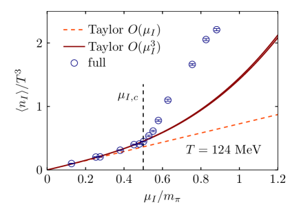
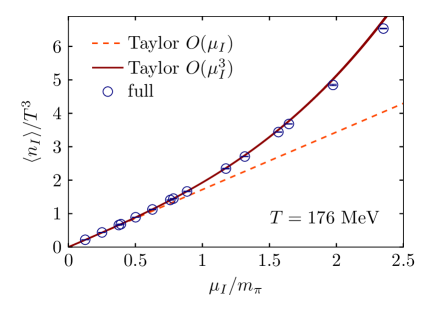
Figure 1: Results for $\left\langle n_{I}\right\rangle$ on $N_{t}=6$ lattices from direct simulations (blue points) in comparison to LO (orange dashed line) and NLO (red solid line) Taylor expansions for $T=124\textmd{ MeV}$ (top panel) and for $T=176$ MeV (bottom panel).

To perform a detailed comparison between the direct results for $\left\langle n_{I}\right\rangle$ and the Taylor expansion in a wide range of $\mu_{I}$, we have extended our existing results Brandt:2017oyy with new data up to $\mu_{I}\lesssim 325$ MeV. This value is still sufficiently far away from the saturation region for $N_{t}\geq 8$, ensuring that lattice artifacts remain under control (for all the results shown below, the chemical potential in lattice units satisfies $\mu_{I}a<0.3$). The comparison between the direct data for $\left\langle n_{I}\right\rangle$ and the results from the Taylor expansion is shown in Fig. 1 for $N_{t}=6$. For the lower temperature, $T=124$ MeV, the data reaches the BEC phase boundary at $\mu_{I,c}\approx m_{\pi}/2$. Up to this point the data shows remarkable agreement with both the LO and the NLO Taylor expansion. Slight differences between the data and the LO expansion become apparent close to $\mu_{I,c}$ (see also Fig. 7 in App. B at $T=113$ MeV). The lattice data starts to deviate from the Taylor expansion curve for $\mu_{I}>\mu_{I,c}$. This is certainly expected, since the Taylor expansion cannot capture the change of dynamics at the transition. In contrast, the results for $T=176$ MeV are above the BEC phase boundary. In this regime the agreement with Taylor expansion persists up to larger values of $\mu_{I}$ and starting at around $\mu_{I}/m_{\pi}\approx 0.6$ one can clearly see that the data favors NLO Taylor expansion over the LO expansion. Furthermore, Taylor expansion at NLO fails to describe $\left\langle n_{I}\right\rangle$ within the current uncertainties at around $\mu_{I}/m_{\pi}\approx 1.6$, where higher orders become important for this temperature.

Comparing the behavior of the data points between the two temperatures reveals another characteristic of the Taylor expansion. For low temperatures, the NLO expansion tends to underestimate the results for $\left\langle n_{I}\right\rangle$, while it overestimates them for higher temperatures. Due to continuity there will be a region, where the agreement between the NLO expansion and the full result is almost perfect. Outside the BEC phase, where the expansion converges to the correct result, this region is related to the suppression of higher order terms, most dominantly of $c_{6}(T)$, which is indeed expected to cross zero as $T$ increases. Inside the pion condensation phase this agreement is merely accidental and does not reveal any information about the interior of the BEC region.

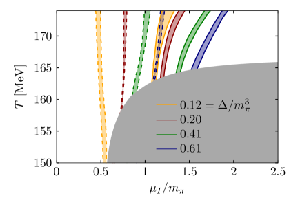
Figure 2: Contours of constant $\Delta^{\rm LO}$ (dashed bands) and $\Delta^{\rm NLO}$ (solid bands) for $N_{t}=8$. The shaded gray area indicates the BEC phase.

To quantify the regions in parameter space where Taylor expansion at a given order (LO or NLO) starts to become unreliable, we look at curves in parameter space with constant difference

$$\Delta^{\rm LO/NLO}=\big{|}\left\langle n_{I}\right\rangle-\left\langle n_{I}\right\rangle^{\rm LO/NLO}\big{|}$$ (3)

between the full results and the Taylor expansion. In the following we focus on the high temperature region, $T\gtrsim 150$ MeV, to be able to draw conclusions about the applicability range of the Taylor method in the absence of the BEC phase transition.

The contour lines are determined using a two-dimensional spline fit to $\Delta$, where the nodepoints have been generated via a Monte-Carlo analysis (for a description of our fit strategy, see Ref. Brandt:2016zdy ). In the spline fit we include the constraint that $\Delta=0$ for $\mu_{I}=0$. Note that we expect a rapid change of the data for $\Delta$ at the BEC phase boundary in the thermodynamic limit. For our finite volumes, for $T\gtrsim 150$ MeV the behavior is more regular and can be captured by a spline interpolation.

Our $N_{t}=8$ results for the contour lines are shown in Fig. 2 for various values of $\Delta$. The figure also includes the BEC phase boundary, which we extended to higher values of $\mu_{I}$ compared to Ref. Brandt:2017oyy , see App. C for details. Most of the contour lines have positive slopes, indicating the general tendency that the expansion performs better and better as the temperature increases. This is partly due to the fact that the actual dimensionless expansion parameter is $\mu_{I}/T$, cf. Eq. (2) – however, the contour lines differ from the simple $\mu/T=\textmd{const}.$ lines considerably (see below). The exception is the contour line with $\Delta^{\rm LO}/m_{\pi}^{3}=0.12$, which is roughly insensitive to the temperature. In addition, the results clearly reflect that the NLO expansion has a broader reliability range than the LO one, with contour lines shifted to considerably higher values of $\mu_{I}$.

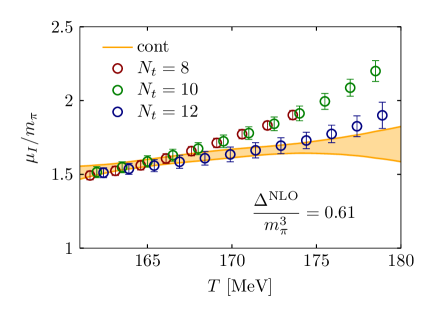
Figure 3: Continuum extrapolation for the contour line $\Delta^{\rm NLO}/m_{\pi}^{3}=0.61$. The yellow curve corresponds to the continuum extrapolation and the points show (every third of) the results from the individual lattices that were included in the fit. We have slightly shifted the data horizontally to enhance visibility.

Eventually we aim at investigating the range of applicability of the Taylor expansion in the continuum. To this end we perform a continuum extrapolation of the contour lines of $\Delta$, using a parameterization in terms of polynomials in $(T-T_{0})$ with lattice spacing dependent coefficients, setting $T_{0}=140$ MeV. In the continuum extrapolation we focus on $\Delta^{\rm NLO}$, for which the contours are well described by a second order polynomial for $T\geq 161$ MeV. In all of the cases the $N_{t}=6$ results were found to be outside of the scaling region and have thus been excluded from the fit. One of these extrapolations is visualized in Fig. 3 for $\Delta^{\rm NLO}/m_{\pi}^{3}=0.61$. Finally, the contour lines of $\Delta^{\rm NLO}$ in the continuum limit are plotted in Fig. 4, this time versus $\mu_{I}/T$. Once more, the gray area indicates the BEC phase in the continuum with the updated phase boundary from App. C. As discussed above, the naive expectation for the contours outside of the BEC phase are lines with $\mu/T=\textmd{const}.$, i.e. vertical lines in this plot. While this is approximately the case for large $\Delta^{\rm NLO}$, the contours with small values of $\Delta^{\rm NLO}$ show clear deviations from this expectation with the tendency to shift to larger values of $\mu_{I}/T$ with increasing temperature.

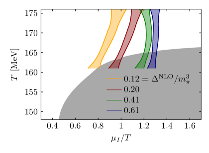
Figure 4: Continuum results for the contour lines of $\Delta^{\rm NLO}$. The gray shaded area indicates the BEC phase. Note that the curves stop at $T=161$ MeV, since only data above this temperature enters the continuum fit.

IV Testing the radius of convergence

As mentioned in the introduction, the radius of convergence of the Taylor expansion has been used extensively in the literature to extract information on the possible phase transitions of the theory for $\mu_{B}>0$. The current setup with $\mu_{I}>0$ is ideal to test the performance of this method in QCD, since the phase diagram features a second order phase transition Son:2000xc ; Brandt:2017oyy comparably close to the $\mu_{I}=0$ axis. We have already seen the breakdown of the expansion close to the phase boundary (cf. Fig. 1). We will now test whether the leading estimator for the radius of convergence also indicates the presence of this phase boundary.

A possible definition for the radius of convergence $r$ for the Taylor series of $\left\langle n_{I}\right\rangle$ from Eq. (2) is given by

$$r=\lim_{n\to\infty}r_{n}(n_{I}),\quad\frac{r_{n}(n_{I})}{T}=\sqrt{\frac{c_{n}}{c_{n+2}}(n+1)n}\,,$$ (4)

but note that for a general singularity in the complex $\mu_{I}$-plane this limit is not guaranteed to exist (see Ref. Vovchenko:2017gkg for a counter-example). Here $c_{n}$ are the coefficients of the expansion of the pressure defined in Sec. II. Note that while the same radius of convergence $r$ is encoded in the Taylor series of other observables, the estimators at finite $n$ can be quite different. In particular, comparing the series for the pressure $p$, the density $\left\langle n_{I}\right\rangle$ and the susceptibility $\left\langle\chi_{I}\right\rangle=\partial\left\langle n_{I}\right\rangle/\partial\mu_{I}$ gives

$$r_{n}(\chi_{I})=\sqrt{\frac{n-1}{n+1}}\,r_{n}(n_{I})=\sqrt{\frac{n(n-1)}{(n+2)(n+1)}}\,r_{n}(p)\,.$$ (5)

These indeed agree in the limit $n\to\infty$, but differ at finite $n$.

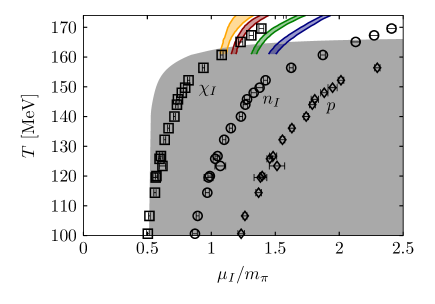
Figure 5: The leading-order estimators for the radius of convergence using the series for different observables on our $N_{t}=8$ ensembles. The results are compared to the boundary of the BEC phase (gray area) and to the contours of $\Delta^{\rm NLO}$ (colored bands).

With two coefficients at hand, only a single estimator can be constructed for $r$ and we cannot investigate the $n\to\infty$ limit systematically. The estimators for $r$ obtained from the different observables are shown in Fig. 5 for $N_{t}=8$. For comparison we also included the boundary of the BEC phase and the contour lines of $\Delta^{\rm NLO}$ in the figure. Both the estimators $r_{n}$ and the $n$-th order contour lines are expected to fall on top of the phase boundary in the limit $n\to\infty$ – as long as the BEC onset is the singularity closest to $\mu_{I}=0$.

The results for $r_{2}(\chi_{I})$ are observed to lie surprisingly close to the phase boundary for low temperatures, while $r_{2}(n_{I})$ and $r_{2}(p)$ significantly overestimate the radius of convergence. While such a perfect agreement for $r_{2}(\chi_{I})$ is likely accidental, similar tendencies were also found in an NJL-type model Karsch:2010hm , and in toy models of QCD with imaginary chemical potentials DElia:2016jqh , suggesting that the series of the susceptibility gives estimators with the fastest convergence rate. The estimators also reveal a considerable change of slope around $150-160\textmd{ MeV}$, close to the upper boundary of the BEC phase and in agreement with the qualitative trend that the two curves will agree in the limit $n\to\infty$. Finally, a qualitative agreement is also observed between the behavior of $r_{2}$ and the contours lines of $\Delta^{\rm NLO}$.

Up to now we have ignored a subtle issue regarding the estimators of the radius of convergence in finite volumes. In a finite volume $V$, phase transitions are smoothed out, but the partition function has Lee-Yang zeroes at complex $\mu_{I}$ that approach the real axis as $V\to\infty$ Yang:1952be , according to criticality Stephanov:2006dn . How this is connected to the $V$-dependence of the estimators $r_{n}$ is highly non-trivial. We find that the leading order Taylor coefficients depend only mildly on the volume. This is discussed in App. B together with the finite size effects of the full data.

V Conclusions

In this letter we have presented a detailed comparison between Taylor expansion and full simulations of QCD at nonzero isospin chemical potential $\mu_{I}$. This is a theory with a second-order phase transition between the normal phase and a phase with Bose-Einstein condensation of charged pions, enabling us to observe the breakdown of the Taylor expansion at the critical chemical potential. Up to the boundary of the BEC phase the full data for the isospin density $\left\langle n_{I}\right\rangle$ is well described by Taylor expansion – both by the leading- (LO) and the next-to-leading order (NLO) series.

To test the reliability of the expansion outside the BEC phase, we extended our lattice ensembles generated in Brandt:2017oyy with simulations at higher chemical potentials. The update for the BEC phase boundary up to $\mu_{I}\approx 325$ MeV is presented in App. C. To quantify the performance of the LO and NLO expansions in this region, we introduced the deviation $\Delta$ between the full and the Taylor-expanded results, see Eq. (3). The contour lines of $\Delta^{\rm LO}$ and $\Delta^{\rm NLO}$ are shown in Fig. 2 for our $N_{t}=8$ ensembles. Taking the $\Delta=0.2\,m_{\pi}^{3}$ contour (which corresponds to deviations of $3-6\%$ in the isospin density) as an indicator, the LO expansion is reliable up to $\mu_{I}/m_{\pi}\approx 0.5$ to $0.6$, while the NLO series performs reasonably well up to $\mu_{I}/m_{\pi}\approx 1.0$ to $1.5$. The continuum extrapolation of the contour lines is visualized in Fig. 4. Contrary to the naive expectation that the contours lie along lines of constant $\mu/T$ outside of the BEC phase, we find considerable deviations from this behavior, with a tendency towards larger values of $\mu/T$ with increasing temperature.

We have also compared the estimator $r_{2}$ for the radius of convergence, obtained from the first two coefficients ($c_{2}$ and $c_{4}$) of the Taylor expansion, to the critical chemical potential $\mu_{I,c}$ known from the full simulations. We find that both $r_{2}$ and $\mu_{I,c}$ change similarly with temperature, signaling the expected agreement when higher order estimates for the radius of convergence are taken into account. Concerning possible different definitions of $r$, we find that the estimate obtained from the susceptibility $\chi_{I}$ is closest to the phase boundary. Whether this remains true for higher-order estimators remains to be seen. Our findings demonstrate that already the leading estimators for the radius of convergence are sensitive to the phase transition. We emphasize, however, that a more detailed study including higher order estimates for $r$ is clearly desired and mandatory to be able to draw definite conclusions. Our study can be used to quantify the uncertainties of Taylor expansions in baryon chemical potentials and to guide the interpretation of results obtained for the radius of convergence of such series. This will also be of relevance for comparison to low energy models of QCD.

Acknowledgments The authors thank Szabolcs Borsányi for useful correspondence and for providing the data for the Taylor expansion coefficients, and Volodymyr Vovchenko for insightful comments. This research was funded by the DFG (Emmy Noether Programme EN 1064/2-1 and SFB/TRR 55). The simulations were performed on the GPU cluster of the Institute for Theoretical Physics at the University of Regensburg and on the FUCHS and LOEWE clusters at the Center for Scientific Computing of the Goethe University of Frankfurt.

Appendix A Computation and improved $\lambda$-extrapolations of $n_{I}$

In terms of the massless Dirac operator $\not{D}(\mu_{I})$ and the mass of the (degenerate) light quarks $m_{ud}$, the isospin density (1) is given by (cf. Ref. Brandt:2016zdy )

$$\left\langle n_{I}\right\rangle=\frac{T}{2V}\left\langle\textmd{Re }\textmd{tr}\,\frac{(\not{D}(\mu_{I})+m_{ud})^{\dagger}\partial_{\mu_{I}}\not{D}(\mu_{I})}{|\not{D}(\mu_{I})+m_{ud}|^{2}+\lambda^{2}}\right\rangle\,,$$ (6)

where $\partial_{\mu_{I}}$ is the derivative with respect to $\mu_{I}$. The trace in Eq. (6) can be evaluated using stochastic estimators, giving $n_{I}^{\rm stoch}$, or in the spectral representation

$$n_{I}=\frac{T}{2V}\sum_{n}\frac{\textmd{Re}\;\varphi_{n}^{\dagger}[\not{D}(\mu_{I})+m_{ud}]^{\dagger}\partial_{\mu_{I}}\not{D}(\mu_{I})\varphi_{n}}{\xi^{2}_{n}+\lambda^{2}}\,,$$ (7)

with the singular values $\xi_{n}$ and the associated eigenstates $\varphi_{n}$ (see Ref. Brandt:2017oyy for more details).

The spectral representation (7) is the basis for the improvement program introduced in Ref. Brandt:2017oyy . First we introduce the truncated difference

$$\begin{split}\delta^{N}&\equiv n_{I}^{N}(\lambda)-n_{I}^{N}(\lambda=0)\\ &\begin{split}=\frac{T}{2V}\sum_{n=1}^{N}&\textmd{Re}\;\varphi_{n}^{\dagger}[\not{D}(\mu_{I})+m_{ud}]^{\dagger}\partial_{\mu_{I}}\not{D}(\mu_{I})\varphi_{n}\\ &\times\left(\frac{1}{\xi_{n}^{2}+\lambda^{2}}-\frac{1}{\xi_{n}^{2}}\right)\,,\end{split}\end{split}$$ (8)

where $n_{I}^{N}(\lambda)$ is the operator from Eq. (7) with a singular value sum truncated at $n=N$. This truncated difference $\delta^{N}$ does not contribute in the $\lambda\to 0$ limit, allowing us to write

$$\lim_{\lambda\to 0}\left\langle n_{I}\right\rangle=\lim_{\lambda\to 0}\left\langle n_{I}^{\rm stoch}-\delta^{N}\right\rangle\,.$$ (9)

As indicated, the $\lambda>0$ value of the operator is determined using stochastic estimators, while the correction term $\delta^{N}$ is calculated in the spectral representation (8). In addition to the improvement of the operator, we also employ the leading order reweighting discussed in section III.4 of Ref. Brandt:2017oyy . This approximates the $\lambda=0$ distribution of the lattice ensembles and brings the expectation value $\left\langle n_{I}\right\rangle$ closer to its $\lambda=0$ limit.

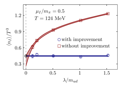
Figure 6: Improved $\lambda$-extrapolation for $\left\langle n_{I}\right\rangle$ on our $24^{3}\times 6$ ensemble in comparison to the unimproved one.

As discussed in Ref. Brandt:2017oyy , the optimal (or minimal) value of $N$ necessary to achieve sufficient improvement to obtain a controlled $\lambda$-extrapolation will in general depend on the operator. We find that the behavior of $n_{I}$ with $N$ is similar to the one of the chiral condensate, so that $N\approx 100$ is usually sufficient to obtain reasonably flat extrapolations. A particular example for the $\lambda$-extrapolations is provided in Fig. 6. The plot indicates the tremendous increase in reliability due to our improvement scheme, enabling a well controlled $\lambda$-extrapolation and precision results.

Appendix B Interpolation of Taylor expansion coefficients and finite size effects

The Taylor coefficients are combinations of derivatives of the pressure,

$$c_{n}=\left.\frac{\partial^{n}(p/T^{4})}{\partial(\mu_{I}/T)^{n}}\right|_{\mu_{I}=0}\,,\quad\quad\frac{p}{T^{4}}=\frac{1}{VT^{3}}\log\mathcal{Z}\,,$$ (10)

with respect to the isospin chemical potential at $\mu_{I}=0$. These can be rewritten using the quark chemical potentials $\mu_{u}$ and $\mu_{d}$ – in particular, $c_{2}$ and $c_{4}$ are given by

$$c_{2}=2\left.\Big{[}\partial_{u}^{2}\Big{(}\frac{p}{T^{4}}\Big{)}-\partial_{u}\partial_{d}\Big{(}\frac{p}{T^{4}}\Big{)}\Big{]}\right|_{\mu_{I}=0}$$ (11)

and

$$c_{4}=2\left.\Big{[}\partial_{u}^{4}\Big{(}\frac{p}{T^{4}}\Big{)}-4\partial_{u}^{3}\partial_{d}\Big{(}\frac{p}{T^{4}}\Big{)}+3\partial_{u}^{2}\partial_{d}^{2}\Big{(}\frac{p}{T^{4}}\Big{)}\Big{]}\right|_{\mu_{I}=0}\,,$$ (12)

where $\partial_{f}$ stands for the derivative with respect to $\mu_{f}/T$. The results for the coefficients $c_{2}$ and $c_{4}$ from Ref. Borsanyi:2011sw for the $24^{3}\times 8$ lattice are shown in the top panel of Fig. 7 together with a cubic spline interpolation.

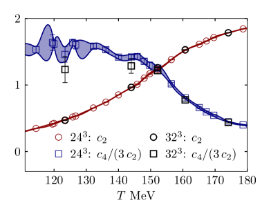
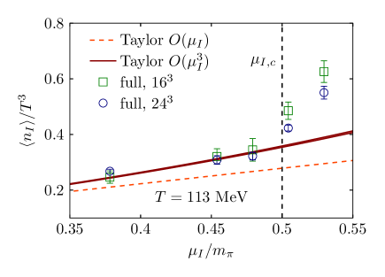
Figure 7: Top panel: Spline interpolation of the first two Taylor coefficients $c_{2}$ and $c_{4}$ (normalized by $3c_{2}$) on the $24^{3}\times 8$ lattices, compared to the results on the $32^{3}\times 8$ ensemble Borsanyi:2011sw . Bottom panel: Results for $\left\langle n_{I}\right\rangle$ on $N_{t}=6$ lattices from direct simulations with a spatial volume of $16^{3}$ (green boxes) and $24^{3}$ (blue circles) in comparison to LO (orange dashed line) and NLO (red solid line) Taylor expansions for $T=113\textmd{ MeV}$. The Taylor expansion coefficients have been obtained on a $18^{3}\times 6$ lattice Borsanyi:2011sw .

To check finite size effects in the temperature range of interest we also include the results from the $32^{3}\times 8$ ensemble from Ref. Borsanyi:2011sw in the top panel of Fig. 7. Apart from some visible but not significant effects for the $c_{4}$ coefficient at $T\lesssim 150$ MeV finite size effects are absent. To lend further support to the statement that finite size effects are negligible, we show the results for $\left\langle n_{I}\right\rangle$ obtained on $16^{3}\times 6$ and $24^{3}\times 6$ lattices in comparison to the Taylor expansion with coefficients from a $18^{3}\times 6$ lattice in the bottom panel of Fig. 7. For $\mu_{I}<\mu_{I,c}$, we see that the lattice results agree within uncertainties and are in mutual agreement with the NLO expansion. Also evident are the expected strong finite size effects at and just above $\mu_{I,c}$, outside the applicability region of the expansion.

The main part of our study has been done on $24^{3}\times 6$, $24^{3}\times 8$, $28^{3}\times 10$ and $36^{3}\times 12$ lattices. In contrast the Taylor coefficients have been computed on $18^{3}\times 6$, $24^{3}\times 8$, $32^{3}\times 8$, $32^{3}\times 10$ and $32^{3}\times 12$ lattices in Ref. Borsanyi:2011sw . Given the magnitude of finite size effects visible in Fig. 7, we can thus conclude that those effects are irrelevant within the present accuracy.

Appendix C The pion condensation phase boundary for large $\mu_{I}$

For the present study we extended the range of chemical potentials compared to Ref. Brandt:2017oyy , enabling a determination of the BEC phase boundary for higher values of $\mu_{I}$. We have performed new temperature scans in the range $120\textmd{ MeV}<\mu_{I}<325$ MeV, allowing to locate the critical temperature $T_{c}(\mu_{I})$, where the pion condensate vanishes. The results for three lattice spacings are shown in Fig. 8. Compared to our previous results Brandt:2017oyy we observe a slight increase in the critical temperature with all data points approximately lying along a constant line. To capture this behavior and to approach the continuum limit, we fit all points by the function $d_{1}+d_{2}/\mu_{I}^{2}$ with $a^{2}$-dependent coefficients $d_{1}$ and $d_{2}$. To smoothly connect to our previous result, the data of Brandt:2017oyy for $T<161\textmd{ MeV}$ and 90 MeV $\leq\mu_{I}\leq 120$ MeV for each value of $N_{t}$ and in the continuum are also included in the fit. The resulting continuum extrapolation is also shown in Fig. 8.

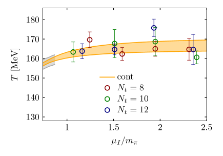
Figure 8: Continuum extrapolation (yellow band) of the BEC phase boundary based on results from three lattice ensembles (colored points). The gray band is the part of the continuum extrapolation from Ref. Brandt:2017oyy which enters the fit for the purpose of matching to the phase boundary for $\mu_{I}<120$ MeV.

References

- (1) P. de Forcrand, “Simulating QCD at finite density,” PoS LAT2009 (2009) 010, arXiv:1005.0539 [hep-lat].
- (2) G. Aarts, “Complex Langevin dynamics and other approaches at finite chemical potential,” PoS LATTICE2012 (2012) 017, arXiv:1302.3028 [hep-lat].
- (3) S. Gupta, “QCD at finite density,” PoS LATTICE2010 (2010) 007, arXiv:1101.0109 [hep-lat].
- (4) C. Gattringer, “New developments for dual methods in lattice field theory at non-zero density,” PoS LATTICE2013 (2014) 002, arXiv:1401.7788 [hep-lat].
- (5) H.-T. Ding, “Lattice QCD at nonzero temperature and density,” PoS LATTICE2016 (2017) 022, arXiv:1702.00151 [hep-lat].
- (6) S. A. Gottlieb, W. Liu, D. Toussaint, R. L. Renken, and R. L. Sugar, “Fermion Number Susceptibility in Lattice Gauge Theory,” Phys. Rev. D38 (1988) 2888–2896.
- (7) R. V. Gavai and S. Gupta, “Quark number susceptibilities, strangeness and dynamical confinement,” Phys. Rev. D64 (2001) 074506, arXiv:hep-lat/0103013 [hep-lat].
- (8) C. R. Allton, S. Ejiri, S. J. Hands, O. Kaczmarek, F. Karsch, E. Laermann, C. Schmidt, and L. Scorzato, “The QCD thermal phase transition in the presence of a small chemical potential,” Phys. Rev. D66 (2002) 074507, arXiv:hep-lat/0204010 [hep-lat].
- (9) A. Bazavov et al., “The QCD Equation of State to from Lattice QCD,” Phys. Rev. D95 no. 5, (2017) 054504, arXiv:1701.04325 [hep-lat].
- (10) S. Borsányi, Z. Fodor, J. N. Guenther, S. K. Katz, K. K. Szabó, A. Pásztor, I. Portillo, and C. Ratti, “Higher order fluctuations and correlations of conserved charges from lattice QCD,” arXiv:1805.04445 [hep-lat].
- (11) R. V. Gavai and S. Gupta, “The Critical end point of QCD,” Phys. Rev. D71 (2005) 114014, arXiv:hep-lat/0412035 [hep-lat].
- (12) C. R. Allton, M. Doring, S. Ejiri, S. J. Hands, O. Kaczmarek, F. Karsch, E. Laermann, and K. Redlich, “Thermodynamics of two flavor QCD to sixth order in quark chemical potential,” Phys. Rev. D71 (2005) 054508, arXiv:hep-lat/0501030 [hep-lat].
- (13) R. V. Gavai and S. Gupta, “QCD at finite chemical potential with six time slices,” Phys. Rev. D78 (2008) 114503, arXiv:0806.2233 [hep-lat].
- (14) M. D’Elia, G. Gagliardi, and F. Sanfilippo, “Higher order quark number fluctuations via imaginary chemical potentials in QCD,” Phys. Rev. D95 no. 9, (2017) 094503, arXiv:1611.08285 [hep-lat].
- (15) S. Datta, R. V. Gavai, and S. Gupta, “Quark number susceptibilities and equation of state at finite chemical potential in staggered QCD with Nt=8,” Phys. Rev. D95 no. 5, (2017) 054512, arXiv:1612.06673 [hep-lat].
- (16) S. Borsányi, Z. Fodor, S. D. Katz, S. Krieg, C. Ratti, and K. Szabó, “Fluctuations of conserved charges at finite temperature from lattice QCD,” JHEP 01 (2012) 138, arXiv:1112.4416 [hep-lat].
- (17) J. B. Kogut and D. K. Sinclair, “Quenched lattice QCD at finite isospin density and related theories,” Phys. Rev. D66 (2002) 014508, arXiv:hep-lat/0201017 [hep-lat].
- (18) J. B. Kogut and D. K. Sinclair, “Lattice QCD at finite isospin density at zero and finite temperature,” Phys. Rev. D66 (2002) 034505, arXiv:hep-lat/0202028 [hep-lat].
- (19) J. B. Kogut and D. K. Sinclair, “The Finite temperature transition for 2-flavor lattice QCD at finite isospin density,” Phys. Rev. D70 (2004) 094501, arXiv:hep-lat/0407027 [hep-lat].
- (20) P. de Forcrand, M. A. Stephanov, and U. Wenger, “On the phase diagram of QCD at finite isospin density,” PoS LAT2007 (2007) 237, arXiv:0711.0023 [hep-lat].
- (21) W. Detmold, K. Orginos, and Z. Shi, “Lattice QCD at non-zero isospin chemical potential,” Phys. Rev. D86 (2012) 054507, arXiv:1205.4224 [hep-lat].
- (22) P. Cea, L. Cosmai, M. D’Elia, A. Papa, and F. Sanfilippo, “The critical line of two-flavor QCD at finite isospin or baryon densities from imaginary chemical potentials,” Phys. Rev. D85 (2012) 094512, arXiv:1202.5700 [hep-lat].
- (23) G. Endrődi, “Magnetic structure of isospin-asymmetric QCD matter in neutron stars,” Phys. Rev. D90 no. 9, (2014) 094501, arXiv:1407.1216 [hep-lat].
- (24) B. B. Brandt, G. Endrődi, and S. Schmalzbauer, “QCD phase diagram for nonzero isospin-asymmetry,” Phys. Rev. D97 no. 5, (2018) 054514, arXiv:1712.08190 [hep-lat].
- (25) D. T. Son and M. A. Stephanov, “QCD at finite isospin density,” Phys. Rev. Lett. 86 (2001) 592–595, arXiv:hep-ph/0005225 [hep-ph].
- (26) S. Borsányi et al., “The QCD equation of state with dynamical quarks,” JHEP 11 (2010) 077, arXiv:1007.2580 [hep-lat].
- (27) B. B. Brandt and G. Endrődi, “QCD phase diagram with isospin chemical potential,” PoS LATTICE2016 (2016) 039, arXiv:1611.06758 [hep-lat].
- (28) V. Vovchenko, J. Steinheimer, O. Philipsen, and H. Stoecker, “Cluster Expansion Model for QCD Baryon Number Fluctuations: No Phase Transition at ,” Phys. Rev. D97 no. 11, (2018) 114030, arXiv:1711.01261 [hep-ph].
- (29) F. Karsch, B.-J. Schaefer, M. Wagner, and J. Wambach, “Towards finite density QCD with Taylor expansions,” Phys. Lett. B698 (2011) 256–264, arXiv:1009.5211 [hep-ph].
- (30) C.-N. Yang and T. D. Lee, “Statistical theory of equations of state and phase transitions. 1. Theory of condensation,” Phys. Rev. 87 (1952) 404–409.
- (31) M. A. Stephanov, “QCD critical point and complex chemical potential singularities,” Phys. Rev. D73 (2006) 094508, arXiv:hep-lat/0603014 [hep-lat].