Tensor Matched Kronecker-Structured Subspace Detection for Missing Information

Ishan Jindal, Student Member, IEEE and Matthew Nokleby, Member, IEEE
Department of Electrical and Computer Engineering, Wayne State University, Detroit, MI, 48202, USA
Email: {ishan.jindal, matthew.nokleby}@wayne.edu
Abstract

We consider the problem of detecting whether a tensor signal having many missing entities lies within a given low dimensional Kronecker-Structured (KS) subspace. This is a matched subspace detection problem. Tensor matched subspace detection problem is more challenging because of the intertwined signal dimensions. We solve this problem by projecting the signal onto the Kronecker structured subspace, which is a Kronecker product of different subspaces corresponding to each signal dimension. Under this framework, we define the KS subspaces and the orthogonal projection of signal onto the KS subspace. We prove that the reliable detection is possible as long as the cardinality of missing signal is greater than the dimensions of the KS subspace by bounding the residual energy of the sampling signal with high probability.

Index Terms:
Machine learning, subspace models, Kronecker-structured model, missing multi-dimensional signals.

I Introduction

The matched subspace detection problem arises in different scientific areas. This includes medical imaging such as in image representation [1], in shape detection [2], communication MIMO network systems [3, 4], matrix completion [5, 6] etc., where we need to detect whether a given signal lies within a subspace. The matched subspace detection is well studied problem [7, 8]. However, this problem become more challenging when the signal is not completely observable that is only a small subset of the signal entries are known and based on this observation we want to test whether a signal belongs to a given subspace.

To deal with subspace detection with missing information, [9] and [10] provides a way to deal with missing information in the signal. These available methods make an implicit assumption that the signal is present in vectorized form and convert a multi-dimensional signal into a single dimension before testing. Many real-world signals such as dynamic scene video [11] or tomographic images are inherently multi dimensional, which capture the spatial and temporal correlations within the data. However, by vectorizing the signal we lose the multi-dimensional structure of the data, which could be used to enhance the performance of the detector. Previous works, for example [12], consider general subspace structure, whereas our work applies a subspace model to tensors by supposing that each mode of the tensor lies approximately along a subspace similar to [13]. Equivalently, we preserve this multi-dimensional structure of the signal by projecting the signal onto Kronecker-structured subspace, which is a Kronecker product of a number of subspaces corresponding to the dimensionality of the signal, while observing only a small subset of the elements of the signal; hence the K-S subspace model is a special case of general subspace models. Authors in [14] and [15] show how the multi-dimensional structure in data can be well exploited for better classification and representation performance.

In this work, we present all our analysis for 2-D signals π˜βˆˆπ‘m1Γ—m2𝐘superscript𝐑subscriptπ‘š1subscriptπ‘š2{\mathbf{Y}}\in\mathbf{R}^{m_{1}\times m_{2}}. We study two different ways through which information can be missing, First, when the entire row and/or column of the 2-D signal is missing, represented by 𝐘Ωsubscript𝐘Ω{\mathbf{Y}}_{\Omega}. For instance, while capturing the EEG signals using number of electrodes placed over the scalp, one of the electrodes is broken or we miss to capture the signal for a time window. Second, a more general case, when only discrete entries are missing, that is, the missing entries need not to be in the form of entire rows and/or columns, represented by 𝐘Ω^subscript𝐘^Ξ©{\mathbf{Y}}_{\widehat{{\Omega}}}. We formulate a binary hypothesis test for the more general case of missing information, where given a Kronecker-structured subspace πƒβˆˆβ„m1​m2Γ—n1​n2𝐃superscriptℝsubscriptπ‘š1subscriptπ‘š2subscript𝑛1subscript𝑛2{\mathbf{D}}\in~{}\mathbb{R}^{m_{1}m_{2}\times n_{1}n_{2}} we need to find whether π˜βˆˆπƒπ˜πƒ{\mathbf{Y}}\in{\mathbf{D}} by just observing the samples of 𝐘𝐘{\mathbf{Y}} with or without noise.

We formulate the hypothesis test as β„‹0:π˜βˆˆπƒ:subscriptβ„‹0π˜πƒ\mathcal{H}_{0}:{\mathbf{Y}}\in{\mathbf{D}} and β„‹1:π˜βˆ‰πƒ:subscriptβ„‹1π˜πƒ\mathcal{H}_{1}:{\mathbf{Y}}\notin{\mathbf{D}}. This test follows immediately by computing the residual energy, that is, if π˜βˆˆπƒπ˜πƒ{\mathbf{Y}}\in{\mathbf{D}}, then the residual energy β€–π˜βˆ’π”Aβ€‹π˜π”Bβ€–F2=0superscriptsubscriptnorm𝐘superscript𝐔𝐴superscriptπ˜π”π΅πΉ20\left|\left|{\mathbf{Y}}-{\mathbf{U}}^{A}{\mathbf{Y}}{\mathbf{U}}^{B}\right|\right|_{F}^{2}=0 and β€–π˜Ξ©βˆ’π”Ξ©Aβ€‹π˜Ξ©β€‹π”Ξ©Bβ€–F2=0superscriptsubscriptnormsubscript𝐘Ωsuperscriptsubscript𝐔Ω𝐴subscript𝐘Ωsuperscriptsubscript𝐔Ω𝐡𝐹20\left|\left|{\mathbf{Y}}_{\Omega}-{\mathbf{U}}_{\Omega}^{A}{\mathbf{Y}}_{\Omega}{\mathbf{U}}_{\Omega}^{B}\right|\right|_{F}^{2}=0, where 𝐔Asuperscript𝐔𝐴{\mathbf{U}}^{A} and 𝐔Bsuperscript𝐔𝐡{\mathbf{U}}^{B} are the orthogonal projection operator onto row and column subspace, respectively. We show that the residual energies of the signal are bounded with high probability. The main result of this work answers, given the row and column subspaces with dimensions n1β‰ͺm1much-less-thansubscript𝑛1subscriptπ‘š1n_{1}\ll m_{1} and n2β‰ͺm2much-less-thansubscript𝑛2subscriptπ‘š2n_{2}\ll m_{2}, respectively, how many rows and columns of the 2-D signal must be observed in order to reliably detect whether the signal belongs to the given subspace.

The rest of the paper is organized as follows: In Section II, we define the Kronecker structured subspace model. We present the final results in Section III with the discussion and experiments in Section IV. The hypothesis testing for matched subspace detection is provided in Section V and finally, we conclude this work with future directions in Section VI.

Mathematical Notation: We use lowercase bold letters to represent vectors, such as 𝐱𝐱{\mathbf{x}} and use uppercase bold to represent matrices, such as 𝐘𝐘{\mathbf{Y}}. We use βŠ—tensor-product\otimes to represent the Kronecker product between two matrices.

II Model Definition

A two dimensional signal of interest π˜βˆˆβ„m1Γ—m2𝐘superscriptℝsubscriptπ‘š1subscriptπ‘š2{\mathbf{Y}}\in\,\mathbb{R}^{m_{1}\times m_{2}} is represented by a matrix π€βˆˆβ„m1Γ—n1𝐀superscriptℝsubscriptπ‘š1subscript𝑛1{\mathbf{A}}\in\mathbb{R}^{m_{1}\times n_{1}}, which describes the subspace on which the columns of 𝐘𝐘{\mathbf{Y}} approximately lie with n1≀m1subscript𝑛1subscriptπ‘š1n_{1}\leq m_{1}, and by πβˆˆβ„m2Γ—n2𝐁superscriptℝsubscriptπ‘š2subscript𝑛2{\mathbf{B}}\in\,\mathbb{R}^{m_{2}\times n_{2}}, which describes the subspace on which the rows of 𝐘𝐘{\mathbf{Y}} approximately lie with n2≀m2subscript𝑛2subscriptπ‘š2n_{2}\leq m_{2}, that is 𝐘=𝐀𝐗𝐁T𝐘superscript𝐀𝐗𝐁𝑇{\mathbf{Y}}={\mathbf{A}}{\mathbf{X}}{\mathbf{B}}^{T} where π—βˆˆβ„n1Γ—n2𝐗superscriptℝsubscript𝑛1subscript𝑛2{\mathbf{X}}\in\mathbb{R}^{n_{1}\times n_{2}} represents the coefficient matrix. We can also express 𝐘𝐘{\mathbf{Y}} in vectorized form

𝐲=(π€βŠ—π)​𝐱,𝐲tensor-product𝐀𝐁𝐱\mathbf{y}=({\mathbf{A}}\otimes{\mathbf{B}}){\mathbf{x}}, (1)

where 𝐲=vec​(𝐘)𝐲vec𝐘\mathbf{y}=\text{vec}({\mathbf{Y}}), 𝐱=vec​(𝐗)𝐱vec𝐗\mathbf{x}=\text{vec}({\mathbf{X}}) and βŠ—tensor-product\otimes denotes the Kronecker product. Similar to [9], we define the coherence of Kronecker-structured subspace  𝐃=π€βŠ—πβˆˆβ„m1​m2Γ—n1​n2𝐃tensor-product𝐀𝐁superscriptℝsubscriptπ‘š1subscriptπ‘š2subscript𝑛1subscript𝑛2{{\mathbf{D}}={\mathbf{A}}~{}\otimes{\mathbf{B}}~{}\in~{}\mathbb{R}^{m_{1}m_{2}\times n_{1}n_{2}}} as

μ​(𝐃):=m1​m2n1​n2​max𝑗​‖𝐔𝐃​ejA​Bβ€–22,assignπœ‡πƒsubscriptπ‘š1subscriptπ‘š2subscript𝑛1subscript𝑛2𝑗maxsubscriptsuperscriptnormsuperscript𝐔𝐃subscriptsuperscript𝑒𝐴𝐡𝑗22\displaystyle\mu({\mathbf{D}}):=\frac{m_{1}m_{2}}{n_{1}n_{2}}\underset{j}{\text{max}}\left|\left|{\mathbf{U}}^{{\mathbf{D}}}e^{AB}_{j}\right|\right|^{2}_{2}, (2)

where 𝐔D=𝐃​(𝐃T​𝐃)βˆ’1​𝐃Tsuperscript𝐔𝐷𝐃superscriptsuperscript𝐃𝑇𝐃1superscript𝐃𝑇{\mathbf{U}}^{D}={\mathbf{D}}\left({\mathbf{D}}^{T}{\mathbf{D}}\right)^{-1}{\mathbf{D}}^{T} is the orthogonal projection operator onto 𝐃𝐃{\mathbf{D}}, ejA​Bsuperscriptsubscript𝑒𝑗𝐴𝐡e_{j}^{AB} represents the standard basis vector and ||β‹…||2||\cdot||_{2} represents the euclidean norm of a vector. The coherence provides the amount of information we can expect from each sample to provide. From [5], the coherence can take values between Β 1≀μ​(𝐃)≀m1​m2n1​n21πœ‡πƒsubscriptπ‘š1subscriptπ‘š2subscript𝑛1subscript𝑛21\leq~{}\mu({\mathbf{D}})\leq\frac{m_{1}m_{2}}{n_{1}n_{2}}Β . For further analysis, we also need to know whether the signal has energy outside the n1subscript𝑛1n_{1} and n2subscript𝑛2n_{2} dimensional column and row subspaces, respectively. Therefore, we define the coherence of column and row subspaces as

μ​(𝐀)πœ‡π€\displaystyle\mu({\mathbf{A}}) :=m1n1​max𝑗​‖𝐔A​ejAβ€–22,assignabsentsubscriptπ‘š1subscript𝑛1𝑗maxsubscriptsuperscriptnormsuperscript𝐔𝐴subscriptsuperscript𝑒𝐴𝑗22\displaystyle:=\frac{m_{1}}{n_{1}}\underset{j}{\text{max}}\left|\left|{\mathbf{U}}^{A}e^{A}_{j}\right|\right|^{2}_{2}, (3)
μ​(𝐁)πœ‡π\displaystyle\mu({\mathbf{B}}) :=m2n2​max𝑗​‖𝐔B​ejBβ€–22.assignabsentsubscriptπ‘š2subscript𝑛2𝑗maxsubscriptsuperscriptnormsuperscript𝐔𝐡subscriptsuperscript𝑒𝐡𝑗22\displaystyle:=\frac{m_{2}}{n_{2}}\underset{j}{\text{max}}\left|\left|{\mathbf{U}}^{B}e^{B}_{j}\right|\right|^{2}_{2}. (4)

Where, 𝐔A=𝐀​(𝐀T​𝐀)βˆ’1​𝐀Tsuperscript𝐔𝐴𝐀superscriptsuperscript𝐀𝑇𝐀1superscript𝐀𝑇{\mathbf{U}}^{A}={\mathbf{A}}\left({\mathbf{A}}^{T}{\mathbf{A}}\right)^{-1}{\mathbf{A}}^{T} and 𝐔B=𝐁​(𝐁T​𝐁)βˆ’1​𝐁Tsuperscript𝐔𝐡𝐁superscriptsuperscript𝐁𝑇𝐁1superscript𝐁𝑇{\mathbf{U}}^{B}={\mathbf{B}}\left({\mathbf{B}}^{T}{\mathbf{B}}\right)^{-1}{\mathbf{B}}^{T} are the projection operators onto 𝐀𝐀{\mathbf{A}} and 𝐁𝐁{\mathbf{B}} subspace, respectively and can take values Β 1≀μ​(𝐀)≀m1n11πœ‡π€subscriptπ‘š1subscript𝑛11\leq~{}\mu({\mathbf{A}})\leq\frac{m_{1}}{n_{1}}Β  and Β 1≀μ​(𝐁)≀m2n21πœ‡πsubscriptπ‘š2subscript𝑛21\leq~{}\mu({\mathbf{B}})\leq\frac{m_{2}}{n_{2}}Β . To establish the relationship between the coherence of Kronecker-structured subspace with the coherence of individual subspaces we need the Lemma 5.

Lemma 1.

The coherence of the Kronecker-structured subspace is equal to the product of coherence of individual subspaces, that is

μ​(π€βŠ—π)=μ​(𝐀)​μ​(𝐁).πœ‡tensor-productπ€ππœ‡π€πœ‡π\mu({\mathbf{A}}\otimes{\mathbf{B}})=\mu({\mathbf{A}})\mu({\mathbf{B}}). (5)
Proof.

in Appendix B ∎

μ​(𝐀)πœ‡π€\mu({\mathbf{A}}) achieves minimum values when all the vectors whose all the entries have magnitude 1n11subscript𝑛1\frac{1}{\sqrt{n_{1}}} forms 𝐀𝐀{\mathbf{A}} and if 𝐀𝐀{\mathbf{A}} contains a standard basis element then μ​(𝐀)πœ‡π€\mu({\mathbf{A}}) achieves the maximum value m1n1subscriptπ‘š1subscript𝑛1\frac{m_{1}}{n_{1}}. Similar analysis holds for μ​(𝐁)πœ‡π\mu({\mathbf{B}}) and μ​(𝐃)πœ‡πƒ\mu({\mathbf{D}}). For a 2-D signal 𝐘𝐘{\mathbf{Y}}, we let μ​(𝐘)πœ‡π˜\mu({\mathbf{Y}}) defines the coherence of the subspace spanned by the signal 𝐘𝐘{\mathbf{Y}} and we define the l∞subscript𝑙l_{\infty} norm as β€–π˜β€–βˆž=maxi,j​abs​(π˜β€‹(i,j))subscriptnormπ˜π‘–π‘—absπ˜π‘–π‘—||{\mathbf{Y}}||_{\infty}=\underset{{i,j}}{\max}\,\,\text{abs}({\mathbf{Y}}(i,j)). From [5], we write μ​(𝐘)=m1​m2β€‹β€–π˜β€–βˆž2|Y||F2πœ‡π˜subscriptπ‘š1subscriptπ‘š2superscriptsubscriptnorm𝐘2evaluated-atπ‘ŒπΉ2\mu({\mathbf{Y}})=m_{1}m_{2}\frac{||{\mathbf{Y}}||_{\infty}^{2}}{|\\ Y||_{F}^{2}}.

II-A Missing Signals

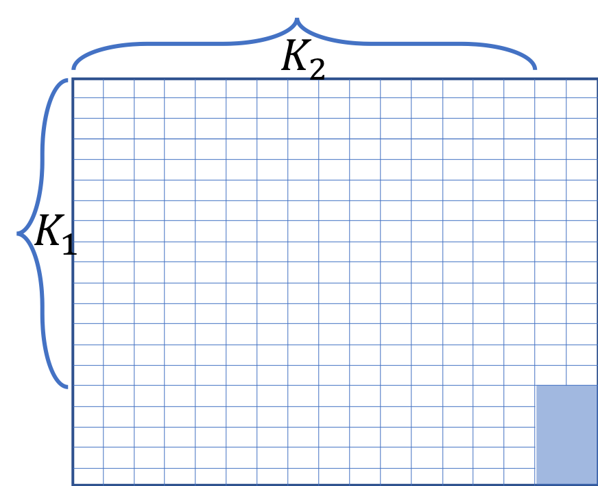
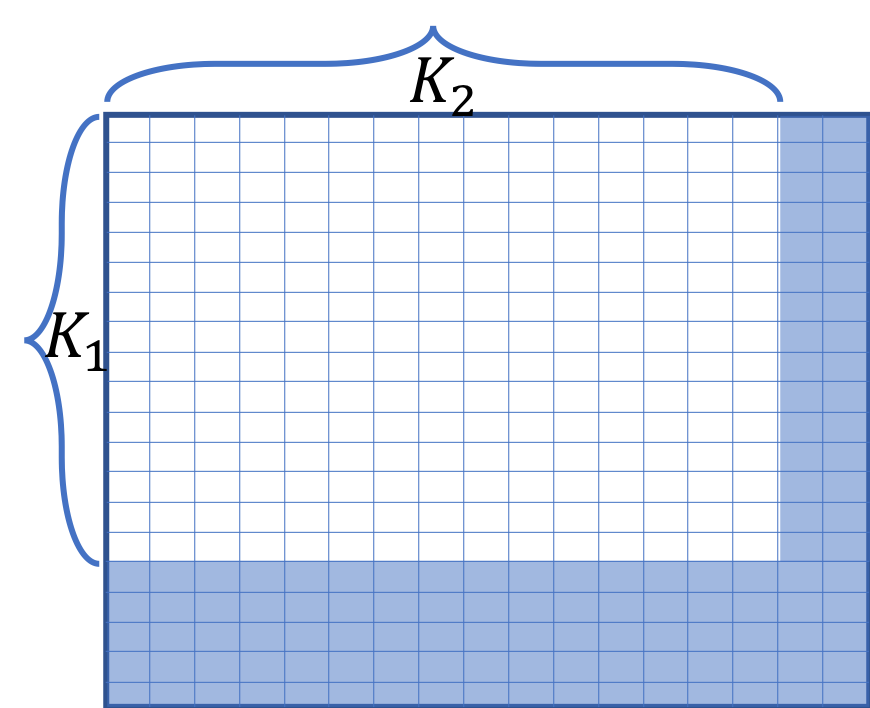
For tensor signals, we can expect signal entries to be missing along one or many dimensions, for instance, in Fig. 1(a) entire rows and columns of the 2-D signal 𝐘𝐘{\mathbf{Y}} are missing. We represent the signal with this type of missing information as 𝐘Ωsubscript𝐘Ω{\mathbf{Y}}_{\Omega}, where Ξ©k1​k2subscriptΞ©subscriptπ‘˜1subscriptπ‘˜2\Omega_{k_{1}k_{2}} represents the index of non-zero rows (k1)subscriptπ‘˜1(k_{1}) and non-zeros columns (k2)subscriptπ‘˜2(k_{2}). Now onwards, we use shorthand ΩΩ\Omega in replace of Ξ©k1​k2subscriptΞ©subscriptπ‘˜1subscriptπ‘˜2\Omega_{k_{1}k_{2}} throughout the paper. Thus, 𝐘Ωsubscript𝐘Ω{\mathbf{Y}}_{\Omega} is a signal of dimension k1Γ—k2subscriptπ‘˜1subscriptπ‘˜2k_{1}\times k_{2}. The energy of the signal 𝐘𝐘{\mathbf{Y}} in the subspace π€βŠ—πtensor-product𝐀𝐁{\mathbf{A}}\otimes{\mathbf{B}} is ‖𝐔Aβ€‹π˜β€‹(𝐔B)Tβ€–F2superscriptsubscriptnormsuperscriptπ”π΄π˜superscriptsuperscript𝐔𝐡𝑇𝐹2\left|\left|{\mathbf{U}}^{A}{\mathbf{Y}}({\mathbf{U}}^{B})^{T}\right|\right|_{F}^{2}, where 𝐔Asuperscript𝐔𝐴{\mathbf{U}}^{A} and 𝐔Bsuperscript𝐔𝐡{\mathbf{U}}^{B} are the column and row projection operator onto 𝐀𝐀{\mathbf{A}} and 𝐁𝐁{\mathbf{B}} subspaces, respectively and ||β‹…||F||\cdot||_{F} represents the Frobenius norm of the matrix.

Now, we define the column and row subspace for missing signal as π€Ξ©βˆˆπ‘k1Γ—n1subscript𝐀Ωsuperscript𝐑subscriptπ‘˜1subscript𝑛1{\mathbf{A}}_{\Omega}\in\mathbf{R}^{k_{1}\times n_{1}} and πΞ©βˆˆπ‘k2Γ—n2subscript𝐁Ωsuperscript𝐑subscriptπ‘˜2subscript𝑛2{\mathbf{B}}_{\Omega}\in\mathbf{R}^{k_{2}\times n_{2}}. Here, k1subscriptπ‘˜1k_{1} and k2subscriptπ‘˜2k_{2} are the columns and rows of 𝐀𝐀{\mathbf{A}} and 𝐁𝐁{\mathbf{B}}, respectively indexed by the set Ξ©k1​k2subscriptΞ©subscriptπ‘˜1subscriptπ‘˜2\Omega_{k_{1}k_{2}}, arranged in lexigraphic order. Since we only observe the signal 𝐘𝐘{\mathbf{Y}} for the set of rows and columns indexed by Ξ©k1​k2subscriptΞ©subscriptπ‘˜1subscriptπ‘˜2\Omega_{k_{1}k_{2}}, we estimate the missing signal energy 𝐘Ωsubscript𝐘Ω{\mathbf{Y}}_{\Omega} in 𝐃𝐃{\mathbf{D}} as how well the missing signal is best represented by the subspace 𝐃Ω=π€Ξ©βŠ—πΞ©subscript𝐃Ωtensor-productsubscript𝐀Ωsubscript𝐁Ω{\mathbf{D}}_{\Omega}={\mathbf{A}}_{\Omega}\otimes{\mathbf{B}}_{\Omega} with the projection operator 𝐔ΩD=𝐃Ω​(𝐃ΩT​𝐃Ω)βˆ’1​𝐃ΩTsuperscriptsubscript𝐔Ω𝐷subscript𝐃Ωsuperscriptsuperscriptsubscript𝐃Ω𝑇subscript𝐃Ω1superscriptsubscript𝐃Ω𝑇{\mathbf{U}}_{\Omega}^{D}={\mathbf{D}}_{\Omega}\left({\mathbf{D}}_{\Omega}^{T}{\mathbf{D}}_{\Omega}\right)^{-1}{\mathbf{D}}_{\Omega}^{T}. Therefore, if the row and columns of signal 𝐘𝐘{\mathbf{Y}} lies in row and column subspace then β€–π˜βˆ’π”Aβ€‹π˜π”Bβ€–F2=0superscriptsubscriptnorm𝐘superscript𝐔𝐴superscriptπ˜π”π΅πΉ20\left|\left|{\mathbf{Y}}-{\mathbf{U}}^{A}{\mathbf{Y}}{\mathbf{U}}^{B}\right|\right|_{F}^{2}=0 and hence

β€–π˜Ξ©βˆ’π”Ξ©Aβ€‹π˜Ξ©β€‹π”Ξ©Bβ€–F2=β€–π˜Ξ©βˆ’π˜^Ξ©β€–F2=0,superscriptsubscriptnormsubscript𝐘Ωsuperscriptsubscript𝐔Ω𝐴subscript𝐘Ωsuperscriptsubscript𝐔Ω𝐡𝐹2superscriptsubscriptnormsubscript𝐘Ωsubscript^𝐘Ω𝐹20\left|\left|{\mathbf{Y}}_{\Omega}-{\mathbf{U}}_{\Omega}^{A}{\mathbf{Y}}_{\Omega}{\mathbf{U}}_{\Omega}^{B}\right|\right|_{F}^{2}=\left|\left|{\mathbf{Y}}_{\Omega}-\widehat{{\mathbf{Y}}}_{\Omega}\right|\right|_{F}^{2}=0,

where 𝐔ΩA=𝐀Ω​(𝐀ΩT​𝐀Ω)βˆ’1​𝐀ΩTsuperscriptsubscript𝐔Ω𝐴subscript𝐀Ωsuperscriptsuperscriptsubscript𝐀Ω𝑇subscript𝐀Ω1superscriptsubscript𝐀Ω𝑇{\mathbf{U}}_{\Omega}^{A}={\mathbf{A}}_{\Omega}\left({\mathbf{A}}_{\Omega}^{T}{\mathbf{A}}_{\Omega}\right)^{-1}{\mathbf{A}}_{\Omega}^{T} and 𝐔ΩB=𝐁Ω​(𝐁ΩT​𝐁Ω)βˆ’1​𝐁ΩTsuperscriptsubscript𝐔Ω𝐡subscript𝐁Ωsuperscriptsuperscriptsubscript𝐁Ω𝑇subscript𝐁Ω1superscriptsubscript𝐁Ω𝑇{\mathbf{U}}_{\Omega}^{B}={\mathbf{B}}_{\Omega}\left({\mathbf{B}}_{\Omega}^{T}{\mathbf{B}}_{\Omega}\right)^{-1}{\mathbf{B}}_{\Omega}^{T}.

However, it is not always true that the entire row or/and entire column of the signal is missing. It may be the case that, while collecting the sensor output, some sensors are dead for a period of time and then wake up again. Therefore, we extend our analysis to a more general case of missing information, that is when any particular entry in the signal is missing as shown in Fig. 1(b) where only a fraction of entries are missing. We represent the signal with missing discrete entries as 𝐘Ω^​(k1,k2)subscript𝐘^Ξ©subscriptπ‘˜1subscriptπ‘˜2{\mathbf{Y}}_{\widehat{{\Omega}}(k_{1},k_{2})}, where Ξ©^​(k1,k2)={(i,j)β€‹βˆ€(i,j)|𝐘Ω^​(i,j)β‰ 0}^Ξ©subscriptπ‘˜1subscriptπ‘˜2conditional-set𝑖𝑗for-all𝑖𝑗subscript𝐘^Ω𝑖𝑗0\widehat{\Omega}(k_{1},k_{2})=\{(i,j)\forall(i,j)|{\mathbf{Y}}_{\widehat{{\Omega}}(i,j)}\neq 0\} represents the location of all the non-zero entries.

When the entire rows and/or columns of the signal are missing, we represent the remaining signal as the intersection of remaining rows and columns. Whereas, when discrete entries are missing, we represent the remaining signal as the signal minus the intersection of rows and/or columns that contains missing entries, we call it as union of dimensions. For further clarification, in Fig. 1 we plot a 2-D signal π˜βˆˆπ‘20Γ—17𝐘superscript𝐑2017{\mathbf{Y}}\in\mathbf{R}^{20\times 17} with m1=20subscriptπ‘š120m_{1}=20 and m2=17subscriptπ‘š217m_{2}=17. Let 5 rows and 2 columns of the signal 𝐘𝐘{\mathbf{Y}} is missing, we represent the remaining signal as the intersection of k1=m1βˆ’5=15subscriptπ‘˜1subscriptπ‘š1515k_{1}=m_{1}-5=15 and k2=m2βˆ’2=15subscriptπ‘˜2subscriptπ‘š2215k_{2}=m_{2}-2=15 in Fig. 1(a). Similarly, for the missing discrete entries we count the number of rows and columns to which the missing entries belongs and subtract the count from corresponding signal dimensions to obtain k1subscriptπ‘˜1k_{1} and k2subscriptπ‘˜2k_{2}. Finally subtract the intersection of the k1subscriptπ‘˜1k_{1} and k2subscriptπ‘˜2k_{2} from the signal to represent the remaining signal as shown in Fig. 1(b).
Refer to caption
(a) 𝐘Ωk1​k2subscript𝐘subscriptΞ©subscriptπ‘˜1subscriptπ‘˜2{\mathbf{Y}}_{\Omega_{k_{1}k_{2}}}
Refer to caption
(b) 𝐘Ω^​(k1,k2)subscript𝐘^Ξ©subscriptπ‘˜1subscriptπ‘˜2{\mathbf{Y}}_{\widehat{{\Omega}}(k_{1},k_{2})}
Figure 1: (a) Intersection and (b) union of rows and columns.

III Main Results

Theorem 1.

Let the entire rows or/and columns of the signal be missing, Ξ΄>0𝛿0\delta>0, k1β‰₯83​n1​μ​(𝐀)​log⁑(2​n1Ξ΄)subscriptπ‘˜183subscript𝑛1πœ‡π€2subscript𝑛1𝛿k_{1}\geq\frac{8}{3}n_{1}\mu({\mathbf{A}})\log\left(\frac{2n_{1}}{\delta}\right) and k2β‰₯83​n2​μ​(𝐁)​log⁑(2​n2Ξ΄)subscriptπ‘˜283subscript𝑛2πœ‡π2subscript𝑛2𝛿k_{2}\geq\frac{8}{3}n_{2}\mu({\mathbf{B}})\log\left(\frac{2n_{2}}{\delta}\right), than with probability at least 1βˆ’8​δ18𝛿1-8\delta,

((1βˆ’Ξ±)​(k1​k2m1​m2)βˆ’(Ξ²+1)22​(1βˆ’Ξ³2)​(1βˆ’Ξ³1)​(n1m1​μ​(𝐀)+n2m2​μ​(𝐁)))β€‹β€–π˜βˆ’π”Aβ€‹π˜π”Bβ€–F2β‰€β€–π˜Ξ©βˆ’π”Ξ©Aβ€‹π˜Ξ©β€‹π”Ξ©Bβ€–F2≀(1+Ξ±)​(k1​k2m1​m2)β€‹β€–π˜βˆ’π”Aβ€‹π˜π”Bβ€–F2,1𝛼subscriptπ‘˜1subscriptπ‘˜2subscriptπ‘š1subscriptπ‘š2superscript𝛽1221subscript𝛾21subscript𝛾1subscript𝑛1subscriptπ‘š1πœ‡π€subscript𝑛2subscriptπ‘š2πœ‡πsubscriptsuperscriptnorm𝐘superscript𝐔𝐴superscriptπ˜π”π΅2𝐹superscriptsubscriptnormsubscript𝐘Ωsubscriptsuperscript𝐔𝐴Ωsubscript𝐘Ωsubscriptsuperscript𝐔𝐡Ω𝐹21𝛼subscriptπ‘˜1subscriptπ‘˜2subscriptπ‘š1subscriptπ‘š2superscriptsubscriptnorm𝐘superscript𝐔𝐴superscriptπ˜π”π΅πΉ2\Bigg{(}(1-\alpha)\left(\frac{k_{1}k_{2}}{m_{1}m_{2}}\right)-\frac{(\beta+1)^{2}}{2(1-\gamma_{2})(1-\gamma_{1})}\Big{(}\frac{n_{1}}{m_{1}}\mu({\mathbf{A}})+\frac{n_{2}}{m_{2}}\mu({\mathbf{B}})\Big{)}\Bigg{)}||{\mathbf{Y}}-{\mathbf{U}}^{A}{\mathbf{Y}}{\mathbf{U}}^{B}||^{2}_{F}\leq||{\mathbf{Y}}_{\Omega}-{\mathbf{U}}^{A}_{\Omega}{\mathbf{Y}}_{\Omega}{\mathbf{U}}^{B}_{\Omega}||_{F}^{2}\\ \leq(1+\alpha)\left(\frac{k_{1}k_{2}}{m_{1}m_{2}}\right)\left|\left|{\mathbf{Y}}-{\mathbf{U}}^{A}{\mathbf{Y}}{\mathbf{U}}^{B}\right|\right|_{F}^{2}, (6)

where Ξ±=2​μ​(𝐘)2k1​k2​log⁑(1Ξ΄)𝛼2πœ‡superscript𝐘2subscriptπ‘˜1subscriptπ‘˜21𝛿\alpha=\sqrt{\frac{2\mu({\mathbf{Y}})^{2}}{k_{1}k_{2}}\log(\frac{1}{\delta})}, Ξ²=4​μ​(𝐘)​log⁑(1Ξ΄)(m2n2​1μ​(𝐁)+m1n2​1μ​(𝐀))𝛽4πœ‡π˜1𝛿subscriptπ‘š2subscript𝑛21πœ‡πsubscriptπ‘š1subscript𝑛21πœ‡π€\beta=\sqrt{\frac{4\mu({\mathbf{Y}})\log(\frac{1}{\delta})}{\left(\frac{m_{2}}{n_{2}}\frac{1}{\mu({\mathbf{B}})}+\frac{m_{1}}{n_{2}}\frac{1}{\mu({\mathbf{A}})}\right)}}, Ξ³1=8​n1​μ​(𝐀)3​k1​log⁑(2​n1Ξ΄)subscript𝛾18subscript𝑛1πœ‡π€3subscriptπ‘˜12subscript𝑛1𝛿\gamma_{1}=\sqrt{\frac{8n_{1}\mu({\mathbf{A}})}{3k_{1}}\log\left(\frac{2n_{1}}{\delta}\right)} and Ξ³2=8​n2​μ​(𝐀)3​k2​log⁑(2​n2Ξ΄)subscript𝛾28subscript𝑛2πœ‡π€3subscriptπ‘˜22subscript𝑛2𝛿\gamma_{2}=\sqrt{\frac{8n_{2}\mu({\mathbf{A}})}{3k_{2}}\log\left(\frac{2n_{2}}{\delta}\right)}.

Proof.

To prove this theorem, we first solve for the residual energy as follows

β€–π˜Ξ©βˆ’π”Ξ©Aβ€‹π˜Ξ©β€‹π”Ξ©Bβ€–F2superscriptsubscriptnormsubscript𝐘Ωsubscriptsuperscript𝐔𝐴Ωsubscript𝐘Ωsubscriptsuperscript𝐔𝐡Ω𝐹2\displaystyle||{\mathbf{Y}}_{\Omega}-{\mathbf{U}}^{A}_{\Omega}{\mathbf{Y}}_{\Omega}{\mathbf{U}}^{B}_{\Omega}||_{F}^{2} =tr​((π˜Ξ©βˆ’π”Ξ©Aβ€‹π˜Ξ©β€‹π”Ξ©B)T​(π˜Ξ©βˆ’π”Ξ©Aβ€‹π˜Ξ©β€‹π”Ξ©B))absenttrsuperscriptsubscript𝐘Ωsubscriptsuperscript𝐔𝐴Ωsubscript𝐘Ωsubscriptsuperscript𝐔𝐡Ω𝑇subscript𝐘Ωsubscriptsuperscript𝐔𝐴Ωsubscript𝐘Ωsubscriptsuperscript𝐔𝐡Ω\displaystyle=\text{tr}\left(\left({\mathbf{Y}}_{\Omega}-{\mathbf{U}}^{A}_{\Omega}{\mathbf{Y}}_{\Omega}{\mathbf{U}}^{B}_{\Omega}\right)^{T}\left({\mathbf{Y}}_{\Omega}-{\mathbf{U}}^{A}_{\Omega}{\mathbf{Y}}_{\Omega}{\mathbf{U}}^{B}_{\Omega}\right)\right)
=β€–π˜Ξ©β€–F2βˆ’tr​(𝐘ΩT​𝐔ΩAβ€‹π˜Ξ©β€‹π”Ξ©B)absentsuperscriptsubscriptnormsubscript𝐘Ω𝐹2trsuperscriptsubscriptπ˜Ξ©π‘‡subscriptsuperscript𝐔𝐴Ωsubscript𝐘Ωsubscriptsuperscript𝐔𝐡Ω\displaystyle=\left|\left|{\mathbf{Y}}_{\Omega}\right|\right|_{F}^{2}-\text{tr}\left({\mathbf{Y}}_{\Omega}^{T}{\mathbf{U}}^{A}_{\Omega}{\mathbf{Y}}_{\Omega}{\mathbf{U}}^{B}_{\Omega}\right)
=β€–π˜Ξ©β€–F2βˆ’tr​(𝐘ΩT​𝐀Ω​(𝐀ΩT​𝐀Ω)βˆ’1​𝐀ΩTβ€‹π˜Ξ©β€‹πΞ©β€‹(𝐁ΩT​𝐁Ω)βˆ’1​𝐁ΩT).absentsuperscriptsubscriptnormsubscript𝐘Ω𝐹2trsuperscriptsubscriptπ˜Ξ©π‘‡subscript𝐀Ωsuperscriptsuperscriptsubscript𝐀Ω𝑇subscript𝐀Ω1superscriptsubscript𝐀Ω𝑇subscript𝐘Ωsubscript𝐁Ωsuperscriptsuperscriptsubscript𝐁Ω𝑇subscript𝐁Ω1superscriptsubscript𝐁Ω𝑇\displaystyle=\left|\left|{\mathbf{Y}}_{\Omega}\right|\right|_{F}^{2}-\text{tr}\left({\mathbf{Y}}_{\Omega}^{T}{\mathbf{A}}_{\Omega}\left({\mathbf{A}}_{\Omega}^{T}{\mathbf{A}}_{\Omega}\right)^{-1}{\mathbf{A}}_{\Omega}^{T}{\mathbf{Y}}_{\Omega}{\mathbf{B}}_{\Omega}\left({\mathbf{B}}_{\Omega}^{T}{\mathbf{B}}_{\Omega}\right)^{-1}{\mathbf{B}}_{\Omega}^{T}\right). (7)

Now to solve the second part in (7), define 𝐓ΩT​𝐓Ω=(𝐀ΩT​𝐀Ω)βˆ’1superscriptsubscript𝐓Ω𝑇subscript𝐓Ωsuperscriptsuperscriptsubscript𝐀Ω𝑇subscript𝐀Ω1\mathbf{T}_{\Omega}^{T}\mathbf{T}_{\Omega}=\left({\mathbf{A}}_{\Omega}^{T}{\mathbf{A}}_{\Omega}\right)^{-1} and 𝐕Ω​𝐕ΩT=(𝐁ΩT​𝐁Ω)βˆ’1subscript𝐕Ωsuperscriptsubscript𝐕Ω𝑇superscriptsuperscriptsubscript𝐁Ω𝑇subscript𝐁Ω1\mathbf{V}_{\Omega}\mathbf{V}_{\Omega}^{T}=\left({\mathbf{B}}_{\Omega}^{T}{\mathbf{B}}_{\Omega}\right)^{-1}. Using the rotation property of trace we write

tr​(𝐘ΩT​𝐀Ω​𝐓ΩT​𝐓Ω​𝐀ΩTβ€‹π˜Ξ©β€‹πΞ©β€‹π•Ξ©β€‹π•Ξ©T​𝐁ΩT)=‖𝐓Ω​𝐀ΩTβ€‹π˜Ξ©β€‹πΞ©β€‹π•Ξ©Tβ€–F2.trsuperscriptsubscriptπ˜Ξ©π‘‡subscript𝐀Ωsuperscriptsubscript𝐓Ω𝑇subscript𝐓Ωsuperscriptsubscript𝐀Ω𝑇subscript𝐘Ωsubscript𝐁Ωsubscript𝐕Ωsuperscriptsubscript𝐕Ω𝑇superscriptsubscript𝐁Ω𝑇superscriptsubscriptnormsubscript𝐓Ωsuperscriptsubscript𝐀Ω𝑇subscript𝐘Ωsubscript𝐁Ωsuperscriptsubscript𝐕Ω𝑇𝐹2\text{tr}\left({\mathbf{Y}}_{\Omega}^{T}{\mathbf{A}}_{\Omega}\mathbf{T}_{\Omega}^{T}\mathbf{T}_{\Omega}{\mathbf{A}}_{\Omega}^{T}{\mathbf{Y}}_{\Omega}{\mathbf{B}}_{\Omega}\mathbf{V}_{\Omega}\mathbf{V}_{\Omega}^{T}{\mathbf{B}}_{\Omega}^{T}\right)\\ =\left|\left|\mathbf{T}_{\Omega}{\mathbf{A}}_{\Omega}^{T}{\mathbf{Y}}_{\Omega}{\mathbf{B}}_{\Omega}\mathbf{V}_{\Omega}^{T}\right|\right|_{F}^{2}. (8)

Substituting 𝐓ΩT​𝐓Ωsuperscriptsubscript𝐓Ω𝑇subscript𝐓Ω\mathbf{T}_{\Omega}^{T}\mathbf{T}_{\Omega} and 𝐕Ω​𝐕ΩTsubscript𝐕Ωsuperscriptsubscript𝐕Ω𝑇\mathbf{V}_{\Omega}\mathbf{V}_{\Omega}^{T} we obtain (7) as:

β€–π˜Ξ©βˆ’π˜^Ξ©β€–F2superscriptsubscriptnormsubscript𝐘Ωsubscript^𝐘Ω𝐹2\displaystyle\left|\left|{\mathbf{Y}}_{\Omega}-\widehat{{\mathbf{Y}}}_{\Omega}\right|\right|_{F}^{2} =β€–π˜Ξ©β€–F2βˆ’β€–π“Ξ©β€‹π€Ξ©Tβ€‹π˜Ξ©β€‹πΞ©β€‹π•Ξ©Tβ€–F2absentsuperscriptsubscriptnormsubscript𝐘Ω𝐹2superscriptsubscriptnormsubscript𝐓Ωsuperscriptsubscript𝐀Ω𝑇subscript𝐘Ωsubscript𝐁Ωsuperscriptsubscript𝐕Ω𝑇𝐹2\displaystyle=\left|\left|{\mathbf{Y}}_{\Omega}\right|\right|_{F}^{2}-\left|\left|\mathbf{T}_{\Omega}{\mathbf{A}}_{\Omega}^{T}{\mathbf{Y}}_{\Omega}{\mathbf{B}}_{\Omega}\mathbf{V}_{\Omega}^{T}\right|\right|_{F}^{2}
β‰€β€–π˜Ξ©β€–F2βˆ’β€–π“Ξ©β€–F2⋅‖𝐀ΩTβ€‹π˜Ξ©β€‹πΞ©β€–F2⋅‖𝐕ΩTβ€–F2.absentsuperscriptsubscriptnormsubscript𝐘Ω𝐹2β‹…superscriptsubscriptnormsubscript𝐓Ω𝐹2superscriptsubscriptnormsuperscriptsubscript𝐀Ω𝑇subscript𝐘Ωsubscript𝐁Ω𝐹2superscriptsubscriptnormsuperscriptsubscript𝐕Ω𝑇𝐹2\displaystyle\leq\left|\left|{\mathbf{Y}}_{\Omega}\right|\right|_{F}^{2}-\left|\left|\mathbf{T}_{\Omega}\right|\right|_{F}^{2}\cdot\left|\left|{\mathbf{A}}_{\Omega}^{T}{\mathbf{Y}}_{\Omega}{\mathbf{B}}_{\Omega}\right|\right|_{F}^{2}\cdot\left|\left|\mathbf{V}_{\Omega}^{T}\right|\right|_{F}^{2}. (9)

The final expression for residual energy is

β€–π˜Ξ©βˆ’π˜^Ξ©β€–F2β‰€β€–π˜Ξ©β€–F2βˆ’(β€–(𝐀ΩT​𝐀Ω)βˆ’1β€–F2⋅‖𝐀ΩTβ€‹π˜Ξ©β€‹πΞ©β€–β‹…β€–(𝐁ΩT​𝐁Ω)βˆ’1β€–F2).superscriptsubscriptnormsubscript𝐘Ωsubscript^𝐘Ω𝐹2superscriptsubscriptnormsubscript𝐘Ω𝐹2β‹…superscriptsubscriptnormsuperscriptsuperscriptsubscript𝐀Ω𝑇subscript𝐀Ω1𝐹2normsuperscriptsubscript𝐀Ω𝑇subscript𝐘Ωsubscript𝐁Ωsuperscriptsubscriptnormsuperscriptsuperscriptsubscript𝐁Ω𝑇subscript𝐁Ω1𝐹2\left|\left|{\mathbf{Y}}_{\Omega}-\widehat{{\mathbf{Y}}}_{\Omega}\right|\right|_{F}^{2}\leq\left|\left|{\mathbf{Y}}_{\Omega}\right|\right|_{F}^{2}-\Bigg{(}\left|\left|\left({\mathbf{A}}_{\Omega}^{T}{\mathbf{A}}_{\Omega}\right)^{-1}\right|\right|_{F}^{2}\\ \cdot\left|\left|{\mathbf{A}}_{\Omega}^{T}{\mathbf{Y}}_{\Omega}{\mathbf{B}}_{\Omega}\right|\right|\cdot\left|\left|\left({\mathbf{B}}_{\Omega}^{T}{\mathbf{B}}_{\Omega}\right)^{-1}\right|\right|_{F}^{2}\Bigg{)}. (10)

We bound the each term in (10) with high probability using the following Lemmas. ∎

Lemma 2.

Using the similar notations as Theorem 6 we bound the missing signal energy as

(1βˆ’Ξ±)​(k1​k2m1​m2)β€‹β€–π˜β€–F2β‰€β€–π˜Ξ©β€–F2≀(1+Ξ±)​(k1​k2m1​m2)β€‹β€–π˜β€–F2.1𝛼subscriptπ‘˜1subscriptπ‘˜2subscriptπ‘š1subscriptπ‘š2superscriptsubscriptnorm𝐘𝐹2superscriptsubscriptnormsubscript𝐘Ω𝐹21𝛼subscriptπ‘˜1subscriptπ‘˜2subscriptπ‘š1subscriptπ‘š2superscriptsubscriptnorm𝐘𝐹2(1-\alpha)\left(\frac{k_{1}k_{2}}{m_{1}m_{2}}\right)||{\mathbf{Y}}||_{F}^{2}\leq||{\mathbf{Y}}_{\Omega}||_{F}^{2}\\ \leq(1+\alpha)\left(\frac{k_{1}k_{2}}{m_{1}m_{2}}\right)||{\mathbf{Y}}||_{F}^{2}. (11)

with probability at least 1βˆ’2​δ12𝛿1-2\delta.

Lemma 3.

With high probability 1βˆ’2​δ12𝛿1-2\delta and using same notation in Theorem 6

‖𝐀ΩTβ€‹π˜Ξ©β€‹πΞ©β€–F2≀(Ξ²+1)2​12​k1​k2m1​m2​(n1m1​μ​(𝐀)+n2m2​μ​(𝐁))β€‹β€–π˜β€–F2.superscriptsubscriptnormsuperscriptsubscript𝐀Ω𝑇subscript𝐘Ωsubscript𝐁Ω𝐹2superscript𝛽1212subscriptπ‘˜1subscriptπ‘˜2subscriptπ‘š1subscriptπ‘š2subscript𝑛1subscriptπ‘š1πœ‡π€subscript𝑛2subscriptπ‘š2πœ‡πsubscriptsuperscriptnorm𝐘2𝐹||{\mathbf{A}}_{\Omega}^{T}{\mathbf{Y}}_{\Omega}{\mathbf{B}}_{\Omega}||_{F}^{2}\leq(\beta+1)^{2}\\ \frac{1}{2}\frac{k_{1}k_{2}}{m_{1}m_{2}}\left(\frac{n_{1}}{m_{1}}\mu({\mathbf{A}})+\frac{n_{2}}{m_{2}}\mu({\mathbf{B}})\right)||{\mathbf{Y}}||^{2}_{F}. (12)
Lemma 4.

With high probability 1βˆ’Ξ΄1𝛿1-\delta and using same notation in Theorem 6, we bound the energy of column subspaces as

β€–(βˆ‘iβˆˆΞ©π€Ξ©i,:​𝐀Ωi,:T)βˆ’1β€–F≀m1(1βˆ’Ξ³1)​k1.subscriptnormsuperscriptsubscript𝑖Ωsubscript𝐀subscriptΩ𝑖:superscriptsubscript𝐀subscriptΩ𝑖:𝑇1𝐹subscriptπ‘š11subscript𝛾1subscriptπ‘˜1\left|\left|\left(\sum_{i\in\Omega}{\mathbf{A}}_{\Omega_{i,:}}{\mathbf{A}}_{\Omega_{i,:}}^{T}\right)^{-1}\right|\right|_{F}\leq\frac{m_{1}}{(1-\gamma_{1})k_{1}}. (13)

Similarly, we bound the energy of row subspace as

β€–(βˆ‘i∈Ω𝐁Ω:,i​𝐁Ω:,iT)βˆ’1β€–F≀m2(1βˆ’Ξ³2)​k2.subscriptnormsuperscriptsubscript𝑖Ωsubscript𝐁subscriptΞ©:𝑖superscriptsubscript𝐁subscriptΞ©:𝑖𝑇1𝐹subscriptπ‘š21subscript𝛾2subscriptπ‘˜2\left|\left|\left(\sum_{i\in\Omega}{\mathbf{B}}_{\Omega_{:,i}}{\mathbf{B}}_{\Omega_{:,i}}^{T}\right)^{-1}\right|\right|_{F}\leq\frac{m_{2}}{(1-\gamma_{2})k_{2}}. (14)

Combining the Lemmas 12 and 14 with the energy of missing signal in Lemma 11 and using the union bound we obtain the final expression in Theorem 6.

We further extend this analysis to a more general scenario when discrete data entries are missing, that is for example, rather than missing an entire row and/or column, only some of the entries from that row and/or column are missing as shown in Fig. 1(b).

Theorem 2.

Let the discrete entries from the signal be missing, Ξ΄>0𝛿0\delta>0, k1β‰₯83​n1​μ​(𝐀)​log⁑(2​n1Ξ΄)subscriptπ‘˜183subscript𝑛1πœ‡π€2subscript𝑛1𝛿k_{1}\geq\frac{8}{3}n_{1}\mu({\mathbf{A}})\log\left(\frac{2n_{1}}{\delta}\right) and k2β‰₯83​n2​μ​(𝐁)​log⁑(2​n2Ξ΄)subscriptπ‘˜283subscript𝑛2πœ‡π2subscript𝑛2𝛿k_{2}\geq\frac{8}{3}n_{2}\mu({\mathbf{B}})\log\left(\frac{2n_{2}}{\delta}\right), than with probability at least 1βˆ’8​δ18𝛿1-8\delta,

k1​m2+k2​m1βˆ’k1​k2m1​m2​((1βˆ’Ξ±)βˆ’m1​m2​(Ξ²+1)22​k1​k2​(1βˆ’Ξ³1)​(1βˆ’Ξ³2)​(n1m1​μ​(𝐀)+n2m2​μ​(𝐁)))β€‹β€–π˜βˆ’π”Aβ€‹π˜π”Bβ€–F2β‰€β€–π˜Ξ©βˆ’π”Ξ©Aβ€‹π˜Ξ©β€‹π”Ξ©Bβ€–F2≀(1+Ξ±)​k1​m2+k2​m1βˆ’k1​k2m1​m2β€‹β€–π˜β€–F2,subscriptπ‘˜1subscriptπ‘š2subscriptπ‘˜2subscriptπ‘š1subscriptπ‘˜1subscriptπ‘˜2subscriptπ‘š1subscriptπ‘š21𝛼subscriptπ‘š1subscriptπ‘š2superscript𝛽122subscriptπ‘˜1subscriptπ‘˜21subscript𝛾11subscript𝛾2subscript𝑛1subscriptπ‘š1πœ‡π€subscript𝑛2subscriptπ‘š2πœ‡πsubscriptsuperscriptnorm𝐘superscript𝐔𝐴superscriptπ˜π”π΅2𝐹superscriptsubscriptnormsubscript𝐘Ωsubscriptsuperscript𝐔𝐴Ωsubscript𝐘Ωsubscriptsuperscript𝐔𝐡Ω𝐹21𝛼subscriptπ‘˜1subscriptπ‘š2subscriptπ‘˜2subscriptπ‘š1subscriptπ‘˜1subscriptπ‘˜2subscriptπ‘š1subscriptπ‘š2superscriptsubscriptnorm𝐘𝐹2\frac{k_{1}m_{2}+k_{2}m_{1}-k_{1}k_{2}}{m_{1}m_{2}}\Bigg{(}(1-\alpha)-\frac{m_{1}m_{2}(\beta+1)^{2}}{2k_{1}k_{2}(1-\gamma_{1})(1-\gamma_{2})}\left(\frac{n_{1}}{m_{1}}\mu({\mathbf{A}})+\frac{n_{2}}{m_{2}}\mu({\mathbf{B}})\right)\Bigg{)}\left|\left|{\mathbf{Y}}-{\mathbf{U}}^{A}{\mathbf{Y}}{\mathbf{U}}^{B}\right|\right|^{2}_{F}\\ \leq\left|\left|{\mathbf{Y}}_{\Omega}-{\mathbf{U}}^{A}_{\Omega}{\mathbf{Y}}_{\Omega}{\mathbf{U}}^{B}_{\Omega}\right|\right|_{F}^{2}\leq(1+\alpha)\frac{k_{1}m_{2}+k_{2}m_{1}-k_{1}k_{2}}{m_{1}m_{2}}||{\mathbf{Y}}||_{F}^{2}, (15)

where Ξ±=2​μ​(𝐘)2​k1​k2(k1​m2+k2​m1βˆ’k1​k2)2​log⁑(1Ξ΄)𝛼2πœ‡superscript𝐘2subscriptπ‘˜1subscriptπ‘˜2superscriptsubscriptπ‘˜1subscriptπ‘š2subscriptπ‘˜2subscriptπ‘š1subscriptπ‘˜1subscriptπ‘˜221𝛿\alpha=\sqrt{\frac{2\mu({\mathbf{Y}})^{2}k_{1}k_{2}}{(k_{1}m_{2}+k_{2}m_{1}-k_{1}k_{2})^{2}}\log(\frac{1}{\delta})}, Ξ²=4​μ​(𝐘)​log⁑(1Ξ΄)(m1k1+m2k2βˆ’1)​(m2n2​1μ​(𝐁)+m1n2​1μ​(𝐀))𝛽4πœ‡π˜1𝛿subscriptπ‘š1subscriptπ‘˜1subscriptπ‘š2subscriptπ‘˜21subscriptπ‘š2subscript𝑛21πœ‡πsubscriptπ‘š1subscript𝑛21πœ‡π€\beta=\sqrt{\frac{4\mu({\mathbf{Y}})\log(\frac{1}{\delta})}{\left(\frac{m_{1}}{k_{1}}+\frac{m_{2}}{k_{2}}-1\right)\left(\frac{m_{2}}{n_{2}}\frac{1}{\mu({\mathbf{B}})}+\frac{m_{1}}{n_{2}}\frac{1}{\mu({\mathbf{A}})}\right)}}, Ξ³1=8​n1​μ​(𝐀)3​k1​log⁑(2​n1Ξ΄)subscript𝛾18subscript𝑛1πœ‡π€3subscriptπ‘˜12subscript𝑛1𝛿\gamma_{1}=\sqrt{\frac{8n_{1}\mu({\mathbf{A}})}{3k_{1}}\log\left(\frac{2n_{1}}{\delta}\right)} and Ξ³2=8​n2​μ​(𝐀)3​k2​log⁑(2​n2Ξ΄)subscript𝛾28subscript𝑛2πœ‡π€3subscriptπ‘˜22subscript𝑛2𝛿\gamma_{2}=\sqrt{\frac{8n_{2}\mu({\mathbf{A}})}{3k_{2}}\log\left(\frac{2n_{2}}{\delta}\right)}.

Lemma 5.

Using the similar notations as Theorem 15 we bound the missing signal energy as

(1βˆ’Ξ±)​k1​m2+k2​m1βˆ’k1​k2m1​m2β€‹β€–π˜β€–F2β‰€β€–π˜Ξ©β€–F2≀(1+Ξ±)​k1​m2+k2​m1βˆ’k1​k2m1​m2β€‹β€–π˜β€–F2,1𝛼subscriptπ‘˜1subscriptπ‘š2subscriptπ‘˜2subscriptπ‘š1subscriptπ‘˜1subscriptπ‘˜2subscriptπ‘š1subscriptπ‘š2superscriptsubscriptnorm𝐘𝐹2superscriptsubscriptnormsubscript𝐘Ω𝐹21𝛼subscriptπ‘˜1subscriptπ‘š2subscriptπ‘˜2subscriptπ‘š1subscriptπ‘˜1subscriptπ‘˜2subscriptπ‘š1subscriptπ‘š2superscriptsubscriptnorm𝐘𝐹2(1-\alpha)\frac{k_{1}m_{2}+k_{2}m_{1}-k_{1}k_{2}}{m_{1}m_{2}}\left|\left|{\mathbf{Y}}\right|\right|_{F}^{2}\leq\left|\left|{\mathbf{Y}}_{\Omega}\right|\right|_{F}^{2}\\ \leq(1+\alpha)\frac{k_{1}m_{2}+k_{2}m_{1}-k_{1}k_{2}}{m_{1}m_{2}}\left|\left|{\mathbf{Y}}\right|\right|_{F}^{2}, (16)

with probability at least 1βˆ’2​δ12𝛿1-2\delta.

Lemma 6.

With high probability 1βˆ’2​δ12𝛿1-2\delta and using same notation in Theorem 15

‖𝐀ΩTβ€‹π˜Ξ©β€‹πΞ©β€–F2≀(Ξ²+1)2​k1​m2+k2​m1βˆ’k1​k22​m1​m2β‹…(n1m1​μ​(𝐀)+n2m2​μ​(𝐁))β€‹β€–π˜β€–F2.superscriptsubscriptnormsuperscriptsubscript𝐀Ω𝑇subscript𝐘Ωsubscript𝐁Ω𝐹2β‹…superscript𝛽12subscriptπ‘˜1subscriptπ‘š2subscriptπ‘˜2subscriptπ‘š1subscriptπ‘˜1subscriptπ‘˜22subscriptπ‘š1subscriptπ‘š2subscript𝑛1subscriptπ‘š1πœ‡π€subscript𝑛2subscriptπ‘š2πœ‡πsubscriptsuperscriptnorm𝐘2𝐹\left|\left|{\mathbf{A}}_{\Omega}^{T}{\mathbf{Y}}_{\Omega}{\mathbf{B}}_{\Omega}\right|\right|_{F}^{2}\leq(\beta+1)^{2}\frac{k_{1}m_{2}+k_{2}m_{1}-k_{1}k_{2}}{2m_{1}m_{2}}\cdot\\ \left(\frac{n_{1}}{m_{1}}\mu({\mathbf{A}})+\frac{n_{2}}{m_{2}}\mu({\mathbf{B}})\right)||{\mathbf{Y}}||^{2}_{F}. (17)

Now we put together Lemmas 16, 17 and 14 in (10) and using the union bound to obtain the final Theorem 15.

Theorem 6 always provides the tighter bound than the Theorem 15. For example, When only one entry from the signal is missing then from the pre-multiplier of upper bound in both the theorems we say that k1​k2<k1​m2+k2​m1βˆ’k1​k2subscriptπ‘˜1subscriptπ‘˜2subscriptπ‘˜1subscriptπ‘š2subscriptπ‘˜2subscriptπ‘š1subscriptπ‘˜1subscriptπ‘˜2k_{1}k_{2}<k_{1}m_{2}+k_{2}m_{1}-k_{1}k_{2}, because in any case m1>k1subscriptπ‘š1subscriptπ‘˜1m_{1}>k_{1} and m2>k2subscriptπ‘š2subscriptπ‘˜2m_{2}>k_{2}. Furthermore, both the theorems can be very easily extended to tensors with more than 2 dimensions. For the tensors with more than 2 dimensions, the Kronecker subspace is the Kronecker product of more than two subspaces and rest of the analysis follows immediately.

IV Analysis and Experiments
Refer to caption
(a) 𝐘∈(π€βŠ—π)βŠ₯𝐘superscripttensor-product𝐀𝐁bottom{\mathbf{Y}}\in({\mathbf{A}}\otimes{\mathbf{B}})^{\bot}
Refer to caption
(b) 𝐘∈(𝐀βŠ₯βŠ—π)𝐘tensor-productsuperscript𝐀bottom𝐁{\mathbf{Y}}\in({\mathbf{A}}^{\bot}\otimes{\mathbf{B}})
Refer to caption
(c) 𝐘∈(π€βŠ—πβŠ₯)𝐘tensor-product𝐀superscript𝐁bottom{\mathbf{Y}}\in({\mathbf{A}}\otimes{\mathbf{B}}^{\bot})
Refer to caption
(d) 𝐘∈(π€βŠ—π)𝐘tensor-product𝐀𝐁{\mathbf{Y}}\in({\mathbf{A}}\otimes{\mathbf{B}})
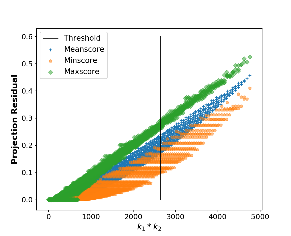
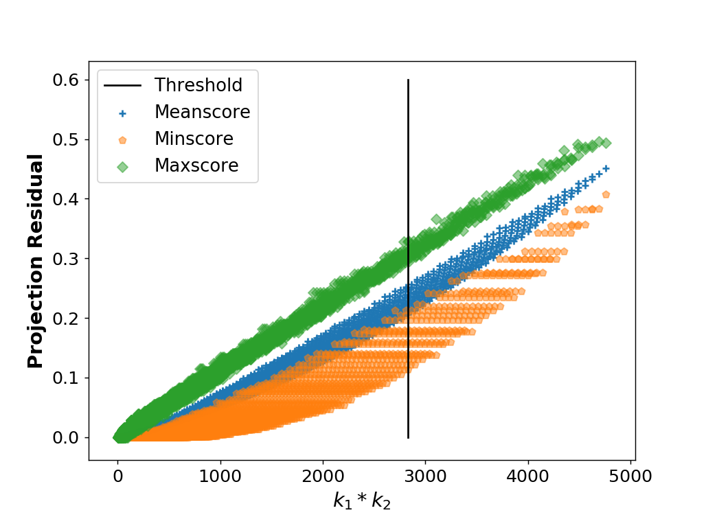
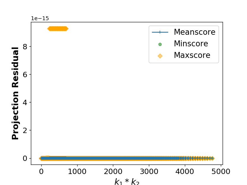
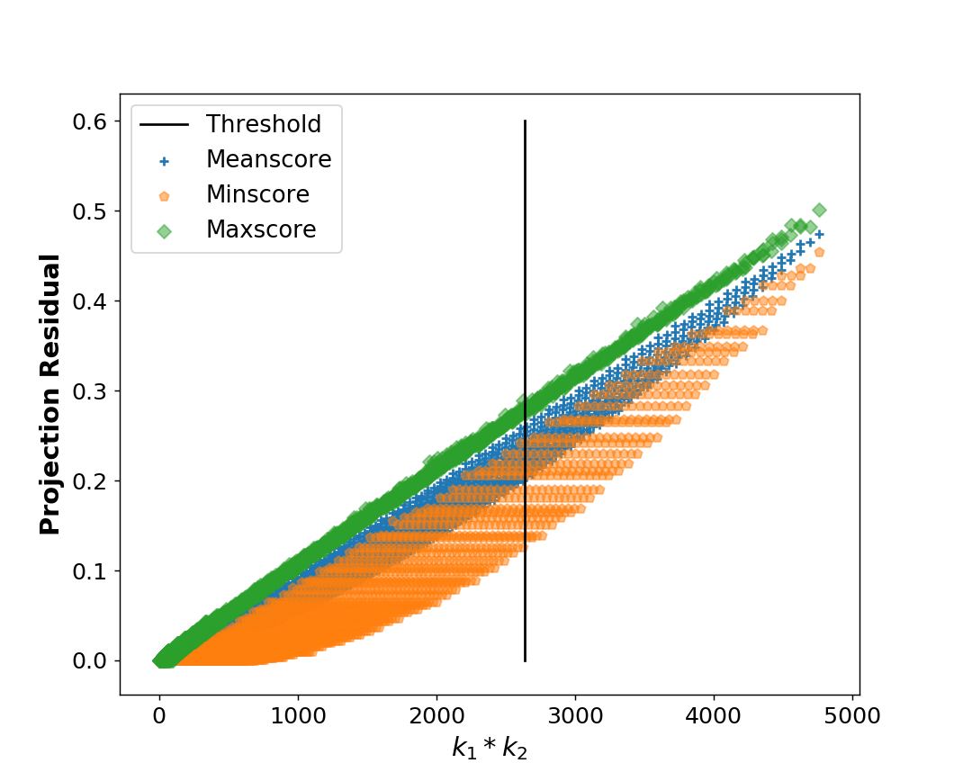
Figure 2: The projection residual β€–π˜Ξ©^βˆ’π”Ξ©^Aβ€‹π˜Ξ©^​𝐔Ω^Bβ€–F2superscriptsubscriptnormsubscript𝐘^Ξ©subscriptsuperscript𝐔𝐴^Ξ©subscript𝐘^Ξ©subscriptsuperscript𝐔𝐡^Ω𝐹2\left|\left|{\mathbf{Y}}_{\widehat{{\Omega}}}-{\mathbf{U}}^{A}_{\widehat{{\Omega}}}{\mathbf{Y}}_{\widehat{{\Omega}}}{\mathbf{U}}^{B}_{\widehat{{\Omega}}}\right|\right|_{F}^{2} averaged over 1000 simulations for fixed row π€βˆˆβ„k1Γ—10𝐀superscriptℝsubscriptπ‘˜110{\mathbf{A}}\in\mathbb{R}^{k_{1}\times 10} and column πβˆˆβ„k2Γ—10𝐁superscriptℝsubscriptπ‘˜210{\mathbf{B}}\in\mathbb{R}^{k_{2}\times 10} subspaces, fixed sample size defined by k1subscriptπ‘˜1k_{1} and k2subscriptπ‘˜2k_{2} but different set of samples Ξ©^^Ξ©\widehat{{\Omega}} drawn without replacement and signal dimension π˜βˆˆβ„100Γ—100𝐘superscriptℝ100100{\mathbf{Y}}\in\mathbb{R}^{100\times 100}.

For completeness, we carry out analysis on more general results, that is on Theorem 15, as all the properties which holds for the general case of missing signals are all applicable for the restricted problem as well. All the parameters Ξ±,Ξ²,Ξ³1𝛼𝛽subscript𝛾1\alpha,\beta,\gamma_{1} and Ξ³2subscript𝛾2\gamma_{2} depend on δ𝛿\delta and the lower bound of the Theorem 15 contains all these parameters. In order to get more information about the lower bound we set all these parameters very near to 00, therefore for a incoherent row and column subspace, that is for μ​(𝐀)=1πœ‡π€1\mu({\mathbf{A}})=1 and μ​(𝐁)=1πœ‡π1\mu({\mathbf{B}})=1 we write the lower bound as:

k1​m2+k2​m1βˆ’k1​k2m1​m2​(1βˆ’n1​m2+n2​m12​k1​k2)β€‹β€–π˜βˆ’π”Aβ€‹π˜π”Bβ€–F2.subscriptπ‘˜1subscriptπ‘š2subscriptπ‘˜2subscriptπ‘š1subscriptπ‘˜1subscriptπ‘˜2subscriptπ‘š1subscriptπ‘š21subscript𝑛1subscriptπ‘š2subscript𝑛2subscriptπ‘š12subscriptπ‘˜1subscriptπ‘˜2subscriptsuperscriptnorm𝐘superscript𝐔𝐴superscriptπ˜π”π΅2𝐹\frac{k_{1}m_{2}+k_{2}m_{1}-k_{1}k_{2}}{m_{1}m_{2}}\left(1-\frac{n_{1}m_{2}+n_{2}m_{1}}{2k_{1}k_{2}}\right)\\ \left|\left|{\mathbf{Y}}-{\mathbf{U}}^{A}{\mathbf{Y}}{\mathbf{U}}^{B}\right|\right|^{2}_{F}.

For k1<n1subscriptπ‘˜1subscript𝑛1k_{1}<n_{1} and k2<n2subscriptπ‘˜2subscript𝑛2k_{2}<n_{2}, the first term in the above expression k1​m2+k2​m1βˆ’k1​k2m1​m2>0subscriptπ‘˜1subscriptπ‘š2subscriptπ‘˜2subscriptπ‘š1subscriptπ‘˜1subscriptπ‘˜2subscriptπ‘š1subscriptπ‘š20\frac{k_{1}m_{2}+k_{2}m_{1}-k_{1}k_{2}}{m_{1}m_{2}}>0. It is because that the actual signal dimension m1subscriptπ‘š1m_{1} and m2subscriptπ‘š2m_{2} is greater than the corresponding row and column subspace dimensions n1subscript𝑛1n_{1} and n2subscript𝑛2n_{2}. Therefore for m1=m2=msubscriptπ‘š1subscriptπ‘š2π‘šm_{1}=m_{2}=m, n1=n2=nsubscript𝑛1subscript𝑛2𝑛n_{1}=n_{2}=n and k1=k2=ksubscriptπ‘˜1subscriptπ‘˜2π‘˜k_{1}=k_{2}=k we write the lower bound as:

2​k​(mβˆ’k)m2​(1βˆ’n​mk2)β€‹β€–π˜βˆ’π”Aβ€‹π˜π”Bβ€–F2.2π‘˜π‘šπ‘˜superscriptπ‘š21π‘›π‘šsuperscriptπ‘˜2subscriptsuperscriptnorm𝐘superscript𝐔𝐴superscriptπ˜π”π΅2𝐹\frac{2k(m-k)}{m^{2}}\left(1-\frac{nm}{k^{2}}\right)\left|\left|{\mathbf{Y}}-{\mathbf{U}}^{A}{\mathbf{Y}}{\mathbf{U}}^{B}\right|\right|^{2}_{F}.

Here the second term is always ≀0absent0\leq 0 as n​m>k2π‘›π‘šsuperscriptπ‘˜2nm>k^{2}. Therefore, for the incoherent row and column subspaces the lower bound is ≀0absent0\leq 0, which is consistent with the fact that β€–π˜Ξ©βˆ’π”Ξ©Aβ€‹π˜Ξ©β€‹π”Ξ©Bβ€–F2=0superscriptsubscriptnormsubscript𝐘Ωsubscriptsuperscript𝐔𝐴Ωsubscript𝐘Ωsubscriptsuperscript𝐔𝐡Ω𝐹20\left|\left|{\mathbf{Y}}_{\Omega}-{\mathbf{U}}^{A}_{\Omega}{\mathbf{Y}}_{\Omega}{\mathbf{U}}^{B}_{\Omega}\right|\right|_{F}^{2}=0 for k1<n1subscriptπ‘˜1subscript𝑛1k_{1}<n_{1} and k2<n2subscriptπ‘˜2subscript𝑛2k_{2}<n_{2}.

For the experiments, we choose highly incoherent subspaces. Both row and column subspaces have Gaussian random bases, that is μ​(𝐀)β‰ˆ1.3πœ‡π€1.3\mu({\mathbf{A}})\approx 1.3 and μ​(𝐁)β‰ˆ1.3πœ‡π1.3\mu({\mathbf{B}})\approx 1.3. In all these simulations in Fig. 2 we plot the residual energy β€–π˜Ξ©^βˆ’π”Ξ©^Aβ€‹π˜Ξ©^​𝐔Ω^Bβ€–F2superscriptsubscriptnormsubscript𝐘^Ξ©subscriptsuperscript𝐔𝐴^Ξ©subscript𝐘^Ξ©subscriptsuperscript𝐔𝐡^Ω𝐹2\left|\left|{\mathbf{Y}}_{\widehat{{\Omega}}}-{\mathbf{U}}^{A}_{\widehat{{\Omega}}}{\mathbf{Y}}_{\widehat{{\Omega}}}{\mathbf{U}}^{B}_{\widehat{{\Omega}}}\right|\right|_{F}^{2} as a function of k1β‹…k2β‹…subscriptπ‘˜1subscriptπ‘˜2k_{1}\cdot k_{2}. The plots show the maximum, minimum and mean values of the calculated residual energy over 1000 simulations of Ξ©^^Ξ©\widehat{{\Omega}} without replacement for fixed row and column subspace, fixed unit norm signal and 𝐘∈(π€βŠ—π)βŠ₯𝐘superscripttensor-product𝐀𝐁bottom{\mathbf{Y}}\in({\mathbf{A}}\otimes{\mathbf{B}})^{\bot} in Fig. 2(a). We find that the residual energy is always positive when k1β‰₯n1​μ​(𝐀)​log⁑(n1)subscriptπ‘˜1subscript𝑛1πœ‡π€subscript𝑛1k_{1}\geq n_{1}\mu({\mathbf{A}})\log\left(n_{1}\right) and k2β‰₯n2​μ​(𝐁)​log⁑(n2)subscriptπ‘˜2subscript𝑛2πœ‡πsubscript𝑛2k_{2}\geq n_{2}\mu({\mathbf{B}})\log\left(n_{2}\right). The threshold in the Fig. 2 is calculated as the product of lower bounds of k1subscriptπ‘˜1k_{1} and k2subscriptπ‘˜2k_{2}. In Fig. 2(b), 2(c) we also show that the residual energy is still positive when the signal is sampled from a Kronecker subspace with any one of the subspaces is orthogonal. As expected, the residual energy is 00 for the signal sampled from the Kronecker subspace itself, that is for 𝐘∈(π€βŠ—π)𝐘tensor-product𝐀𝐁{\mathbf{Y}}\in({\mathbf{A}}\otimes{\mathbf{B}}) the residual energy is 00, as shown in Fig. 2(d).

V Matched Subspace Detection

In the noise less case 𝐘=𝐀𝐗𝐁T𝐘superscript𝐀𝐗𝐁𝑇{\mathbf{Y}}={\mathbf{A}}{\mathbf{X}}{\mathbf{B}}^{T} we can assume Ξ·=0πœ‚0\eta=0; we form the detection setup for the hypotheses β„‹0:π˜βˆˆπƒ:subscriptβ„‹0π˜πƒ\mathcal{H}_{0}:{\mathbf{Y}}\in{\mathbf{D}} and β„‹1:π˜βˆ‰πƒ:subscriptβ„‹1π˜πƒ\mathcal{H}_{1}:{\mathbf{Y}}\notin{\mathbf{D}}. We use the following test statistics

β€–π˜Ξ©βˆ’π”Ξ©Aβ€‹π˜Ξ©β€‹π”Ξ©Bβ€–F2​≢ℋ1β„‹0​η.superscriptsubscriptnormsubscript𝐘Ωsuperscriptsubscript𝐔Ω𝐴subscript𝐘Ωsuperscriptsubscript𝐔Ω𝐡𝐹2subscriptβ„‹1subscriptβ„‹0less-than-or-greater-thanπœ‚\left|\left|{\mathbf{Y}}_{\Omega}-{\mathbf{U}}_{\Omega}^{A}{\mathbf{Y}}_{\Omega}{\mathbf{U}}_{\Omega}^{B}\right|\right|_{F}^{2}\underset{\mathcal{H}_{1}}{\overset{\mathcal{H}_{0}}{\lessgtr}}\eta. (18)

For the large enough values of k1subscriptπ‘˜1k_{1} and k2subscriptπ‘˜2k_{2} and Ξ΄>0𝛿0\delta>0 the probability of detection is greater than 1βˆ’8​δ18𝛿1-8\delta, that is ℙ​[β€–π˜Ξ©βˆ’π”Ξ©Aβ€‹π˜Ξ©β€‹π”Ξ©Bβ€–F2>0|β„‹1]β‰₯1βˆ’8​δℙdelimited-[]superscriptsubscriptnormsubscript𝐘Ωsuperscriptsubscript𝐔Ω𝐴subscript𝐘Ωsuperscriptsubscript𝐔Ω𝐡𝐹2conditional0subscriptβ„‹118𝛿\mathbb{P}\left[\left|\left|{\mathbf{Y}}_{\Omega}-{\mathbf{U}}_{\Omega}^{A}{\mathbf{Y}}_{\Omega}{\mathbf{U}}_{\Omega}^{B}\right|\right|_{F}^{2}>0\Big{|}\mathcal{H}_{1}\right]\geq 1-8\delta. Also, as shown in Fig. 2(d), the projection error is zero when the signal belongs to the Kronecker-structured subspace. Therefore, the probability of false alarm is also 0, ℙ​[β€–π˜Ξ©βˆ’π”Ξ©Aβ€‹π˜Ξ©β€‹π”Ξ©Bβ€–F2>0|β„‹0]=0β„™delimited-[]superscriptsubscriptnormsubscript𝐘Ωsuperscriptsubscript𝐔Ω𝐴subscript𝐘Ωsuperscriptsubscript𝐔Ω𝐡𝐹2conditional0subscriptβ„‹00\mathbb{P}\left[\left|\left|{\mathbf{Y}}_{\Omega}-{\mathbf{U}}_{\Omega}^{A}{\mathbf{Y}}_{\Omega}{\mathbf{U}}_{\Omega}^{B}\right|\right|_{F}^{2}>0\Big{|}\mathcal{H}_{0}\right]=0.

With the noisy signal 𝐘~=𝐀𝐗𝐁T+𝐙~𝐘superscript𝐀𝐗𝐁𝑇𝐙\widetilde{{\mathbf{Y}}}={\mathbf{A}}{\mathbf{X}}{\mathbf{B}}^{T}+\mathbf{Z}, where π™βˆΌπ’©β€‹(0,𝕀)similar-to𝐙𝒩0𝕀\mathbf{Z}\sim\mathcal{N}(0,\mathbb{I}), we use the same hypothesis but the test statistics changes to

β€–π˜~Ξ©βˆ’π”Ξ©Aβ€‹π˜~Ω​𝐔ΩBβ€–F2​≢ℋ1β„‹0​η.superscriptsubscriptnormsubscript~𝐘Ωsuperscriptsubscript𝐔Ω𝐴subscript~𝐘Ωsuperscriptsubscript𝐔Ω𝐡𝐹2subscriptβ„‹1subscriptβ„‹0less-than-or-greater-thanπœ‚\left|\left|\widetilde{{\mathbf{Y}}}_{\Omega}-{\mathbf{U}}_{\Omega}^{A}\widetilde{{\mathbf{Y}}}_{\Omega}{\mathbf{U}}_{\Omega}^{B}\right|\right|_{F}^{2}\underset{\mathcal{H}_{1}}{\overset{\mathcal{H}_{0}}{\lessgtr}}\eta. (19)

Here, we note that according to [7], the test statistics is distributed as a non-central 𝒳2superscript𝒳2\mathcal{X}^{2} with n1​n2subscript𝑛1subscript𝑛2n_{1}n_{2} degrees of freedom and the non-centrality parameter β€–π˜Ξ©βˆ’π”Ξ©Aβ€‹π˜Ξ©β€‹π”Ξ©Bβ€–F2superscriptsubscriptnormsubscript𝐘Ωsuperscriptsubscript𝐔Ω𝐴subscript𝐘Ωsuperscriptsubscript𝐔Ω𝐡𝐹2\left|\left|{\mathbf{Y}}_{\Omega}-{\mathbf{U}}_{\Omega}^{A}{\mathbf{Y}}_{\Omega}{\mathbf{U}}_{\Omega}^{B}\right|\right|_{F}^{2}, Where the detection probability Β PD=1βˆ’β„™β€‹[𝒳n1​n22​(β€–π˜Ξ©βˆ’π”Ξ©Aβ€‹π˜Ξ©β€‹π”Ξ©Bβ€–F2)≀η]subscript𝑃𝐷1β„™delimited-[]subscriptsuperscript𝒳2subscript𝑛1subscript𝑛2superscriptsubscriptnormsubscript𝐘Ωsuperscriptsubscript𝐔Ω𝐴subscript𝐘Ωsuperscriptsubscript𝐔Ω𝐡𝐹2πœ‚P_{D}=1-\mathbb{P}~{}\left[\mathcal{X}^{2}_{n_{1}n_{2}}\left(\left|\left|{\mathbf{Y}}_{\Omega}-{\mathbf{U}}_{\Omega}^{A}{\mathbf{Y}}_{\Omega}{\mathbf{U}}_{\Omega}^{B}\right|\right|_{F}^{2}\right)\leq\eta\right]Β  increases monotonically with the non-centrality parameter. Therefore, this means that the detection probability grows with either k1subscriptπ‘˜1k_{1} or k2subscriptπ‘˜2k_{2} or both.

VI Conclusion

In this paper, we extend the matched subspace detection for vectorized signals to tensor signals by projecting the signal onto Kronecker-structured subspace. We have further shown that the detection from a highly incomplete tensor signal is possible by computing the energy outside the KS subspace.

References

  • [1] Yeqing Li, Chen Chen, and Jungzhou Huang, β€œTransformation-invariant collaborative sub-representation,” in 2014 22nd International Conference on Pattern Recognition (ICPR). IEEE, 2014, pp. 3738–3743.
  • [2] Jun Wang and Kai Xu, β€œShape detection from raw lidar data with subspace modeling,” IEEE transactions on visualization and computer graphics, vol. 23, no. 9, pp. 2137–2150, 2017.
  • [3] Hadi Sarieddeen, MohammadΒ M Mansour, and Ali Chehab, β€œEfficient subspace detection for high-order mimo systems,” in Acoustics, Speech and Signal Processing (ICASSP), 2016 IEEE International Conference on. IEEE, 2016, pp. 1001–1005.
  • [4] MichaelΒ L McCloud and LouisΒ L Scharf, β€œInterference estimation with applications to blind multiple-access communication over fading channels,” IEEE Transactions on Information Theory, vol. 46, no. 3, pp. 947–961, 2000.
  • [5] EmmanuelΒ J CandΓ¨s and Benjamin Recht, β€œExact matrix completion via convex optimization,” Foundations of Computational mathematics, vol. 9, no. 6, pp. 717, 2009.
  • [6] Akshay Krishnamurthy and Aarti Singh, β€œLow-rank matrix and tensor completion via adaptive sampling,” in Advances in Neural Information Processing Systems, 2013, pp. 836–844.
  • [7] LouisΒ L Scharf and Benjamin Friedlander, β€œMatched subspace detectors,” IEEE Transactions on signal processing, vol. 42, no. 8, pp. 2146–2157, 1994.
  • [8] Martin Azizyan and Aarti Singh, β€œSubspace detection of high-dimensional vectors using compressive sampling,” in 2012 IEEE Statistical Signal Processing Workshop (SSP). IEEE, 2012, pp. 724–727.
  • [9] Laura Balzano, Benjamin Recht, and Robert Nowak, β€œHigh-dimensional matched subspace detection when data are missing,” in Information Theory Proceedings (ISIT), 2010 IEEE International Symposium on. IEEE, 2010, pp. 1638–1642.
  • [10] Tong Wu and WaheedΒ U Bajwa, β€œSubspace detection in a kernel space: The missing data case,” in Statistical Signal Processing (SSP), 2014 IEEE Workshop on. IEEE, 2014, pp. 93–96.
  • [11] Aalok Gangopadhyay, ShivamΒ Mani Tripathi, Ishan Jindal, and Shanmuganathan Raman, β€œDynamic scene classification using convolutional neural networks,” in Signal and Information Processing (GlobalSIP), 2016 IEEE Global Conference on. IEEE, 2016, pp. 1255–1259.
  • [12] Michael Elad and Michal Aharon, β€œImage denoising via sparse and redundant representations over learned dictionaries,” IEEE Transactions on Image processing, vol. 15, no. 12, pp. 3736–3745, 2006.
  • [13] Ishan Jindal and Matthew Nokleby, β€œPerformance limits on the classification of kronecker-structured models,” in Information Theory (ISIT), 2017 IEEE International Symposium on. IEEE, 2017, pp. 1998–2002.
  • [14] Mehdi Bahri, Yannis Panagakis, and Stefanos Zafeiriou, β€œRobust kronecker component analysis,” arXiv preprint arXiv:1801.06432, 2018.
  • [15] Ishan Jindal and Matthew Nokleby, β€œClassification and representation via separable subspaces: Performance limits and algorithms,” IEEE Journal of Selected Topics in Signal Processing, 2018.
  • [16] Colin McDiarmid, β€œOn the method of bounded differences. surveys in combinatorics, 1989 (norwich, 1989), 148–188,” London Math. Soc. Lecture Note Ser, vol. 141.
  • [17] PΒ Lancaster and HKΒ Farahat, β€œNorms on direct sums and tensor products,” mathematics of computation, vol. 26, no. 118, pp. 401–414, 1972.
  • [18] DennisΒ S Bernstein, Matrix mathematics: Theory, facts, and formulas with application to linear systems theory, vol.Β 41, Princeton university press Princeton, 2005.

Appendix A Concentration Inequalities

Theorem 3 (McDiarmid’s Inequality [16]).

Let X1,X2,β‹―,Xm1​m2subscript𝑋1subscript𝑋2β‹―subscript𝑋subscriptπ‘š1subscriptπ‘š2X_{1},X_{2},\cdots,X_{m_{1}m_{2}} be the independent random variables and assume a function f𝑓f, such that f​(X1,X2,β‹―,Xm1​m2):=Yassign𝑓subscript𝑋1subscript𝑋2β‹―subscript𝑋subscriptπ‘š1subscriptπ‘š2π‘Œf(X_{1},X_{2},\cdots,X_{m_{1}m_{2}}):=Y, then for Ο΅>0italic-Ο΅0\epsilon>0 there exists tisubscript𝑑𝑖t_{i} such that

ℙ​[Yβ‰₯E​[Y]+Ο΅]≀exp⁑(βˆ’2​ϡ2βˆ‘i=1m1​m2ti2),β„™delimited-[]π‘ŒπΈdelimited-[]π‘Œitalic-Ο΅2superscriptitalic-Ο΅2superscriptsubscript𝑖1subscriptπ‘š1subscriptπ‘š2superscriptsubscript𝑑𝑖2\mathbb{P}\left[Y\geq E[Y]+\epsilon\right]\leq\exp\left(\frac{-2\epsilon^{2}}{\sum_{i=1}^{m_{1}m_{2}}t_{i}^{2}}\right), (20)
ℙ​[Y≀E​[Y]βˆ’Ο΅]≀exp⁑(βˆ’2​ϡ2βˆ‘i=1m1​m2ti2).β„™delimited-[]π‘ŒπΈdelimited-[]π‘Œitalic-Ο΅2superscriptitalic-Ο΅2superscriptsubscript𝑖1subscriptπ‘š1subscriptπ‘š2superscriptsubscript𝑑𝑖2\mathbb{P}\left[Y\leq E[Y]-\epsilon\right]\leq\exp\left(\frac{-2\epsilon^{2}}{\sum_{i=1}^{m_{1}m_{2}}t_{i}^{2}}\right). (21)
Theorem 4 (Bernstein’s Inequality [9]).

Let 𝐗1,𝐗2,β‹―,𝐗msubscript𝐗1subscript𝐗2β‹―subscriptπ—π‘š{\mathbf{X}}_{1},{\mathbf{X}}_{2},\cdots,{\mathbf{X}}_{m} be the independent non-zero rΓ—rπ‘Ÿπ‘Ÿr\times r matrices and if for almost all kπ‘˜k, ρk2=max⁑{β€–E​[𝐗k​𝐗kT]β€–2,β€–E​[𝐗kT​𝐗k]β€–2}superscriptsubscriptπœŒπ‘˜2subscriptnorm𝐸delimited-[]subscriptπ—π‘˜superscriptsubscriptπ—π‘˜π‘‡2subscriptnorm𝐸delimited-[]superscriptsubscriptπ—π‘˜π‘‡subscriptπ—π‘˜2\rho_{k}^{2}=\max\{||E[{\mathbf{X}}_{k}{\mathbf{X}}_{k}^{T}]||_{2},||E[{\mathbf{X}}_{k}^{T}{\mathbf{X}}_{k}]||_{2}\} and ‖𝐗kβ€–2≀Msubscriptnormsubscriptπ—π‘˜2𝑀||{\mathbf{X}}_{k}||_{2}\leq M hold true, then for any Ο„>0𝜏0\tau>0,

ℙ​[β€–βˆ‘i=1m𝐗iβ€–2>Ο„]≀2​r​exp⁑(βˆ’Ο„2/2βˆ‘i=1mρk2+M​τ/3)β„™delimited-[]subscriptnormsuperscriptsubscript𝑖1π‘šsubscript𝐗𝑖2𝜏2π‘Ÿsuperscript𝜏22superscriptsubscript𝑖1π‘šsuperscriptsubscriptπœŒπ‘˜2π‘€πœ3\mathbb{P}\left[\left|\left|\sum_{i=1}^{m}{\mathbf{X}}_{i}\right|\right|_{2}>\tau\right]\leq 2r\exp\left(\frac{-\tau^{2}/2}{\sum_{i=1}^{m}\rho_{k}^{2}+M\tau/3}\right) (22)

Appendix B KS Coherence

Lemma 7.

The coherence of the Kronecker-structured subspace π€βŠ—πβˆˆβ„m1​m2Γ—n1​n2tensor-product𝐀𝐁superscriptℝsubscriptπ‘š1subscriptπ‘š2subscript𝑛1subscript𝑛2{{\mathbf{A}}\otimes{\mathbf{B}}\in\mathbb{R}^{m_{1}m_{2}\times n_{1}n_{2}}} is equal to the product of coherence of individual subspaces π€βˆˆπ‘m1Γ—n1𝐀superscript𝐑subscriptπ‘š1subscript𝑛1{\mathbf{A}}\in\mathbf{R}^{m_{1}\times n_{1}} and πβˆˆπ‘m2Γ—n2𝐁superscript𝐑subscriptπ‘š2subscript𝑛2{\mathbf{B}}\in\mathbf{R}^{m_{2}\times n_{2}}, that is

μ​(π€βŠ—π)=μ​(𝐀)​μ​(𝐁).πœ‡tensor-productπ€ππœ‡π€πœ‡π\mu({\mathbf{A}}\otimes{\mathbf{B}})=\mu({\mathbf{A}})\mu({\mathbf{B}}). (23)
Proof:

We write the coherence of Kronecker product of two subspaces as

μ​(π€βŠ—π)=m1​m2n1​n2​max𝑗​‖𝐔(π€βŠ—π)​ejA​Bβ€–22,πœ‡tensor-product𝐀𝐁subscriptπ‘š1subscriptπ‘š2subscript𝑛1subscript𝑛2𝑗maxsubscriptsuperscriptnormsuperscript𝐔tensor-product𝐀𝐁subscriptsuperscript𝑒𝐴𝐡𝑗22\displaystyle\mu({\mathbf{A}}\otimes{\mathbf{B}})=\frac{m_{1}m_{2}}{n_{1}n_{2}}\underset{j}{\text{max}}\left|\left|{\mathbf{U}}^{({\mathbf{A}}\otimes{\mathbf{B}})}e^{AB}_{j}\right|\right|^{2}_{2}, (24)

where 𝐔(π€βŠ—π)=(π€βŠ—π)​((π€βŠ—π)T​(π€βŠ—π))βˆ’1​(π€βŠ—π)Tsuperscript𝐔tensor-product𝐀𝐁tensor-product𝐀𝐁superscriptsuperscripttensor-product𝐀𝐁𝑇tensor-product𝐀𝐁1superscripttensor-product𝐀𝐁𝑇{\mathbf{U}}^{({\mathbf{A}}\otimes{\mathbf{B}})}=({\mathbf{A}}\otimes{\mathbf{B}})\left(({\mathbf{A}}\otimes{\mathbf{B}})^{T}({\mathbf{A}}\otimes{\mathbf{B}})\right)^{-1}({\mathbf{A}}\otimes{\mathbf{B}})^{T} is the orthogonal projector operator onto the Kronecker structured subspace (π€βŠ—π)tensor-product𝐀𝐁({\mathbf{A}}\otimes{\mathbf{B}}). We can use Kronecker product properties to further simplify this, as

𝐔(π€βŠ—π)superscript𝐔tensor-product𝐀𝐁\displaystyle{\mathbf{U}}^{({\mathbf{A}}\otimes{\mathbf{B}})} =(π€βŠ—π)​((π€βŠ—π)T​(π€βŠ—π))βˆ’1​(π€βŠ—π)Tabsenttensor-product𝐀𝐁superscriptsuperscripttensor-product𝐀𝐁𝑇tensor-product𝐀𝐁1superscripttensor-product𝐀𝐁𝑇\displaystyle=({\mathbf{A}}\otimes{\mathbf{B}})\left(({\mathbf{A}}\otimes{\mathbf{B}})^{T}({\mathbf{A}}\otimes{\mathbf{B}})\right)^{-1}({\mathbf{A}}\otimes{\mathbf{B}})^{T}
=(π€βŠ—π)​(𝐀Tβ€‹π€βŠ—πT​𝐁)βˆ’1​(π€βŠ—π)Tabsenttensor-product𝐀𝐁superscripttensor-productsuperscript𝐀𝑇𝐀superscript𝐁𝑇𝐁1superscripttensor-product𝐀𝐁𝑇\displaystyle=({\mathbf{A}}\otimes{\mathbf{B}})\left({\mathbf{A}}^{T}{\mathbf{A}}\otimes{\mathbf{B}}^{T}{\mathbf{B}}\right)^{-1}({\mathbf{A}}\otimes{\mathbf{B}})^{T}
=(𝐀​(𝐀T​𝐀)βˆ’1​𝐀T)βŠ—(𝐁​(𝐁T​𝐁)βˆ’1​𝐁T)absenttensor-product𝐀superscriptsuperscript𝐀𝑇𝐀1superscript𝐀𝑇𝐁superscriptsuperscript𝐁𝑇𝐁1superscript𝐁𝑇\displaystyle=({\mathbf{A}}({\mathbf{A}}^{T}{\mathbf{A}})^{-1}{\mathbf{A}}^{T})\otimes({\mathbf{B}}({\mathbf{B}}^{T}{\mathbf{B}})^{-1}{\mathbf{B}}^{T})
=𝐔AβŠ—π”B.absenttensor-productsuperscript𝐔𝐴superscript𝐔𝐡\displaystyle={\mathbf{U}}^{A}\otimes{\mathbf{U}}^{B}.

Therefore, we can write (24) as:

μ​(π€βŠ—π)πœ‡tensor-product𝐀𝐁\displaystyle\mu({\mathbf{A}}\otimes{\mathbf{B}}) =m1​m2n1​n2​max𝑗​‖(𝐔AβŠ—π”B)​ejA​Bβ€–22.absentsubscriptπ‘š1subscriptπ‘š2subscript𝑛1subscript𝑛2𝑗maxsubscriptsuperscriptnormtensor-productsuperscript𝐔𝐴superscript𝐔𝐡subscriptsuperscript𝑒𝐴𝐡𝑗22\displaystyle=\frac{m_{1}m_{2}}{n_{1}n_{2}}\underset{j}{\text{max}}\left|\left|({\mathbf{U}}^{A}\otimes{\mathbf{U}}^{B})e^{AB}_{j}\right|\right|^{2}_{2}. (25)

From [17], for the standard basis ejAsubscriptsuperscript𝑒𝐴𝑗e^{A}_{j} and ejBsubscriptsuperscript𝑒𝐡𝑗e^{B}_{j} with fixed degrees of freedom, we can always write ejA​B=ejAβŠ—ejBsubscriptsuperscript𝑒𝐴𝐡𝑗tensor-productsubscriptsuperscript𝑒𝐴𝑗subscriptsuperscript𝑒𝐡𝑗e^{AB}_{j}=e^{A}_{j}\otimes e^{B}_{j} . Thus,

μ​(π€βŠ—π)πœ‡tensor-product𝐀𝐁\displaystyle\mu({\mathbf{A}}\otimes{\mathbf{B}}) =m1​m2n1​n2​max𝑗​‖𝐔A​ejAβŠ—π”B​ejBβ€–22.absentsubscriptπ‘š1subscriptπ‘š2subscript𝑛1subscript𝑛2𝑗maxsubscriptsuperscriptnormtensor-productsuperscript𝐔𝐴subscriptsuperscript𝑒𝐴𝑗superscript𝐔𝐡subscriptsuperscript𝑒𝐡𝑗22\displaystyle=\frac{m_{1}m_{2}}{n_{1}n_{2}}\underset{j}{\text{max}}\left|\left|{\mathbf{U}}^{A}e^{A}_{j}\otimes{\mathbf{U}}^{B}e^{B}_{j}\right|\right|^{2}_{2}. (26)

We can further simplify the above equation using norm of Kronecker product property in [18]. that is, β€–π€βŠ—πβ€–2=‖𝐀‖2​‖𝐁‖2subscriptnormtensor-product𝐀𝐁2subscriptnorm𝐀2subscriptnorm𝐁2||{\mathbf{A}}\otimes{\mathbf{B}}||_{2}=||{\mathbf{A}}||_{2}||{\mathbf{B}}||_{2}. Finally, we can write

μ​(π€βŠ—π)πœ‡tensor-product𝐀𝐁\displaystyle\mu({\mathbf{A}}\otimes{\mathbf{B}}) =m1​m2n1​n2​max𝑗​(‖𝐔A​ejAβ€–22​‖𝐔B​ejBβ€–22)absentsubscriptπ‘š1subscriptπ‘š2subscript𝑛1subscript𝑛2𝑗maxsuperscriptsubscriptnormsuperscript𝐔𝐴subscriptsuperscript𝑒𝐴𝑗22subscriptsuperscriptnormsuperscript𝐔𝐡subscriptsuperscript𝑒𝐡𝑗22\displaystyle=\frac{m_{1}m_{2}}{n_{1}n_{2}}\underset{j}{\text{max}}\left(\left|\left|{\mathbf{U}}^{A}e^{A}_{j}\right|\right|_{2}^{2}\left|\left|{\mathbf{U}}^{B}e^{B}_{j}\right|\right|^{2}_{2}\right)
=m1​m2n1​n2​(max𝑗​‖𝐔A​ejAβ€–22)​(max𝑗​‖𝐔B​ejBβ€–22)absentsubscriptπ‘š1subscriptπ‘š2subscript𝑛1subscript𝑛2𝑗maxsuperscriptsubscriptnormsuperscript𝐔𝐴subscriptsuperscript𝑒𝐴𝑗22𝑗maxsubscriptsuperscriptnormsuperscript𝐔𝐡subscriptsuperscript𝑒𝐡𝑗22\displaystyle=\frac{m_{1}m_{2}}{n_{1}n_{2}}\left(\underset{j}{\text{max}}\left|\left|{\mathbf{U}}^{A}e^{A}_{j}\right|\right|_{2}^{2}\right)\left(\underset{j}{\text{max}}\left|\left|{\mathbf{U}}^{B}e^{B}_{j}\right|\right|^{2}_{2}\right)
=(m1n1​max𝑗​‖𝐔A​ejAβ€–22)​(m2n2​max𝑗​‖𝐔B​ejBβ€–22)absentsubscriptπ‘š1subscript𝑛1𝑗maxsuperscriptsubscriptnormsuperscript𝐔𝐴subscriptsuperscript𝑒𝐴𝑗22subscriptπ‘š2subscript𝑛2𝑗maxsubscriptsuperscriptnormsuperscript𝐔𝐡subscriptsuperscript𝑒𝐡𝑗22\displaystyle=\left(\frac{m_{1}}{n_{1}}\underset{j}{\text{max}}\left|\left|{\mathbf{U}}^{A}e^{A}_{j}\right|\right|_{2}^{2}\right)\left(\frac{m_{2}}{n_{2}}\underset{j}{\text{max}}\left|\left|{\mathbf{U}}^{B}e^{B}_{j}\right|\right|^{2}_{2}\right)
=μ​(𝐀)​μ​(𝐁).absentπœ‡π€πœ‡π\displaystyle=\mu({\mathbf{A}})\mu({\mathbf{B}}). (27)

∎

Appendix C Signal residual energy

Proof:

To prove this lemma we use Theorem 3 in Appendix A. Let |Ξ©A|=k1subscriptΩ𝐴subscriptπ‘˜1|\Omega_{A}|=k_{1} and |Ξ©B|=k2subscriptΩ𝐡subscriptπ‘˜2|\Omega_{B}|=k_{2} denotes the number of non-zero rows and columns. Therefore AΞ©βˆˆβ„k1Γ—n1subscript𝐴Ωsuperscriptℝsubscriptπ‘˜1subscript𝑛1A_{\Omega}\in\mathbb{R}^{k_{1}\times n_{1}} and BΞ©βˆˆβ„k2Γ—n2subscript𝐡Ωsuperscriptℝsubscriptπ‘˜2subscript𝑛2B_{\Omega}\in\mathbb{R}^{k_{2}\times n_{2}} and one can write β€–π˜β€–F2=12​(βˆ‘i=1m1β€–π˜β€‹(i,:)β€–22+βˆ‘j=1m2β€–π˜β€‹(:,j)β€–22)superscriptsubscriptnorm𝐘𝐹212superscriptsubscript𝑖1subscriptπ‘š1superscriptsubscriptnormπ˜π‘–:22superscriptsubscript𝑗1subscriptπ‘š2superscriptsubscriptnorm𝐘:𝑗22\left|\left|{\mathbf{Y}}\right|\right|_{F}^{2}=\frac{1}{2}\left(\sum_{i=1}^{m_{1}}\left|\left|{\mathbf{Y}}(i,:)\right|\right|_{2}^{2}+\sum_{j=1}^{m_{2}}\left|\left|{\mathbf{Y}}(:,j)\right|\right|_{2}^{2}\right). Set xi,j=π˜Ξ©β€‹(i,j)2subscriptπ‘₯𝑖𝑗subscriptsuperscript𝐘2Ω𝑖𝑗x_{i,j}={\mathbf{Y}}^{2}_{{\Omega}(i,j)} and we know that π˜Ξ©β€‹(i,j)2β‰€β€–π˜β€–βˆž2subscriptsuperscript𝐘2Ω𝑖𝑗superscriptsubscriptnorm𝐘2{\mathbf{Y}}^{2}_{{\Omega}(i,j)}\leq||{\mathbf{Y}}||_{\infty}^{2} is true βˆ€i∈{1,2,β‹―,k1}for-all𝑖12β‹―subscriptπ‘˜1\forall i\in\{1,2,\cdots,k_{1}\} and βˆ€j∈{1,2,β‹―,k2}for-all𝑗12β‹―subscriptπ‘˜2\forall j\in\{1,2,\cdots,k_{2}\}. Therefore,

E​[βˆ‘i=1k1βˆ‘j=1k2xi,j]𝐸delimited-[]superscriptsubscript𝑖1subscriptπ‘˜1superscriptsubscript𝑗1subscriptπ‘˜2subscriptπ‘₯𝑖𝑗\displaystyle E\left[\sum_{i=1}^{k_{1}}\sum_{j=1}^{k_{2}}x_{i,j}\right] =E​[β€–π˜β€–F2]βˆ’E​[βˆ‘i=1m1βˆ’k1β€–π˜Ξ©β€‹(i,:)β€–22+βˆ‘j=1m2βˆ’k2β€–π˜Ξ©β€‹(:,j)β€–22βˆ’βˆ‘i=1m1βˆ’k1βˆ‘j=1m2βˆ’k2(π˜Ξ©β€‹(i,j))2]absent𝐸delimited-[]superscriptsubscriptnorm𝐘𝐹2𝐸delimited-[]superscriptsubscript𝑖1subscriptπ‘š1subscriptπ‘˜1superscriptsubscriptnormsubscriptπ˜Ξ©π‘–:22superscriptsubscript𝑗1subscriptπ‘š2subscriptπ‘˜2superscriptsubscriptnormsubscript𝐘Ω:𝑗22superscriptsubscript𝑖1subscriptπ‘š1subscriptπ‘˜1superscriptsubscript𝑗1subscriptπ‘š2subscriptπ‘˜2superscriptsubscriptπ˜Ξ©π‘–π‘—2\displaystyle=E\left[||{\mathbf{Y}}||_{F}^{2}\right]-E\left[\sum_{i=1}^{m_{1}-k_{1}}||{\mathbf{Y}}_{\Omega}(i,:)||_{2}^{2}+\sum_{j=1}^{m_{2}-k_{2}}||{\mathbf{Y}}_{\Omega}(:,j)||_{2}^{2}-\sum_{i=1}^{m_{1}-k_{1}}\sum_{j=1}^{m_{2}-k_{2}}({\mathbf{Y}}_{\Omega}(i,j))^{2}\right]
=||𝐘||F2βˆ’(βˆ‘i=1m1βˆ’k1E[βˆ‘l=1m1||𝐘(i,:)||22πŸ™Ξ©β€‹(i,:)=l]+βˆ‘j=1m2βˆ’k2E[βˆ‘l=1m2||𝐘(:,j)||22πŸ™Ξ©β€‹(:,j)=l]\displaystyle=||{\mathbf{Y}}||_{F}^{2}-\Bigg{(}\sum_{i=1}^{m_{1}-k_{1}}E\left[\sum_{l=1}^{m_{1}}||{\mathbf{Y}}(i,:)||_{2}^{2}\mathbb{1}_{\Omega(i,:)=l}\right]+\sum_{j=1}^{m_{2}-k_{2}}E\left[\sum_{l=1}^{m_{2}}||{\mathbf{Y}}(:,j)||_{2}^{2}\mathbb{1}_{\Omega(:,j)=l}\right]
βˆ’βˆ‘i=1k1βˆ‘j=1k2E[βˆ‘r=1m1βˆ‘s=1m2(𝐘Ω(i,j))2πŸ™Ξ©β€‹(i,j)=(r,s)])\displaystyle\quad-\sum_{i=1}^{k_{1}}\sum_{j=1}^{k_{2}}E\left[\sum_{r=1}^{m_{1}}\sum_{s=1}^{m_{2}}({\mathbf{Y}}_{\Omega}(i,j))^{2}\mathbb{1}_{\Omega(i,j)=(r,s)}\right]\Bigg{)}
=β€–π˜β€–F2βˆ’[m1βˆ’k1m1β€‹β€–π˜β€–F2+m2βˆ’k2m2β€‹β€–π˜β€–F2βˆ’(m1βˆ’k1)​(m2βˆ’k2)m1​m2β€‹β€–π˜β€–F2]absentsuperscriptsubscriptnorm𝐘𝐹2delimited-[]subscriptπ‘š1subscriptπ‘˜1subscriptπ‘š1superscriptsubscriptnorm𝐘𝐹2subscriptπ‘š2subscriptπ‘˜2subscriptπ‘š2superscriptsubscriptnorm𝐘𝐹2subscriptπ‘š1subscriptπ‘˜1subscriptπ‘š2subscriptπ‘˜2subscriptπ‘š1subscriptπ‘š2superscriptsubscriptnorm𝐘𝐹2\displaystyle=||{\mathbf{Y}}||_{F}^{2}-\left[\frac{m_{1}-k_{1}}{m_{1}}||{\mathbf{Y}}||_{F}^{2}+\frac{m_{2}-k_{2}}{m_{2}}||{\mathbf{Y}}||_{F}^{2}-\frac{(m_{1}-k_{1})(m_{2}-k_{2})}{m_{1}m_{2}}||{\mathbf{Y}}||_{F}^{2}\right]
=[1βˆ’(m1βˆ’k1m1+m2βˆ’k2m2βˆ’(m1βˆ’k1)​(m2βˆ’k2)m1​m2)]β€‹β€–π˜β€–F2absentdelimited-[]1subscriptπ‘š1subscriptπ‘˜1subscriptπ‘š1subscriptπ‘š2subscriptπ‘˜2subscriptπ‘š2subscriptπ‘š1subscriptπ‘˜1subscriptπ‘š2subscriptπ‘˜2subscriptπ‘š1subscriptπ‘š2superscriptsubscriptnorm𝐘𝐹2\displaystyle=\left[1-\left(\frac{m_{1}-k_{1}}{m_{1}}+\frac{m_{2}-k_{2}}{m_{2}}-\frac{(m_{1}-k_{1})(m_{2}-k_{2})}{m_{1}m_{2}}\right)\right]||{\mathbf{Y}}||_{F}^{2}
=(k1​k2m1​m2)β€‹β€–π˜β€–F2,absentsubscriptπ‘˜1subscriptπ‘˜2subscriptπ‘š1subscriptπ‘š2superscriptsubscriptnorm𝐘𝐹2\displaystyle=\left(\frac{k_{1}k_{2}}{m_{1}m_{2}}\right)||{\mathbf{Y}}||_{F}^{2}, (28)

where πŸ™double-struck-πŸ™\mathbb{1} represents the indicator function and ΩΩ{\Omega} assumes that the samples are taken uniformly without replacement. Thus, from we write the left hand side of (21) as

ℙ​[|βˆ‘i=1k1βˆ‘j=1k2xi,j|≀E​[βˆ‘i=1k1βˆ‘j=1k2xi,j]βˆ’Ο΅]=ℙ​[|βˆ‘i=1k1βˆ‘j=1k2xi,j|≀(k1​k2m1​m2)β€‹β€–π˜β€–F2βˆ’Ο΅].β„™delimited-[]superscriptsubscript𝑖1subscriptπ‘˜1superscriptsubscript𝑗1subscriptπ‘˜2subscriptπ‘₯𝑖𝑗𝐸delimited-[]superscriptsubscript𝑖1subscriptπ‘˜1superscriptsubscript𝑗1subscriptπ‘˜2subscriptπ‘₯𝑖𝑗italic-Ο΅β„™delimited-[]superscriptsubscript𝑖1subscriptπ‘˜1superscriptsubscript𝑗1subscriptπ‘˜2subscriptπ‘₯𝑖𝑗subscriptπ‘˜1subscriptπ‘˜2subscriptπ‘š1subscriptπ‘š2superscriptsubscriptnorm𝐘𝐹2italic-Ο΅\mathbb{P}\left[\left|\sum_{i=1}^{k_{1}}\sum_{j=1}^{k_{2}}x_{i,j}\right|\leq E\left[\sum_{i=1}^{k_{1}}\sum_{j=1}^{k_{2}}x_{i,j}\right]-\epsilon\right]=\mathbb{P}\left[\left|\sum_{i=1}^{k_{1}}\sum_{j=1}^{k_{2}}x_{i,j}\right|\leq\left(\frac{k_{1}k_{2}}{m_{1}m_{2}}\right)\left|\left|{\mathbf{Y}}\right|\right|_{F}^{2}-\epsilon\right].

For Ο΅=α​(k1​k2m1​m2)β€‹β€–π˜β€–F2italic-ϡ𝛼subscriptπ‘˜1subscriptπ‘˜2subscriptπ‘š1subscriptπ‘š2superscriptsubscriptnorm𝐘𝐹2\epsilon=\alpha\left(\frac{k_{1}k_{2}}{m_{1}m_{2}}\right)\left|\left|{\mathbf{Y}}\right|\right|_{F}^{2}, we can bound this probability by

2​exp⁑(βˆ’2​(α​(k1​k2m1​m2)β€‹β€–π˜β€–F2)2βˆ‘i=1k1​k2(2β€‹β€–π˜β€–βˆž2)2)22superscript𝛼subscriptπ‘˜1subscriptπ‘˜2subscriptπ‘š1subscriptπ‘š2superscriptsubscriptnorm𝐘𝐹22superscriptsubscript𝑖1subscriptπ‘˜1subscriptπ‘˜2superscript2superscriptsubscriptnorm𝐘22\displaystyle 2\exp\left(\frac{-2\left(\alpha\left(\frac{k_{1}k_{2}}{m_{1}m_{2}}\right)\left|\left|{\mathbf{Y}}\right|\right|_{F}^{2}\right)^{2}}{\sum_{i=1}^{k_{1}k_{2}}\left(2||{\mathbf{Y}}||_{\infty}^{2}\right)^{2}}\right) =2​exp⁑(βˆ’2​α2​(k1​k2m1​m2)2β€‹β€–π˜β€–F44​k1​k2β€‹β€–π˜β€–βˆž4)absent22superscript𝛼2superscriptsubscriptπ‘˜1subscriptπ‘˜2subscriptπ‘š1subscriptπ‘š22superscriptsubscriptnorm𝐘𝐹44subscriptπ‘˜1subscriptπ‘˜2superscriptsubscriptnorm𝐘4\displaystyle=2\exp\left(\frac{-2\alpha^{2}\left(\frac{k_{1}k_{2}}{m_{1}m_{2}}\right)^{2}\left|\left|{\mathbf{Y}}\right|\right|_{F}^{4}}{4k_{1}k_{2}||{\mathbf{Y}}||_{\infty}^{4}}\right)
=2​exp⁑(βˆ’Ξ±2​(k1​k2)2​(β€–π˜β€–F2m1​m2β€‹β€–π˜β€–βˆž2)2)absent2superscript𝛼2subscriptπ‘˜1subscriptπ‘˜22superscriptsuperscriptsubscriptnorm𝐘𝐹2subscriptπ‘š1subscriptπ‘š2superscriptsubscriptnorm𝐘22\displaystyle=2\exp\left(\frac{-\alpha^{2}\left(k_{1}k_{2}\right)}{2}\left(\frac{\left|\left|{\mathbf{Y}}\right|\right|_{F}^{2}}{m_{1}m_{2}||{\mathbf{Y}}||_{\infty}^{2}}\right)^{2}\right)
=2​exp⁑(βˆ’Ξ±2​(k1​k2)2​μ​(𝐘)2).absent2superscript𝛼2subscriptπ‘˜1subscriptπ‘˜22πœ‡superscript𝐘2\displaystyle=2\exp\left(\frac{-\alpha^{2}\left(k_{1}k_{2}\right)}{2\mu({\mathbf{Y}})^{2}}\right).

The final bound obtained is:

ℙ​[π˜Ξ©β€‹(i,j)2β‰₯(1βˆ’Ξ±)​(k1​k2m1​m2)β€‹β€–π˜β€–F2]β‰₯1βˆ’2​exp⁑(βˆ’Ξ±2​(k1​k2)2​μ​(𝐘)2).β„™delimited-[]subscriptsuperscript𝐘2Ω𝑖𝑗1𝛼subscriptπ‘˜1subscriptπ‘˜2subscriptπ‘š1subscriptπ‘š2superscriptsubscriptnorm𝐘𝐹212superscript𝛼2subscriptπ‘˜1subscriptπ‘˜22πœ‡superscript𝐘2\mathbb{P}\left[{\mathbf{Y}}^{2}_{{\Omega}(i,j)}\geq(1-\alpha)\left(\frac{k_{1}k_{2}}{m_{1}m_{2}}\right)\left|\left|{\mathbf{Y}}\right|\right|_{F}^{2}\right]\geq 1-2\exp\left(\frac{-\alpha^{2}\left(k_{1}k_{2}\right)}{2\mu({\mathbf{Y}})^{2}}\right).

Then for Ξ±=2​μ​(𝐘)2k1​k2​log⁑(1Ξ΄)𝛼2πœ‡superscript𝐘2subscriptπ‘˜1subscriptπ‘˜21𝛿\alpha=\sqrt{\frac{2\mu({\mathbf{Y}})^{2}}{k_{1}k_{2}}\log(\frac{1}{\delta})}, with the probability 1βˆ’2​δ12𝛿1-2\delta:

(1βˆ’Ξ±)​(k1​k2m1​m2)β€‹β€–π˜β€–F2β‰€β€–π˜Ξ©β€–F2≀(1+Ξ±)​(k1​k2m1​m2)β€‹β€–π˜β€–F2.1𝛼subscriptπ‘˜1subscriptπ‘˜2subscriptπ‘š1subscriptπ‘š2superscriptsubscriptnorm𝐘𝐹2superscriptsubscriptnormsubscript𝐘Ω𝐹21𝛼subscriptπ‘˜1subscriptπ‘˜2subscriptπ‘š1subscriptπ‘š2superscriptsubscriptnorm𝐘𝐹2(1-\alpha)\left(\frac{k_{1}k_{2}}{m_{1}m_{2}}\right)||{\mathbf{Y}}||_{F}^{2}\leq||{\mathbf{Y}}_{\Omega}||_{F}^{2}\\ \leq(1+\alpha)\left(\frac{k_{1}k_{2}}{m_{1}m_{2}}\right)||{\mathbf{Y}}||_{F}^{2}. (29)

∎

Proof:

To prove this lemma we again use Theorem 3 in Appendix A and Lemma 23 in Appendix B. Let 𝐕Ωi,j=𝐀Ωi,:Tβ€‹π˜Ξ©i,j​𝐁Ω:,jsubscript𝐕subscriptΩ𝑖𝑗superscriptsubscript𝐀subscriptΩ𝑖:𝑇subscript𝐘subscriptΩ𝑖𝑗subscript𝐁subscriptΞ©:𝑗\mathbf{V}_{\Omega_{i,j}}={\mathbf{A}}_{\Omega_{i,:}}^{T}{\mathbf{Y}}_{\Omega_{i,j}}{\mathbf{B}}_{\Omega_{:,j}} represent the (i,j)t​hsuperscriptπ‘–π‘—π‘‘β„Ž(i,j)^{th} samples index, where Ξ©i,:subscriptΩ𝑖:{\Omega_{i,:}} represents the it​hsuperscriptπ‘–π‘‘β„Ži^{th} row of the column subspace 𝐀𝐀{\mathbf{A}} and Ξ©:,jsubscriptΞ©:𝑗{\Omega_{:,j}} represents the jt​hsuperscriptπ‘—π‘‘β„Žj^{th} row of the row subspace 𝐁𝐁{\mathbf{B}}. Here β€–βˆ‘i=1k1βˆ‘j=1k2𝐕Ωi,jβ€–F=‖𝐀ΩTβ€‹π˜Ξ©β€‹πΞ©β€–Fsubscriptnormsuperscriptsubscript𝑖1subscriptπ‘˜1superscriptsubscript𝑗1subscriptπ‘˜2subscript𝐕subscriptΩ𝑖𝑗𝐹subscriptnormsuperscriptsubscript𝐀Ω𝑇subscript𝐘Ωsubscript𝐁Ω𝐹\left|\left|\sum_{i=1}^{k_{1}}\sum_{j=1}^{k_{2}}\mathbf{V}_{\Omega_{i,j}}\right|\right|_{F}=\left|\left|{\mathbf{A}}_{\Omega}^{T}{\mathbf{Y}}_{\Omega}{\mathbf{B}}_{\Omega}\right|\right|_{F}. Now, in order to bound β€–Vβ€–norm𝑉||V|| we use the vectorized form of the signal and write ‖𝐀ΩTβ€‹π˜Ξ©β€‹πΞ©β€–F=‖𝐯‖2=β€–(π€βŠ—π)Ω​𝐲‖2=‖𝐃Ω​𝐲‖2subscriptnormsuperscriptsubscript𝐀Ω𝑇subscript𝐘Ωsubscript𝐁Ω𝐹subscriptnorm𝐯2subscriptnormsubscripttensor-product𝐀𝐁Ω𝐲2subscriptnormsubscript𝐃Ω𝐲2\left|\left|{\mathbf{A}}_{\Omega}^{T}{\mathbf{Y}}_{\Omega}{\mathbf{B}}_{\Omega}\right|\right|_{F}=||\mathbf{v}||_{2}=\left|\left|({\mathbf{A}}\otimes{\mathbf{B}})_{{\Omega}}\mathbf{y}\right|\right|_{2}=||{\mathbf{D}}_{{\Omega}}\mathbf{y}||_{2}, where 𝐲=vec​(𝐘)𝐲vec𝐘\mathbf{y}=\text{vec}({\mathbf{Y}}). By definition in (2), we know ‖𝐃Ω​(i)β€–2=‖𝐃T​eiβ€–2=‖𝐔𝐃​ejA​Bβ€–2≀n1​n2m1​m2​μ​(𝐃)subscriptnormsubscript𝐃Ω𝑖2subscriptnormsuperscript𝐃𝑇subscript𝑒𝑖2subscriptnormsuperscript𝐔𝐃subscriptsuperscript𝑒𝐴𝐡𝑗2subscript𝑛1subscript𝑛2subscriptπ‘š1subscriptπ‘š2πœ‡πƒ||{\mathbf{D}}_{{\Omega}(i)}||_{2}=||{\mathbf{D}}^{T}e_{i}||_{2}=\left|\left|{\mathbf{U}}^{{\mathbf{D}}}e^{AB}_{j}\right|\right|_{2}\leq\sqrt{\frac{n_{1}n_{2}}{m_{1}m_{2}}\mu({\mathbf{D}})}. Now from Lemma 23 we prove that the coherence of Kronecker subspace is product of coherence of individual subspaces. Therefore, we write ‖𝐃Ω​(i)β€–2≀n1​n2m1​m2​μ​(𝐀)​μ​(𝐁)subscriptnormsubscript𝐃Ω𝑖2subscript𝑛1subscript𝑛2subscriptπ‘š1subscriptπ‘š2πœ‡π€πœ‡π||{\mathbf{D}}_{{\Omega}(i)}||_{2}\leq\sqrt{\frac{n_{1}n_{2}}{m_{1}m_{2}}\mu({\mathbf{A}})\mu({\mathbf{B}})}. Thus, in vectorized form we write

‖𝐯iβ€–2≀|𝐲Ω​(i)|​‖𝐃Ω​(i)β€–2β‰€β€–π˜β€–βˆžβ€‹n1​n2m1​m2​μ​(𝐀)​μ​(𝐁).subscriptnormsubscript𝐯𝑖2subscript𝐲Ω𝑖subscriptnormsubscript𝐃Ω𝑖2subscriptnorm𝐘subscript𝑛1subscript𝑛2subscriptπ‘š1subscriptπ‘š2πœ‡π€πœ‡π||\mathbf{v}_{i}||_{2}\leq|\mathbf{y}_{{\Omega}(i)}|||{\mathbf{D}}_{{\Omega}(i)}||_{2}\leq||{\mathbf{Y}}||_{\infty}\sqrt{\frac{n_{1}n_{2}}{m_{1}m_{2}}\mu({\mathbf{A}})\mu({\mathbf{B}})}.

Now suppose that the samples are take uniformly without replacement, then we can write the following bound as

E​[β€–βˆ‘i=1k1βˆ‘j=1k2𝐕Ωi,jβ€–F2]𝐸delimited-[]superscriptsubscriptnormsuperscriptsubscript𝑖1subscriptπ‘˜1superscriptsubscript𝑗1subscriptπ‘˜2subscript𝐕subscriptΩ𝑖𝑗𝐹2\displaystyle E\left[\left|\left|\sum_{i=1}^{k_{1}}\sum_{j=1}^{k_{2}}\mathbf{V}_{\Omega_{i,j}}\right|\right|_{F}^{2}\right] =E​[β€–βˆ‘i=1k1βˆ‘j=1k2𝐀Ωi,:Tβ€‹π˜Ξ©i,j​𝐁Ω:,jβ€–F2]absent𝐸delimited-[]superscriptsubscriptnormsuperscriptsubscript𝑖1subscriptπ‘˜1superscriptsubscript𝑗1subscriptπ‘˜2superscriptsubscript𝐀subscriptΩ𝑖:𝑇subscript𝐘subscriptΩ𝑖𝑗subscript𝐁subscriptΞ©:𝑗𝐹2\displaystyle=E\left[\left|\left|\sum_{i=1}^{k_{1}}\sum_{j=1}^{k_{2}}{\mathbf{A}}_{\Omega_{i,:}}^{T}{\mathbf{Y}}_{\Omega_{i,j}}{\mathbf{B}}_{\Omega_{:,j}}\right|\right|_{F}^{2}\right]
=βˆ‘p=1n1βˆ‘q=1n2E​[βˆ‘i=1k1βˆ‘j=1k2βˆ‘r=1m1βˆ‘s=1m2𝐀r​p2β€‹π˜r​s2​(πŸ™r=i,s=j)​Bs​q2]absentsuperscriptsubscript𝑝1subscript𝑛1superscriptsubscriptπ‘ž1subscript𝑛2𝐸delimited-[]superscriptsubscript𝑖1subscriptπ‘˜1superscriptsubscript𝑗1subscriptπ‘˜2superscriptsubscriptπ‘Ÿ1subscriptπ‘š1superscriptsubscript𝑠1subscriptπ‘š2subscriptsuperscript𝐀2π‘Ÿπ‘subscriptsuperscript𝐘2π‘Ÿπ‘ subscriptdouble-struck-πŸ™formulae-sequenceπ‘Ÿπ‘–π‘ π‘—subscriptsuperscript𝐡2π‘ π‘ž\displaystyle=\sum_{p=1}^{n_{1}}\sum_{q=1}^{n_{2}}E\left[\sum_{i=1}^{k_{1}}\sum_{j=1}^{k_{2}}\sum_{r=1}^{m_{1}}\sum_{s=1}^{m_{2}}{\mathbf{A}}^{2}_{rp}{\mathbf{Y}}^{2}_{rs}(\mathbb{1}_{r=i,s=j})B^{2}_{sq}\right]
=βˆ‘p=1n1βˆ‘q=1n2k1​k2m1​m2​(βˆ‘r=1m1βˆ‘s=1m2𝐀r​p2β€‹π˜r​s2​𝐁s​q2)absentsuperscriptsubscript𝑝1subscript𝑛1superscriptsubscriptπ‘ž1subscript𝑛2subscriptπ‘˜1subscriptπ‘˜2subscriptπ‘š1subscriptπ‘š2superscriptsubscriptπ‘Ÿ1subscriptπ‘š1superscriptsubscript𝑠1subscriptπ‘š2subscriptsuperscript𝐀2π‘Ÿπ‘subscriptsuperscript𝐘2π‘Ÿπ‘ subscriptsuperscript𝐁2π‘ π‘ž\displaystyle=\sum_{p=1}^{n_{1}}\sum_{q=1}^{n_{2}}\frac{k_{1}k_{2}}{m_{1}m_{2}}\left(\sum_{r=1}^{m_{1}}\sum_{s=1}^{m_{2}}{\mathbf{A}}^{2}_{rp}{\mathbf{Y}}^{2}_{rs}{\mathbf{B}}^{2}_{sq}\right)
=βˆ‘p=1n1βˆ‘q=1n212​k1​k2m1​m2​(βˆ‘r=1m1βˆ‘s=1m2𝐀r​p2β€‹π˜r​s2+βˆ‘r=1m1βˆ‘s=1m2𝐘r​s2​𝐁s​q2)absentsuperscriptsubscript𝑝1subscript𝑛1superscriptsubscriptπ‘ž1subscript𝑛212subscriptπ‘˜1subscriptπ‘˜2subscriptπ‘š1subscriptπ‘š2superscriptsubscriptπ‘Ÿ1subscriptπ‘š1superscriptsubscript𝑠1subscriptπ‘š2subscriptsuperscript𝐀2π‘Ÿπ‘subscriptsuperscript𝐘2π‘Ÿπ‘ superscriptsubscriptπ‘Ÿ1subscriptπ‘š1superscriptsubscript𝑠1subscriptπ‘š2subscriptsuperscript𝐘2π‘Ÿπ‘ subscriptsuperscript𝐁2π‘ π‘ž\displaystyle=\sum_{p=1}^{n_{1}}\sum_{q=1}^{n_{2}}\frac{1}{2}\frac{k_{1}k_{2}}{m_{1}m_{2}}\left(\sum_{r=1}^{m_{1}}\sum_{s=1}^{m_{2}}{\mathbf{A}}^{2}_{rp}{\mathbf{Y}}^{2}_{rs}+\sum_{r=1}^{m_{1}}\sum_{s=1}^{m_{2}}{\mathbf{Y}}^{2}_{rs}{\mathbf{B}}^{2}_{sq}\right)
≀k1​k22​m1​m2​(n1m1​μ​(𝐀)+n2m2​μ​(𝐁))β€‹β€–π˜β€–F2.absentsubscriptπ‘˜1subscriptπ‘˜22subscriptπ‘š1subscriptπ‘š2subscript𝑛1subscriptπ‘š1πœ‡π€subscript𝑛2subscriptπ‘š2πœ‡πsubscriptsuperscriptnorm𝐘2𝐹\displaystyle\leq\frac{k_{1}k_{2}}{2m_{1}m_{2}}\left(\frac{n_{1}}{m_{1}}\mu({\mathbf{A}})+\frac{n_{2}}{m_{2}}\mu({\mathbf{B}})\right)||{\mathbf{Y}}||^{2}_{F}. (30)

Using the McDiard’s concentration inequality from Theorem 3, we write the left hand side of (20) as

ℙ​[β€–βˆ‘i=1k1βˆ‘j=1k2𝐕Ωi,jβ€–F2β‰₯E​[β€–βˆ‘i=1k1βˆ‘j=1k2𝐕Ωi,jβ€–F2]+Ο΅]=ℙ​[β€–βˆ‘i=1k1βˆ‘j=1k2𝐕Ωi,jβ€–F2β‰₯k1​k22​m1​m2​(n1m1​μ​(𝐀)+n2m2​μ​(𝐁))β€‹β€–π˜β€–F2+Ο΅].β„™delimited-[]superscriptsubscriptnormsuperscriptsubscript𝑖1subscriptπ‘˜1superscriptsubscript𝑗1subscriptπ‘˜2subscript𝐕subscriptΩ𝑖𝑗𝐹2𝐸delimited-[]superscriptsubscriptnormsuperscriptsubscript𝑖1subscriptπ‘˜1superscriptsubscript𝑗1subscriptπ‘˜2subscript𝐕subscriptΩ𝑖𝑗𝐹2italic-Ο΅β„™delimited-[]superscriptsubscriptnormsuperscriptsubscript𝑖1subscriptπ‘˜1superscriptsubscript𝑗1subscriptπ‘˜2subscript𝐕subscriptΩ𝑖𝑗𝐹2subscriptπ‘˜1subscriptπ‘˜22subscriptπ‘š1subscriptπ‘š2subscript𝑛1subscriptπ‘š1πœ‡π€subscript𝑛2subscriptπ‘š2πœ‡πsubscriptsuperscriptnorm𝐘2𝐹italic-Ο΅\mathbb{P}\left[\left|\left|\sum_{i=1}^{k_{1}}\sum_{j=1}^{k_{2}}\mathbf{V}_{\Omega_{i,j}}\right|\right|_{F}^{2}\geq E\left[\left|\left|\sum_{i=1}^{k_{1}}\sum_{j=1}^{k_{2}}\mathbf{V}_{\Omega_{i,j}}\right|\right|_{F}^{2}\right]+\epsilon\right]=\\ \mathbb{P}\left[\left|\left|\sum_{i=1}^{k_{1}}\sum_{j=1}^{k_{2}}\mathbf{V}_{\Omega_{i,j}}\right|\right|_{F}^{2}\geq\frac{k_{1}k_{2}}{2m_{1}m_{2}}\left(\frac{n_{1}}{m_{1}}\mu({\mathbf{A}})+\frac{n_{2}}{m_{2}}\mu({\mathbf{B}})\right)||{\mathbf{Y}}||^{2}_{F}+\epsilon\right].

For Ο΅=β​k1​k22​m1​m2​(n1m1​μ​(𝐀)+n2m2​μ​(𝐁))β€‹β€–π˜β€–Fitalic-ϡ𝛽subscriptπ‘˜1subscriptπ‘˜22subscriptπ‘š1subscriptπ‘š2subscript𝑛1subscriptπ‘š1πœ‡π€subscript𝑛2subscriptπ‘š2πœ‡πsubscriptnorm𝐘𝐹\epsilon=\beta\sqrt{\frac{k_{1}k_{2}}{2m_{1}m_{2}}\left(\frac{n_{1}}{m_{1}}\mu({\mathbf{A}})+\frac{n_{2}}{m_{2}}\mu({\mathbf{B}})\right)}||{\mathbf{Y}}||_{F}, we can bound this probability by

2​exp⁑(βˆ’2​(β​k1​k22​m1​m2​(n1m1​μ​(𝐀)+n2m2​μ​(𝐁))β€‹β€–π˜β€–F)2βˆ‘i=1k1​k2(2β€‹β€–π˜β€–βˆžβ€‹n1​n2m1​m2​μ​(𝐀)​μ​(𝐁))2)22superscript𝛽subscriptπ‘˜1subscriptπ‘˜22subscriptπ‘š1subscriptπ‘š2subscript𝑛1subscriptπ‘š1πœ‡π€subscript𝑛2subscriptπ‘š2πœ‡πsubscriptnorm𝐘𝐹2superscriptsubscript𝑖1subscriptπ‘˜1subscriptπ‘˜2superscript2subscriptnorm𝐘subscript𝑛1subscript𝑛2subscriptπ‘š1subscriptπ‘š2πœ‡π€πœ‡π2\displaystyle 2\exp\left(\frac{-2\left(\beta\sqrt{\frac{k_{1}k_{2}}{2m_{1}m_{2}}\left(\frac{n_{1}}{m_{1}}\mu({\mathbf{A}})+\frac{n_{2}}{m_{2}}\mu({\mathbf{B}})\right)}||{\mathbf{Y}}||_{F}\right)^{2}}{\sum_{i=1}^{k_{1}k_{2}}\left(2||{\mathbf{Y}}||_{\infty}\sqrt{\frac{n_{1}n_{2}}{m_{1}m_{2}}\mu({\mathbf{A}})\mu({\mathbf{B}})}\right)^{2}}\right) =2​exp⁑(βˆ’Ξ²2​(k1​k2m1​m2​(n1m1​μ​(𝐀)+n2m2​μ​(𝐁)))β€‹β€–π˜β€–F24​k1​k2β€‹β€–π˜β€–βˆž2​(n1​n2m1​m2​μ​(𝐀)​μ​(𝐁)))absent2superscript𝛽2subscriptπ‘˜1subscriptπ‘˜2subscriptπ‘š1subscriptπ‘š2subscript𝑛1subscriptπ‘š1πœ‡π€subscript𝑛2subscriptπ‘š2πœ‡πsuperscriptsubscriptnorm𝐘𝐹24subscriptπ‘˜1subscriptπ‘˜2superscriptsubscriptnorm𝐘2subscript𝑛1subscript𝑛2subscriptπ‘š1subscriptπ‘š2πœ‡π€πœ‡π\displaystyle=2\exp\left(\frac{-\beta^{2}(\frac{k_{1}k_{2}}{m_{1}m_{2}}\left(\frac{n_{1}}{m_{1}}\mu({\mathbf{A}})+\frac{n_{2}}{m_{2}}\mu({\mathbf{B}})\right))\left|\left|{\mathbf{Y}}\right|\right|_{F}^{2}}{4k_{1}k_{2}||{\mathbf{Y}}||_{\infty}^{2}(\frac{n_{1}n_{2}}{m_{1}m_{2}}\mu({\mathbf{A}})\mu({\mathbf{B}}))}\right)
=2​exp⁑(βˆ’Ξ²24​(m2n2​1μ​(𝐁)+m1n2​1μ​(𝐀))​(β€–π˜β€–F2m1​m2β€‹β€–π˜β€–βˆž2))absent2superscript𝛽24subscriptπ‘š2subscript𝑛21πœ‡πsubscriptπ‘š1subscript𝑛21πœ‡π€superscriptsubscriptnorm𝐘𝐹2subscriptπ‘š1subscriptπ‘š2superscriptsubscriptnorm𝐘2\displaystyle=2\exp\left(\frac{-\beta^{2}}{4}\left(\frac{m_{2}}{n_{2}}\frac{1}{\mu({\mathbf{B}})}+\frac{m_{1}}{n_{2}}\frac{1}{\mu({\mathbf{A}})}\right)\left(\frac{\left|\left|{\mathbf{Y}}\right|\right|_{F}^{2}}{m_{1}m_{2}||{\mathbf{Y}}||_{\infty}^{2}}\right)\right)
=2​exp⁑(βˆ’Ξ²24​μ​(𝐘)​(m2n2​1μ​(𝐁)+m1n2​1μ​(𝐀))).absent2superscript𝛽24πœ‡π˜subscriptπ‘š2subscript𝑛21πœ‡πsubscriptπ‘š1subscript𝑛21πœ‡π€\displaystyle=2\exp\left(\frac{-\beta^{2}}{4\mu({\mathbf{Y}})}\left(\frac{m_{2}}{n_{2}}\frac{1}{\mu({\mathbf{B}})}+\frac{m_{1}}{n_{2}}\frac{1}{\mu({\mathbf{A}})}\right)\right).

The final bound obtained is:

ℙ​[β€–βˆ‘i=1k1βˆ‘j=1k2𝐕Ωi,jβ€–F2β‰₯(Ξ²+1)2​k1​k22​m1​m2​(n1m1​μ​(𝐀)+n2m2​μ​(𝐁))β€‹β€–π˜β€–F2]≀2​exp⁑(βˆ’Ξ²24​μ​(𝐘)​(m2n2​1μ​(𝐁)+m1n2​1μ​(𝐀))).β„™delimited-[]superscriptsubscriptnormsuperscriptsubscript𝑖1subscriptπ‘˜1superscriptsubscript𝑗1subscriptπ‘˜2subscript𝐕subscriptΩ𝑖𝑗𝐹2superscript𝛽12subscriptπ‘˜1subscriptπ‘˜22subscriptπ‘š1subscriptπ‘š2subscript𝑛1subscriptπ‘š1πœ‡π€subscript𝑛2subscriptπ‘š2πœ‡πsubscriptsuperscriptnorm𝐘2𝐹2superscript𝛽24πœ‡π˜subscriptπ‘š2subscript𝑛21πœ‡πsubscriptπ‘š1subscript𝑛21πœ‡π€\mathbb{P}\left[\left|\left|\sum_{i=1}^{k_{1}}\sum_{j=1}^{k_{2}}\mathbf{V}_{\Omega_{i,j}}\right|\right|_{F}^{2}\geq(\beta+1)^{2}\frac{k_{1}k_{2}}{2m_{1}m_{2}}\left(\frac{n_{1}}{m_{1}}\mu({\mathbf{A}})+\frac{n_{2}}{m_{2}}\mu({\mathbf{B}})\right)||{\mathbf{Y}}||^{2}_{F}\right]\leq 2\exp\left(\frac{-\beta^{2}}{4\mu({\mathbf{Y}})}\left(\frac{m_{2}}{n_{2}}\frac{1}{\mu({\mathbf{B}})}+\frac{m_{1}}{n_{2}}\frac{1}{\mu({\mathbf{A}})}\right)\right).

Then for Ξ²=4​μ​(𝐘)​log⁑(1Ξ΄)(m2n2​1μ​(𝐁)+m1n2​1μ​(𝐀))𝛽4πœ‡π˜1𝛿subscriptπ‘š2subscript𝑛21πœ‡πsubscriptπ‘š1subscript𝑛21πœ‡π€\beta=\sqrt{\frac{4\mu({\mathbf{Y}})\log(\frac{1}{\delta})}{\left(\frac{m_{2}}{n_{2}}\frac{1}{\mu({\mathbf{B}})}+\frac{m_{1}}{n_{2}}\frac{1}{\mu({\mathbf{A}})}\right)}}, with the probability 1βˆ’2​δ12𝛿1-2\delta:

β€–AΞ©T​YΩ​BΞ©β€–F2≀(Ξ²+1)2​12​k1​k2m1​m2​(n1m1​μ​(𝐀)+n2m2​μ​(𝐁))β€‹β€–π˜β€–F2.superscriptsubscriptnormsuperscriptsubscript𝐴Ω𝑇subscriptπ‘ŒΞ©subscript𝐡Ω𝐹2superscript𝛽1212subscriptπ‘˜1subscriptπ‘˜2subscriptπ‘š1subscriptπ‘š2subscript𝑛1subscriptπ‘š1πœ‡π€subscript𝑛2subscriptπ‘š2πœ‡πsubscriptsuperscriptnorm𝐘2𝐹||A_{\Omega}^{T}Y_{\Omega}B_{\Omega}||_{F}^{2}\leq(\beta+1)^{2}\\ \frac{1}{2}\frac{k_{1}k_{2}}{m_{1}m_{2}}\left(\frac{n_{1}}{m_{1}}\mu({\mathbf{A}})+\frac{n_{2}}{m_{2}}\mu({\mathbf{B}})\right)||{\mathbf{Y}}||^{2}_{F}. (31)

∎

Proof:

Following the same arguments as in [9] and applying the Theorem 22, we bound the following probability

P​[β€–βˆ‘i∈Ω(𝐀Ωi,:​𝐀Ωi,:Tβˆ’1m1β€‹πŸn1)β€–F≀k1m1​γ1]β‰₯1βˆ’Ξ΄,𝑃delimited-[]subscriptnormsubscript𝑖Ωsubscript𝐀subscriptΩ𝑖:superscriptsubscript𝐀subscriptΩ𝑖:𝑇1subscriptπ‘š1subscript1subscript𝑛1𝐹subscriptπ‘˜1subscriptπ‘š1subscript𝛾11𝛿P\left[\left|\left|\sum_{i\in\Omega}\left({\mathbf{A}}_{\Omega_{i,:}}{\mathbf{A}}_{\Omega_{i,:}}^{T}-\frac{1}{m_{1}}\mathbf{1}_{n_{1}}\right)\right|\right|_{F}\leq\frac{k_{1}}{m_{1}}\gamma_{1}\right]\geq 1-\delta,

with probability 1βˆ’Ξ΄1𝛿1-\delta. We finally bound the energy of row and column subspaces with probability 1βˆ’Ξ΄1𝛿1-\delta as follows

β€–(βˆ‘iβˆˆΞ©π€Ξ©i,:​𝐀Ωi,:T)βˆ’1β€–F≀m1(1βˆ’Ξ³1)​k1,subscriptnormsuperscriptsubscript𝑖Ωsubscript𝐀subscriptΩ𝑖:superscriptsubscript𝐀subscriptΩ𝑖:𝑇1𝐹subscriptπ‘š11subscript𝛾1subscriptπ‘˜1\left|\left|\left(\sum_{i\in\Omega}{\mathbf{A}}_{\Omega_{i,:}}{\mathbf{A}}_{\Omega_{i,:}}^{T}\right)^{-1}\right|\right|_{F}\leq\frac{m_{1}}{(1-\gamma_{1})k_{1}}, (32)
β€–(βˆ‘i∈Ω𝐁Ω:,i​𝐁Ω:,iT)βˆ’1β€–F≀m2(1βˆ’Ξ³2)​k2.subscriptnormsuperscriptsubscript𝑖Ωsubscript𝐁subscriptΞ©:𝑖superscriptsubscript𝐁subscriptΞ©:𝑖𝑇1𝐹subscriptπ‘š21subscript𝛾2subscriptπ‘˜2\left|\left|\left(\sum_{i\in\Omega}{\mathbf{B}}_{\Omega_{:,i}}{\mathbf{B}}_{\Omega_{:,i}}^{T}\right)^{-1}\right|\right|_{F}\leq\frac{m_{2}}{(1-\gamma_{2})k_{2}}. (33)

Combining (29),(31),(32) and (33), we obtain the desired bounds in Theorem 6 as

((1βˆ’Ξ±)​(k1​k2m1​m2)βˆ’(Ξ²+1)22​(1βˆ’Ξ³2)​(1βˆ’Ξ³1)​(n1m1​μ​(𝐀)+n2m2​μ​(𝐁)))β€‹β€–π˜βˆ’π”Aβ€‹π˜π”Bβ€–F2β‰€β€–π˜Ξ©βˆ’π”Ξ©Aβ€‹π˜Ξ©β€‹π”Ξ©Bβ€–F2≀(1+Ξ±)​(k1​k2m1​m2)β€‹β€–π˜βˆ’π”Aβ€‹π˜π”Bβ€–F2,1𝛼subscriptπ‘˜1subscriptπ‘˜2subscriptπ‘š1subscriptπ‘š2superscript𝛽1221subscript𝛾21subscript𝛾1subscript𝑛1subscriptπ‘š1πœ‡π€subscript𝑛2subscriptπ‘š2πœ‡πsubscriptsuperscriptnorm𝐘superscript𝐔𝐴superscriptπ˜π”π΅2𝐹superscriptsubscriptnormsubscript𝐘Ωsubscriptsuperscript𝐔𝐴Ωsubscript𝐘Ωsubscriptsuperscript𝐔𝐡Ω𝐹21𝛼subscriptπ‘˜1subscriptπ‘˜2subscriptπ‘š1subscriptπ‘š2superscriptsubscriptnorm𝐘superscript𝐔𝐴superscriptπ˜π”π΅πΉ2\Bigg{(}(1-\alpha)\left(\frac{k_{1}k_{2}}{m_{1}m_{2}}\right)-\frac{(\beta+1)^{2}}{2(1-\gamma_{2})(1-\gamma_{1})}\Big{(}\frac{n_{1}}{m_{1}}\mu({\mathbf{A}})+\frac{n_{2}}{m_{2}}\mu({\mathbf{B}})\Big{)}\Bigg{)}||{\mathbf{Y}}-{\mathbf{U}}^{A}{\mathbf{Y}}{\mathbf{U}}^{B}||^{2}_{F}\leq||{\mathbf{Y}}_{\Omega}-{\mathbf{U}}^{A}_{\Omega}{\mathbf{Y}}_{\Omega}{\mathbf{U}}^{B}_{\Omega}||_{F}^{2}\\ \leq(1+\alpha)\left(\frac{k_{1}k_{2}}{m_{1}m_{2}}\right)\left|\left|{\mathbf{Y}}-{\mathbf{U}}^{A}{\mathbf{Y}}{\mathbf{U}}^{B}\right|\right|_{F}^{2}, (34)

∎

Proof:

To prove this lemma we use Theorem 3 in Appendix A. Let |Ξ©A|=k1subscriptΩ𝐴subscriptπ‘˜1|\Omega_{A}|=k_{1} and |Ξ©B|=k2subscriptΩ𝐡subscriptπ‘˜2|\Omega_{B}|=k_{2} denotes the number of non-zero rows and columns. Therefore AΞ©βˆˆβ„k1Γ—n1subscript𝐴Ωsuperscriptℝsubscriptπ‘˜1subscript𝑛1A_{\Omega}\in\mathbb{R}^{k_{1}\times n_{1}} and BΞ©βˆˆβ„k2Γ—n2subscript𝐡Ωsuperscriptℝsubscriptπ‘˜2subscript𝑛2B_{\Omega}\in\mathbb{R}^{k_{2}\times n_{2}} and one can write β€–π˜β€–F2=12​(βˆ‘i=1m1β€–π˜β€‹(i,:)β€–22+βˆ‘j=1m2β€–π˜β€‹(:,j)β€–22)superscriptsubscriptnorm𝐘𝐹212superscriptsubscript𝑖1subscriptπ‘š1superscriptsubscriptnormπ˜π‘–:22superscriptsubscript𝑗1subscriptπ‘š2superscriptsubscriptnorm𝐘:𝑗22\left|\left|{\mathbf{Y}}\right|\right|_{F}^{2}=\frac{1}{2}\left(\sum_{i=1}^{m_{1}}\left|\left|{\mathbf{Y}}(i,:)\right|\right|_{2}^{2}+\sum_{j=1}^{m_{2}}\left|\left|{\mathbf{Y}}(:,j)\right|\right|_{2}^{2}\right). Set xi,j=π˜Ξ©β€‹(i,j)2subscriptπ‘₯𝑖𝑗subscriptsuperscript𝐘2Ω𝑖𝑗x_{i,j}={\mathbf{Y}}^{2}_{{\Omega}(i,j)} and we know that π˜Ξ©β€‹(i,j)2β‰€β€–π˜β€–βˆž2subscriptsuperscript𝐘2Ω𝑖𝑗superscriptsubscriptnorm𝐘2{\mathbf{Y}}^{2}_{{\Omega}(i,j)}\leq||{\mathbf{Y}}||_{\infty}^{2} is true βˆ€i∈{1,2,β‹―,k1}for-all𝑖12β‹―subscriptπ‘˜1\forall i\in\{1,2,\cdots,k_{1}\} and βˆ€j∈{1,2,β‹―,k2}for-all𝑗12β‹―subscriptπ‘˜2\forall j\in\{1,2,\cdots,k_{2}\}. Therefore,

E​[βˆ‘i=1k1βˆ‘j=1k2xi,j]𝐸delimited-[]superscriptsubscript𝑖1subscriptπ‘˜1superscriptsubscript𝑗1subscriptπ‘˜2subscriptπ‘₯𝑖𝑗\displaystyle E\left[\sum_{i=1}^{k_{1}}\sum_{j=1}^{k_{2}}x_{i,j}\right] =E​[βˆ‘i=1k1β€–π˜Ξ©β€‹(i,:)β€–22+βˆ‘j=1k2β€–π˜Ξ©β€‹(:,j)β€–22βˆ’βˆ‘i=1k1βˆ‘j=1k2(π˜Ξ©β€‹(i,j))2]absent𝐸delimited-[]superscriptsubscript𝑖1subscriptπ‘˜1superscriptsubscriptnormsubscriptπ˜Ξ©π‘–:22superscriptsubscript𝑗1subscriptπ‘˜2superscriptsubscriptnormsubscript𝐘Ω:𝑗22superscriptsubscript𝑖1subscriptπ‘˜1superscriptsubscript𝑗1subscriptπ‘˜2superscriptsubscriptπ˜Ξ©π‘–π‘—2\displaystyle=E\left[\sum_{i=1}^{k_{1}}\left|\left|{\mathbf{Y}}_{\Omega}(i,:)\right|\right|_{2}^{2}+\sum_{j=1}^{k_{2}}\left|\left|{\mathbf{Y}}_{\Omega}(:,j)\right|\right|_{2}^{2}-\sum_{i=1}^{k_{1}}\sum_{j=1}^{k_{2}}({\mathbf{Y}}_{\Omega}(i,j))^{2}\right]
=βˆ‘i=1k1E​[βˆ‘l=1m1β€–π˜β€‹(i,:)β€–22β€‹πŸ™Ξ©β€‹(i,:)=l]+βˆ‘j=1k2E​[βˆ‘l=1m2β€–π˜β€‹(:,j)β€–22β€‹πŸ™Ξ©β€‹(:,j)=l]absentsuperscriptsubscript𝑖1subscriptπ‘˜1𝐸delimited-[]superscriptsubscript𝑙1subscriptπ‘š1superscriptsubscriptnormπ˜π‘–:22subscriptdouble-struck-πŸ™Ξ©π‘–:𝑙superscriptsubscript𝑗1subscriptπ‘˜2𝐸delimited-[]superscriptsubscript𝑙1subscriptπ‘š2superscriptsubscriptnorm𝐘:𝑗22subscriptdouble-struck-πŸ™Ξ©:𝑗𝑙\displaystyle=\sum_{i=1}^{k_{1}}E\left[\sum_{l=1}^{m_{1}}\left|\left|{\mathbf{Y}}(i,:)\right|\right|_{2}^{2}\mathbb{1}_{\Omega(i,:)=l}\right]+\sum_{j=1}^{k_{2}}E\left[\sum_{l=1}^{m_{2}}\left|\left|{\mathbf{Y}}(:,j)\right|\right|_{2}^{2}\mathbb{1}_{\Omega(:,j)=l}\right]
βˆ’βˆ‘i=1k1βˆ‘j=1k2E​[βˆ‘r=1m1βˆ‘s=1m2(YΩ​(i,j))2β€‹πŸ™Ξ©β€‹(i,j)=(r,s)]superscriptsubscript𝑖1subscriptπ‘˜1superscriptsubscript𝑗1subscriptπ‘˜2𝐸delimited-[]superscriptsubscriptπ‘Ÿ1subscriptπ‘š1superscriptsubscript𝑠1subscriptπ‘š2superscriptsubscriptπ‘ŒΞ©π‘–π‘—2subscriptdouble-struck-πŸ™Ξ©π‘–π‘—π‘Ÿπ‘ \displaystyle\quad\quad\quad\quad\quad\quad\quad\quad\quad\quad\quad\quad\quad\quad\quad\quad\quad\quad\quad\quad\quad\quad\quad\quad\quad-\sum_{i=1}^{k_{1}}\sum_{j=1}^{k_{2}}E\left[\sum_{r=1}^{m_{1}}\sum_{s=1}^{m_{2}}(Y_{\Omega}(i,j))^{2}\mathbb{1}_{\Omega(i,j)=(r,s)}\right]
=k1m1β€‹β€–π˜β€–F2+k2m2β€‹β€–π˜β€–F2βˆ’k1​k2m1​m2β€‹β€–π˜β€–F2absentsubscriptπ‘˜1subscriptπ‘š1superscriptsubscriptnorm𝐘𝐹2subscriptπ‘˜2subscriptπ‘š2superscriptsubscriptnorm𝐘𝐹2subscriptπ‘˜1subscriptπ‘˜2subscriptπ‘š1subscriptπ‘š2superscriptsubscriptnorm𝐘𝐹2\displaystyle=\frac{k_{1}}{m_{1}}\left|\left|{\mathbf{Y}}\right|\right|_{F}^{2}+\frac{k_{2}}{m_{2}}\left|\left|{\mathbf{Y}}\right|\right|_{F}^{2}-\frac{k_{1}k_{2}}{m_{1}m_{2}}\left|\left|{\mathbf{Y}}\right|\right|_{F}^{2}
=(k1m1+k2m2βˆ’k1​k2m1​m2)β€‹β€–π˜β€–F2,absentsubscriptπ‘˜1subscriptπ‘š1subscriptπ‘˜2subscriptπ‘š2subscriptπ‘˜1subscriptπ‘˜2subscriptπ‘š1subscriptπ‘š2superscriptsubscriptnorm𝐘𝐹2\displaystyle=\left(\frac{k_{1}}{m_{1}}+\frac{k_{2}}{m_{2}}-\frac{k_{1}k_{2}}{m_{1}m_{2}}\right)\left|\left|{\mathbf{Y}}\right|\right|_{F}^{2}, (35)

where πŸ™double-struck-πŸ™\mathbb{1} represents the indicator function and ΩΩ{\Omega} assumes that the samples are taken uniformly without replacement. Thus, from we write the left hand side of (21) as

ℙ​[|βˆ‘i=1k1βˆ‘j=1k2xi,j|≀E​[βˆ‘i=1k1βˆ‘j=1k2xi,j]βˆ’Ο΅]=ℙ​[|βˆ‘i=1k1βˆ‘j=1k2xi,j|≀(k1m1+k2m2βˆ’k1​k2m1​m2)β€‹β€–π˜β€–F2βˆ’Ο΅].β„™delimited-[]superscriptsubscript𝑖1subscriptπ‘˜1superscriptsubscript𝑗1subscriptπ‘˜2subscriptπ‘₯𝑖𝑗𝐸delimited-[]superscriptsubscript𝑖1subscriptπ‘˜1superscriptsubscript𝑗1subscriptπ‘˜2subscriptπ‘₯𝑖𝑗italic-Ο΅β„™delimited-[]superscriptsubscript𝑖1subscriptπ‘˜1superscriptsubscript𝑗1subscriptπ‘˜2subscriptπ‘₯𝑖𝑗subscriptπ‘˜1subscriptπ‘š1subscriptπ‘˜2subscriptπ‘š2subscriptπ‘˜1subscriptπ‘˜2subscriptπ‘š1subscriptπ‘š2superscriptsubscriptnorm𝐘𝐹2italic-Ο΅\mathbb{P}\left[\left|\sum_{i=1}^{k_{1}}\sum_{j=1}^{k_{2}}x_{i,j}\right|\leq E\left[\sum_{i=1}^{k_{1}}\sum_{j=1}^{k_{2}}x_{i,j}\right]-\epsilon\right]=\mathbb{P}\left[\left|\sum_{i=1}^{k_{1}}\sum_{j=1}^{k_{2}}x_{i,j}\right|\leq\left(\frac{k_{1}}{m_{1}}+\frac{k_{2}}{m_{2}}-\frac{k_{1}k_{2}}{m_{1}m_{2}}\right)\left|\left|{\mathbf{Y}}\right|\right|_{F}^{2}-\epsilon\right].

For Ο΅=α​(k1m1+k2m2βˆ’k1​k2m1​m2)β€‹β€–π˜β€–F2italic-ϡ𝛼subscriptπ‘˜1subscriptπ‘š1subscriptπ‘˜2subscriptπ‘š2subscriptπ‘˜1subscriptπ‘˜2subscriptπ‘š1subscriptπ‘š2superscriptsubscriptnorm𝐘𝐹2\epsilon=\alpha\left(\frac{k_{1}}{m_{1}}+\frac{k_{2}}{m_{2}}-\frac{k_{1}k_{2}}{m_{1}m_{2}}\right)\left|\left|{\mathbf{Y}}\right|\right|_{F}^{2}, we can bound this probability by

2​exp⁑(βˆ’2​(α​(k1m1+k2m2βˆ’k1​k2m1​m2)β€‹β€–π˜β€–F2)2βˆ‘i=1k1​k2(2β€‹β€–π˜β€–βˆž2)2)22superscript𝛼subscriptπ‘˜1subscriptπ‘š1subscriptπ‘˜2subscriptπ‘š2subscriptπ‘˜1subscriptπ‘˜2subscriptπ‘š1subscriptπ‘š2superscriptsubscriptnorm𝐘𝐹22superscriptsubscript𝑖1subscriptπ‘˜1subscriptπ‘˜2superscript2superscriptsubscriptnorm𝐘22\displaystyle 2\exp\left(\frac{-2\left(\alpha\left(\frac{k_{1}}{m_{1}}+\frac{k_{2}}{m_{2}}-\frac{k_{1}k_{2}}{m_{1}m_{2}}\right)\left|\left|{\mathbf{Y}}\right|\right|_{F}^{2}\right)^{2}}{\sum_{i=1}^{k_{1}k_{2}}\left(2||{\mathbf{Y}}||_{\infty}^{2}\right)^{2}}\right) =2​exp⁑(βˆ’2​α2​(k1m1+k2m2βˆ’k1​k2m1​m2)2β€‹β€–π˜β€–F44​k1​k2β€‹β€–π˜β€–βˆž4)absent22superscript𝛼2superscriptsubscriptπ‘˜1subscriptπ‘š1subscriptπ‘˜2subscriptπ‘š2subscriptπ‘˜1subscriptπ‘˜2subscriptπ‘š1subscriptπ‘š22superscriptsubscriptnorm𝐘𝐹44subscriptπ‘˜1subscriptπ‘˜2superscriptsubscriptnorm𝐘4\displaystyle=2\exp\left(\frac{-2\alpha^{2}\left(\frac{k_{1}}{m_{1}}+\frac{k_{2}}{m_{2}}-\frac{k_{1}k_{2}}{m_{1}m_{2}}\right)^{2}\left|\left|{\mathbf{Y}}\right|\right|_{F}^{4}}{4k_{1}k_{2}||{\mathbf{Y}}||_{\infty}^{4}}\right)
=2​exp⁑(βˆ’Ξ±2​(k1​m2+k2​m1βˆ’k1​k2)22​k1​k2​(β€–π˜β€–F2m1​m2β€‹β€–π˜β€–βˆž2)2)absent2superscript𝛼2superscriptsubscriptπ‘˜1subscriptπ‘š2subscriptπ‘˜2subscriptπ‘š1subscriptπ‘˜1subscriptπ‘˜222subscriptπ‘˜1subscriptπ‘˜2superscriptsuperscriptsubscriptnorm𝐘𝐹2subscriptπ‘š1subscriptπ‘š2superscriptsubscriptnorm𝐘22\displaystyle=2\exp\left(\frac{-\alpha^{2}\left(k_{1}m_{2}+k_{2}m_{1}-k_{1}k_{2}\right)^{2}}{2k_{1}k_{2}}\left(\frac{\left|\left|{\mathbf{Y}}\right|\right|_{F}^{2}}{m_{1}m_{2}||{\mathbf{Y}}||_{\infty}^{2}}\right)^{2}\right)
=2​exp⁑(βˆ’Ξ±2​(k1​m2+k2​m1βˆ’k1​k2)22​k1​k2​μ​(𝐘)2).absent2superscript𝛼2superscriptsubscriptπ‘˜1subscriptπ‘š2subscriptπ‘˜2subscriptπ‘š1subscriptπ‘˜1subscriptπ‘˜222subscriptπ‘˜1subscriptπ‘˜2πœ‡superscript𝐘2\displaystyle=2\exp\left(\frac{-\alpha^{2}\left(k_{1}m_{2}+k_{2}m_{1}-k_{1}k_{2}\right)^{2}}{2k_{1}k_{2}\mu({\mathbf{Y}})^{2}}\right).

The final bound obtained is:

ℙ​[π˜Ξ©β€‹(i,j)2β‰₯(1βˆ’Ξ±)​(k1m1+k2m2βˆ’k1​k2m1​m2)β€‹β€–π˜β€–F2]β‰₯1βˆ’2​exp⁑(βˆ’Ξ±2​(k1​m2+k2​m1βˆ’k1​k2)22​k1​k2​μ​(𝐘)2).β„™delimited-[]subscriptsuperscript𝐘2Ω𝑖𝑗1𝛼subscriptπ‘˜1subscriptπ‘š1subscriptπ‘˜2subscriptπ‘š2subscriptπ‘˜1subscriptπ‘˜2subscriptπ‘š1subscriptπ‘š2superscriptsubscriptnorm𝐘𝐹212superscript𝛼2superscriptsubscriptπ‘˜1subscriptπ‘š2subscriptπ‘˜2subscriptπ‘š1subscriptπ‘˜1subscriptπ‘˜222subscriptπ‘˜1subscriptπ‘˜2πœ‡superscript𝐘2\mathbb{P}\left[{\mathbf{Y}}^{2}_{{\Omega}(i,j)}\geq(1-\alpha)\left(\frac{k_{1}}{m_{1}}+\frac{k_{2}}{m_{2}}-\frac{k_{1}k_{2}}{m_{1}m_{2}}\right)\left|\left|{\mathbf{Y}}\right|\right|_{F}^{2}\right]\geq 1-2\exp\left(\frac{-\alpha^{2}\left(k_{1}m_{2}+k_{2}m_{1}-k_{1}k_{2}\right)^{2}}{2k_{1}k_{2}\mu({\mathbf{Y}})^{2}}\right).

Then for Ξ±=2​μ​(𝐘)2​k1​k2(k1​m2+k2​m1βˆ’k1​k2)2​log⁑(1Ξ΄)𝛼2πœ‡superscript𝐘2subscriptπ‘˜1subscriptπ‘˜2superscriptsubscriptπ‘˜1subscriptπ‘š2subscriptπ‘˜2subscriptπ‘š1subscriptπ‘˜1subscriptπ‘˜221𝛿\alpha=\sqrt{\frac{2\mu({\mathbf{Y}})^{2}k_{1}k_{2}}{(k_{1}m_{2}+k_{2}m_{1}-k_{1}k_{2})^{2}}\log(\frac{1}{\delta})}, with the probability 1βˆ’2​δ12𝛿1-2\delta:

(1βˆ’Ξ±)​k1​m2+k2​m1βˆ’k1​k2m1​m2β€‹β€–π˜β€–F2β‰€β€–π˜Ξ©β€–F2≀(1+Ξ±)​k1​m2+k2​m1βˆ’k1​k2m1​m2β€‹β€–π˜β€–F2.1𝛼subscriptπ‘˜1subscriptπ‘š2subscriptπ‘˜2subscriptπ‘š1subscriptπ‘˜1subscriptπ‘˜2subscriptπ‘š1subscriptπ‘š2superscriptsubscriptnorm𝐘𝐹2superscriptsubscriptnormsubscript𝐘Ω𝐹21𝛼subscriptπ‘˜1subscriptπ‘š2subscriptπ‘˜2subscriptπ‘š1subscriptπ‘˜1subscriptπ‘˜2subscriptπ‘š1subscriptπ‘š2superscriptsubscriptnorm𝐘𝐹2(1-\alpha)\frac{k_{1}m_{2}+k_{2}m_{1}-k_{1}k_{2}}{m_{1}m_{2}}||{\mathbf{Y}}||_{F}^{2}\leq||{\mathbf{Y}}_{\Omega}||_{F}^{2}\\ \leq(1+\alpha)\frac{k_{1}m_{2}+k_{2}m_{1}-k_{1}k_{2}}{m_{1}m_{2}}||{\mathbf{Y}}||_{F}^{2}. (36)

∎

Proof:

To prove this lemma we again use Theorem 3 in Appendix A and Lemma 23 in Appendix B. Let 𝐕Ωi,j=𝐀Ωi,:Tβ€‹π˜Ξ©i,j​𝐁Ω:,jsubscript𝐕subscriptΩ𝑖𝑗superscriptsubscript𝐀subscriptΩ𝑖:𝑇subscript𝐘subscriptΩ𝑖𝑗subscript𝐁subscriptΞ©:𝑗\mathbf{V}_{\Omega_{i,j}}={\mathbf{A}}_{\Omega_{i,:}}^{T}{\mathbf{Y}}_{\Omega_{i,j}}{\mathbf{B}}_{\Omega_{:,j}} represent the (i,j)t​hsuperscriptπ‘–π‘—π‘‘β„Ž(i,j)^{th} samples index, where Ξ©i,:subscriptΩ𝑖:{\Omega_{i,:}} represents the it​hsuperscriptπ‘–π‘‘β„Ži^{th} row of the column subspace 𝐀𝐀{\mathbf{A}} and Ξ©:,jsubscriptΞ©:𝑗{\Omega_{:,j}} represents the jt​hsuperscriptπ‘—π‘‘β„Žj^{th} row of the row subspace 𝐁𝐁{\mathbf{B}}. Here β€–βˆ‘i=1k1βˆ‘j=1k2𝐕Ωi,jβ€–F=‖𝐀ΩTβ€‹π˜Ξ©β€‹πΞ©β€–Fsubscriptnormsuperscriptsubscript𝑖1subscriptπ‘˜1superscriptsubscript𝑗1subscriptπ‘˜2subscript𝐕subscriptΩ𝑖𝑗𝐹subscriptnormsuperscriptsubscript𝐀Ω𝑇subscript𝐘Ωsubscript𝐁Ω𝐹\left|\left|\sum_{i=1}^{k_{1}}\sum_{j=1}^{k_{2}}\mathbf{V}_{\Omega_{i,j}}\right|\right|_{F}=\left|\left|{\mathbf{A}}_{\Omega}^{T}{\mathbf{Y}}_{\Omega}{\mathbf{B}}_{\Omega}\right|\right|_{F}. Now, in order to bound β€–Vβ€–norm𝑉||V|| we use the vectorized form of the signal and write ‖𝐀ΩTβ€‹π˜Ξ©β€‹πΞ©β€–F=‖𝐯‖2=β€–(π€βŠ—π)Ω​𝐲‖2=‖𝐃Ω​𝐲‖2subscriptnormsuperscriptsubscript𝐀Ω𝑇subscript𝐘Ωsubscript𝐁Ω𝐹subscriptnorm𝐯2subscriptnormsubscripttensor-product𝐀𝐁Ω𝐲2subscriptnormsubscript𝐃Ω𝐲2\left|\left|{\mathbf{A}}_{\Omega}^{T}{\mathbf{Y}}_{\Omega}{\mathbf{B}}_{\Omega}\right|\right|_{F}=||\mathbf{v}||_{2}=\left|\left|({\mathbf{A}}\otimes{\mathbf{B}})_{{\Omega}}\mathbf{y}\right|\right|_{2}=||{\mathbf{D}}_{{\Omega}}\mathbf{y}||_{2}, where 𝐲=vec​(𝐘)𝐲vec𝐘\mathbf{y}=\text{vec}({\mathbf{Y}}). By definition in (2), we know ‖𝐃Ω​(i)β€–2=‖𝐃T​eiβ€–2=‖𝐔𝐃​ejA​Bβ€–2≀n1​n2m1​m2​μ​(𝐃)subscriptnormsubscript𝐃Ω𝑖2subscriptnormsuperscript𝐃𝑇subscript𝑒𝑖2subscriptnormsuperscript𝐔𝐃subscriptsuperscript𝑒𝐴𝐡𝑗2subscript𝑛1subscript𝑛2subscriptπ‘š1subscriptπ‘š2πœ‡πƒ||{\mathbf{D}}_{{\Omega}(i)}||_{2}=||{\mathbf{D}}^{T}e_{i}||_{2}=\left|\left|{\mathbf{U}}^{{\mathbf{D}}}e^{AB}_{j}\right|\right|_{2}\leq\sqrt{\frac{n_{1}n_{2}}{m_{1}m_{2}}\mu({\mathbf{D}})}. Now from Lemma 23 we prove that the coherence of Kronecker subspace is product of coherence of individual subspaces. Therefore, we write ‖𝐃Ω​(i)β€–2≀n1​n2m1​m2​μ​(𝐀)​μ​(𝐁)subscriptnormsubscript𝐃Ω𝑖2subscript𝑛1subscript𝑛2subscriptπ‘š1subscriptπ‘š2πœ‡π€πœ‡π||{\mathbf{D}}_{{\Omega}(i)}||_{2}\leq\sqrt{\frac{n_{1}n_{2}}{m_{1}m_{2}}\mu({\mathbf{A}})\mu({\mathbf{B}})}. Thus, in vectorized form we write

‖𝐯iβ€–2≀|𝐲Ω​(i)|​‖𝐃Ω​(i)β€–2β‰€β€–π˜β€–βˆžβ€‹n1​n2m1​m2​μ​(𝐀)​μ​(𝐁).subscriptnormsubscript𝐯𝑖2subscript𝐲Ω𝑖subscriptnormsubscript𝐃Ω𝑖2subscriptnorm𝐘subscript𝑛1subscript𝑛2subscriptπ‘š1subscriptπ‘š2πœ‡π€πœ‡π||\mathbf{v}_{i}||_{2}\leq|\mathbf{y}_{{\Omega}(i)}|||{\mathbf{D}}_{{\Omega}(i)}||_{2}\leq||{\mathbf{Y}}||_{\infty}\sqrt{\frac{n_{1}n_{2}}{m_{1}m_{2}}\mu({\mathbf{A}})\mu({\mathbf{B}})}.

Now suppose that the samples are take uniformly without replacement, then we can write the following bound as

E​[β€–βˆ‘i=1k1βˆ‘j=1k2𝐕Ωi,jβ€–F2]𝐸delimited-[]superscriptsubscriptnormsuperscriptsubscript𝑖1subscriptπ‘˜1superscriptsubscript𝑗1subscriptπ‘˜2subscript𝐕subscriptΩ𝑖𝑗𝐹2\displaystyle E\left[\left|\left|\sum_{i=1}^{k_{1}}\sum_{j=1}^{k_{2}}\mathbf{V}_{\Omega_{i,j}}\right|\right|_{F}^{2}\right] =E​[β€–βˆ‘i=1k1βˆ‘j=1k2𝐀Ωi,:Tβ€‹π˜Ξ©i,j​𝐁Ω:,jβ€–F2]absent𝐸delimited-[]superscriptsubscriptnormsuperscriptsubscript𝑖1subscriptπ‘˜1superscriptsubscript𝑗1subscriptπ‘˜2superscriptsubscript𝐀subscriptΩ𝑖:𝑇subscript𝐘subscriptΩ𝑖𝑗subscript𝐁subscriptΞ©:𝑗𝐹2\displaystyle=E\left[\left|\left|\sum_{i=1}^{k_{1}}\sum_{j=1}^{k_{2}}{\mathbf{A}}_{\Omega_{i,:}}^{T}{\mathbf{Y}}_{\Omega_{i,j}}{\mathbf{B}}_{\Omega_{:,j}}\right|\right|_{F}^{2}\right]
=βˆ‘p=1n1βˆ‘q=1n2E​[βˆ‘i=1k1βˆ‘j=1k2βˆ‘r=1m1βˆ‘s=1m2𝐀r​p2β€‹π˜r​s2​(πŸ™r=i,s=j)​𝐁s​q2]absentsuperscriptsubscript𝑝1subscript𝑛1superscriptsubscriptπ‘ž1subscript𝑛2𝐸delimited-[]superscriptsubscript𝑖1subscriptπ‘˜1superscriptsubscript𝑗1subscriptπ‘˜2superscriptsubscriptπ‘Ÿ1subscriptπ‘š1superscriptsubscript𝑠1subscriptπ‘š2subscriptsuperscript𝐀2π‘Ÿπ‘subscriptsuperscript𝐘2π‘Ÿπ‘ subscriptdouble-struck-πŸ™formulae-sequenceπ‘Ÿπ‘–π‘ π‘—subscriptsuperscript𝐁2π‘ π‘ž\displaystyle=\sum_{p=1}^{n_{1}}\sum_{q=1}^{n_{2}}E\left[\sum_{i=1}^{k_{1}}\sum_{j=1}^{k_{2}}\sum_{r=1}^{m_{1}}\sum_{s=1}^{m_{2}}{\mathbf{A}}^{2}_{rp}{\mathbf{Y}}^{2}_{rs}(\mathbb{1}_{r=i,s=j}){\mathbf{B}}^{2}_{sq}\right]
=βˆ‘p=1n1βˆ‘q=1n2k1​m2+k2​m1βˆ’k1​k2m1​m2​(βˆ‘r=1m1βˆ‘s=1m2𝐀r​p2β€‹π˜r​s2​𝐁s​q2)absentsuperscriptsubscript𝑝1subscript𝑛1superscriptsubscriptπ‘ž1subscript𝑛2subscriptπ‘˜1subscriptπ‘š2subscriptπ‘˜2subscriptπ‘š1subscriptπ‘˜1subscriptπ‘˜2subscriptπ‘š1subscriptπ‘š2superscriptsubscriptπ‘Ÿ1subscriptπ‘š1superscriptsubscript𝑠1subscriptπ‘š2subscriptsuperscript𝐀2π‘Ÿπ‘subscriptsuperscript𝐘2π‘Ÿπ‘ subscriptsuperscript𝐁2π‘ π‘ž\displaystyle=\sum_{p=1}^{n_{1}}\sum_{q=1}^{n_{2}}\frac{k_{1}m_{2}+k_{2}m_{1}-k_{1}k_{2}}{m_{1}m_{2}}\left(\sum_{r=1}^{m_{1}}\sum_{s=1}^{m_{2}}{\mathbf{A}}^{2}_{rp}{\mathbf{Y}}^{2}_{rs}{\mathbf{B}}^{2}_{sq}\right)
=βˆ‘p=1n1βˆ‘q=1n2(k1​m2+k2​m1βˆ’k1​k22​m1​m2​(βˆ‘r=1m1βˆ‘s=1m2𝐀r​p2β€‹π˜r​s2+βˆ‘r=1m1βˆ‘s=1m2𝐘r​s2​𝐁s​q2))absentsuperscriptsubscript𝑝1subscript𝑛1superscriptsubscriptπ‘ž1subscript𝑛2subscriptπ‘˜1subscriptπ‘š2subscriptπ‘˜2subscriptπ‘š1subscriptπ‘˜1subscriptπ‘˜22subscriptπ‘š1subscriptπ‘š2superscriptsubscriptπ‘Ÿ1subscriptπ‘š1superscriptsubscript𝑠1subscriptπ‘š2subscriptsuperscript𝐀2π‘Ÿπ‘subscriptsuperscript𝐘2π‘Ÿπ‘ superscriptsubscriptπ‘Ÿ1subscriptπ‘š1superscriptsubscript𝑠1subscriptπ‘š2subscriptsuperscript𝐘2π‘Ÿπ‘ subscriptsuperscript𝐁2π‘ π‘ž\displaystyle=\sum_{p=1}^{n_{1}}\sum_{q=1}^{n_{2}}\Bigg{(}\frac{k_{1}m_{2}+k_{2}m_{1}-k_{1}k_{2}}{2m_{1}m_{2}}\left(\sum_{r=1}^{m_{1}}\sum_{s=1}^{m_{2}}{\mathbf{A}}^{2}_{rp}{\mathbf{Y}}^{2}_{rs}+\sum_{r=1}^{m_{1}}\sum_{s=1}^{m_{2}}{\mathbf{Y}}^{2}_{rs}{\mathbf{B}}^{2}_{sq}\right)\Bigg{)}
≀k1​m2+k2​m1βˆ’k1​k22​m1​m2​(n1m1​μ​(𝐀)+n2m2​μ​(𝐁))β€‹β€–π˜β€–F2.absentsubscriptπ‘˜1subscriptπ‘š2subscriptπ‘˜2subscriptπ‘š1subscriptπ‘˜1subscriptπ‘˜22subscriptπ‘š1subscriptπ‘š2subscript𝑛1subscriptπ‘š1πœ‡π€subscript𝑛2subscriptπ‘š2πœ‡πsubscriptsuperscriptnorm𝐘2𝐹\displaystyle\leq\frac{k_{1}m_{2}+k_{2}m_{1}-k_{1}k_{2}}{2m_{1}m_{2}}\left(\frac{n_{1}}{m_{1}}\mu({\mathbf{A}})+\frac{n_{2}}{m_{2}}\mu({\mathbf{B}})\right)||{\mathbf{Y}}||^{2}_{F}. (37)

Using the McDiard’s concentration inequality from Theorem 3, we write the left hand side of (20) as

ℙ​[β€–βˆ‘i=1k1βˆ‘j=1k2𝐕Ωi,jβ€–F2β‰₯E​[β€–βˆ‘i=1k1βˆ‘j=1k2𝐕Ωi,jβ€–F2]+Ο΅]=ℙ​[β€–βˆ‘i=1k1βˆ‘j=1k2𝐕Ωi,jβ€–F2β‰₯k1​m2+k2​m1βˆ’k1​k22​m1​m2​(n1m1​μ​(𝐀)+n2m2​μ​(𝐁))β€‹β€–π˜β€–F2+Ο΅].β„™delimited-[]superscriptsubscriptnormsuperscriptsubscript𝑖1subscriptπ‘˜1superscriptsubscript𝑗1subscriptπ‘˜2subscript𝐕subscriptΩ𝑖𝑗𝐹2𝐸delimited-[]superscriptsubscriptnormsuperscriptsubscript𝑖1subscriptπ‘˜1superscriptsubscript𝑗1subscriptπ‘˜2subscript𝐕subscriptΩ𝑖𝑗𝐹2italic-Ο΅β„™delimited-[]superscriptsubscriptnormsuperscriptsubscript𝑖1subscriptπ‘˜1superscriptsubscript𝑗1subscriptπ‘˜2subscript𝐕subscriptΩ𝑖𝑗𝐹2subscriptπ‘˜1subscriptπ‘š2subscriptπ‘˜2subscriptπ‘š1subscriptπ‘˜1subscriptπ‘˜22subscriptπ‘š1subscriptπ‘š2subscript𝑛1subscriptπ‘š1πœ‡π€subscript𝑛2subscriptπ‘š2πœ‡πsubscriptsuperscriptnorm𝐘2𝐹italic-Ο΅\mathbb{P}\left[\left|\left|\sum_{i=1}^{k_{1}}\sum_{j=1}^{k_{2}}\mathbf{V}_{\Omega_{i,j}}\right|\right|_{F}^{2}\geq E\left[\left|\left|\sum_{i=1}^{k_{1}}\sum_{j=1}^{k_{2}}\mathbf{V}_{\Omega_{i,j}}\right|\right|_{F}^{2}\right]+\epsilon\right]=\\ \mathbb{P}\left[\left|\left|\sum_{i=1}^{k_{1}}\sum_{j=1}^{k_{2}}\mathbf{V}_{\Omega_{i,j}}\right|\right|_{F}^{2}\geq\frac{k_{1}m_{2}+k_{2}m_{1}-k_{1}k_{2}}{2m_{1}m_{2}}\left(\frac{n_{1}}{m_{1}}\mu({\mathbf{A}})+\frac{n_{2}}{m_{2}}\mu({\mathbf{B}})\right)||{\mathbf{Y}}||^{2}_{F}+\epsilon\right].

For Ο΅=β​k1​m2+k2​m1βˆ’k1​k22​m1​m2​(n1m1​μ​(𝐀)+n2m2​μ​(𝐁))β€‹β€–π˜β€–Fitalic-ϡ𝛽subscriptπ‘˜1subscriptπ‘š2subscriptπ‘˜2subscriptπ‘š1subscriptπ‘˜1subscriptπ‘˜22subscriptπ‘š1subscriptπ‘š2subscript𝑛1subscriptπ‘š1πœ‡π€subscript𝑛2subscriptπ‘š2πœ‡πsubscriptnorm𝐘𝐹\epsilon=\beta\sqrt{\frac{k_{1}m_{2}+k_{2}m_{1}-k_{1}k_{2}}{2m_{1}m_{2}}\left(\frac{n_{1}}{m_{1}}\mu({\mathbf{A}})+\frac{n_{2}}{m_{2}}\mu({\mathbf{B}})\right)}||{\mathbf{Y}}||_{F}, we can bound this probability by

2​exp⁑(βˆ’2​(β​k1​m2+k2​m1βˆ’k1​k22​m1​m2​(n1m1​μ​(𝐀)+n2m2​μ​(𝐁))β€‹β€–π˜β€–F)2βˆ‘i=1k1​k2(2β€‹β€–π˜β€–βˆžβ€‹n1​n2m1​m2​μ​(𝐀)​μ​(𝐁))2)22superscript𝛽subscriptπ‘˜1subscriptπ‘š2subscriptπ‘˜2subscriptπ‘š1subscriptπ‘˜1subscriptπ‘˜22subscriptπ‘š1subscriptπ‘š2subscript𝑛1subscriptπ‘š1πœ‡π€subscript𝑛2subscriptπ‘š2πœ‡πsubscriptnorm𝐘𝐹2superscriptsubscript𝑖1subscriptπ‘˜1subscriptπ‘˜2superscript2subscriptnorm𝐘subscript𝑛1subscript𝑛2subscriptπ‘š1subscriptπ‘š2πœ‡π€πœ‡π2\displaystyle 2\exp\left(\frac{-2\left(\beta\sqrt{\frac{k_{1}m_{2}+k_{2}m_{1}-k_{1}k_{2}}{2m_{1}m_{2}}\left(\frac{n_{1}}{m_{1}}\mu({\mathbf{A}})+\frac{n_{2}}{m_{2}}\mu({\mathbf{B}})\right)}||{\mathbf{Y}}||_{F}\right)^{2}}{\sum_{i=1}^{k_{1}k_{2}}\left(2||{\mathbf{Y}}||_{\infty}\sqrt{\frac{n_{1}n_{2}}{m_{1}m_{2}}\mu({\mathbf{A}})\mu({\mathbf{B}})}\right)^{2}}\right)
=2​exp⁑(βˆ’Ξ²2​(k1​m2+k2​m1βˆ’k1​k2m1​m2​(n1m1​μ​(𝐀)+n2m2​μ​(𝐁)))β€‹β€–π˜β€–F24​k1​k2β€‹β€–π˜β€–βˆž2​(n1​n2m1​m2​μ​(𝐀)​μ​(𝐁)))absent2superscript𝛽2subscriptπ‘˜1subscriptπ‘š2subscriptπ‘˜2subscriptπ‘š1subscriptπ‘˜1subscriptπ‘˜2subscriptπ‘š1subscriptπ‘š2subscript𝑛1subscriptπ‘š1πœ‡π€subscript𝑛2subscriptπ‘š2πœ‡πsuperscriptsubscriptnorm𝐘𝐹24subscriptπ‘˜1subscriptπ‘˜2superscriptsubscriptnorm𝐘2subscript𝑛1subscript𝑛2subscriptπ‘š1subscriptπ‘š2πœ‡π€πœ‡π\displaystyle=2\exp\left(\frac{-\beta^{2}(\frac{k_{1}m_{2}+k_{2}m_{1}-k_{1}k_{2}}{m_{1}m_{2}}\left(\frac{n_{1}}{m_{1}}\mu({\mathbf{A}})+\frac{n_{2}}{m_{2}}\mu({\mathbf{B}})\right))\left|\left|{\mathbf{Y}}\right|\right|_{F}^{2}}{4k_{1}k_{2}||{\mathbf{Y}}||_{\infty}^{2}(\frac{n_{1}n_{2}}{m_{1}m_{2}}\mu({\mathbf{A}})\mu({\mathbf{B}}))}\right)
=2​exp⁑(βˆ’Ξ²24​(m1k1+m2k2βˆ’1)​(m2n2​1μ​(𝐁)+m1n2​1μ​(𝐀))​(β€–π˜β€–F2m1​m2β€‹β€–π˜β€–βˆž2))absent2superscript𝛽24subscriptπ‘š1subscriptπ‘˜1subscriptπ‘š2subscriptπ‘˜21subscriptπ‘š2subscript𝑛21πœ‡πsubscriptπ‘š1subscript𝑛21πœ‡π€superscriptsubscriptnorm𝐘𝐹2subscriptπ‘š1subscriptπ‘š2superscriptsubscriptnorm𝐘2\displaystyle=2\exp\left(\frac{-\beta^{2}}{4}\left(\frac{m_{1}}{k_{1}}+\frac{m_{2}}{k_{2}}-1\right)\left(\frac{m_{2}}{n_{2}}\frac{1}{\mu({\mathbf{B}})}+\frac{m_{1}}{n_{2}}\frac{1}{\mu({\mathbf{A}})}\right)\left(\frac{\left|\left|{\mathbf{Y}}\right|\right|_{F}^{2}}{m_{1}m_{2}||{\mathbf{Y}}||_{\infty}^{2}}\right)\right)
=2​exp⁑(βˆ’Ξ²24​μ​(𝐘)​(m1k1+m2k2βˆ’1)​(m2n2​1μ​(𝐁)+m1n2​1μ​(𝐀))).absent2superscript𝛽24πœ‡π˜subscriptπ‘š1subscriptπ‘˜1subscriptπ‘š2subscriptπ‘˜21subscriptπ‘š2subscript𝑛21πœ‡πsubscriptπ‘š1subscript𝑛21πœ‡π€\displaystyle=2\exp\left(\frac{-\beta^{2}}{4\mu({\mathbf{Y}})}\left(\frac{m_{1}}{k_{1}}+\frac{m_{2}}{k_{2}}-1\right)\left(\frac{m_{2}}{n_{2}}\frac{1}{\mu({\mathbf{B}})}+\frac{m_{1}}{n_{2}}\frac{1}{\mu({\mathbf{A}})}\right)\right).

The final bound obtained is:

ℙ​[β€–βˆ‘i=1k1βˆ‘j=1k2𝐕Ωi,jβ€–F2β‰₯(Ξ²+1)2​k1​m2+k2​m1βˆ’k1​k22​m1​m2​(n1m1​μ​(𝐀)+n2m2​μ​(𝐁))β€‹β€–π˜β€–F2]≀2​exp⁑(βˆ’Ξ²24​μ​(𝐘)​(m1k1+m2k2βˆ’1)​(m2n2​1μ​(𝐁)+m1n2​1μ​(𝐀))).β„™delimited-[]superscriptsubscriptnormsuperscriptsubscript𝑖1subscriptπ‘˜1superscriptsubscript𝑗1subscriptπ‘˜2subscript𝐕subscriptΩ𝑖𝑗𝐹2superscript𝛽12subscriptπ‘˜1subscriptπ‘š2subscriptπ‘˜2subscriptπ‘š1subscriptπ‘˜1subscriptπ‘˜22subscriptπ‘š1subscriptπ‘š2subscript𝑛1subscriptπ‘š1πœ‡π€subscript𝑛2subscriptπ‘š2πœ‡πsubscriptsuperscriptnorm𝐘2𝐹2superscript𝛽24πœ‡π˜subscriptπ‘š1subscriptπ‘˜1subscriptπ‘š2subscriptπ‘˜21subscriptπ‘š2subscript𝑛21πœ‡πsubscriptπ‘š1subscript𝑛21πœ‡π€\mathbb{P}\left[\left|\left|\sum_{i=1}^{k_{1}}\sum_{j=1}^{k_{2}}\mathbf{V}_{\Omega_{i,j}}\right|\right|_{F}^{2}\geq(\beta+1)^{2}\frac{k_{1}m_{2}+k_{2}m_{1}-k_{1}k_{2}}{2m_{1}m_{2}}\left(\frac{n_{1}}{m_{1}}\mu({\mathbf{A}})+\frac{n_{2}}{m_{2}}\mu({\mathbf{B}})\right)||{\mathbf{Y}}||^{2}_{F}\right]\\ \leq 2\exp\left(\frac{-\beta^{2}}{4\mu({\mathbf{Y}})}\left(\frac{m_{1}}{k_{1}}+\frac{m_{2}}{k_{2}}-1\right)\left(\frac{m_{2}}{n_{2}}\frac{1}{\mu({\mathbf{B}})}+\frac{m_{1}}{n_{2}}\frac{1}{\mu({\mathbf{A}})}\right)\right).

Then for Ξ²=4​μ​(𝐘)​log⁑(1Ξ΄)(m1k1+m2k2βˆ’1)​(m2n2​1μ​(𝐁)+m1n2​1μ​(𝐀))𝛽4πœ‡π˜1𝛿subscriptπ‘š1subscriptπ‘˜1subscriptπ‘š2subscriptπ‘˜21subscriptπ‘š2subscript𝑛21πœ‡πsubscriptπ‘š1subscript𝑛21πœ‡π€\beta=\sqrt{\frac{4\mu({\mathbf{Y}})\log(\frac{1}{\delta})}{\left(\frac{m_{1}}{k_{1}}+\frac{m_{2}}{k_{2}}-1\right)\left(\frac{m_{2}}{n_{2}}\frac{1}{\mu({\mathbf{B}})}+\frac{m_{1}}{n_{2}}\frac{1}{\mu({\mathbf{A}})}\right)}}, with the probability 1βˆ’2​δ12𝛿1-2\delta:

‖𝐀ΩTβ€‹π˜Ξ©β€‹πΞ©β€–F2≀(Ξ²+1)2​k1​m2+k2​m1βˆ’k1​k22​m1​m2​(n1m1​μ​(𝐀)+n2m2​μ​(𝐁))β€‹β€–π˜β€–F2.superscriptsubscriptnormsuperscriptsubscript𝐀Ω𝑇subscript𝐘Ωsubscript𝐁Ω𝐹2superscript𝛽12subscriptπ‘˜1subscriptπ‘š2subscriptπ‘˜2subscriptπ‘š1subscriptπ‘˜1subscriptπ‘˜22subscriptπ‘š1subscriptπ‘š2subscript𝑛1subscriptπ‘š1πœ‡π€subscript𝑛2subscriptπ‘š2πœ‡πsubscriptsuperscriptnorm𝐘2𝐹||{\mathbf{A}}_{\Omega}^{T}{\mathbf{Y}}_{\Omega}{\mathbf{B}}_{\Omega}||_{F}^{2}\leq(\beta+1)^{2}\frac{k_{1}m_{2}+k_{2}m_{1}-k_{1}k_{2}}{2m_{1}m_{2}}\\ \left(\frac{n_{1}}{m_{1}}\mu({\mathbf{A}})+\frac{n_{2}}{m_{2}}\mu({\mathbf{B}})\right)||{\mathbf{Y}}||^{2}_{F}. (38)

Combining (36),(38),(32) and (33) we obtain the desired bounds in Theorem 15 as

k1​m2+k2​m1βˆ’k1​k2m1​m2​((1βˆ’Ξ±)βˆ’(Ξ²+1)2​m1​m22​k1​k2​(1βˆ’Ξ³1)​(1βˆ’Ξ³2)​(n1m1​μ​(𝐀)+n2m2​μ​(𝐁)))​‖Yβ€–F2β‰€β€–π˜Ξ©βˆ’π”Ξ©Aβ€‹π˜Ξ©β€‹π”Ξ©Bβ€–F2≀(1+Ξ±)​k1​m2+k2​m1βˆ’k1​k2m1​m2β€‹β€–π˜β€–F2.subscriptπ‘˜1subscriptπ‘š2subscriptπ‘˜2subscriptπ‘š1subscriptπ‘˜1subscriptπ‘˜2subscriptπ‘š1subscriptπ‘š21𝛼superscript𝛽12subscriptπ‘š1subscriptπ‘š22subscriptπ‘˜1subscriptπ‘˜21subscript𝛾11subscript𝛾2subscript𝑛1subscriptπ‘š1πœ‡π€subscript𝑛2subscriptπ‘š2πœ‡πsubscriptsuperscriptnormπ‘Œ2𝐹superscriptsubscriptnormsubscript𝐘Ωsubscriptsuperscript𝐔𝐴Ωsubscript𝐘Ωsubscriptsuperscript𝐔𝐡Ω𝐹21𝛼subscriptπ‘˜1subscriptπ‘š2subscriptπ‘˜2subscriptπ‘š1subscriptπ‘˜1subscriptπ‘˜2subscriptπ‘š1subscriptπ‘š2superscriptsubscriptnorm𝐘𝐹2\frac{k_{1}m_{2}+k_{2}m_{1}-k_{1}k_{2}}{m_{1}m_{2}}\left((1-\alpha)-\frac{(\beta+1)^{2}m_{1}m_{2}}{2k_{1}k_{2}(1-\gamma_{1})(1-\gamma_{2})}\left(\frac{n_{1}}{m_{1}}\mu({\mathbf{A}})+\frac{n_{2}}{m_{2}}\mu({\mathbf{B}})\right)\right)||Y||^{2}_{F}\leq||{\mathbf{Y}}_{\Omega}-{\mathbf{U}}^{A}_{\Omega}{\mathbf{Y}}_{\Omega}{\mathbf{U}}^{B}_{\Omega}||_{F}^{2}\\ \leq(1+\alpha)\frac{k_{1}m_{2}+k_{2}m_{1}-k_{1}k_{2}}{m_{1}m_{2}}||{\mathbf{Y}}||_{F}^{2}. (39)

∎