Evading Classifiers in Discrete Domains with Provable Optimality Guarantees

Abstract

Machine-learning models for security-critical applications such as bot, malware, or spam detection, operate in constrained discrete domains. These applications would benefit from having provable guarantees against adversarial examples. The existing literature on provable adversarial robustness of models, however, exclusively focuses on robustness to gradient-based attacks in domains such as images. These attacks model the adversarial cost, e.g., amount of distortion applied to an image, as a $p$-norm. We argue that this approach is not well-suited to model adversarial costs in constrained domains where not all examples are feasible.

We introduce a graphical framework that (1) generalizes existing attacks in discrete domains, (2) can accommodate complex cost functions beyond $p$-norms, including financial cost incurred when attacking a classifier, and (3) efficiently produces valid adversarial examples with guarantees of minimal adversarial cost. These guarantees directly translate into a notion of adversarial robustness that takes into account domain constraints and the adversary’s capabilities. We show how our framework can be used to evaluate security by crafting adversarial examples that evade a Twitter-bot detection classifier with provably minimal number of changes; and to build privacy defenses by crafting adversarial examples that evade a privacy-invasive website-fingerprinting classifier.

I Introduction

Many classes of machine-learning (ML) models are vulnerable to efficient gradient-based attacks that cause classification errors at test time [1, 2, 3, 4, 5, 6, 7]. A large body of work has been dedicated to obtaining provable guarantees of adversarial robustness of ML classifiers against such attacks [8, 9, 10, 11, 12, 13]. These works focus exclusively on continuous domains such as images, where an attacker adds small perturbations to regular examples such that the resulting adversarial examples cause a misclassification. Their definition of robustness is that the classifier’s decision is stable in a certain $\mathcal{L}_{p}$-neighbourhood around a given example, i.e., perturbations having an $\mathcal{L}_{p}$ norm lower than a threshold cannot flip the decision of the classifier.

Security-critical applications of machine learning such as bot, malware, or spam detection rely on feature vectors whose values are constrained by the specifics of the problem. In these settings, adding small perturbations to examples could result in feature vectors that cannot appear in real life [14, 15, 16, 17]. For example, perturbing a malware binary to prevent antivirus detection could turn the binary non-executable; or perturbing a text representation to change the output of a classifier [18] could cause the representation to not correspond to any plausible text in terms of semantics or grammar. Hence, the techniques for evaluating robustness against perturbation-based adversaries are not straightforward to apply to these cases.

This shows a significant gap in the literature. On one hand, multiple methods and tools have been proposed to either evaluate such measures of robustness, or train robust models. On the other hand, many security-critical domains—that could benefit from such tools—cannot effectively use them, as the measures do not easily translate to discrete domains.

We introduce a framework for efficiently finding adversarial examples that is suitable for constrained discrete domains. We represent the space of possible adversarial manipulations as a weighted directed graph, called a transformation graph. Starting from a regular example, every edge is a transformation, its weight being the transformation cost, and the children nodes are transformed examples.

This representation has the following advantages. First, explicitly defining the descendants for each node captures the feasibility constraints of the domain: the transitive closure for a given starting node represents the set of all possible transformations of that example. Second, the graph can capture non-trivial manipulation-cost functions: the cost of a sequence of manipulations can be modeled as the sum of edge weights along a path from the original to the transformed example. Third, the graph representation is independent of the ML model being attacked, and of the adversary’s knowledge of this model. Thus, it applies to different adversarial settings. Fourth, this framework is a generalization of many existing attacks in discrete domains [4, 19, 20, 15, 21, 22, 16, 23]. This makes it a useful tool for comparing attacks and characterizing the attack space.

An additional advantage of the graphical approach is that it enables us to use well-known algorithms for graph search in order to find adversarial examples. Concretely, in a white-box setting, an adversary can use the A^∗ graph-search algorithm to find adversarial examples that are optimal in terms of transformation cost, i.e., with minimal adversarial cost guarantees. Note that we use the term adversarial cost to represent the effort an adversary applies to mount an attack [24]. Works on cost-sensitive adversarial robustness [25, 26] use the term cost in a different sense—to represent the harm an adversary causes with different kinds of misclassifications in a multi-class setting—and, hence, are orthogonal to our work.

Being able to obtain constrained adversarial examples with provably minimal costs has key implications for security. The minimal adversarial cost guarantee naturally extends the notion of adversarial robustness in an $\mathcal{L}_{p}$-neighbourhood to constrained discrete domains. Furthermore, our approach enables the evaluation of adversarial robustness under realistic tangible cost functions. For instance, we show how to measure robustness in terms of economical cost, i.e., guaranteeing that the adversary needs to pay a certain financial price in order to change the decision of the classifier.

Using A^∗ search to find minimal-cost adversarial examples requires to compute a heuristic based on a measure of adversarial robustness in a $\mathcal{L}_{p}$-neighbourhood over a continuous superset of the domain. Hence, we establish the following connection: if adversarial robustness of a classifier can be computed in a $\mathcal{L}_{p}$-neighborhood in a continuous domain, it can also be computed in a discrete domain using our framework. If computing robustness in the continuous domain is expensive, we show how efficient sub-optimal instantiations of A^∗ can be used to still obtain optimality guarantees on the costs.

The graphical framework and the provable guarantees it enables to obtain are also useful in privacy applications. Machine learning is widely used to infer private information about users [27, 28, 29], track people [30], and learn about their browsing behaviour [31, 32]. Defenses against such attacks are non-existent or predominantly ad-hoc (e.g., for de-anonymization attacks [33, 34, 35, 36, 37]). With the exception of the work by Jia and Gong on hindering profiling based on app usage [16], the privacy community has so far not considered the use of evasion attacks as systematic means to counteract privacy-invasive classifiers. As many of the domains in which privacy-invasive classifiers operate are discrete, our framework opens the door to the principled design of privacy defenses against such classifiers. Moreover, the minimal cost guarantee provides a lower bound on the costs of a defense. Thus, it provides a good baseline for benchmarking the cost-effectiveness of existing privacy defenses against machine learning.

In summary, these are our contributions:

• We present a graphical framework that systematizes the crafting of adversarial examples in constrained discrete domains. It generalizes many existing crafting methods.

• We show how to use the framework to measure adversarial robustness considering the domain constraints and the adversary’s capabilities. Our framework can handle arbitrary costs beyond the commonly-used $\mathcal{L}_{p}$ norms to express the adversarial costs.

• We show how the A^∗ graph search algorithm can be used to efficiently obtain minimal-cost adversarial examples, thus to provide provable guarantees of robustness against a given model of adversarial capabilities.

• We identify and formally prove the connection between adversarial robustness in continuous and discrete domains: if the robustness can be computed in the continuous domain, it can also be computed in a discrete domain.

• We show how our framework can be used as a tool to systematically build and evaluate privacy defenses against privacy-invasive ML classifiers.

II A Graph Search Approach to Evasion

After some preliminaries, we introduce our graphical framework for designing evasion attacks.

II-A Preliminaries

Throughout the paper we denote vectors in ${\mathbb{R}}^{m}$ using bold face: ${\bm{x}}$. We denote by ${\bm{a}}\cdot{\bm{b}}$ a dot product between two vectors.

II-A1 Binary Classifiers

In this work, we focus on binary classifiers, $F:{\mathbb{X}}\rightarrow\{0,1\}$ that produce a decision $\{0,1\}$ by thresholding a discriminant function $f(x)$:

$$F(x)=\begin{cases}1,&f(x)>\theta\\ 0,&\text{otherwise}\end{cases}$$

where $\theta\in{\mathbb{R}}$ is a decision threshold. The discriminant function $f(x)={\bm{w}}\cdot\phi(x)+b$ is a composition of a possibly non-linear feature mapping $\phi:{\mathbb{X}}\rightarrow{\mathbb{R}}^{m}$ from some input space ${\mathbb{X}}$ to a feature space ${\mathbb{R}}^{m}$, and a linear function ${\bm{w}}\cdot{\bm{z}}+b$ with ${\bm{z}}=\phi(x)$. This encompasses several families of models in machine learning, including logistic regression, SVM, and neural network-based classifiers. In the rest of this paper we use the terms classifier and model interchangeably.

Often, the decision threshold is defined through a confidence value $d\in[0,1]$ such that $d=\sigma(\theta)$, that is, $\theta=\sigma^{-1}(d)$, where $\sigma:{\mathbb{R}}\rightarrow[0,1]$ is a sigmoid function:

$$\sigma(y)=\frac{1}{1+e^{-y}}$$

Binary classifiers are often employed in security settings for detecting security violations. Some standard examples are spam, fraud, bot, or network-intrusion detection.

II-A2 Graph Search

Let ${\mathcal{G}}=(V,E,\omega)$ be a directed weighted graph, where $V$ is a set of nodes, $E$ is a set of edges, and $\omega:E\rightarrow{\mathbb{R}}^{+}$ associates each edge with a weight, or edge cost. For a given path $x_{1}\rightarrow x_{2}\rightarrow\ldots\rightarrow x_{n}$ in the graph, we define the path cost as the sum of its edges’ costs:

$$W(x_{1}\rightarrow x_{2}\rightarrow\ldots\rightarrow x_{n})=\sum_{i=1}^{n-1}\omega(x_{i},x_{i+1}).$$

Let $\mathsf{goal}:V\rightarrow\{\top,\bot\}$ be a goal predicate. For a given starting node $s\in V$ a graph search algorithm aims to find a node $g\in V$ that satisfies $\mathsf{goal}(g)=\top$ such that the cost of reaching $g$ from $s$ is minimal:

$$g=\arg\min_{v\in V}C_{{\mathcal{G}}}(s,v)\text{ s.t. }\mathsf{goal}(v)=\top,$$

where $C_{{\mathcal{G}}}(x,x^{\prime})$ is defined as the minimal path cost over all paths in graph ${\mathcal{G}}$ from $s$ to $v$:

$$C_{{\mathcal{G}}}(s,v)=\min\limits_{v_{i}\in V}W(s\rightarrow v_{1}\rightarrow\ldots\rightarrow v_{n-1}\rightarrow v)$$ (1)

s.t. $$(s,v_{1}),(v_{n-1},v),(v_{i},v_{i+1})\in E\quad\forall{i\in\overline{1,n-1}}$$

We call a global minimizer $g$ an optimal, or admissible, solution to the graph search problem.

In Algorithm 1, we show the pseudocode of the BF^∗ graph-search algorithm [38]. Some common graph-search algorithms are specializations of BF^∗: uniform-cost search (UCS) [39], greedy best-first search [40], A^∗ and some of its variants [39, 41]. They differ in their instantiation of the scoring function used to select the best nodes at each step of the algorithm. Additionally, by limiting the number of items in the data structure holding candidate nodes, beam-search and hill-climbing variations of the above algorithms can be obtained [42]. We summarize these differences in Table I.

Algorithm 1 BF^∗ search algorithm

1:Priority queue data structure $\mathsf{pqueue}$

2:Directed graph ${\mathcal{G}}=(V,E,\omega)$

3:Scoring function $\mathsf{score}:V\times V\rightarrow{\mathbb{R}}$

4:Goal predicate $\mathsf{goal}:V\rightarrow\{0,1\}$

5:Starting node $s\in V$

6:function BF^∗(${\mathcal{G}}$, $\mathsf{score}(\cdot)$, $\mathsf{goal}(\cdot)$; $s$)

7:     open $\leftarrow$ $\mathsf{pqueue}(\{s\})$

8:     closed $\leftarrow$ $\{\}$

9:     while open is not empty do

10:         $v$ $\leftarrow$ remove node with lowest $f$-score from open

11:         if $\mathsf{goal}(v)$ then return $v$          

12:         closed $\leftarrow$ $\textsc{closed}\cup\{v\}$

13:         for each child $v^{\prime}$ of $v$ in ${\mathcal{G}}$ do

14:              $\mathsf{score}$-value $\leftarrow$ $\mathsf{score}(v,v^{\prime})$

15:              if $v^{\prime}$ not in open or closed then

16:                  Record $v^{\prime}$ in open with $\mathsf{score}$-value               

17:              if $v^{\prime}$ is in open or closed and $\mathsf{score}$-value                  is lower than recorded then

18:                  Replace $v^{\prime}$ with the updated

19:                   $\mathsf{score}$-value in the respective set

20:                  if $v^{\prime}$ is in closed then

21:                       Move $v^{\prime}$ to open                                               

TABLE I: Specializations of BF^∗. $h:V\rightarrow{\mathbb{R}}$ is a heuristic function that estimates the path cost to reach a goal node.

Algorithm	$\mathsf{score}$
Greedy best-first [40]	$h(v^{\prime})$
Uniform-cost [39]	$\omega(v,v^{\prime})$
A∗ [39]	$\omega(v,v^{\prime})+h(v^{\prime})$
$\varepsilon$-weighted A∗ [41]	$\omega(v,v^{\prime})+\varepsilon h(v^{\prime})$
Algorithm	$\mathsf{pqueue}$
Hill climbing	Limited to one best-scoring item
Beam search [42]	Limited to $B$ best-scoring items

II-B The Graphical Framework

II-B1 The Adversary’s Strategy and Goal

We assume the adversary relies on the “mimicry” strategy [14] to evade an ML classifier: Departing from a known initial example $x$, the adversary applies structure-preserving transformations until a transformed adversarial example, $x^{\prime}$, is misclassified.

The adversary also wants to minimize the cost of these transformations. This problem is often formulated as an optimization problem:

$$x^{*}=\arg\min_{x^{\prime}\in{\mathbb{X}}}C(x,x^{\prime})\text{ s.t. }\mathsf{goal}(x^{\prime})=\top,$$ (2)

where $x$ is the initial example, and $C(x,x^{\prime})>0$ is the adversarial cost. $C$ models the “price” that the adversary pays to transform example $x$ into $x^{\prime}$. The adversary’s goal in this problem is to cause a misclassification error with a certain confidence level $l\geq d$:

$$\mathsf{goal}(x^{\prime})=\begin{cases}\top,&t=1\text{ and }\sigma(f(x^{\prime}))>l\\ \top,&t=0\text{ and }\sigma(f(x^{\prime}))\leq 1-l\\ \bot,&\text{otherwise}\end{cases}$$ (3)

where $t$ is the target class which is different from the original class $F(x)$ (if $F(x)=0$, then $t=1$, and vice-versa).

If $l$ is equal to the decision threshold of the classifier, $l=d$, the adversary merely aims to flip the decision. The adversary might also want not only to flip the decision, but to make adversarial examples that are classified with higher confidence. This corresponds to higher confidence levels: $l>d$.

II-B2 The Adversary’s Knowledge

Following standard practices for evaluating security properties of ML models, we assume the worst-case, white-box, adversary that has full knowledge of the target model parameters, including ${\bm{w}},b$ and the feature mapping $\phi$. In Section IV-B we also discuss attacks that are applicable to a black-box setting, where the adversary does not have knowledge of the model parameters or architecture, but can query it with arbitrary examples $x$ to obtain $f(x)$.

II-B3 The Adversary’s Capabilities

We model the capabilities of the adversary, including inherent domain constraints and the cost of modifications, using a transformation graph that encodes the transformations the adversary can perform on an example $x$. This graph has to be defined before running the attack.

The transformation graph is a directed weighted graph ${\mathcal{G}}=(V,E,\omega)$, with $V\subseteq{\mathbb{X}}$ being a subset of the model’s input space that the adversary can craft. An edge $(x,x^{\prime})\in E$ represents the transformation of an example $x$ into an example $x^{\prime}$. For each edge $(x,x^{\prime})\in E$ the function $\omega$ defines the cost $\omega(x,x^{\prime})>0$ associated with that transformation. A path cost $C(x_{1}\rightarrow x_{2}\rightarrow\ldots\rightarrow x_{n})$ represents the cost of performing a chain of transformations $x_{1}\rightarrow x_{2}\rightarrow\ldots\rightarrow x_{n}$.

II-B4 Graphical Formulation

Within the graphical framework, the problem in Equation 2 is reduced to minimizing the transformation cost as defined by the graph ${\mathcal{G}}$, thus narrowing the search space to only those $x^{\prime}$ that are reachable from $x$:

$$x^{*}=\arg\min_{x^{\prime}\in V}C_{{\mathcal{G}}}(x,x^{\prime})$$ (4)

s.t. $$\mathsf{goal}(x^{\prime})=\top$$

$$x^{\prime} x {\mathcal{G}}$$ is reachable from in

Example 1.

Consider a toy Twitter-bot detection classifier that takes as input the days since the account was created, and the total number of replies to the tweets made by this account, and outputs a binary decision: bot or not. Starting from an arbitrary account, the adversary wants to create a bot that evades the detector by only modifying these two features. To save time and money the adversary wants to keep these modifications to a minimum.

In this setting, the transformation graph can be built as follows. For each feature vector $v\in V$ representing an account, there exist up to four children in the graph: an example with the value of the number of days since account creation feature incremented by one, or decremented by one, and analogously two children for the number of replies to the tweets. Let all edges have cost 1. In such a graph, the cost of a transformation chain is the number of edges traversed, e.g., incrementing the number of days since account creation by three is equivalent to a path with three edges (the path cost is 3). The adversary’s goal is to find the path with the lowest cost (minimal number of transformations) that flips the classifier’s decision. The resulting account is the solution to Equation 4.

II-C Provable Optimality Guarantees

For a given adversary model, and an initial example $x$, we define $c^{*}$ as the minimal cost of the transformations needed to achieve a misclassification goal:

$$c^{*}=\min_{x^{\prime}\in V}C_{{\mathcal{G}}}(x,x^{\prime})\text{ s.t. }\mathsf{goal}(x^{\prime})=\top$$

The minimal $c^{*}$, or a tight lower bound on $c^{*}$, for a given $x$ is a measure of adversarial robustness of the model, equivalent to the notion of pointwise adversarial robustness [8, 43], and minimal adversarial cost (MAC) [24].

The MAC can be used to quantify the security of models: the more secure a model is, the higher the cost of successfully mounting an evasion attack. In Section IV-A we illustrate this idea in the context of an ML classifier for Twitter-bot detection, usign $c^{*}$ to evaluate the security.

Finding the globally optimal $c^{*}$ could be computationally expensive. A tight upper bound on $c^{*}$, however, is easier to find in practice. In Section IV-B we use upper bounds on $c^{*}$ to evaluate the effectiveness of evasion attacks as privacy defenses against traffic analysis.

III Provably Minimal-Cost Attacks Using Heuristic Graph Search

One way to find an optimal, or admissible, solution to the graph-search problem in Equation 4 is to use uniform-cost search (see Section II). This approach, however, can be inefficient or even infeasible. For example, let us consider the transformation graph in Example 1, where the branching factor is 4. Assuming that at most 30 decrements or increments can be performed to any of the features, the number of nodes in this graph is bounded by $n=4^{30}=2^{60}$. Given that uniform-cost search (UCS) needs to expand $n$ nodes in the worst case, if a single expansion takes a nanosecond, a full graph traversal would take 36 years.

For certain settings, however, it is possible to use heuristics to identify the best direction in which to traverse the graph, escaping the combinatorial explosion through the usage of heuristic search algorithms like A^∗ (see Section II-A2). To ensure that these algorithms find the admissible $x^{*}$ it is sufficient that the heuristic is admissible [38]:

Definition III.1 (Admissible heuristic).

Let ${\mathcal{G}}=(V,E,\omega)$ be a weighted directed graph with $\omega(v,v^{\prime})\geq 0$. A heuristic $h(v)$ is admissible if for any $v\in V$ and any goal node $g\in V$ it never overestimates the $C_{{\mathcal{G}}}(v,g)$: $h(v)\leq C_{{\mathcal{G}}}(v,g)$.

In general, admissibility does not guarantee that A^∗ runs in an optimally efficient way. To guarantee optimality in terms of efficiency the heuristic must be consistent, a stronger property [38].

III-A Optimal Instantiation

We detail one setting for which there exists an admissible heuristic for the adversarial example search problem. Let the input domain ${\mathbb{X}}$ be a discrete subset of the vector space ${\mathbb{R}}^{m}$, and let the cost of an edge $({\bm{x}},{\bm{x}}^{\prime})$ in the transformation graph be a norm-induced metric between examples ${\bm{x}}$ and ${\bm{x}}^{\prime}$:

$$\omega({\bm{x}},{\bm{x}}^{\prime})=\left\lVert{\bm{x}}-{\bm{x}}^{\prime}\right\rVert,$$

Let ${\mathbb{S}}\subseteq{\mathbb{R}}^{m}$ be a superset of ${\mathbb{X}}$, e.g., a continuous closure of a discrete ${\mathbb{X}}$. Let $r({\bm{x}})$ denote the minimal adversarial cost of the classifier at input ${\bm{x}}$ with respect to cost $\left\lVert{\bm{x}}-{\bm{x}}^{\prime}\right\rVert$ over the search space ${\mathbb{S}}$. Because the search space is a subset of ${\mathbb{R}}^{m}$, $r$ can be simplified from Equation 2 to the following:

$$r({\bm{x}})=\min_{\Delta\in{\mathbb{S}}}\left\lVert\Delta\right\rVert\text{ s.t. }\mathsf{goal}({\bm{x}}+\Delta)=\top,\ {\bm{x}}+\Delta\in{\mathbb{S}}$$ (5)

Any lower bound $\eta({\bm{x}})$ on $r({\bm{x}})$ over any ${\mathbb{S}}$ such that ${\mathbb{X}}\subseteq{\mathbb{S}}$, can be used to construct an admissible heuristic $h({\bm{x}})$:

$$h({\bm{x}})=\begin{cases}\eta({\bm{x}}),&\mathsf{goal}({\bm{x}}^{\prime})\neq\top\\ 0,&\text{otherwise}\end{cases}$$ (6)

If ${\bm{x}}$ is not already classified as the target class $t$, this heuristic returns the lower bound on the MAC, $\eta({\bm{x}})$. When ${\bm{x}}$ is classified as the target class, i.e., ${\bm{x}}$ is already on the other side of the decision boundary, the heuristic returns $0$. The heuristic $h$ is admissible because it returns a lower bound on the path cost from an example ${\bm{x}}$ to any adversarial example ${\bm{x}}^{*}$.

Statement III.1 (Admissibility of $h$).

Let the transformation graph ${\mathcal{G}}=(V,E,\omega)$ have $\omega({\bm{a}},{\bm{b}})=\left\lVert{\bm{a}}-{\bm{b}}\right\rVert$, and the initial example be ${\bm{x}}\in V\subseteq{\mathbb{R}}^{m}$. Then $h$ is an admissible heuristic for the graph search problem from Equation 4. (Proof in Appendix A)

In the rest of the paper, we use $r({\bm{x}})$, $\eta({\bm{x}})$ and “heuristic” interchangeably, as $r({\bm{x}})$ or $\eta({\bm{x}})$ unambiguously define the heuristic $h({\bm{x}})$ through Equation 6.

We note that in many domains, and in particular in non-image domains, the transformation cost for different features might not be equally distributed. Statement III.1 holds for any norm. Hence, the edge cost can be instantiated with weighted norms to capture differences in adversarial cost between features. We note that, regardless of the cost model, the structure of the transformation graph can encode more complex cost functions than $\mathcal{L}_{p}$ distances between vectors, as we demonstrate in Section IV-A.

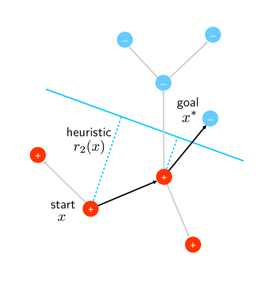
Figure 1: An admissible heuristic for graph search. Circles represent feasible examples ${\mathbb{X}}$, with ${\mathbb{X}}\subset{\mathbb{S}}={\mathbb{R}}^{2}$ being a subset of 2-dimensional Euclidean space. The color and a plus or minus shows the true class of an example. Arrows represent transformations in ${\mathcal{G}}$, with the length of the arrow being the $\mathcal{L}_{2}$ cost of the transformation. Pointwise robustness $r_{2}({\bm{x}})$ over ${\mathbb{S}}$ is the $\mathcal{L}_{2}$ distance from point ${\bm{x}}$ to the decision boundary defined by the target model $f({\bm{x}})={\bm{w}}\cdot{\bm{x}}+b$. The value of an admissible heuristic is $r_{2}({\bm{x}})$ for all ${\bm{x}}$ not classified as target class ($-$), and zero for the other ones.

III-B Computing the Heuristic

III-B1 Linear Models

The MAC $r({\bm{x}})$ over a continuous ${\mathbb{R}}^{m}$ is equivalent to the standard notion of pointwise adversarial robustness, and can be computed efficiently for linear models.

When the target model is a linear model, $\phi({\bm{x}})={\bm{x}}$, $r({\bm{x}})$ is a distance from ${\bm{x}}$ to the hyperplane defined by the discriminant function (see Figure 1), and has a closed form:

$$r({\bm{x}})=\frac{|{\bm{w}}\cdot{\bm{x}}+b|}{\left\lVert{\bm{w}}\right\rVert^{*}}=\frac{|f({\bm{x}})|}{\left\lVert{\bm{w}}\right\rVert^{*}},$$ (7)

where $\left\lVert{\bm{w}}\right\rVert^{*}$ is the dual norm corresponding to $\left\lVert{\bm{w}}\right\rVert$ [44, 45]. If the edge cost is induced by an $\mathcal{L}_{p}$ norm, $\omega({\bm{a}},{\bm{b}})=\left\lVert{\bm{a}}-{\bm{b}}\right\rVert_{p}$, the denominator $\left\lVert{\bm{w}}\right\rVert^{*}$ is $\left\lVert{\bm{w}}\right\rVert_{q}$, where $q$ is the Hölder conjugate of $p$: $\frac{1}{p}+\frac{1}{q}=1$.

III-B2 Non-Linear Models

For some models, $r({\bm{x}})$ can be either computed using formal methods [46, 9, 8], or bounded analytically, yielding a lower bound $\eta({\bm{x}})$ [13, 47, 10]. Existing methods usually perform the computation over a box-constrained ${\mathbb{S}}=I_{1}\times I_{2}\times\cdots\times I_{m}$ for some contiguous intervals $I_{j}\subset{\mathbb{R}}$, and are only applicable to $\mathcal{L}_{p}$ norm-based costs. These methods are much more expensive to compute than the closed-form solution for linear models above.

III-B3 Bounded Relaxations

A number of works explore bounded relaxations of the admissibility properties of A^∗ search, aiming to trade off admissibility guarantees for computational efficiency [41, 48, 49, 50]. In this paper, we employ static weighting [41] for its simplicity. In this approach, the heuristic value is multiplied by $\varepsilon>1$. This results in adversarial examples that have at most $\varepsilon$ times higher cost than MAC.

IV Experimental Evaluation

We evaluate the graph search approach for finding adversarial examples as means to evaluate the security of an ML model by computing its robustness against adversarial examples, and as means to build efficient defenses against privacy-invasive ML models. We use two ML applications that work with constrained discrete domains: a bot detector in a white-box setting, where it is possible to use A^∗ with admissible heuristics to obtain provably minimal-cost adversarial examples, and a traffic-analysis ML classifier in a black-box setting, where we obtain upper bounds on the minimal adversarial cost.

Implementation

We use scikit-learn [51] for training and evaluation of ML models, and Jupyter notebooks [52] for visualizations. The reported runtimes come from executions on a machine with Intel i7-7700 CPU working at 3.60GHz. The code to run the attacks is available as a Python package; all experiments are reproducible.

IV-A Evaluating Security: Twitter-Bot Detection

In this section, we evaluate the security of an ML-based Twitter-bot detector. First, we show how to use the graphical framework to compute adversarial robustness as the minimal cost of building a bot that can evade detection, and compare the guarantees the framework provides to the standard adversarial robustness measures. Second, we evaluate the efficiency and optimality of our attacks. At the end of this section, we discuss the implications of our assumptions when the framework is used as a security evaluation tool.

As in our toy example, we assume the adversary starts with a bot account and aims to find the minimum transformation that make the model classify the account as human. They define a transformation graph such that any chain of transformations results in a feasible account, runs the graph search to find a minimal-cost example, and replicates the transformations on their bot account to evade the classifier.

Note that, as opposed to adversarial examples on images where the perturbations added by the adversary may change the content of the image to the point where it changes its class, in our setting, a bot account will keep being a bot account regardless of the transformations.

IV-A1 Twitter-Bot Detector

We use a linear model as the target classifier that classifies an account as a “bot” or “not bot”. In particular, we use $\mathcal{L}_{2}$-regularized logistic regression, as the use of a linear model enables us to compute the exact value of the heuristic efficiently (see Section III-B). The decision threshold of the classifier is standard: $d=0.5$. We use 5-fold cross-validation on the training set (see below) to pick the $\mathcal{L}_{2}$ regularization parameter of the logistic regression (set to $1.9$). Although simple, this classifier yields an accuracy of 88% (random baseline is 65%) and performs on par with an SVM with an RBF kernel, and better than some neural network architectures (see Section IV-A4). Hence, we consider the regression to be a realistic choice in our setting.

Dataset

We use the dataset for Twitter bot classification by Gilani et al. [54]. Each example in this dataset represents aggregated information about a Twitter account in April of 2016. Concretely, it has the following features: the number of tweets, retweets, favourites, lists, and replies, the average number of URLs, the size of attached content, average likes and retweets per tweet, and the list of apps that were used to post tweets (see Table II).

Accounts are human-labeled as bots or humans. The original dataset is split into several bands by the number of followers. We report the results for the 1,289 accounts with under 1,000 followers; more popular accounts result in similar behavior. We randomly split the dataset into training and test sets, containing 1160 and 129 accounts or, respectively, 90% and 10% samples. We generate adversarial examples for the 41 accounts in the test set that are classified as bots by the target classifier.

TABLE II: Features from the Twitter bot classification dataset by Gilani et al. [54]

Feature	Column name	Type
Number of tweets	user_tweeted	Integer
Number of retweets	user_retweeted	Integer
Number of replies	user_replied	Integer
Age of account, days	age_of_account_in_days	Integer
Total number of URLs in tweets	urls_count	Integer
Number of favourites (normalized)	user_favourited	Float
Number of lists (normalized)	lists_per_user	Float
Average number of likes per tweet	likes_per_tweet	Float
Average number of retweets per tweet	retweets_per_tweet	Float
Size of CDN content, kB	cdn_content_in_kb	Float
Apps used to post the tweets	source_identity	Set
Total number of apps used	sources_count	Integer
Followers-to-friends ratio†	follower_friend_ratio	Float
Favourites-to-tweets ratio†	favourite_tweet_ratio	Float
Average cumulative tweet frequency†	tweet_frequency	Float

$\dagger$ We have dropped this feature from the dataset, since the effect of transformations on it cannot be computed without having original tweets. We were not able to obtain the original dataset of the tweets for compliance reasons.

Feature Processing

Almost all the features in the dataset are numeric (e.g., size of attached content). We use quantile-based bucketization to distribute them into buckets that correspond to quantiles in the training dataset. In our experiments, we use 20 buckets, which offers best performance in a grid search measuring 5-fold cross-validation accuracy on the training set. After bucketization, we one-hot encode the features.

The only non-numerical feature is the list of apps that were used to post the tweets. We encode it as follows. For each of the six apps in the dataset, we use two bits: if the app was used by the account we set the first bit, and if not, we set the second bit.

IV-A2 Security Evaluation

Here, we evaluate the security of the bot detector using minimal adversarial costs as the measure of adversarial robustness.

The Adversary’s Goals

As mentioned in Section II-B1, the minimal adversarial costs depend on the adversary’s definition of “fooling”. To illustrate how the framework can accommodate different goals, we simulate two attack settings. First, a basic attack, in which the adversary’s goal is to find any adversarial examples that flip the decision of the classifier ($l=d=0.5$). Second, a high-confidence attack, in which the adversary’s goal is to find adversarial examples that are classified as “not bot” with at least 75% confidence ($l=0.75$).

The Adversary’s Capabilities: Transformation Graph and Cost

For this evaluation, we assume that the adversary is capable of changing all account features, and the cost of an adversarial example is the number of changes required to transform an initial bot account into that example. This adversarial cost model is similar to the state of the art in adversarial ML (see Section V-A). In Section IV-A4, we discuss a different model in which the adversary is constrained by the number of features that they can influence, and the cost is not measured in the number of changes, but in the actual dollar cost of performing transformations.

We build the transformation graph by defining atomic transformations that change only one feature value. For each bucketed feature we define two atomic transformations: increasing the feature value so that it moves one bucket up, and decreasing the feature value so that it moves one bucket down. For the buckets in the extremes, only one transformation is possible. For the list of apps feature, we define one transformation per app: flipping the bits that represent whether the app was used or not. Then, all possible modifications of an initial example, including those that change multiple features, can be represented as chains of atomic transformations: paths in the graph. For example, a modification that changes two features needs at least two atomic transformations: a path with two edges.

We define the edge costs to be the $\mathcal{L}_{1}$ distance between feature vectors before and after a transformation. Given the one-hot encoding, this means that each atomic transformation in our graph has a constant cost of 2 (one bit is set to zero, and another bit to one). Such a representation has two advantages. First, the path cost can be easily related to the number of changes needed to evade the classifier: it suffices to divide the path cost by two. Second, because the edge cost is a norm-induced metric, we can use A^∗ with admissible heuristic by Statement III.1. Figure 2 illustrates an example transformation graph for simplified accounts.

Note that the $\mathcal{L}_{1}$ distance between two arbitrary feature vectors does not represent the number of changes between them. We are able to represent the number of changes through the structure of the transformation graph.

Figure 2: Sketch of the transformation graph for simplified Twitter accounts. Italics denote a feature value that differs from the initial example. The edge costs are constant and equal to the $\mathcal{L}_{1}$ distance between the feature vectors representing the accounts.

Results

We run A^∗ search on the transformation graph to find adversarial examples. For the basic attack, i.e., when the adversary wants to find an example that flips the decision regardless of the confidence, on average only 2.2 (s.d. 1.6) feature changes suffice to flip the decision of the target model. To obtain adversarial examples with high confidence ($75\%$), the adversary needs on average 3.9 (s.d. 2.7) changes. We report some examples of adversarial example accounts in Table VI (Appendix C).

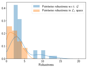
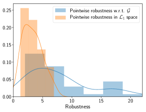
Figure 3: Pointwise adversarial robustness measured as minimal-cost adversarial examples computed using the transformation graph ${\mathcal{G}}$, and pointwise robustness in $\mathcal{L}_{1}$ space. Left: basic attack. Right: high-confidence attack. (Notice the different y-axes)

Next, we compare the minimal adversarial cost of adversarial examples as a security measure to the standard notion of adversarial robustness over continuous ${\mathbb{S}}={\mathbb{R}}^{m}$ (as in Equation 5). We show in Figure 3 the distribution of the values of both measures for the basic and high-confidence attacks. We see that the MAC values from our method are up to 26$\times$ higher than adversarial robustness over the unconstrained $\mathcal{L}_{1}$ space in the case of the basic attack, and up to 486$\times$ higher in the case of the high-confidence attack.

This means that the continuous domain robustness measure applied to a discrete domain results in overly pessimistic adversarial cost estimates, that an adversary cannot achieve because of inherent domain constraints. Our approach produces a more precise robustness measure, tailored to the concrete domain constraints and the adversary’s capabilities.

IV-A3 Performance Evaluation

Here, we study the trade-off between being able to run the graph search efficiently and the optimality guarantees of the obtained MAC values. We consider the following algorithms: uniform-cost search (UCS), plain A^∗, and $\varepsilon$-bounded relaxations of A^∗ with $\varepsilon=\{2,3,5,10\}$ (see Section III-B3).

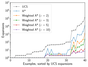
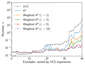
Figure 4: Basic attack performance performance. Left: node expansions. Right: runtime in seconds. (y-axes are logarithmic)

Runtime

Figure 4 shows the number of expansions (left), as well as the runtime (right), needed to find adversarial examples that flip the detector in the basic attack. We find that A^∗ expands significantly fewer nodes than UCS (up to 32$\times$ fewer), showing that our admissible heuristic is indeed useful for efficiently finding MAC adversarial examples in the search space. Relaxing the optimality requirement by increasing the $\varepsilon$ weight speeds up the search even more. For instance, $\varepsilon=5$ decreases runtime by three orders of magnitude, and still ensures that the minimal cost is at most five times lower than the cost of the found adversarial example. We also observe that in some cases UCS performs better than A^∗ in terms of the runtime, even though A^∗ expands fewer nodes. We believe that this is an artifact of our Python implementation, which could be solved with a more efficient implementation.

We observe similar results for the high-confidence attack (Figure 5). High-confidence adversarial examples require more transformations, hence, the search takes up to 100$\times$ more runtime than for the basic attack. Still, A^∗ performs significantly better than UCS, expanding 2–31$\times$ fewer nodes.

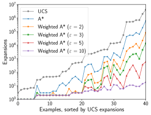
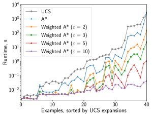
Figure 5: High-confidence attack performance. Left: node expansions. Right: runtime in seconds. (y-axes are logarithmic)

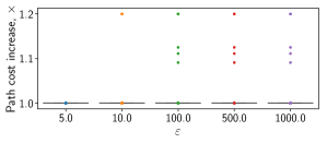
Figure 6: High-confidence attack: increase in cost over MAC of adversarial examples found using $\varepsilon$-weighted A^∗.

Speed vs. Optimality Trade-Off

We saw that $\varepsilon$-bounded relaxations can drastically decrase the search runtime. We empirically assess by how much this speedup hurts the optimality of obtained adversarial examples. To evaluate this, we compute the increase in costs of adversarial examples found with $\varepsilon$-weighted A^∗ over the optimal adversarial examples found with plain A^∗. We discover that the upper bound on sub-optimality from $\varepsilon$-weighted A^∗ is extremely pessimistic (recall that $\varepsilon$-weighting guarantees that the found adversarial examples have at most $\varepsilon$ times higher cost than the MAC). In practice, for the tested values of $\varepsilon$, all adversarial examples found in the basic attack incur minimal cost in our transformation graph, and only few high-confidence adversarial examples have costs at most $1.2\times$ higher than the MAC (see Figure 6). We conclude that for this setting, using $\varepsilon$-weighting can bring huge performance benefits at no cost.

Heuristics Comparison

Up to this point, we used $\mathcal{L}_{1}$ distance as an edge weight, and the corresponding $\mathcal{L}_{1}$-based heuristic in the search. Here, we investigate if other heuristics provide better performance. To maintain the optimality of A^∗, the edge weights have to change accordingly. Given that we consider that all transformations have the same cost, a uniform change in the weights results in an equivalent transformation graph. The difference lies in the multiplicative factor used to recover the number of required changes from the path cost.

We run the basic attack using $\mathcal{L}_{1}$, $\mathcal{L}_{2}$, and $\mathcal{L}_{\infty}$ edge weights, i.e., 2 for $\mathcal{L}_{1}$, $\sqrt{2}$ for $\mathcal{L}_{2}$, and $1$ for $\mathcal{L}_{\infty}$; and the corresponding heuristics, that we denote as $r_{1},r_{2},r_{\infty}$. We compare the performance of A^∗ for these edge costs against each other and against two baselines. First, UCS, which expands the same number of graph nodes for all three edge cost models. It represents the worst case in terms of performance, but outputs provably minimal-cost adversarial examples. Second, we run “random search” 10 times. By random search we mean A^∗ with a heuristic that outputs random numbers between 0 and 2 on the transformation graph with $\mathcal{L}_{1}$ edge costs. This algorithm is efficient, but does not provide any optimality guarantees.

We show the result in Figure 7 (left). Except for adversarial examples that lie deeper in the graph, all admissible heuristics find solutions faster than the random search. We also see that the random search outputs adversarial examples that have costs up to 11 times the MAC obtained with A^∗.

Even though both $\mathcal{L}_{2}$ and $\mathcal{L}_{\infty}$ heuristics enable the algorithm to explore fewer graph nodes than UCS, in practice they take the same time (see Figure 7, right) This is because each heuristic exploration is quite costly in terms of computation time. The edge weights for $\mathcal{L}_{2}$ and $\mathcal{L}_{\infty}$ ($\sqrt{2}$ and $1$, respectively) are comparatively high compared to the values of the heuristics (on our dataset $r_{2}$ is on average 0.52 and $r_{\infty}$ is on average 0.059). Hence, A^∗ often needs to explore all nodes of the same cost before it can proceed to transformations that carry a higher cost, essentially degenerating into UCS. On the contrary, $\mathcal{L}_{1}$ heuristics perform consistently better, as $r_{1}$ is on average 2.18, higher than 2 (the $\mathcal{L}_{1}$ edge cost). We note that this result may not necessarily hold for other transformation graphs with different cost models.

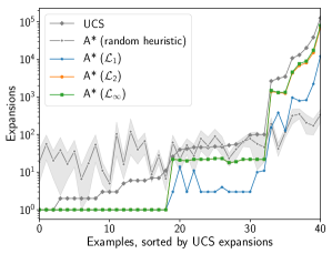
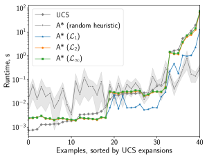
Figure 7: Basic attack heuristics comparison. Left: node expansions. Right: runtime in seconds. (y-axes are logarithmic)

IV-A4 Applicability Discussion

In the previous experiments, we assumed that the target model is linear, that the adversarial cost is proportional to the number of feature changes, and that the adversary has white-box knowledge and uses optimal algorithms. In this section, we explore other options for each of these assumptions and, in Section IV-B, we conduct a thorough evaluation of a setting in which none of them hold.

Non-Linear Models

When the target model is linear, we can efficiently compute the exact value of the the admissible heuristic from Equation 6. Even though a linear model is a sensible choice in our setting, non-linear models can often appear in other security-critical settings. Mounting an A^∗-based attack against a non-linear target model, however, requires costly methods to compute the heuristic (see Section III-B).

One way to overcome this issue is linearizing the non-linear model using a first-order Taylor expansion, and then using the heuristic $r$ for linear models (see Appendix B for a formal derivation):

$$r({\bm{x}})\approx\frac{|f({\bm{x}})|}{\left\lVert\nabla_{{\bm{x}}}f({\bm{x}})\right\rVert^{*}}$$ (8)

We note that, as this approximation can overestimate $r({\bm{x}})$, it cannot serve as an admissible heuristic without additional assumptions on $f$.

We empirically evaluate this heuristic by running the attack against an SVM with the RBF kernel trained on the dataset with discretization parameter set to 20 (88% accuracy on the test set). Using UCS to obtain the ground-truth minimal-cost adversarial examples, we find that, even though the heuristic is approximate, all adversarial examples found with A^∗ are minimal-cost. Moreover, this heuristic allows the graph search to use significantly fewer graph node expansions than UCS (Figure 8, left). On the downside, even though the algorithm expands fewer nodes, the overhead of computing the heuristic (which includes computing the forward gradient of the SVM-RBF) is high enough that there is no actual improvement in performance, unless we use $\varepsilon>2$ weighting (Figure 8, right). More efficient implementations of the heuristic can result in better gains.

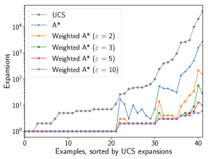
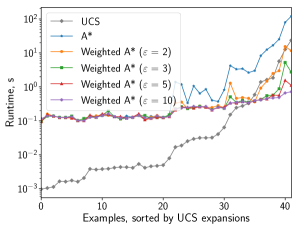
Figure 8: Basic attack against a non-linear model (SVM-RBF) using an approximate heuristic. Left: node expansions. Right: runtime in seconds. (y-axes are logarithmic)

TABLE III: Transferability of minimal-cost adversarial examples from logistic regression to other models. Columns: model; Accuracy—model’s accuracy on the test set; Trans. (basic)—transferability rate of adv. examples aiming to be missclassified with 50% confidence to this model; Trans. (high)—same, with 75% confidence.

Model	Accuracy, %	Trans. (basic), %	Trans. (high), %
LR	88	—	—
NN-A	80	49	84
NN-B	83	38	95
GBDT	87	74	95
SVM-RBF	88	73	100

Black-Box Setting

The minimal-cost adversarial examples, and the robustness guarantees they induce, are specific to a particular target model. Do other models misclassify these examples as well? If yes, the attack would not only be effective in the white-box setting, but also in the black-box setting, where the adversary does not know the exact architecture and weights of the target model. Furthermore, there would be no need to use expensive heuristics for non-linear models.

We check whether the adversarial examples found in the previous section using A^∗ against a logistic regression (LR) are misclassified by other non-linear models trained on the same dataset. We choose four ML models representative of typical architectures: two instantiations of a two-layer fully-connected ReLU neural network, one with 2000 and 500 neurons (NN-A), and one with 20 and 10 neurons in the respective layers (NN-B); gradient-boosted decision tree (GBDT); and an SVM-RBF. We do not run extensive hyperparameter search to obtain the best possible performance of these models, but we ensure that all of them have accuracy greater than $80\%$ (the random baseline is $65\%$).

Table III shows the results of the experiment. We see that the basic minimal-cost adversarial examples (which mostly have confidence only slightly higher than 50%) transfer to the other models in at least 38% of the cases and in about 73% of the cases for GBDT and SVM-RBF. In the high-confidence setting more than 83% of the adversarial examples transfer to all models. We conjecture that when the goal is to find any adversarial examples, the minimal-cost adversarial examples often exploit a weakness found only in their target model, and, hence, rarely transfer. When the target confidence level is higher, the adversarial examples require more transformations and become similar to non-bots as seen in the training data. Hence, they are more likely to generalize.

Non-Optimal Algorithms

So far we have considered that the adversary uses algorithms that provide optimality guarantees: UCS, A^∗, $\varepsilon$-weighted A^∗. These algorithms are often expensive. We investigate the performance of less expensive non-optimal algorithms in our setting using a hill-climbing modification of A^∗ as an example (see Section II-A2). Regular A^∗ needs to keep track of all previously expanded nodes at any given time. The hill-climbing variation only keeps the best-scoring node. This significantly improves memory and computation requirements, but sacrifices the ability of A^∗ to backtrack.

We see in Figure 9 that hill climbing performs significantly better than UCS and A^∗. Furthermore, we find that, in the basic-attack setting, all adversarial examples found by the hill climbing incur minimal cost; and in the high-confidence setting only some are more expensive (at most $1.2\times$ higher than the minimal cost). We note that these results are on par with weighted A^∗ for $\varepsilon=10$, with the difference that hill climbing does not provide any provable guarantees.

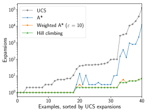
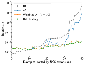
Figure 9: Basic attack setting comparison of UCS, A^∗, weighted A^∗, and hill climbing. Left: node expansions. Right: runtime in seconds. (y-axes are logarithmic)

Realistic Adversarial Costs

Previously, we ensured that the chosen edge weights allow to use admissible heuristics in A^∗, and assumed that the adversary can modify all features at the same cost. However, the general graphical framework and, more importantly, the problems it represents in practice, are not limited to these transformation costs or such a powerful adversary.

Here, we show how the graphical approach can accommodate a more realistic scenario. We constrain the transformation graph to modify only the features that can be changed with the help of online services. As of this writing, there exist online services that charge approximately $2 for ghost-writing a tweet or a reply; and services that charge approximately $0.025 for a retweet or a like of a given tweet. Hence, we constrain the adversary to modify only the number of tweets, the number of replies, the likes per tweet, and the retweets per tweet features. Moreover, we constrain the adversary to only increase the value of any transformable feature (e.g., we assume the adversary can hire someone to write more tweets, but not to delete them).

We set the weights of the edges such that they correspond to the dollar costs of the atomic transformations. This cost is estimated as follows. We compute the difference between the previous value of the feature and the lowest endpoint of the bucket in which the new feature value ends up. We then multiply this difference (the number of tweets, replies, incoming likes, or incoming retweets that need to be created or added) by the respective price in the mentioned online services. As a result, path costs in such a graph are lower bounds on the dollar cost the adversary has to pay to perform a sequence of transformations. Hence, these costs can be used to make informed risk analysis regarding the security of a model.

Table IV shows the results of running UCS to obtain MAC values for the basic and high-confidence attacks on this transformation graph. Because of the restricted transformations, we can find adversarial examples only for 70% and 19% of the initial examples, for the basic and the high-confidence setting, respectively. In particular, we observe that if an initial example is classified as “bot” with high enough confidence (approximately 80% for the basic attack), it is unlikely that we can find a corresponding adversarial example.

Even though for simplicity we used UCS, the edge weights could be expressed as a weighted norm, e.g., $\left\lVert A({\bm{x}}-{\bm{x}}^{\prime})\right\rVert_{1}$ for some positive-definite weight matrix $A$ encoding the costs of the transformations. This means that it is possible to derive an admissible heuristic and employ A^∗. We leave the derivation of such heuristic as an open line of research.

TABLE IV: Dollar cost of adversarial examples against bot detection. Columns: Attack—attack setting: required confidence level for adversarial examples; Exists—proportion of initial examples for which an adversarial example exists; Minimal adversarial cost—minimum, average, and maximum values of minimal adversarial costs for the part of the test dataset for which adversarial examples exist.

		Minimal adversarial cost
Attack	Exists	min.	avg.	max.
Basic (50%)	70%	$0.02	$35.7	$281.6
High (75%)	19%	$3.8	$57.6	$218.2

IV-B Building Defenses: Website Fingerprinting

In the previous section, we considered a setting in which the adversary’s knowledge is white-box. This assumption, however, does not always hold in practice. When the access to the ML model is black-box, the adversary cannot use the admissible heuristic to efficiently obtain minimal-cost adversarial examples using A^∗. We show that even in this setting the graphical framework is a useful tool for finding adversarial examples in constrained domains.

In this section, we also change the adversarial perspective. We consider a scenario in which the ML model is at the core of a privacy-invasive system and the entity deploying adversarial examples is a target of this system. Therefore, the model becomes the adversary, and adversarial examples become defenses.

Concretely, we take the case of website fingerprinting (WF), an attack in which a network adversary attempts to infer which website a user is visiting by only looking at encrypted network traffic [31, 32], often using machine learning [33, 55, 56, 57, 58]. This attack is mostly considered a threat to users of anonymous communication networks such as Tor [59]. However, as the encrypted SNI proposal [60] becomes standardized within TLS 1.3 [61]—hiding the destination of encrypted HTTPS traffic from network observers—this attack becomes a privacy threat to all Internet users. To counter the attack, existing ad-hoc defenses transform the traffic to reduce the accuracy of the ML classifier [33, 34, 35, 36, 37].

We first show how the graphical framework can be used as a systematic tool for designing traffic modifications that defend users against a WF adversary. We then show how the defenses produced by our method can be used as a baseline to evaluate both the effectiveness (ability to fool a classifier) and efficiency (incurred overhead) of existing defenses.

IV-B1 Website-Fingerprinting Attack

We consider a WF adversary that takes as input a network trace, i.e., a sequence of incoming (from server to client) and outgoing (from client to server) encrypted packets, and outputs a binary guess of whether the user is visiting a website that is in the monitored set or not. For instance, this could be a censorship adversary that wants to know if the visited website is in a list of censored websites in order to stop the connection.

We simulate a WF adversary that uses the classifier by Panchenko et al. [33], an SVM with an RBF kernel trained on CUMUL features. For a given trace, a CUMUL feature vector contains the total incoming and outgoing packet counts, and 100 interpolated cumulative packet counts. We refer the reader to the original paper for the details on computing the vector.

Dataset

We use the dataset of Tor network traces collected by Wang et al. [55]. This dataset contains 18,004 traces, half of them coming from a simulated monitored set compiled from 90 websites censored in China, the UK, and Saudi Arabia, and half coming from a non-monitored set of 5,000 other popular websites. The average trace length is 2,155.

We randomly split the dataset into 90% training and 10% testing subsets of 15,397 and 1,711 traces, respectively. We use these splits to train and test the target WF classifier. To keep the running time of our experiments reasonable, we find adversarial examples only for traces with less than 2000 packets that are classified as being in the monitored set. There are 577 such traces, with an average length of 1750 packets.

The CUMUL classifier performs remarkably well on our test dataset, with an accuracy of 97.8% (the random baseline is 50%). Thus, we consider it is a good example to illustrate the potential of our framework.

IV-B2 Building Defenses

The Defender’s Goals

The goal of the defender is to modify monitored traces such that they are misclassified as non-monitored by the WF classifier. These modifications can be of two kinds: adding dummy packets and adding delay. Removing packets is not possible without affecting the content of the page, and the delay is dependent on the network and cannot be decreased from an endpoint. The previous work (e.g., Panchenko et al. [33]) has noted that perturbing timing information is not as important to classification as the volume of packets. Hence, even though adding delay is possible within the graphical framework, we consider that our defense only adds dummy packets. As in the previous works, we assume that dummy packets are filtered by the client and the server and do not affect the application layer.

Adding dummy packets has a cost in terms of bandwidth and delay (routers have to process more packets). Therefore, the defender wants to introduce as few packets as possible. In terms of confidence level $l$, we consider only the case where the defender wants to flip the classifier decision ($l=d=0.5$). Finding higher confidence adversarial examples is possible at the cost of running a longer search.

The Defender’s Capabilities: Transformation Graph and Cost

For a given trace we define the following transformations: add one dummy outgoing packet, or one dummy incoming packet, between any two existing packets in the trace. This means that each node in the transformation graph is a copy of its parent trace with an added dummy packet. We assign every transformation a cost equal to one, thus representing the added packet. Path costs in this graph are equal to the number of added packets.

Heuristic and Search Algorithms

Recall that CUMUL feature processing includes an interpolation step. Because of the interpolation part of a CUMUL feature vector, the costs in our transformation graph can not be trivially expressed as norm-induced distances between the feature vectors. Hence, we cannot use the admissible heuristic from Equation 6, or its approximated version. Instead, we use the following confidence-based heuristic, similar to the heuristics used in other attacks in discrete domains (e.g., by Gao et al. [22]):

$$h_{t}(x)=\begin{cases}+f(x),&t=0\\ -f(x),&t=1\\ -\infty,&F(x)=t\\ \end{cases}$$

The value of this heuristic becomes lower as the confidence of the WF classifier for the target class (non-monitored in our case) becomes higher. Note that this heuristic does not require any knowledge of the classifier, only the ability to query $f(x)$.

As in this case we cannot use optimal algorithms, we implement the hill climbing variation of the greedy best-first search ($\mathsf{score}(x)=h(x)$ for its speed, see Section II-A2). We also limit the number of iterations of the algorithm to 5,000 in order to keep down the runtime of our experiments. Our results show that this is sufficient to find adversarial examples in 100% of the cases.

We also run a random search, i.e., we follow a random path in the graph until an adversarial example is found, to obtain a baseline in terms of cost and runtime. We run this algorithm three times for each trace with different random seeds.

Results

Hill climbing with the confidence-based heuristic finds adversarial traces in 100% of the cases, with an average time to find an adversarial example of 0.8 seconds. Random search succeeds in slightly less than 100%, with an average time of about 0.3 seconds. As we discuss below, the results differ in the overhead required to find an adversarial example.

IV-B3 Comparing Defenses

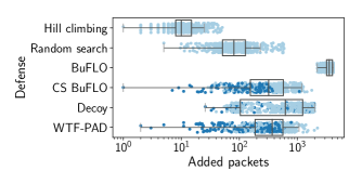
Figure 10: Left: number of added packets by WF defenses and adversarial examples (x-axis is logarithmic). Center: overhead of WF defenses compared to the number of packets added by adversarial examples found with hill climbing (x-axis is bi-symmetrically logarithmic). Right: success rates of WF defenses and adversarial examples against the SVM-RBF classifier.

Here, we use minimal-cost adversarial examples for website fingerprinting to evaluate existing ad-hoc WF defenses: Decoy pages [33], BuFLO [34], CS BuFLO [36], and adaptive padding (WTF-PAD) [37]. We use the implementations of Decoy pages and BuFLO by Wang, CS BuFLO by Cherubin [62], and WTF-PAD by Juárez et al. [37]. Concretely, we measure the overhead in terms of (1) the number of dummy packets added, and (2) the success rates of the defenses, i.e., the percentage of traces for which they successfully evade the classifier.

We evaluate the efficiency by measuring the raw overhead in terms of added packets (see Figure 10, left). The existing defenses add up to 3000 dummy packets. Unexpectedly, BuFLO, which is deliberately inefficient, is the most expensive defense. On the contrary, adversarial examples add on average 12 dummy packets, and at most 52.

In terms of relative overhead, i.e., how many more packets the defenses add, compared to the adversarial examples found using hill climbing, all defenses and random search require significantly more bandwidth (see Figure 10, center). In five cases, CS BuFLO and WTF-PAD add fewer packets, but in those cases the defenses do not succeed in evading the classifier.

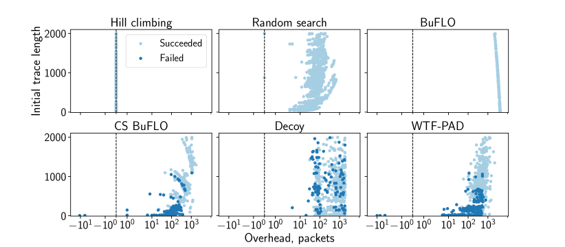
Figure 11: Overhead of WF defenses compared to adversarial examples found with hill-climbing search (x-axis is bi-symmetrically logarithmic)

We then analyze the defenses’ success rates in the light of the overhead they impose. The graph search yields a 100% success rate, whereas the existing defenses (aside from BuFLO) only succeed in 70%—80% of the cases (Figure 10, right). Also, as it can be seen in Figure 10 (center), increasing the number of packets is not a guarantee of success. We see how for all defenses but BuFLO some cases fail even with hundreds of overhead packets. A closer analysis shows that CS BuFLO and WTF-PAD often fail to defend shorter traces (under 1000 packets), whereas they can successfully defend the longer ones (see Figure 11 in Appendix C for illustration).

This hints that the ad-hoc defenses use the dummies in an inefficient way, and there is a significant room for improvement. The adversarial examples found with hill climbing present a tight upper bound on the minimal cost of any successful defense. Hence, we hope that our graphical framework can serve as a baseline to evaluate the efficiency of future defenses, and guide the design of effective website-fingerprinting countermeasures.

IV-B4 Applicability Discussion

In this section, we apply the graphical framework to a setting with no white-box knowledge, against a non-linear classifier, by using non-optimal algorithms, and show that the framework is still useful when none of the assumptions from Section IV-A hold.

We do not evaluate the transferability of obtained adversarial examples to other classifiers. The main reason is that the state-of-the-art WF classifiers are based on deep learning [58, 57], thus require datasets larger than the one we use in our comparison. Although we leave the transferability evaluation for future work, we expect that the results would be qualitatively similar to those in the Twitter-bot case (see Section IV-A4).

V Related Work

We overview existing attacks in discrete domains and highlight their differences with respect to our work.

Discretized Image Domain

Papernot et al. propose the Jacobian saliency map approach (JSMA) [4] to find adversarial images. JSMA is a greedy white-box attack that transforms images by increasing or decreasing pixel intensity to maximize saliency, that is computed using the forward gradient of the target model. This attack is a basis for attacks in other discrete domains [20, 16], as we discuss below.

Text Domain

Multiple works study evasion attacks against text classifiers [63, 24, 19, 21, 64, 22, 15, 65]. Recent attacks can be divided into three groups: those employing a hill-climbing algorithm over the set of possible transformations of an initial piece of text [19, 21, 64, 22]; those that greedily optimize the forward gradient-based heuristic but run beam search [15]; and those that use an evolutionary algorithm [65].

Malware Domain

Several works explore evasion attacks for malware, either adapting JSMA [20], applying forward gradient-based heuristics [17], using a black-box hill-climbing algorithm over a set of feasible transformations [66], or using a black-box evolutionary algorithm [67].

Protecting Users

Finally, some works use adversarial examples as means to protect users. Jia and Gong adapt JSMA to modify user-item relationship vectors in the context of recommendation systems. Overdorf et al. use exhaustive search to find adversarial examples that counter anti-social effects of machine learning.

V-A Comparison to Our Work

Our framework can be seen as a generalization of most of the attacks mentioned previously. Moreover, it can encode arbitrary adversarial costs, and can be configured to output minimal-cost adversarial examples using A^∗ search. We note that in parallel to our work, Wu et al. also used A^∗ and randomized tree search to obtain bounds on robustness of neural networks [68]. Their work, however, only considers the setting of image recognition.

Dalvi et al. [63] have used integer linear programming to find approximate minimal-cost adversarial examples against a Naïve Bayes classifier. Our graphical framework enables us to consider arbitrary transformations and cost models and to find minimal-cost adversarial examples for any non-linear classifier for which adversarial robustness in a continuous domain can be computed.

Except for the method by Dalvi et al. and the attacks based on evolutionary algorithms, all of the attacks above can be instantiated in our graphical framework (see Table V in Appendix C for a summary of such instantiations). The attacks implicitly define a transformation graph by specifying a set of domain-specific transformations (e.g., word insertions for text) that define the graph. The cost of transformations can be equal to the number of such transformations (e.g., [19, 21]), or, equivalently, to the $\mathcal{L}_{p}$ distance between feature vectors interpreted as the number of transformations (e.g., [20, 16]).

The attacks can be seen as special cases of running the BF^∗ search algorithm (see Section II-A2) over a transformation graph. They differ in adversarial knowledge assumptions (white-box or black-box), transformation graphs, adversarial cost models, and the choice of the scoring function and priority-queue capacity that defines the instantiation of BF^∗.

Most of the attacks (e.g., [19, 21, 20, 16]) run a hill-climbing search over the transformation graph. They maximize a heuristic either based on the forward gradient of the model (in the white-box setting where the adversary can compute the gradient), or on the confidence (in the black-box setting where the adversary can only query the model). Ebrahimi et al. [15] use beam search instead of hill climbing, Kulynych [69] uses an instance of backtracking best-first search, and Overdorf et al. [23] use an exhaustive search over the space of feasible transformations, equivalent to UCS.

VI Conclusions

In this paper, we proposed a graphical framework for formalizing evasion attacks in discrete domains. This framework casts attacks as search over a graph of valid transformations of an initial example. It generalizes many proposed attacks in various discrete domains, and offers additional benefits.

First, as a formalization, it enables us to define arbitrary adversarial costs and to choose search algorithms from the vast literature on graph search, whereas the previous attacks often use $\mathcal{L}_{p}$ norms as costs and mostly focus on hill-climbing strategies.

Second, we show that when it is possible to compute adversarial robustness in a continuous domain, this robustness measure can be used as a heuristic to efficiently explore a discrete domain. Thus, an adversary with the white-box knowledge can use A^∗ search to obtain adversarial examples that incur minimal adversarial cost. This enables us to provably evaluate the adversarial robustness of a classifier given the domain constraints and adversary’s capabilities.

Third, the versatility of our framework to model transformations and their costs independently of the ML model under attack make it suitable to tackle both security and privacy problems. As examples, we showed how it can be used to evaluate the adversarial robustness of a Twitter-bot classifier, and to evaluate the cost-effectiveness of privacy defenses against a website-fingerprinting classifier.

Appendix A Proof of Statement III.1

Observe that if $F({\bm{x}})=t$, the heuristic $r({\bm{x}})=0$, and hence is trivially admissible. Indeed, it cannot overestimate $C_{{\mathcal{G}}}({\bm{x}},{\bm{x}}^{*})$ due to the fact that $\omega(a,b)\geq 0$ and $C_{{\mathcal{G}}}(a,b)\geq 0$ for any $a,b\in V$.

It is therefore sufficient to show that if $F({\bm{x}})\neq t$, the lower bound on adversarial robustness at $x$ over ${\mathbb{S}}$ never overestimates $C_{{\mathcal{G}}}({\bm{x}},{\bm{x}}^{*})$:

$$\eta({\bm{x}}^{\prime})\leq C_{{\mathcal{G}}}({\bm{x}},{\bm{x}}^{*})$$ (9)

The following sequence holds:

$$r({\bm{x}}) \leq\left\lVert{\bm{x}}-{\bm{x}}^{*}\right\rVert$$

$$\leq C_{{\mathcal{G}}}({\bm{x}},{\bm{x}}^{*})$$

The first inequality is by definition of $r({\bm{x}})$ (see Equation 5). Indeed, since $r({\bm{x}})$ is a norm of the smallest adversarial perturbation $\Delta$ over ${\mathbb{S}}$, $\Delta$ is smaller than the distance from ${\bm{x}}$ to any other ${\bm{x}}^{\prime}\in{\mathbb{X}}\subseteq{\mathbb{S}}$ that also flips the decision of the target classifier:

$$r({\bm{x}})=\left\lVert\Delta\right\rVert\leq\left\lVert{\bm{x}}-{\bm{x}}^{\prime}\right\rVert\quad\text{\footnotesize(for \emph{any} ${\bm{x}}^{\prime}\in{\mathbb{X}}$ s.t. $F({\bm{x}}^{\prime})=t$)}$$

By Equation 1, $C_{{\mathcal{G}}}({\bm{x}},{\bm{x}}^{*})$ is a path cost for some path:

$$C_{{\mathcal{G}}}({\bm{x}},{\bm{x}}^{*}) =W({\bm{x}}\rightarrow{\bm{v}}_{1}\rightarrow\ldots\rightarrow{\bm{v}}_{n-1}\rightarrow{\bm{x}}^{*})$$

$$=\left\lVert{\bm{x}}-{\bm{v}}_{1}\right\rVert+\sum_{i=1}^{n-2}\left\lVert{\bm{v}}_{i}-{\bm{v}}_{i+1}\right\rVert+\left\lVert{\bm{v}}_{n-1}-{\bm{x}}^{*}\right\rVert$$

By triangle property of the norm, the second inequality holds:

$$\left\lVert{\bm{x}}-{\bm{x}}^{*}\right\rVert \leq\left\lVert{\bm{x}}-{\bm{v}}_{1}\right\rVert+\sum_{i=1}^{n-2}\left\lVert{\bm{v}}_{i}-{\bm{v}}_{i+1}\right\rVert+\left\lVert{\bm{v}}_{n-1}-{\bm{x}}^{*}\right\rVert$$

$$=C_{{\mathcal{G}}}(x,{\bm{x}}^{*})$$

Hence, $r({\bm{x}})\leq C_{{\mathcal{G}}}({\bm{x}},{\bm{x}}^{*})$, which implies Equation 9, and concludes the proof.

Appendix B Derivation of the heuristic approximation for non-linear models

W.l.o.g, assume that the decision threshold of the target classifier is $\theta=0$. For an initial ${\bm{x}}\in{\mathbb{R}}^{m}$, the smallest adversarial perturbation $\Delta\in{\mathbb{R}}^{m}$ puts ${\bm{x}}+\Delta$ on the decision boundary: $f({\bm{x}}+\Delta)=\theta=0$.

Let $\tilde{f}({\bm{x}}+\Delta)$ be the first-order Taylor approximation of $f$ at ${\bm{x}}+\Delta$:

$$\tilde{f}({\bm{x}}+\Delta)=f({\bm{x}})+\nabla_{{\bm{x}}}f({\bm{x}})\cdot\Delta$$

We want to estimate $\Delta$ assuming $\tilde{f}({\bm{x}}+\Delta)=f({\bm{x}}+\Delta)=0$. By Hölder’s inequality,

$$|f({\bm{x}})|=|\nabla_{{\bm{x}}}f({\bm{x}})\cdot\Delta|\leq\left\lVert\nabla_{{\bm{x}}}f({\bm{x}})\right\rVert^{*}\left\lVert\Delta\right\rVert$$

Hence, assuming that $\tilde{f}({\bm{x}}+\Delta)=0$, the $p$-norm of the smallest perturbation has the following lower bound:

$$\left\lVert\Delta\right\rVert\geq\frac{|f({\bm{x}})|}{\left\lVert\nabla_{{\bm{x}}}f({\bm{x}})\right\rVert^{*}}$$

We can use the right-hand side as an approximation of the lower bound on $r({\bm{x}})$.

Note that for a linear model $f({\bm{x}})={\bm{w}}\cdot{\bm{x}}+b$ the first-order approximation $\tilde{f}({\bm{x}}+\Delta)$ is exact. Hence, the bound implies Equation 7:

$$\left\lVert\Delta\right\rVert\geq\frac{|f({\bm{x}})|}{\left\lVert{\bm{w}}\right\rVert^{*}}$$

Appendix C Supplementary figures

The rest of the document contains supplementary figures.

TABLE V: Instantiations of existing attacks within the graphical framework

Attack	Domain	Adversary knowledge	Expansions	Cost	Heuristic	Search algorithm	Admissibility
Papernot et al. [19]	Text	White-box	Word substitutions	Number of substitutions	Forward gradient-based	Hill climbing	$\times$
Kulynych [69]	Text	White-box	Word substitutions, character substitutions, insertions, deletions	Semantic dissimilarity	Forward gradient-based	Best-first	$\times$
Liang et al. [21]	Text	White-box	Insertion of common phrases, word removal, character substitution, homoglyph insertions	—	Forward gradient-based	Hill climbing	$\times$
Ebrahimi et al. [15]	Text	White-box	Character/word substitution, insertion, deletion	—	Forward gradient-based	Best-first beam search	$\times$
Gao et al. [22]	Text	Black-box	Character substitution, insertion, deletion	—	Confidence-based	Hill climbing	$\times$
Grosse et al. [20]	Malware	White-box	Bit flips	$\mathcal{L}_{p}$	Forward gradient-based	Hill climbing	$\times$
Jia and Gong [16]	App recommendations	White-box	Item addition, modification	$\mathcal{L}_{p}$	Forward gradient-based	Hill climbing	$\times$
Overdorf et al. [23]	Credit scoring	White-box	Category modifications	Number of modifications	—	Uniform-cost	$\checkmark$
Ours	*	White-box	*	Graph path cost with $\left\lVert\cdot\right\rVert$ edge costs	Lower bound on minimal adversarial cost over continuous domain	A∗	$\checkmark$

TABLE VI: Examples of feature transformations that cause the classifier (<1000 followers, bucketization parameter 20) to misclassify a Twitter bot account as a human account. The first line in every pair corresponds to intial feature values, the second line shows the feature values in a MAC adversarial example. Transformed feature values are emphasized in bold. Confidence is given for the ‘human’ label

Confidence	source_identity	user_tweeted	user_retweeted	user_favourited	user_replied	lists_per_user	age_of_account_in_days	urls_count
0.120752	[other, browser, mobile]	(6.0, 7.0]	[0, 1.0]	(52.0, 207.8]	[0, 1.0]	(0.011, 0.0143]	(2127.598, 2264.455]	(5.0, 6.0]
0.544546	[browser, mobile]	(6.0, 7.0]	[0, 1.0]	(207.8, 476.143]	[0, 1.0]	(0.011, 0.0143]	(2127.598, 2264.455]	(5.0, 6.0]
0.008606	[other]	[0, 1.0]	(19.0, 32.0]	[0, 4.0]	(26.0, 42.0]	(0.024, 0.0329]	(766.122, 849.108]	(16.0, 24.2]
0.526738	[mobile, osn]	[0, 1.0]	(12.0, 19.0]	[0, 4.0]	(26.0, 42.0]	(0.0188, 0.024]	(766.122, 849.108]	(16.0, 24.2]
0.118470	[other, browser, mobile]	(20.0, 27.0]	(19.0, 32.0]	(35990.095, 211890.704]	(18.0, 26.0]	(0.024, 0.0329]	(2450.073, 3332.802]	(16.0, 24.2]
0.578171	[browser, mobile]	(20.0, 27.0]	(12.0, 19.0]	(35990.095, 211890.704]	(18.0, 26.0]	(0.024, 0.0329]	(2450.073, 3332.802]	(16.0, 24.2]
0.050031	[marketing]	(55.6, 766.0]	[0, 1.0]	(772.24, 1164.881]	[0, 1.0]	(0.05, 0.0962]	(1384.307, 1492.455]	(56.0, 806.0]
0.511897	[mobile, osn]	(27.0, 55.6]	[0, 1.0]	(772.24, 1164.881]	[0, 1.0]	(0.05, 0.0962]	(1384.307, 1492.455]	(56.0, 806.0]
0.009900	[automation]	(13.0, 16.0]	[0, 1.0]	(4.0, 52.0]	[0, 1.0]	(0.05, 0.0962]	(1177.447, 1269.787]	(12.0, 16.0]
0.512774	[mobile, osn]	(13.0, 16.0]	[0, 1.0]	(4.0, 52.0]	(1.0, 2.0]	(0.05, 0.0962]	(1269.787, 1384.307]	(12.0, 16.0]
0.012389	[automation]	(16.0, 20.0]	[0, 1.0]	[0, 4.0]	[0, 1.0]	(0.00373, 0.00485]	(503.551, 645.233]	(16.0, 24.2]
0.012389	[mobile]	(16.0, 20.0]	[0, 1.0]	[0, 4.0]	(1.0, 2.0]	(0.00485, 0.00594]	(503.551, 645.233]	(16.0, 24.2]
0.003755	[automation]	(55.6, 766.0]	[0, 1.0]	[0, 4.0]	[0, 1.0]	(0.024, 0.0329]	(1939.803, 2127.598]	(56.0, 806.0]
0.530595	[mobile]	(27.0, 55.6]	[0, 1.0]	[0, 4.0]	(1.0, 2.0]	(0.0143, 0.0188]	(1939.803, 2127.598]	(56.0, 806.0]
0.024658	[marketing]	(55.6, 766.0]	(2.0, 3.0]	[0, 4.0]	[0, 1.0]	(0.0962, 62.702]	(849.108, 956.554]	(56.0, 806.0]
0.543155	[mobile]	(27.0, 55.6]	(2.0, 3.0]	[0, 4.0]	(1.0, 2.0]	(0.0962, 62.702]	(849.108, 956.554]	(24.2, 56.0]
0.004241	[other]	(55.6, 766.0]	[0, 1.0]	(4.0, 52.0]	[0, 1.0]	(0.05, 0.0962]	(1177.447, 1269.787]	(56.0, 806.0]
0.501168	[mobile, osn]	(27.0, 55.6]	[0, 1.0]	(4.0, 52.0]	(1.0, 2.0]	(0.05, 0.0962]	(1269.787, 1384.307]	(24.2, 56.0]
0.017455	[other]	(7.0, 9.0]	[0, 1.0]	[0, 4.0]	[0, 1.0]	(0.05, 0.0962]	(17.321, 209.213]	(7.0, 9.0]
0.509626	[mobile, osn]	(7.0, 9.0]	[0, 1.0]	[0, 4.0]	(1.0, 2.0]	(0.05, 0.0962]	(17.321, 209.213]	(7.0, 9.0]
Features that were not changed in any adversarial example are not shown.

References

- Madry et al. [2017] A. Madry, A. Makelov, L. Schmidt, D. Tsipras, and A. Vladu, “Towards deep learning models resistant to adversarial attacks,” CoRR, vol. abs/1706.06083, 2017.
- Carlini and Wagner [2017] N. Carlini and D. A. Wagner, “Towards evaluating the robustness of neural networks,” in 2017 IEEE Symposium on Security and Privacy, SP 2017, San Jose, CA, USA, May 22-26, 2017. IEEE Computer Society, 2017, 2017.
- Moosavi-Dezfooli et al. [2016] S. Moosavi-Dezfooli, A. Fawzi, and P. Frossard, “Deepfool: A simple and accurate method to fool deep neural networks,” in 2016 IEEE Conference on Computer Vision and Pattern Recognition, CVPR 2016, Las Vegas, NV, USA, June 27-30, 2016. IEEE Computer Society, 2016, 2016.
- Papernot et al. [2016a] N. Papernot, P. D. McDaniel, S. Jha, M. Fredrikson, Z. B. Celik, and A. Swami, “The limitations of deep learning in adversarial settings,” in IEEE European Symposium on Security and Privacy, EuroS&P 2016, Saarbrücken, Germany, March 21-24, 2016. IEEE, 2016, 2016.
- Goodfellow et al. [2014] I. J. Goodfellow, J. Shlens, and C. Szegedy, “Explaining and harnessing adversarial examples,” CoRR, vol. abs/1412.6572, 2014.
- Biggio et al. [2013] B. Biggio, I. Corona, D. Maiorca, B. Nelson, N. Srndic, P. Laskov, G. Giacinto, and F. Roli, “Evasion attacks against machine learning at test time,” in Machine Learning and Knowledge Discovery in Databases - European Conference, ECML PKDD 2013, Prague, Czech Republic, September 23-27, 2013, Proceedings, Part III, ser. Lecture Notes in Computer Science, vol. 8190. Springer, 2013, 2013.
- Szegedy et al. [2013] C. Szegedy, W. Zaremba, I. Sutskever, J. Bruna, D. Erhan, I. J. Goodfellow, and R. Fergus, “Intriguing properties of neural networks,” CoRR, vol. abs/1312.6199, 2013.
- Bastani et al. [2016] O. Bastani, Y. Ioannou, L. Lampropoulos, D. Vytiniotis, A. V. Nori, and A. Criminisi, “Measuring neural net robustness with constraints,” in Advances in Neural Information Processing Systems 29: Annual Conference on Neural Information Processing Systems 2016, December 5-10, 2016, Barcelona, Spain, 2016, 2016.
- Katz et al. [2017] G. Katz, C. W. Barrett, D. L. Dill, K. Julian, and M. J. Kochenderfer, “Reluplex: An efficient SMT solver for verifying deep neural networks,” in Computer Aided Verification - 29th International Conference, CAV 2017, Heidelberg, Germany, July 24-28, 2017, Proceedings, Part I, ser. Lecture Notes in Computer Science, vol. 10426. Springer, 2017, 2017.
- Hein and Andriushchenko [2017] M. Hein and M. Andriushchenko, “Formal guarantees on the robustness of a classifier against adversarial manipulation,” in Advances in Neural Information Processing Systems 30: Annual Conference on Neural Information Processing Systems 2017, 4-9 December 2017, Long Beach, CA, USA, 2017, 2017.
- Fawzi et al. [2018] A. Fawzi, O. Fawzi, and P. Frossard, “Analysis of classifiers’ robustness to adversarial perturbations,” Machine Learning, vol. 107, no. 3, pp. 481–508, 2018.
- Wong et al. [2018] E. Wong, F. Schmidt, J. H. Metzen, and J. Z. Kolter, “Scaling provable adversarial defenses,” CoRR, vol. abs/1805.12514, 2018.
- Tsuzuku et al. [2018] Y. Tsuzuku, I. Sato, and M. Sugiyama, “Lipschitz-margin training: Scalable certification of perturbation invariance for deep neural networks,” in Advances in Neural Information Processing Systems 31: Annual Conference on Neural Information Processing Systems 2018, NeurIPS 2018, 3-8 December 2018, Montréal, Canada., 2018, 2018.
- Demontis et al. [2017] A. Demontis, M. Melis, B. Biggio, D. Maiorca, D. Arp, K. Rieck, I. Corona, G. Giacinto, and F. Roli, “Yes, machine learning can be more secure! A case study on android malware detection,” CoRR, vol. abs/1704.08996, 2017.
- Ebrahimi et al. [2018] J. Ebrahimi, A. Rao, D. Lowd, and D. Dou, “Hotflip: White-box adversarial examples for text classification,” in Proceedings of the 56th Annual Meeting of the Association for Computational Linguistics, ACL 2018, Melbourne, Australia, July 15-20, 2018, Volume 2: Short Papers. Association for Computational Linguistics, 2018, 2018.
- Jia and Gong [2018] J. Jia and N. Z. Gong, “Attriguard: A practical defense against attribute inference attacks via adversarial machine learning,” in 27th USENIX Security Symposium, USENIX Security 2018, Baltimore, MD, USA, August 15-17, 2018. USENIX Association, 2018, 2018.
- Kolosnjaji et al. [2018] B. Kolosnjaji, A. Demontis, B. Biggio, D. Maiorca, G. Giacinto, C. Eckert, and F. Roli, “Adversarial malware binaries: Evading deep learning for malware detection in executables,” CoRR, vol. abs/1803.04173, 2018.
- Miyato et al. [2016] T. Miyato, A. M. Dai, and I. J. Goodfellow, “Virtual adversarial training for semi-supervised text classification,” CoRR, vol. abs/1605.07725, 2016.
- Papernot et al. [2016b] N. Papernot, P. D. McDaniel, A. Swami, and R. E. Harang, “Crafting adversarial input sequences for recurrent neural networks,” in 2016 IEEE Military Communications Conference, MILCOM 2016, Baltimore, MD, USA, November 1-3, 2016. IEEE, 2016, 2016.
- Grosse et al. [2016] K. Grosse, N. Papernot, P. Manoharan, M. Backes, and P. D. McDaniel, “Adversarial perturbations against deep neural networks for malware classification,” CoRR, vol. abs/1606.04435, 2016.
- Liang et al. [2018] B. Liang, H. Li, M. Su, P. Bian, X. Li, and W. Shi, “Deep text classification can be fooled,” in Proceedings of the Twenty-Seventh International Joint Conference on Artificial Intelligence, IJCAI 2018, July 13-19, 2018, Stockholm, Sweden. ijcai.org, 2018, 2018.
- Gao et al. [2018] J. Gao, J. Lanchantin, M. L. Soffa, and Y. Qi, “Black-box generation of adversarial text sequences to evade deep learning classifiers,” in 2018 IEEE Security and Privacy Workshops, SP Workshops 2018, San Francisco, CA, USA, May 24, 2018. IEEE, 2018, 2018.
- Overdorf et al. [2018] R. Overdorf, B. Kulynych, E. Balsa, C. Troncoso, and S. Gürses, “POTs: Protective optimization technologies,” CoRR, vol. abs/1806.02711, 2018.
- Lowd and Meek [2005] D. Lowd and C. Meek, “Adversarial learning,” in SIGKDD, 2005, 2005.
- Asif et al. [2015] K. Asif, W. Xing, S. Behpour, and B. D. Ziebart, “Adversarial cost-sensitive classification,” in Proceedings of the Thirty-First Conference on Uncertainty in Artificial Intelligence, UAI 2015, July 12-16, 2015, Amsterdam, The Netherlands. AUAI Press, 2015, 2015.
- Zhang and Evans [2018] X. Zhang and D. Evans, “Cost-sensitive robustness against adversarial examples,” CoRR, vol. abs/1810.09225, 2018.
- Cadwalladr and Graham-Harrison [2018] C. Cadwalladr and E. Graham-Harrison, “How Cambridge Analytica turned facebook ‘likes’ into a lucrative political tool,” Guardian, 2018.
- Abbasi and Chen [2008] A. Abbasi and H. Chen, “Writeprints: A stylometric approach to identity-level identification and similarity detection in cyberspace,” ACM Trans. Inf. Syst., vol. 26, no. 2, pp. 7:1–7:29, 2008.
- Kosinski et al. [2013] M. Kosinski, D. Stillwell, and T. Graepel, “Private traits and attributes are predictable from digital records of human behavior,” Proceedings of the National Academy of Sciences, p. 201218772, 2013.
- HRW [2018] “Coalition letter to Amazon regarding the facial recognition system, Rekognition,” 2018.
- Back et al. [2001] A. Back, U. Möller, and A. Stiglic, “Traffic analysis attacks and trade-offs in anonymity providing systems,” in Information Hiding, 4th International Workshop, IHW 2001, Pittsburgh, PA, USA, April 25-27, 2001, Proceedings, ser. Lecture Notes in Computer Science, vol. 2137. Springer, 2001, 2001.
- Liberatore and Levine [2006] M. Liberatore and B. N. Levine, “Inferring the source of encrypted HTTP connections,” in Proceedings of the 13th ACM Conference on Computer and Communications Security, CCS 2006, Alexandria, VA, USA, October 30 - November 3, 2006. ACM, 2006, 2006.
- Panchenko et al. [2011] A. Panchenko, L. Niessen, A. Zinnen, and T. Engel, “Website fingerprinting in onion routing based anonymization networks,” in Proceedings of the 10th annual ACM workshop on Privacy in the electronic society, WPES 2011, Chicago, IL, USA, October 17, 2011. ACM, 2011, 2011.
- Dyer et al. [2012] K. P. Dyer, S. E. Coull, T. Ristenpart, and T. Shrimpton, “Peek-a-boo, I still see you: Why efficient traffic analysis countermeasures fail,” in IEEE Symposium on Security and Privacy, SP 2012, 21-23 May 2012, San Francisco, California, USA. IEEE Computer Society, 2012, 2012.
- Cai et al. [2014a] X. Cai, R. Nithyanand, T. Wang, R. Johnson, and I. Goldberg, “A systematic approach to developing and evaluating website fingerprinting defenses,” in Proceedings of the 2014 ACM SIGSAC Conference on Computer and Communications Security, Scottsdale, AZ, USA, November 3-7, 2014. ACM, 2014, 2014.
- Cai et al. [2014b] X. Cai, R. Nithyanand, and R. Johnson, “CS-BuFLO: A congestion sensitive website fingerprinting defense,” in Proceedings of the 13th Workshop on Privacy in the Electronic Society, WPES 2014, Scottsdale, AZ, USA, November 3, 2014. ACM, 2014, 2014.
- Juárez et al. [2016] M. Juárez, M. Imani, M. Perry, C. Díaz, and M. Wright, “Toward an efficient website fingerprinting defense,” in Computer Security - ESORICS 2016 - 21st European Symposium on Research in Computer Security, Heraklion, Greece, September 26-30, 2016, Proceedings, Part I, ser. Lecture Notes in Computer Science, vol. 9878. Springer, 2016, 2016.
- Dechter and Pearl [1985] R. Dechter and J. Pearl, “Generalized best-first search strategies and the optimality of A*,” J. ACM, vol. 32, no. 3, pp. 505–536, 1985.
- Hart et al. [1968] P. E. Hart, N. J. Nilsson, and B. Raphael, “A formal basis for the heuristic determination of minimum cost paths,” IEEE Trans. Systems Science and Cybernetics, vol. 4, no. 2, pp. 100–107, 1968.
- Doran and Michie [1966] J. E. Doran and D. Michie, “Experiments with the graph traverser program,” Proc. R. Soc. Lond. A, vol. 294, no. 1437, pp. 235–259, 1966.
- Pohl [1970] I. Pohl, “Heuristic search viewed as path finding in a graph,” Artif. Intell., vol. 1, no. 3, pp. 193–204, 1970.
- Rich and Knight [1991] E. Rich and K. Knight, Artificial intelligence (2. ed.). McGraw-Hill, 1991.
- Fawzi et al. [2016] A. Fawzi, S. Moosavi-Dezfooli, and P. Frossard, “Robustness of classifiers: from adversarial to random noise,” in Advances in Neural Information Processing Systems 29: Annual Conference on Neural Information Processing Systems 2016, December 5-10, 2016, Barcelona, Spain, 2016, 2016.
- Mangasarian [1999] O. L. Mangasarian, “Arbitrary-norm separating plane,” Oper. Res. Lett., vol. 24, no. 1-2, pp. 15–23, 1999.
- Plastria and Carrizosa [2001] F. Plastria and E. Carrizosa, “Gauge distances and median hyperplanes,” Journal of Optimization Theory and Applications, vol. 110, no. 1, pp. 173–182, 2001.
- Carlini et al. [2017] N. Carlini, G. Katz, C. Barrett, and D. L. Dill, “Ground-truth adversarial examples,” CoRR, vol. abs/1709.10207, 2017.
- Peck et al. [2017] J. Peck, J. Roels, B. Goossens, and Y. Saeys, “Lower bounds on the robustness to adversarial perturbations,” in Advances in Neural Information Processing Systems 30: Annual Conference on Neural Information Processing Systems 2017, 4-9 December 2017, Long Beach, CA, USA, 2017, 2017.
- Pohl [1973] I. Pohl, “The avoidance of (relative) catastrophe, heuristic competence, genuine dynamic weighting and computational issues in heuristic problem solving,” in Proceedings of the 3rd International Joint Conference on Artificial Intelligence. Standford, CA, USA, August 20-23, 1973. William Kaufmann, 1973, 1973.
- Pearl and Kim [1982] J. Pearl and J. H. Kim, “Studies in semi-admissible heuristics,” IEEE Trans. Pattern Anal. Mach. Intell., vol. 4, no. 4, pp. 392–399, 1982.
- Likhachev et al. [2003] M. Likhachev, G. J. Gordon, and S. Thrun, “ARA*: Anytime A* with provable bounds on sub-optimality,” in Advances in Neural Information Processing Systems 16 [Neural Information Processing Systems, NIPS 2003, December 8-13, 2003, Vancouver and Whistler, British Columbia, Canada]. MIT Press, 2003, 2003.
- Pedregosa et al. [2011] F. Pedregosa, G. Varoquaux, A. Gramfort, V. Michel, B. Thirion, O. Grisel, M. Blondel, P. Prettenhofer, R. Weiss, V. Dubourg, J. Vanderplas, A. Passos, D. Cournapeau, M. Brucher, M. Perrot, and E. Duchesnay, “Scikit-learn: Machine learning in Python,” Journal of Machine Learning Research, vol. 12, pp. 2825–2830, 2011.
- Kluyver et al. [2016] T. Kluyver, B. Ragan-Kelley, F. Pérez, B. Granger, M. Bussonnier, J. Frederic, K. Kelley, J. Hamrick, J. Grout, S. Corlay, P. Ivanov, D. Avila, S. Abdalla, and C. Willing, “Jupyter notebooks – a publishing format for reproducible computational workflows,” in Positioning and Power in Academic Publishing: Players, Agents and Agendas. IOS Press, 2016, 2016.
- Tange [2011] O. Tange, “Gnu parallel - the command-line power tool,” ;login: The USENIX Magazine, vol. 36, no. 1, pp. 42–47, Feb 2011.
- Gilani et al. [2017] Z. Gilani, E. Kochmar, and J. Crowcroft, “Classification of twitter accounts into automated agents and human users,” in Proceedings of the 2017 IEEE/ACM International Conference on Advances in Social Networks Analysis and Mining 2017, ser. ASONAM ’17. New York, NY, USA: ACM, 2017, 2017.
- Wang et al. [2014] T. Wang, X. Cai, R. Nithyanand, R. Johnson, and I. Goldberg, “Effective attacks and provable defenses for website fingerprinting,” in Proceedings of the 23rd USENIX Security Symposium, San Diego, CA, USA, August 20-22, 2014. USENIX Association, 2014, 2014.
- Hayes and Danezis [2016] J. Hayes and G. Danezis, “k-fingerprinting: A robust scalable website fingerprinting technique,” in 25th USENIX Security Symposium, USENIX Security 16, Austin, TX, USA, August 10-12, 2016. USENIX Association, 2016, 2016.
- Sirinam et al. [2018] P. Sirinam, M. Imani, M. Juárez, and M. Wright, “Deep fingerprinting: Undermining website fingerprinting defenses with deep learning,” in Proceedings of the 2018 ACM SIGSAC Conference on Computer and Communications Security, CCS 2018, Toronto, ON, Canada, October 15-19, 2018. ACM, 2018, 2018.
- Rimmer et al. [2018] V. Rimmer, D. Preuveneers, M. Juárez, T. van Goethem, and W. Joosen, “Automated website fingerprinting through deep learning,” in 25th Annual Network and Distributed System Security Symposium, NDSS 2018, San Diego, California, USA, February 18-21, 2018. The Internet Society, 2018, 2018.
- Dingledine et al. [2004] R. Dingledine, N. Mathewson, and P. F. Syverson, “Tor: The second-generation onion router,” in Proceedings of the 13th USENIX Security Symposium, August 9-13, 2004, San Diego, CA, USA. USENIX, 2004, 2004.
- Rescorla et al. [2018] E. Rescorla, K. Oku, N. Sullivan, and C. Wood, “Encrypted Server Name Indication for TLS 1.3,” Working Draft, IETF Secretariat, Internet-Draft draft-ietf-tls-esni-02, October 2018, http://www.ietf.org/internet-drafts/draft-ietf-tls-esni-02.txt.
- Rescorla [2018] E. Rescorla, “The Transport Layer Security (TLS) Protocol Version 1.3,” Internet Requests for Comments, RFC Editor, RFC 8446, August 2018.
- Cherubin [2017] G. Cherubin, “Bayes, not naïve: Security bounds on website fingerprinting defenses,” PoPETs, vol. 2017, no. 4, pp. 215–231, 2017.
- Dalvi et al. [2004] N. N. Dalvi, P. M. Domingos, Mausam, S. K. Sanghai, and D. Verma, “Adversarial classification,” in Proceedings of the Tenth ACM SIGKDD International Conference on Knowledge Discovery and Data Mining, Seattle, Washington, USA, August 22-25, 2004. ACM, 2004, 2004.
- Hosseini et al. [2017] H. Hosseini, S. Kannan, B. Zhang, and R. Poovendran, “Deceiving google’s perspective API built for detecting toxic comments,” CoRR, vol. abs/1702.08138, 2017.
- Alzantot et al. [2018] M. Alzantot, Y. Sharma, A. Elgohary, B. Ho, M. B. Srivastava, and K. Chang, “Generating natural language adversarial examples,” in Proceedings of the 2018 Conference on Empirical Methods in Natural Language Processing, Brussels, Belgium, October 31 - November 4, 2018. Association for Computational Linguistics, 2018, 2018.
- Dang et al. [2017] H. Dang, Y. Huang, and E. Chang, “Evading classifiers by morphing in the dark,” in Proceedings of the 2017 ACM SIGSAC Conference on Computer and Communications Security, CCS 2017, Dallas, TX, USA, October 30 - November 03, 2017. ACM, 2017, 2017.
- Xu et al. [2016] W. Xu, Y. Qi, and D. Evans, “Automatically evading classifiers: A case study on PDF malware classifiers,” in 23rd Annual Network and Distributed System Security Symposium, NDSS 2016, San Diego, California, USA, February 21-24, 2016. The Internet Society, 2016, 2016.
- Wu et al. [2018] M. Wu, M. Wicker, W. Ruan, X. Huang, and M. Kwiatkowska, “A game-based approximate verification of deep neural networks with provable guarantees,” CoRR, vol. abs/1807.03571, 2018.
- Kulynych [2017] B. Kulynych, “textfool: Plausible looking adversarial examples for text classification,” Jul 2017.
- Lee et al. [2016] D. D. Lee, M. Sugiyama, U. von Luxburg, I. Guyon, and R. Garnett, Eds., Advances in Neural Information Processing Systems 29: Annual Conference on Neural Information Processing Systems 2016, December 5-10, 2016, Barcelona, Spain, 2016.
- Guyon et al. [2017] I. Guyon, U. von Luxburg, S. Bengio, H. M. Wallach, R. Fergus, S. V. N. Vishwanathan, and R. Garnett, Eds., Advances in Neural Information Processing Systems 30: Annual Conference on Neural Information Processing Systems 2017, 4-9 December 2017, Long Beach, CA, USA, 2017.