All-orders behaviour and renormalons
in top-mass observables

Abstract

We study a simplified model of top production and decay, consisting in a virtual vector boson $W^{*}$ decaying into a massive-massless $t$-$\bar{b}$ quark-antiquark pair. The top has a finite width and further decays into a stable vector boson $W$ and a $b$ quark. We then consider the emission or the virtual exchange of one gluon, with all possible light-quark loop insertions. These are the dominant diagrams in the limit of an infinite number of light flavours. We devise a procedure to compute this process fully, by analytic and numerical methods, and for any infrared-safe final-state observables. We examine the results at arbitrary orders in perturbation theory, and assess the factorial growth associated with renormalons. We look for renormalon effects leading to corrections of order $\Lambda_{\mathchoice{\displaystyle}{\scriptstyle}{\scriptscriptstyle}{\scriptscriptstyle}\rm QCD}$, that we dub “linear” renormalons, in the inclusive cross section (with and without selection cuts), in the mass of the reconstructed-top system, and in the average energy of the final-state $W$ boson, considering both the pole and the $\overline{\rm MS}$ scheme for the top mass. We find that the total cross section without cuts, if expressed in terms of the $\overline{\rm MS}$ mass, does not exhibit linear renormalons, but, as soon as selection cuts are introduced, jets-related linear renormalons arise in any mass scheme. In addition, we show that the reconstructed mass is affected by linear renormalons in any scheme and that the average energy of the $W$ boson (that we consider as a simplified example of leptonic observable), in any mass scheme, has a renormalon in the narrow-width limit, that is however screened at large orders for finite top widths, provided the top mass is in the $\overline{\rm MS}$ scheme.

1 Introduction

The top mass is measured quite precisely at the LHC by both the ATLAS Pearson:2017jck and the CMS Castro:2017yxe Collaborations. Up to now, the methods that yield the most accurate results are the so called “direct” methods, that are based upon the reconstruction of the top-decay products. The measurement is performed by fitting kinematic distributions that are closely related to the top mass with those obtained using an event generator, and by extracting the fitted value of the top mass.

Current uncertainties are now near 500 MeV Aaboud:2016igd ; Khachatryan:2015hba , so that one can worry whether QCD non-perturbative effects may substantially affect the result. In fact, the experimental collaborations estimate these and other effects by varying parameters in the generators, and eventually comparing different generators. This method has been traditionally used in collider physics to estimate theoretical uncertainties due to the modeling of hadronization and underlying events, and also to estimate uncertainties related to higher perturbative orders, as produced by the shower algorithms Ravasio:2018lzi . As such, it is a valuable method, but it should not be forgotten that it may only provide a lower bound on the associated errors. It is thus important, at the same time, to investigate the associated uncertainties from a purely theoretical point of view. In consideration of our poor knowledge of non-perturbative QCD, these investigations can at most have a qualitative value, but may help us to understand sources of uncertainties that we might have missed. One such work is presented in Ref. Hoang:2018zrp , where the authors attempt to relate a theoretically well-defined mass parameter with a corresponding shower Monte Carlo one, using as observable the jet mass of a highly boosted top.

In the present work, we consider the interplay of non-perturbative effects with the behaviour of perturbative QCD at large orders in the coupling constant, focusing in particular upon observables that, although quite simple, may be considered of the kind used in “direct measurements”.

It is known that in renormalizable field theories, the renormalization group flow of the couplings leads to the so called renormalons, i.e. to the factorial growth of the coefficients of the perturbative expansion as a function of the order Gross:1974jv ; Lautrup:1977hs ; tHooft:1979gj ; Parisi:1978az ; Mueller:1984vh ; Mueller:1992xz ; Altarelli:1995kz ; Beneke:1998ui . Renormalons lead to a divergence of the perturbative expansion, that thus becomes asymptotic. In particular, in the case of infrared renormalons in asymptotically-free field theories, the ambiguity in the summation of the series corresponds to a power suppressed effect.

For top-mass observables, ambiguities of order $\Lambda/m_{t}$ (where $\Lambda$ is some hadronic scale and $m_{t}$ is the top mass) are particularly important, since they affect the top-mass measurements by an amount close to the level of the current accuracy.

In the following we will refer to renormalons leading to linear power suppressions as “linear renormalons” (or, unless explicitly specified differently, simply as “renormalons”).

The full renormalon structure of QCD is not known. There is however a fully consistent simplified model where higher order corrections are accessible up to all orders in the coupling, namely the large-$n_{f}$ limit of QCD, where the number of flavours $n_{f}$ is taken large and negative (see, for example, Ref. Beneke:1994qe ). Very often, estimates of non-perturbative effects are performed starting with the large-$n_{f}$ result, where, at the end of the calculation, one makes the replacement

$$n_{f}\to-\frac{11C_{\mathchoice{\displaystyle}{\scriptstyle}{\scriptscriptstyle}{\scriptscriptstyle}\rm A}}{4T_{\mathchoice{\displaystyle}{\scriptstyle}{\scriptscriptstyle}{\scriptscriptstyle}\rm R}}+n_{l}\,,$$ (1)

where $C_{\mathchoice{\displaystyle}{\scriptstyle}{\scriptscriptstyle}{\scriptscriptstyle}\rm A}=3$, $T_{\mathchoice{\displaystyle}{\scriptstyle}{\scriptscriptstyle}{\scriptscriptstyle}\rm R}=1/2$ and $n_{l}$ is the number of light flavors. This approach is called “large-$b_{0}$ approximation”.

With such replacement, the $\beta$ function of the large (negative) $n_{f}$ theory becomes the $\beta$ function of the full QCD with $n_{l}$ massless flavours.

In the present work we consider a fictitious process $W^{*}\rightarrow t\bar{b}\to Wb\bar{b}$, where the $W$ boson has only a vector coupling to quarks, and examine the behaviour of the cross section, of the reconstructed-top mass and of the energy of the $W$ boson, order by order in the strong coupling expansion, taking the large-$n_{f}$ limit. We consider up to one gluon exchange (or emission), and dress this gluon with an arbitrary number of fermion vacuum-polarization insertions. Furthermore, we also consider final states where the gluon has undergone a splitting into a fermion-antifermion pair, corresponding to a cut vacuum polarization diagram. We assume a finite width for the top quark.

We have devised a method that allows us to compute in principle any observable in our process, without further approximations, making use of simple numerical techniques. We can thus compute the perturbative expansion at any finite order and infer its asymptotic nature for any observable, with the only limitation of the numerical precision.

We focus for simplicity upon simple top-mass observables, such as the inclusive cross section with or without cuts, the reconstructed top mass, defined as the mass of a system comprising the $W$ and a $b$ (not $\bar{b}$) jet, and, as a simplified example of leptonic observable, the average value of the energy of the final-state $W$ boson. As discussed earlier, we consider our reconstructed top mass as an oversimplified representation of observables of the kind used in the so called “direct” measurements. We also stress that we consider the kinematic region where the top energy is not much larger than its mass, that is the region typically used in direct measurements.

2 Generalities on renormalons

Infrared renormalons tHooft:1979gj ; Parisi:1978az provide a connection between the behaviour of the perturbative expansion at large orders in the coupling constant and non-perturbative effects. They arise when the the last loop integration in the $(n+1)$-loop order of the perturbative expansion acquires the form (see e.g. Altarelli:1995kz ; Beneke:1998ui )

$$\alpha_{\mathchoice{\displaystyle}{\scriptstyle}{\scriptscriptstyle}{\scriptscriptstyle}\rm S}^{n+1}(Q)\frac{1}{Q^{k}}\int^{Q}\!\mathrm{d}l\,l^{k-1}\,b_{0}^{n}\,\left(\log\frac{Q^{2}}{l^{2}}\right)^{n}=n!\,\left(\frac{2b_{0}}{k}\right)^{n}\alpha_{\mathchoice{\displaystyle}{\scriptstyle}{\scriptscriptstyle}{\scriptscriptstyle}\rm S}^{n+1}(Q)\equiv c_{n+1}\,\alpha_{\mathchoice{\displaystyle}{\scriptstyle}{\scriptscriptstyle}{\scriptscriptstyle}\rm S}^{n+1}(Q)\,,$$ (2)

where $Q$ is the typical scale involved in the process and $b_{0}$ is the first coefficient of the QCD beta function

$$b_{0}=\frac{11\,C_{\mathchoice{\displaystyle}{\scriptstyle}{\scriptscriptstyle}{\scriptscriptstyle}\rm A}}{12\pi}-\frac{n_{f}\,T_{\mathchoice{\displaystyle}{\scriptstyle}{\scriptscriptstyle}{\scriptscriptstyle}\rm R}}{3\pi}\,.$$ (3)

The coefficient $b_{0}$ arises because the running coupling is the source of the logarithms in eq. (2). A naive justification of the behaviour illustrated in eq. (2) can be given by considering the calculation of an arbitrary dimensionless observable, characterized by a scale $Q$, including the effect of the exchange or emission of a single gluon with momentum $l$, leading to a correction that, for small $l$, takes the form

$$\frac{1}{Q^{k}}\int^{Q}\!\mathrm{d}l\,l^{k-1}\alpha_{\mathchoice{\displaystyle}{\scriptstyle}{\scriptscriptstyle}{\scriptscriptstyle}\rm S},$$ (4)

where $k$ is an integer greater than zero for the result to be infrared finite. Assuming that higher order corrections will lead to the replacement of $\alpha_{\mathchoice{\displaystyle}{\scriptstyle}{\scriptscriptstyle}{\scriptscriptstyle}\rm S}$ with the running coupling evaluated at the scale $l$, given by the geometric expansion

$$\alpha_{\mathchoice{\displaystyle}{\scriptstyle}{\scriptscriptstyle}{\scriptscriptstyle}\rm S}(l)=\frac{1}{b_{0}\log\frac{l^{2}}{\Lambda_{\mathchoice{\displaystyle}{\scriptstyle}{\scriptscriptstyle}{\scriptscriptstyle}\rm QCD}^{2}}}=\frac{\alpha_{\mathchoice{\displaystyle}{\scriptstyle}{\scriptscriptstyle}{\scriptscriptstyle}\rm S}(Q)}{1-\alpha_{\mathchoice{\displaystyle}{\scriptstyle}{\scriptscriptstyle}{\scriptscriptstyle}\rm S}(Q)\,b_{0}\log\frac{Q^{2}}{l^{2}}}=\sum_{0}^{\infty}\alpha_{\mathchoice{\displaystyle}{\scriptstyle}{\scriptscriptstyle}{\scriptscriptstyle}\rm S}^{n+1}(Q)\,b_{0}^{n}\,\log^{n}\frac{Q^{2}}{l^{2}}\,,$$ (5)

substituting eq. (5) into eq. (4), we obtain the behaviour of eq. (2).

The coefficients of the perturbative expansion display a factorial growth. The series is not convergent and can at most be interpreted as an asymptotic series. In general, the terms of the series decrease for low values of $n$, until they reach a minimum, and then they start to increase with the order. The minimum is reached when

$$c_{n}\,\alpha_{\mathchoice{\displaystyle}{\scriptstyle}{\scriptscriptstyle}{\scriptscriptstyle}\rm S}^{n}(Q)\approx c_{n+1}\,\alpha_{\mathchoice{\displaystyle}{\scriptstyle}{\scriptscriptstyle}{\scriptscriptstyle}\rm S}^{n+1}(Q)\,,$$ (6)

that corresponds to $n\approx k/(2b_{0}\alpha_{\mathchoice{\displaystyle}{\scriptstyle}{\scriptscriptstyle}{\scriptscriptstyle}\rm S}(Q))$, and the size of the minimal term is

$$n!\left(\frac{2b_{0}}{k}\right)^{n}\alpha_{\mathchoice{\displaystyle}{\scriptstyle}{\scriptscriptstyle}{\scriptscriptstyle}\rm S}^{n+1}(Q) \approx Q^{k}\,\alpha_{\mathchoice{\displaystyle}{\scriptstyle}{\scriptscriptstyle}{\scriptscriptstyle}\rm S}(Q)\,n^{-n}\left(n^{n+1/2}e^{-n}\right)$$ (7)

$$\approx \alpha_{\mathchoice{\displaystyle}{\scriptstyle}{\scriptscriptstyle}{\scriptscriptstyle}\rm S}(Q)\,n^{\frac{1}{2}}\exp\left(-\frac{k}{2\,b_{0}\,\alpha_{\mathchoice{\displaystyle}{\scriptstyle}{\scriptscriptstyle}{\scriptscriptstyle}\rm S}(Q)}\right)\approx\sqrt{\frac{k\,\alpha_{\mathchoice{\displaystyle}{\scriptstyle}{\scriptscriptstyle}{\scriptscriptstyle}\rm S}(Q)}{2b_{0}}}\left(\frac{\Lambda_{\mathchoice{\displaystyle}{\scriptstyle}{\scriptscriptstyle}{\scriptscriptstyle}\rm QCD}}{Q}\right)^{k}.$$

The value of $k$ depends upon the process under consideration. In this paper, we are interested in linear IR renormalons, corresponding to $k=1$, that can lead to ambiguities in the measured mass of the top quark of relative order $\Lambda_{\mathchoice{\displaystyle}{\scriptstyle}{\scriptscriptstyle}{\scriptscriptstyle}\rm QCD}/m_{t}$, i.e. ambiguities of order $\Lambda_{\mathchoice{\displaystyle}{\scriptstyle}{\scriptscriptstyle}{\scriptscriptstyle}\rm QCD}$ in the top mass. Larger values of $k$ lead to corrections of relative order $\Lambda_{\mathchoice{\displaystyle}{\scriptstyle}{\scriptscriptstyle}{\scriptscriptstyle}\rm QCD}^{k}/m_{t}^{k}$, that are totally negligible.

It is in general not possible to compute the normalization of the tower of factorially growing terms in non-trivial field theories. There is, however, a context where this calculation simplifies to such an extent that it can be carried out exactly. This is the leading number of flavors approximation, in which one considers the corrections given by the exchange of a single gluon, including all possible vacuum-polarization diagrams given by a single fermion loop. Each vacuum polarization diagram yields a factor of $\alpha_{\mathchoice{\displaystyle}{\scriptstyle}{\scriptscriptstyle}{\scriptscriptstyle}\rm S}n_{f}$, where we denote by $n_{f}$ a fictitious number of light flavours, so that, in the large $n_{f}$ limit, these contributions are dominant. In order to obtain an estimate of the renormalon effects in the full non-Abelian theory, at the end of the calculation one performs the replacement $n_{f}\to-11C_{\mathchoice{\displaystyle}{\scriptstyle}{\scriptscriptstyle}{\scriptscriptstyle}\rm A}/(4T_{\mathchoice{\displaystyle}{\scriptstyle}{\scriptscriptstyle}{\scriptscriptstyle}\rm R})+n_{l}$, where $n_{l}$ is the true number of light flavours in the theory. This leads to the correct, non-Abelian running of the coupling constant. This procedure, known as the “large-$b_{0}$ approximation”, has been used in several contexts Beneke:1998ui , and it leads to reasonable results.

In this work, we study renormalon effects on top-mass related observables in the large-$b_{0}$ approximation. We know that, in this framework, there are renormalons arising in the computation of the position of the pole in the top propagators, and we also know that there must be renormalons associated to jets requirements. We will also be able to compute the perturbative expansion order by order in perturbation theory, and thus determine explicitly the effects of renormalons in the perturbative expansion.

Our results can be given in terms of the top mass expressed either in the pole or in the $\overline{\rm MS}$ mass scheme. We know that the expression of the pole mass in terms of the $\overline{\rm MS}$ mass has a linear renormalon. If the $\overline{\rm MS}$ mass is considered a fundamental parameter of the theory, this is to be interpreted as an uncertainty of the order of a typical hadronic scale associated to the position of the pole in the top propagator. One may wonder whether the pole mass could instead be used as a fundamental parameter of the theory, which would imply that the $\overline{\rm MS}$ mass has an uncertainty of the order of a hadronic scale. In fact, it is well known and clear (but nevertheless we wish to stress it again) that this last point of view is incorrect. QCD is characterized by a short distance Lagrangian, and its defining parameters are short distance parameters. Thus, if we compute an observable in terms of the $\overline{\rm MS}$ mass, and we find that it has no linear renormalons, we can conclude that the observable has no physical linear renormalons, since its perturbative expansion in terms of the parameters of the short distance Lagrangian has no linear renormalons. On the other end, in the opposite case of an observable that has no linear renormalons if expressed in terms of the pole mass, we must conclude that this observable has a physical renormalon, that is precisely the one that is contained in the pole mass. We also stress that it is the $\overline{\rm MS}$ mass that should enter more naturally in the electroweak fits Patrignani:2016xqp-EWreview ; deBlas:2016ojx ; Baak:2014ora and in the calculations relative to the stability of the vacuum Degrassi:2012ry ; Buttazzo:2013uya ; Andreassen:2017rzq ; Chigusa:2017dux , although in practice the pole mass if often used also in these contexts.

3 Description of the calculation

A sample of Feynman diagrams contributing to the process $W^{*}\rightarrow t\bar{b}\to Wb\bar{b}$ is depicted in Fig. 1. The dashed blob represents the summation of all self-energy insertion in the large-$n_{f}$ limit.

(a)

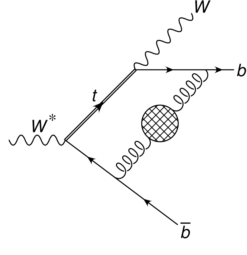
(b)

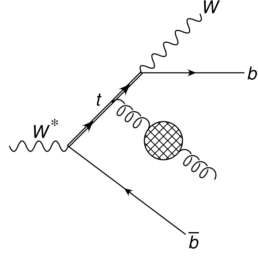
(c)

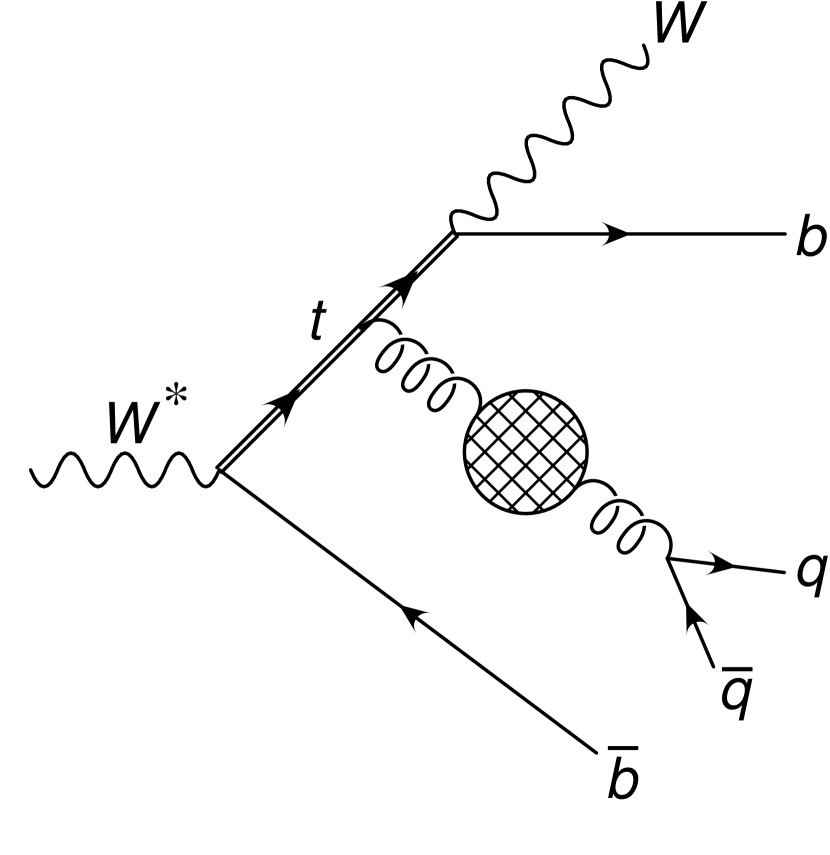
(d)

(e)

Figure 1: Feynman diagram for the Born $W^{*}\to Wb\bar{b}$ process (a), and samples of Feynman diagrams for the virtual contribution (b), for the real-emission contribution (c) and for $W^{*}\to Wb\bar{b}\,q\bar{q}$ production (d).

We want to compute a generic observable, function of the final-state kinematics $\Phi$, that we denote with $O(\Phi)$. We assume the eventual presence of a set of cuts $\Theta(\Phi)$, also function of the final-state kinematics, and define

$$O_{\Theta}(\Phi)=O(\Phi)\times\Theta(\Phi).$$ (8)

The average value of $O$ can be written as

$$\langle O\rangle = N_{\Theta}\left\{\int\mathrm{d}\Phi_{\rm b}\,\sigma_{\rm b}(\Phi_{\rm b})\,O_{\Theta}(\Phi_{\rm b})+\int\mathrm{d}\Phi_{\rm b}\,\sigma_{\rm v}(\Phi_{\rm b})\,O_{\Theta}(\Phi_{\rm b})+\int\mathrm{d}\Phi_{g}\,\sigma_{g}(\Phi_{g})\,O_{\Theta}(\Phi_{g})\right.$$ (9)

$$\hskip 19.91684pt\left.+\int\mathrm{d}\Phi_{q\bar{q}}\,\sigma_{q\bar{q}}(\Phi_{q\bar{q}})\,O_{\Theta}(\Phi_{q\bar{q}})\right\},$$

where the first term represents the Born contribution, the second the virtual one, the third the one due to the emission of a real gluon and the fourth represents the contribution of the real production of $n_{f}$ $q\bar{q}$ pairs. Equation (9) implicitly defines our notation for the different phase space integration volumes.

We always imply that the gluon propagator, in the last three contributions, includes the sum of all vacuum-polarization insertions of light-quark loops.

$N_{\Theta}$ is a normalization factor, given by

$$N_{\Theta}^{-1} = \int\mathrm{d}\Phi_{\rm b}\,\sigma_{\rm b}(\Phi_{\rm b})\,\Theta(\Phi_{\rm b})+\int\mathrm{d}\Phi_{\rm b}\,\sigma_{\rm v}(\Phi_{\rm b})\,\Theta(\Phi_{\rm b})$$ (10)

$$+\int\mathrm{d}\Phi_{g}\,\sigma_{g}(\Phi_{g})\,\Theta(\Phi_{g})+\int\mathrm{d}\Phi_{q\bar{q}}\,\sigma_{q\bar{q}}(\Phi_{q\bar{q}})\,\Theta(\Phi_{q\bar{q}})\,.$$

We can then rewrite eq. (9) as

$$\langle O\rangle = N_{\Theta}\left\{\int\mathrm{d}\Phi_{\rm b}\,\sigma_{\rm b}(\Phi_{\rm b})\,O_{\Theta}(\Phi_{\rm b})+\int\mathrm{d}\Phi_{\rm b}\,\sigma_{\rm v}(\Phi_{\rm b})\,O_{\Theta}(\Phi_{\rm b})\right.+\int\mathrm{d}\Phi_{g}\,\sigma_{g}(\Phi_{g})\,O_{\Theta}(\Phi_{g})$$ (11)

$$+\int\mathrm{d}\Phi_{q\bar{q}}\,\sigma_{q\bar{q}}(\Phi_{q\bar{q}})\,O_{\Theta}\left(\Phi_{g^{*}}\right)+\left.\int\mathrm{d}\Phi_{q\bar{q}}\,\sigma_{q\bar{q}}(\Phi_{q\bar{q}})\,\left[O_{\Theta}(\Phi_{q\bar{q}})-O_{\Theta}(\Phi_{g^{*}})\right]\right\},$$

where we have subtracted and added the same quantity to the $q\bar{q}$ contribution. In the last two lines, $O_{\Theta}(\Phi_{g^{*}})$ is defined in terms of the $\Phi_{g^{*}}$ phase space, that is obtained from the $\Phi_{q\bar{q}}$ phase space by clustering the $q\bar{q}$ pair into a single pseudoparticle, that we denote with $g^{*}$. We also define

$$\langle O\rangle_{\rm v} \equiv N_{\Theta}\int\mathrm{d}\Phi_{\rm b}\,\sigma_{\rm v}(\Phi_{\rm b})\,O_{\Theta}(\Phi_{\rm b})\,,$$ (12)

$$\langle O\rangle_{g} \equiv N_{\Theta}\int\mathrm{d}\Phi_{g}\,\sigma_{g}(\Phi_{g})\,O_{\Theta}(\Phi_{g})+N_{\Theta}\int\mathrm{d}\Phi_{q\bar{q}}\,\sigma_{q\bar{q}}(\Phi_{q\bar{q}})\,O_{\Theta}(\Phi_{g^{*}})\,,$$ (13)

$$\langle O\rangle_{q\bar{q}} \equiv N_{\Theta}\int\mathrm{d}\Phi_{q\bar{q}}\,\sigma_{q\bar{q}}(\Phi_{q\bar{q}})\,\left[O_{\Theta}(\Phi_{q\bar{q}})-O_{\Theta}(\Phi_{g^{*}})\right].$$ (14)

3.1 The normalization factor

The factor $N_{\Theta}$ appearing in eqs. (12)–(14) is in fact simply the inverse of the Born cross section, since the quantities it multiplies are already at NLO level. Thus, in these cases,

$$N_{\Theta}\rightarrow N^{(0)}_{\Theta}=\left\{\int\mathrm{d}\Phi_{\rm b}\,\sigma_{\rm b}(\Phi_{\rm b})\,\Theta\left(\Phi_{\rm b}\right)\right\}^{-1}.$$ (15)

The factor of $N_{\Theta}$ in front of the Born term in eq. (11), on the other hand, generates extra contributions of the form

$$N_{\Theta} = \left\{\int\mathrm{d}\Phi_{\rm b}\,\sigma_{\rm b}\left(\Phi_{\rm b}\right)\Theta\left(\Phi_{\rm b}\right)+\int\mathrm{d}\Phi_{\rm b}\,\sigma_{\rm v}\left(\Phi_{\rm b}\right)\Theta\left(\Phi_{\rm b}\right)+\int\mathrm{d}\Phi_{g}\,\sigma_{g}(\Phi_{g})\Theta\left(\Phi_{g}\right)\right.$$ (16)

$$\left.+\int\mathrm{d}\Phi_{q\bar{q}}\,\sigma_{q\bar{q}}(\Phi_{q\bar{q}})\Theta\left(\Phi_{q\bar{q}}\right)\right\}^{-1}$$

$$= N^{(0)}_{\Theta}\left\{1-N^{(0)}_{\Theta}\left[\int\mathrm{d}\Phi_{\rm b}\,\sigma_{\rm v}\left(\Phi_{\rm b}\right)\Theta\left(\Phi_{\rm b}\right)+\int\mathrm{d}\Phi_{g}\,\sigma_{g}(\Phi_{g})\Theta\left(\Phi_{g}\right)\right.\right.$$

$$\hskip 71.13188pt\left.\left.+\int\mathrm{d}\Phi_{q\bar{q}}\,\sigma_{q\bar{q}}(\Phi_{q\bar{q}})\Theta\left(\Phi_{q\bar{q}}\right)\right]\right\}+\mathcal{O}\left(\alpha_{\mathchoice{\displaystyle}{\scriptstyle}{\scriptscriptstyle}{\scriptscriptstyle}\rm S}^{2}\left(\alpha_{\mathchoice{\displaystyle}{\scriptstyle}{\scriptscriptstyle}{\scriptscriptstyle}\rm S}T_{\mathchoice{\displaystyle}{\scriptstyle}{\scriptscriptstyle}{\scriptscriptstyle}\rm F}\right)^{n}\right),\phantom{aaaa}$$

where

$$T_{\mathchoice{\displaystyle}{\scriptstyle}{\scriptscriptstyle}{\scriptscriptstyle}\rm F}=n_{f}\,T_{\mathchoice{\displaystyle}{\scriptstyle}{\scriptscriptstyle}{\scriptscriptstyle}\rm R}.$$ (17)

This gives rise to a Born term of the form

$${\langle O\rangle_{\rm b}}\equiv N^{(0)}_{\Theta}\int\mathrm{d}\Phi_{\rm b}\,\sigma_{\rm b}(\Phi_{\rm b})\,O_{\Theta}(\Phi_{\rm b})\,,$$ (18)

plus an NLO correction equal to

$$-N^{(0)}_{\Theta}\,{\langle O\rangle_{\rm b}}\left[\int\mathrm{d}\Phi_{\rm b}\,\sigma_{\rm v}(\Phi_{\rm b})\,\Theta(\Phi_{\rm b})+\int\mathrm{d}\Phi_{g}\,\sigma_{g}(\Phi_{g})\,\Theta(\Phi_{g})\,+\int\mathrm{d}\Phi_{q\bar{q}}\,\sigma_{q\bar{q}}(\Phi_{q\bar{q}})\,\Theta(\Phi_{q\bar{q}})\right]\!.$$ (19)

In summary, eq. (11) becomes

$$\langle O\rangle={\langle O\rangle_{\rm b}}\!\!\!\! {}+N^{(0)}_{\Theta}\int\mathrm{d}\Phi_{\rm b}\,\sigma_{\rm v}(\Phi_{\rm b})\left[O_{\Theta}(\Phi_{\rm b})-{\langle O\rangle_{\rm b}}\Theta(\Phi_{\rm b})\right]$$ (20)

$${}+N^{(0)}_{\Theta}\int\mathrm{d}\Phi_{g}\,\sigma_{g}(\Phi_{g})\left[O_{\Theta}(\Phi_{g})-{\langle O\rangle_{\rm b}}\Theta(\Phi_{g})\right]$$

$${}+N^{(0)}_{\Theta}\int\mathrm{d}\Phi_{q\bar{q}}\,\sigma_{q\bar{q}}(\Phi_{q\bar{q}})\left[O_{\Theta}(\Phi_{g^{*}})-{\langle O\rangle_{\rm b}}\Theta(\Phi_{g^{*}})\right]$$

$${}+N^{(0)}_{\Theta}\int\mathrm{d}\Phi_{q\bar{q}}\,\sigma_{q\bar{q}}(\Phi_{q\bar{q}})\,$$

$$\hskip 28.45274pt\times\left\{\left[O_{\Theta}(\Phi_{q\bar{q}})-{\langle O\rangle_{\rm b}}\Theta(\Phi_{q\bar{q}})\right]-\left[O_{\Theta}(\Phi_{g^{*}})-{\langle O\rangle_{\rm b}}\Theta(\Phi_{g^{*}})\right]\right\}\!.\phantom{aaaa}$$

3.2 Final results

In App. B we prove that the full result with the gluon propagator dressed with all fermionic self-energy corrections can be computed in terms of the matrix elements for the process $W^{*}\to Wb\bar{b}$ with the real emission or virtual exchange of one massive gluon of mass $\lambda$, and the matrix element for the $W^{*}\to Wb\bar{b}q\bar{q}$ tree-level process.

The general result for the average value of a generic observable $O$, in the presence of final-state cuts $\Theta$, obtained by combining the results of Sec. 3.1 and App. A and B, is

$$\langle O\rangle={\langle O\rangle_{\rm b}}-\frac{1}{b_{0}\,\alpha_{\mathchoice{\displaystyle}{\scriptstyle}{\scriptscriptstyle}{\scriptscriptstyle}\rm S}}\int_{0}^{\infty}\!\frac{\mathrm{d}\lambda}{\pi}\,\frac{\mathrm{d}\widetilde{T}(\lambda)}{\mathrm{d}\lambda}\,\arctan\frac{\pi\,b_{0}\,\alpha_{\mathchoice{\displaystyle}{\scriptstyle}{\scriptscriptstyle}{\scriptscriptstyle}\rm S}}{1+b_{0}\,\alpha_{\mathchoice{\displaystyle}{\scriptstyle}{\scriptscriptstyle}{\scriptscriptstyle}\rm S}\log\displaystyle{\frac{\lambda^{2}}{\mu_{\mathchoice{\displaystyle}{\scriptstyle}{\scriptscriptstyle}{\scriptscriptstyle}C}^{2}}}},$$ (21)

where

$$\alpha_{\mathchoice{\displaystyle}{\scriptstyle}{\scriptscriptstyle}{\scriptscriptstyle}\rm S}=\alpha_{\mathchoice{\displaystyle}{\scriptstyle}{\scriptscriptstyle}{\scriptscriptstyle}\rm S}(\mu),\quad\quad\mu_{\mathchoice{\displaystyle}{\scriptstyle}{\scriptscriptstyle}{\scriptscriptstyle}C}=\mu\,e^{\frac{C}{2}},\quad\quad C=\frac{5}{3},\quad\quad b_{0}=-\frac{T_{\mathchoice{\displaystyle}{\scriptstyle}{\scriptscriptstyle}{\scriptscriptstyle}\rm F}}{3\pi},$$ (22)

$${\langle O\rangle_{\rm b}} = N^{(0)}_{\Theta}\int\mathrm{d}\Phi_{\rm b}\,\sigma_{\rm b}(\Phi_{\rm b})\,O(\Phi_{\rm b})\,\Theta(\Phi_{\rm b})\,,$$ (23)

$$\widetilde{T}\!\left(\lambda\right) = \widetilde{V}\!\left(\lambda\right)+\widetilde{R}\!\left(\lambda\right)+\widetilde{\Delta}\left(\lambda\right)\,,$$ (24)

$$\widetilde{V}\!\left(\lambda\right) = N^{(0)}_{\Theta}\int\mathrm{d}\Phi_{\rm b}\,\sigma_{\rm v}^{(1)}(\lambda,\Phi_{\rm b})\,\left[O(\Phi_{\rm b})-{\langle O\rangle_{\rm b}}\right]\Theta(\Phi_{\rm b})\,,$$ (25)

$$\widetilde{R}\!\left(\lambda\right) = N^{(0)}_{\Theta}\int\mathrm{d}\Phi_{g^{*}}\,\sigma^{(1)}_{g^{*}}(\lambda,\Phi_{g^{*}})\left[O(\Phi_{g^{*}})-{\langle O\rangle_{\rm b}}\right]\Theta(\Phi_{g^{*}})\,,$$ (26)

$$\widetilde{\Delta}\!\left(\lambda\right) = \,\frac{3\pi}{\alpha_{\mathchoice{\displaystyle}{\scriptstyle}{\scriptscriptstyle}{\scriptscriptstyle}\rm S}T_{\mathchoice{\displaystyle}{\scriptstyle}{\scriptscriptstyle}{\scriptscriptstyle}\rm F}}\,N^{(0)}_{\Theta}\lambda^{2}\int\mathrm{d}\Phi_{q\bar{q}}\,\delta\!\left(\lambda^{2}-k^{2}\right)\sigma^{(2)}_{q\bar{q}}(\Phi_{q\bar{q}})$$ (27)

$$\hskip 28.45274pt\times\left\{\left[O(\Phi_{q\bar{q}})-{\langle O\rangle_{\rm b}}\right]\Theta(\Phi_{q\bar{q}})-\left[O(\Phi_{g^{*}})-{\langle O\rangle_{\rm b}}\right]\Theta(\Phi_{g^{*}})\right\}\,,$$

and $\sigma^{(1)}_{g^{*}}(\lambda,\Phi_{g^{*}})$ and $\sigma_{\rm v}^{(1)}(\lambda,\Phi_{\rm b})$ are the real/virtual corrections to the process $W^{*}\to Wb\bar{b}$ for the emission/exchange of a single gluon with mass $\lambda$, and $\sigma^{(2)}_{q\bar{q}}(\Phi_{q\bar{q}})$ is the tree-level cross section for the process $W^{*}\to Wb\bar{b}q\bar{q}$. We denote with $k$ the four-momentum of the $q\bar{q}$ pair. Notice that, in eq. (21), $\alpha_{\mathchoice{\displaystyle}{\scriptstyle}{\scriptscriptstyle}{\scriptscriptstyle}\rm S}$ in $\widetilde{T}(\lambda)$ cancels against the $1/\alpha_{\mathchoice{\displaystyle}{\scriptstyle}{\scriptscriptstyle}{\scriptscriptstyle}\rm S}$ in front of the integral, and

$$\frac{\alpha_{\mathchoice{\displaystyle}{\scriptstyle}{\scriptscriptstyle}{\scriptscriptstyle}\rm S}}{1+b_{0}\,\alpha_{\mathchoice{\displaystyle}{\scriptstyle}{\scriptscriptstyle}{\scriptscriptstyle}\rm S}\log\displaystyle{\frac{\lambda^{2}}{\mu_{\mathchoice{\displaystyle}{\scriptstyle}{\scriptscriptstyle}{\scriptscriptstyle}C}^{2}}}}=\alpha_{\mathchoice{\displaystyle}{\scriptstyle}{\scriptscriptstyle}{\scriptscriptstyle}\rm S}\!\left(\lambda\,e^{-\frac{C}{2}}\right),$$ (28)

so that the resummed result for $\langle O\rangle$ does not depend upon the value of $\mu$. As discussed in App. B, $\widetilde{T}(\lambda)$ vanishes for large $\lambda$, so that the integral in eq. (21) is convergent.

In order to use the above formulae, we computed analytically the cross sections $\sigma^{(2)}_{q\bar{q}}(\Phi_{q\bar{q}})$, $\sigma^{(1)}_{g^{*}}(\lambda,\Phi_{g^{*}})$ and $\sigma_{\rm v}^{(1)}(\lambda,\Phi_{\rm b})$. Due to the finite gluon mass, only ultraviolet divergences arise in the intermediate steps of the calculation. These divergences were dealt with in dimensional regularization. After the mass renormalization has been carried out (adopting a complex mass Denner:2005fg ; Denner:2006ic in order to account for the finite top width), the UV divergences cancel in the virtual contribution because of the vector nature for the incoming $W^{*}$ current. For reasons that will become clear later, we have also computed the same cross sections for $\lambda=0$. In this case, also soft and collinear divergences are treated in dimensional regularization, and the full result is obtained applying a subtraction method. Notice that, for a finite gluon mass, large logarithms of the mass arise in the real and virtual contributions, that cancel in the sum. In the massless limit, these large cancellations are handled by the subtraction method, and do not affect the accuracy of the result.

We evaluated the scalar integrals using COLLIER Denner:2016kdg . The final numerical implementation has been built using the POWHEG ​BOX ​RES framework Jezo:2015aia .

We performed the phase-space integral for $\widetilde{V}$, $\widetilde{R}$, $\widetilde{\Delta}$ numerically for several values of $\lambda$. For small $\lambda$ both $\widetilde{V}$ and $\widetilde{R}$ have logs of $\lambda$ that cancel in the sum, so that one recovers the result corresponding to the NLO corrections to the $W^{*}\to Wb{\bar{b}}$ process involving the exchange or emission of a single massless gluon. The $\widetilde{\Delta}$ term is instead finite by itself, and vanishes for small $\lambda$. We then combine these results, for each observable, in our function $\widetilde{T}$ that we fit as a function of $\lambda$. This allows us to compute the coefficients of the perturbative expansion of our observable at any order in perturbation theory, and also to determine its asymptotic behaviour.

We find that, in general, the behaviour of $\widetilde{T}$ for small $\lambda$ is given by a constant plus a linear term in $\lambda$. It is this linear term that is associated with linear renormalons. As shown in Sec. 2, these correspond to power suppressed contributions of order $\Lambda^{p}$ with $p=1$, where $\Lambda$ is a typical hadronic scale. Higher values of $p$ arise from higher powers of $\lambda$ in the expansion of $\widetilde{T}$. In the present work, we are interested only in $p=1$, since, because of the size of the top mass, higher values are suppressed by a further $\Lambda/m_{t}$ factor.

The inclusive cross section, with or without cuts, is given by formulae similar to the ones from (23) to (27), setting $O=1$ and omitting the normalization factor $N^{(0)}_{\Theta}$. We then write

$$\sigma=\sigma_{\rm b}-\frac{1}{b_{0}\,\alpha_{\mathchoice{\displaystyle}{\scriptstyle}{\scriptscriptstyle}{\scriptscriptstyle}\rm S}}\int_{0}^{\infty}\!\frac{\mathrm{d}\lambda}{\pi}\,\frac{\mathrm{d}T(\lambda)}{\mathrm{d}\lambda}\arctan\frac{\pi\,b_{0}\,\alpha_{\mathchoice{\displaystyle}{\scriptstyle}{\scriptscriptstyle}{\scriptscriptstyle}\rm S}}{1+b_{0}\,\alpha_{\mathchoice{\displaystyle}{\scriptstyle}{\scriptscriptstyle}{\scriptscriptstyle}\rm S}\log\displaystyle{\frac{\lambda^{2}}{\mu_{\mathchoice{\displaystyle}{\scriptstyle}{\scriptscriptstyle}{\scriptscriptstyle}C}^{2}}}},$$ (29)

where

$$\sigma_{\rm b} = \int\mathrm{d}\Phi_{\rm b}\,\sigma_{\rm b}(\Phi_{\rm b})\,\Theta(\Phi_{\rm b})\,,$$ (30)

$$T(\lambda) = V(\lambda)+{R}\!\left(\lambda\right)+\Delta(\lambda),$$ (31)

$$V(\lambda) = \int\mathrm{d}\Phi_{\rm b}\,\sigma_{\rm v}^{(1)}(\lambda,\Phi_{\rm b})\,\Theta(\Phi_{\rm b})\,,$$ (32)

$$R(\lambda) = \int\mathrm{d}\Phi_{g^{*}}\,\sigma^{(1)}_{g^{*}}(\lambda,\Phi_{g^{*}})\,\Theta(\Phi_{g^{*}})\,,$$ (33)

$$\Delta(\lambda) = \frac{3\pi}{\alpha_{\mathchoice{\displaystyle}{\scriptstyle}{\scriptscriptstyle}{\scriptscriptstyle}\rm S}T_{\mathchoice{\displaystyle}{\scriptstyle}{\scriptscriptstyle}{\scriptscriptstyle}\rm F}}\,\lambda^{2}\int\mathrm{d}\Phi_{q\bar{q}}\;\delta\!\left(\lambda^{2}-k^{2}\right)\sigma_{q\bar{q}}(\Phi_{q\bar{q}})\left[\Theta(\Phi_{q\bar{q}})-\Theta(\Phi_{g^{*}})\right].$$ (34)

We notice that when computing inclusive quantities or quantities that do not depend upon the jet kinematics, the $\widetilde{\Delta}(\lambda)$ and $\Delta(\lambda)$ terms of eqs. (27) and (34) are zero. In these cases, our results can just be expressed as functions of the NLO differential cross section computed with a non-zero gluon mass. In general, however, the $\widetilde{\Delta}(\lambda)$ and $\Delta(\lambda)$ contributions cannot be neglected, since observables built with the full kinematics may differ from those obtained by clustering the $q\bar{q}$ pair into a massive gluon. This was first discussed in Ref. Nason:1995np , in the context of $e^{+}e^{-}$ annihilation into jets.

3.3 Changing the mass scheme

The relation between the pole mass $m$ and the $\overline{\rm MS}$ mass $\overline{m}$ in the large-$n_{f}$ limit is discussed in App. C.2. We have

$$\overline{m}(\mu)=m\left\{1-\alpha_{\mathchoice{\displaystyle}{\scriptstyle}{\scriptscriptstyle}{\scriptscriptstyle}\rm S}\left[r_{f}(m,\mu,\alpha_{\mathchoice{\displaystyle}{\scriptstyle}{\scriptscriptstyle}{\scriptscriptstyle}\rm S})+r_{d}^{\rm(f)}(m,\mu,\alpha_{\mathchoice{\displaystyle}{\scriptstyle}{\scriptscriptstyle}{\scriptscriptstyle}\rm S})\right]+\mathcal{O}(\alpha_{\mathchoice{\displaystyle}{\scriptstyle}{\scriptscriptstyle}{\scriptscriptstyle}\rm S}^{2}(\alpha_{\mathchoice{\displaystyle}{\scriptstyle}{\scriptscriptstyle}{\scriptscriptstyle}\rm S}b_{0})^{n})\right\}\,,$$ (35)

where $r_{f}$ and $r_{d}$ are defined in eqs. (146) and (147) respectively, and $r_{d}^{\rm(f)}$ is the finite part of $r_{d}$, that does not receive any contribution from linear terms in $\lambda$. The $r_{f}$ contribution can be written in the form

$$r_{f}(m,\mu,\alpha_{\mathchoice{\displaystyle}{\scriptstyle}{\scriptscriptstyle}{\scriptscriptstyle}\rm S})=-\frac{1}{b_{0}\,\alpha_{\mathchoice{\displaystyle}{\scriptstyle}{\scriptscriptstyle}{\scriptscriptstyle}\rm S}}\int_{0}^{\infty}\frac{\mathrm{d}\lambda}{\pi}\,\frac{\mathrm{d}\ }{\mathrm{d}\lambda}\left[r_{\lambda,f}\!\left(m,\mu\right)\right]\arctan\frac{\pi\,b_{0}\,\alpha_{\mathchoice{\displaystyle}{\scriptstyle}{\scriptscriptstyle}{\scriptscriptstyle}\rm S}}{1+b_{0}\,\alpha_{\mathchoice{\displaystyle}{\scriptstyle}{\scriptscriptstyle}{\scriptscriptstyle}\rm S}\log\displaystyle{\frac{\lambda^{2}}{\mu_{\mathchoice{\displaystyle}{\scriptstyle}{\scriptscriptstyle}{\scriptscriptstyle}C}^{2}}}},$$ (36)

where (see eq. (150))

$$r_{\lambda,f}\!\left(m,\mu\right)=-\frac{C_{\mathchoice{\displaystyle}{\scriptstyle}{\scriptscriptstyle}{\scriptscriptstyle}\rm F}}{2}\frac{\lambda}{m}+{\cal O}\left(\lambda^{2}\right)\,.$$ (37)

Note that the $\mu$ dependence disappears in the leading term. The ${\cal O}(\lambda)$ term in eq. (37) is responsible for the presence of a linear renormalon in the relation between the pole mass and the $\overline{\rm MS}$ one.

In the present work we deal with the finite width of the top quark by using the complex mass scheme Denner:2005fg ; Denner:2006ic . Thus, in our mass relation, both $m$ and $\overline{m}$ are complex, and also $r_{f}$ and $r_{d}$.

Given a result for a quantity $\langle O\rangle$ expressed in terms of the pole mass, representing the average value of some kinematic quantity (possibly including cuts and possibly normalized to the total cross section), in order to find its expression in terms of the $\overline{\rm MS}$ mass we need to Taylor-expand its mass dependence in its leading order expression, and multiply it by the appropriate mass correction. In order to do so, we express $O$ in terms of the pole mass and its complex conjugate, as if they were independent variables (one can think of $m$ appearing in the amplitude, and $m^{*}$ appearing in its complex conjugate). Denoting with ${\langle O\rangle_{\rm b}}$ the LO prediction, we can write

$${\langle O\rangle_{\rm b}}(m,m^{*})\! = \!{\langle O\rangle_{\rm b}}(\overline{m},\overline{m}^{*})+\left\{\frac{\partial{\langle O\rangle_{\rm b}}(\overline{m},\overline{m}^{*})}{\partial\overline{m}}\left(m-\overline{m}\right)+{\rm cc}\right\}$$

$$\approx \!{\langle O\rangle_{\rm b}}(\overline{m},\overline{m}^{*})+\left\{\frac{\partial{\langle O\rangle_{\rm b}}(m,m^{*})}{\partial m}\left(m-\overline{m}\right)+{\rm cc}\right\}$$

$$= \!{\langle O\rangle_{\rm b}}(\overline{m},\overline{m}^{*})+\alpha_{\mathchoice{\displaystyle}{\scriptstyle}{\scriptscriptstyle}{\scriptscriptstyle}\rm S}\!\left\{\frac{\partial{\langle O\rangle_{\rm b}}(m,m^{*})}{\partial m}\,m\!\left[r_{f}(m,\mu,\alpha_{\mathchoice{\displaystyle}{\scriptstyle}{\scriptscriptstyle}{\scriptscriptstyle}\rm S})+r^{\rm(f)}_{d}(m,\mu,\alpha_{\mathchoice{\displaystyle}{\scriptstyle}{\scriptscriptstyle}{\scriptscriptstyle}\rm S})\right]\!+{\rm cc}\right\}\!,$$

where we have neglected $\alpha_{\mathchoice{\displaystyle}{\scriptstyle}{\scriptscriptstyle}{\scriptscriptstyle}\rm S}^{2}(\alpha_{\mathchoice{\displaystyle}{\scriptstyle}{\scriptscriptstyle}{\scriptscriptstyle}\rm S}b_{0})^{n}$ terms and we have dropped the $\mu$ dependence in $\overline{m}$ for ease of notation. Notice that, as far as the linear term in $\lambda$ is concerned, we get the simplified form

$${\langle O\rangle_{\rm b}}(m,m^{*})\! = \!{\langle O\rangle_{\rm b}}(\overline{m},\overline{m}^{*})+\left[\frac{\partial{\langle O\rangle_{\rm b}}(m,m^{*})}{\partial m}+{\rm cc}\right]$$ (39)

$$\times \!\!\left(-\frac{1}{b_{0}\,\alpha_{\mathchoice{\displaystyle}{\scriptstyle}{\scriptscriptstyle}{\scriptscriptstyle}\rm S}}\right)\!\int_{0}^{\infty}\!\frac{\mathrm{d}\lambda}{\pi}\,\frac{\mathrm{d}\ }{\mathrm{d}\lambda}\!\left[-\alpha_{\mathchoice{\displaystyle}{\scriptstyle}{\scriptscriptstyle}{\scriptscriptstyle}\rm S}\frac{C_{\mathchoice{\displaystyle}{\scriptstyle}{\scriptscriptstyle}{\scriptscriptstyle}\rm F}}{2}\lambda\right]\arctan\frac{\pi\,b_{0}\,\alpha_{\mathchoice{\displaystyle}{\scriptstyle}{\scriptscriptstyle}{\scriptscriptstyle}\rm S}}{1+b_{0}\,\alpha_{\mathchoice{\displaystyle}{\scriptstyle}{\scriptscriptstyle}{\scriptscriptstyle}\rm S}\log\displaystyle{\frac{\lambda^{2}}{\mu_{\mathchoice{\displaystyle}{\scriptstyle}{\scriptscriptstyle}{\scriptscriptstyle}C}^{2}}}}\,.$$

Furthermore, we have

$$\frac{\partial{\langle O\rangle_{\rm b}}(m,m^{*})}{\partial m}+{\rm cc}=\frac{\partial{\langle O\rangle_{\rm b}}(m,m^{*})}{\partial\,{\rm Re}(m)}.$$ (40)

Thus, when going from the pole to the $\overline{\rm MS}$ mass scheme, the definition for $\widetilde{T}$ is modified for small $\lambda$ into

$$\widetilde{T}(\lambda)\to\widetilde{T}(\lambda)-\frac{\partial{\langle O\rangle_{\rm b}}(m,m^{*})}{\partial\,{\rm Re}(m)}\,\frac{C_{\mathchoice{\displaystyle}{\scriptstyle}{\scriptscriptstyle}{\scriptscriptstyle}\rm F}\alpha_{\mathchoice{\displaystyle}{\scriptstyle}{\scriptscriptstyle}{\scriptscriptstyle}\rm S}}{2}\,\lambda+{\cal O}\!\left(\lambda^{2}\right)\,.$$ (41)

One may wonder where the ${\langle O\rangle_{\rm b}}$ subtraction term, that is present by definition in $\widetilde{T}$, is hiding here. In fact, in the case of normalized observables, it should be kept in mind that ${\langle O\rangle_{\rm b}}$ includes a division by the total cross section. When taking the derivative, the denominator is also derived, yielding the ${\langle O\rangle_{\rm b}}$ subtraction term.

This procedure is still valid for a generic observable $O$ that does not involve the normalization factor $N_{\Theta}$, like the total cross section, so also in this case we need to replace $T$ with

$$T(\lambda)\to T(\lambda)-\frac{\partial O_{\rm b}(m,m^{*})}{\partial\,{\rm Re}(m)}\,\frac{C_{\mathchoice{\displaystyle}{\scriptstyle}{\scriptscriptstyle}{\scriptscriptstyle}\rm F}\alpha_{\mathchoice{\displaystyle}{\scriptstyle}{\scriptscriptstyle}{\scriptscriptstyle}\rm S}}{2}\,\lambda+{\cal O}\!\left(\lambda^{2}\right)\,.$$ (42)

Notice that the same expression holds for $\widetilde{T}$ and $T$.

We also stress that eqs. (41) and (42) also apply to any so called “short distance” mass schemes Czarnecki:1997sz ; Beneke:1998rk ; Hoang:1998ng ; Pineda:2001zq ; Fleming:2007qr ; Jain:2008gb ; Hoang:2008yj . These schemes are such that no mass renormalon affects their definition, and of course in order for this to be the case, their small $\lambda$ behaviour should be the same one of the $\overline{\rm MS}$ scheme.

4 Physical objects

The numerical values of the parameters used in our study are given by

$$m_{\mathchoice{\displaystyle}{\scriptstyle}{\scriptscriptstyle}{\scriptscriptstyle}0} = 172.5\,{\rm GeV},$$ (43)

$$\Gamma_{t} = 1.3279\,{\rm GeV},$$ (44)

$$m = \sqrt{m_{\mathchoice{\displaystyle}{\scriptstyle}{\scriptscriptstyle}{\scriptscriptstyle}0}^{2}-im_{\mathchoice{\displaystyle}{\scriptstyle}{\scriptscriptstyle}{\scriptscriptstyle}0}\Gamma_{t}},$$ (45)

$$m_{\mathchoice{\displaystyle}{\scriptstyle}{\scriptscriptstyle}{\scriptscriptstyle}W} = 80.419\,{\rm GeV},$$ (46)

$$E_{\mathchoice{\displaystyle}{\scriptstyle}{\scriptscriptstyle}{\scriptscriptstyle}\rm CM} = 300\,{\rm GeV},$$ (47)

$$\mu = m_{\mathchoice{\displaystyle}{\scriptstyle}{\scriptscriptstyle}{\scriptscriptstyle}0}\,.$$ (48)

Furthermore we have set $n_{l}=5$ and, from $\alpha_{\mathchoice{\displaystyle}{\scriptstyle}{\scriptscriptstyle}{\scriptscriptstyle}\rm S}(M_{\mathchoice{\displaystyle}{\scriptstyle}{\scriptscriptstyle}{\scriptscriptstyle}Z})=0.1181$, we have

$$\alpha_{\mathchoice{\displaystyle}{\scriptstyle}{\scriptscriptstyle}{\scriptscriptstyle}\rm S}(\mu)=0.108\,.$$ (49)

4.1 Selection cuts

In order to better mimic realistic experimental analyses adopted at hadron colliders, at times we introduce selection cuts for our cross sections, requiring the presence of a $b$ jet and a (separated) $\bar{b}$ jet, both having energy greater than 30 GeV. Jets are reconstructed using the Fastjet Cacciari:2011ma implementation of the anti-$k_{t}$ algorithm Cacciari:2008gp for $e^{+}e^{-}$ collisions, for various values of the radius parameter $R$.

5 Inclusive cross section

The formula for the inclusive cross section is given in eq. (29), that will be applied both without and with cuts.

5.1 Inclusive cross section without cuts

In the absence of cuts, the expression for $T(\lambda)$ in eq. (31) simplifies, since $\Delta(\lambda)$, given by eq. (34), is identically zero. Its small $\lambda$ behaviour is shown in Fig. 2.

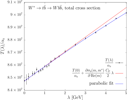
Figure 2: Small $\lambda$ behaviour of $T(\lambda)$ for the total cross section as function of the gluon mass $\lambda$. In black the data points computed with our numerical calculations, in red the linear $\lambda$ dependence and in blue the parabolic fit of the points. The $\lambda=0$ point has been obtained by performing the standard NLO computation in dimensional regularization.

From the figure we can see that the error on $T(\lambda)$ increases for small $\lambda$. However, the point at $\lambda=0$ is directly computed with a massless gluon, by dealing with the soft and collinear singularities with the usual dimensional regularization techniques, and has negligible error. As discussed in Sec. 3.3, the same calculation performed in the $\overline{\rm MS}$ mass scheme would yield, for the total cross section, to the replacement given in eq. (42)

$$T(\lambda)\to T(\lambda)-\frac{\partial\sigma_{b}(m,m^{*})}{\partial\,{\rm Re}(m)}\,\frac{C_{\mathchoice{\displaystyle}{\scriptstyle}{\scriptscriptstyle}{\scriptscriptstyle}\rm F}\alpha_{\mathchoice{\displaystyle}{\scriptstyle}{\scriptscriptstyle}{\scriptscriptstyle}\rm S}}{2}\,\lambda+{\cal O}\!\left(\lambda^{2}\right).$$ (50)

So, in the same figure, we also plot (in red) the expression

$$T(0)+\frac{\partial\sigma_{b}(m,m^{*})}{\partial\,{\rm Re}(m)}\,\frac{C_{\mathchoice{\displaystyle}{\scriptstyle}{\scriptscriptstyle}{\scriptscriptstyle}\rm F}\alpha_{\mathchoice{\displaystyle}{\scriptstyle}{\scriptscriptstyle}{\scriptscriptstyle}\rm S}}{2}\,\lambda\,.$$ (51)

Since this coincides with $T(\lambda)$ for small $\lambda$, we infer that the $\overline{\rm MS}$ result has no linear term in $\lambda$, so that no linear renormalons arise for the total cross section in the $\overline{\rm MS}$ scheme. From the figure it is also clear that this holds for both $\lambda\lesssim\Gamma_{t}$ and for $\lambda\gg\Gamma_{t}$, where $\Gamma_{t}$ is the top width. The $\lambda\lesssim\Gamma_{t}$ behaviour is justified by the fact that, because of the finite width, phase-space points where the top is on shell are never reached (see App. D). Thus, no linear renormalon is present unless one uses the pole-mass scheme, that has a linear renormalon in the counterterm.

As far as the $\lambda\gg\Gamma_{t}$ limit is concerned, we notice that the $\lambda$ behaviour should be the same as that of the narrow width approximation (NWA), where the cross section factorizes in terms of the on-shell top-production cross section, and its decay partial width

$$\sigma\!\left(W^{*}\rightarrow Wb\bar{b}\right)=\sigma\!\left(W^{*}\rightarrow t\bar{b}\right)\frac{\Gamma(t\rightarrow Wb)}{\Gamma_{t}}+\mathcal{O}\left(\frac{\Gamma_{t}}{m}\right).$$ (52)

The behaviour of $T(\lambda)$, computed either exactly or in the NWA, is shown in Fig. 3.

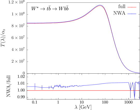
Figure 3: $T(\lambda)$ for the NLO total cross section, as function of the gluon mass $\lambda$, computed in the pole-mass scheme using the exact full matrix elements, in red, and the narrow-width approximation, NWA, in blue.

The factor $\sigma(W^{*}\rightarrow t\bar{b})$ is clearly free of linear renormalons, since it is a totally inclusive decay of a colour-neutral system. Although less obvious, this is also the case for the factor $\Gamma(t\rightarrow Wb)$ (see Refs. Bigi:1994em ; Beneke:1994bc ; Beneke:1994qe ).

5.2 Inclusive cross section with cuts

When the selection cuts discussed in Sec. 4.1 are imposed, the cross section depends explicitly upon the jet radius $R$. We expect that jets requirements will induce the presence of linear renormalons, and thus linear small-$\lambda$ behaviour of $T$, with a slope that goes like $1/R$ for small $R$ Dasgupta:2007wa .

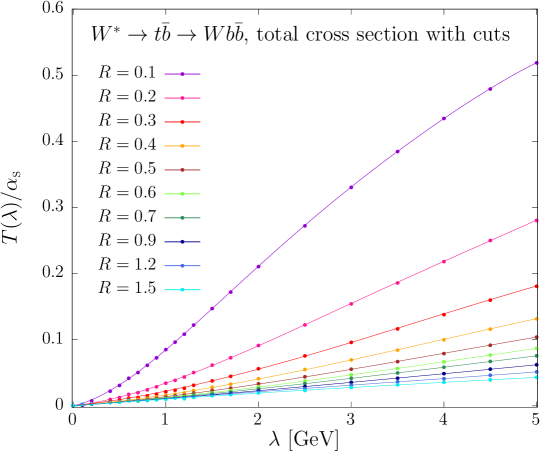
Figure 4: Small $\lambda$ behaviour for $T(\lambda)$ for the inclusive cross section with cuts, for several jet radii. The points are obtained with our numerical calculations, while the solid lines represent their polynomial fit. The fitting functions are order 5, 4 and 3 polynomials for $R=0.1$, $R=0.2$ and $R\geq 0.3$ radii respectively.

In Fig. 4 we display the small $\lambda$ behaviour for $T(\lambda)$ for the inclusive cross section with cuts, for several jet radii. Together with the results of our calculation, we also plot, for each value of $R$, a polynomial fit to the data.

When changing from the pole to the $\overline{\rm MS}$-mass scheme, we only expect a mild $R$ dependent correction to the slope of $T(\lambda)$ at $\lambda=0$, and thus we cannot expect the same benefit that we observed for the cross section without cuts.

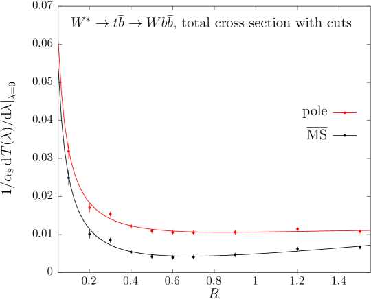
Figure 5: $R$ dependence of the slope of $T(\lambda)$ for the inclusive cross section, at $\lambda=0$, using the pole (red) or the $\overline{\rm MS}$ mass scheme (black). The solid lines represent fits of parametric form $a/R+b+c\,R+d\,R^{2}$.

This is illustrated in Fig. 5 for several jet radii. The $1/R$ behaviour is clearly visible. In addition, for relatively large-$R$ values, the use of the $\overline{\rm MS}$ scheme brings about some reduction to the slope of the linear term. This may be due to the fact that the cross section with cuts captures a good part of the cross section without cuts, and thus it partially inherits its benefits when changing scheme. However, it is also clear that linear non-perturbative ambiguities remain important also in the $\overline{\rm MS}$ scheme when cuts are involved.

6 Reconstructed-top mass

In this section we consider the average value $\langle M\rangle$, where $M$ is the mass of the system comprising the $W$ boson and the $b$ jet. Such observable is closely related to the top mass, and, on the other hand, is simple enough to be easily computed in our framework. We use the same selection cuts described previously.

We computed $\langle M\rangle$ also in the narrow width limit, by simply setting the top width to $10^{-3}$ GeV. In this limit, top production and decay factorize, so that we have an unambiguous assignment of the final state partons to the top decay products. We first compute $\langle M\rangle$ in the narrow width limit, using only the top decay products, and without applying any cuts. We then compute it again, still using only the top decay products, but introducing our standard cuts. Finally we compute it again using all decay products and our standard cuts.

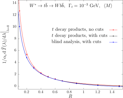
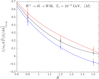
Figure 6: $R$ dependence of the slope of $\widetilde{T}(\lambda)$ for the average reconstructed mass $\langle M\rangle$, at $\lambda=0$, computed with $\Gamma_{t}=10^{-3}$ GeV. The results obtained by reconstructing the $b$ jet using only the top-decay products, without imposing any cut and with the cuts of Sec. 4.1, are shown in red and in black, respectively. In blue, the results for a blind analysis with cuts. The solid lines represent fits of parametric form $a/R+b+c\,R+d\,R^{2}$. The black and the blue curves are almost completely overlapping and are indistinguishable in the plot on the left. A blowup of the high-$R$ region is illustrated in the plot on the right.

The results of these calculations are reported in Fig. 6, where the slope at $\lambda=0$ of $\widetilde{T}$ for our observable is plotted as a function of the jet radius $R$. As expected we see the shape proportional to $1/R$ for small $R$ Dasgupta:2007wa .

In the case of the calculation of $\langle M\rangle$ performed using only the top decay products, and without any cuts, we expect that, for large values of $R$, the average value of $M$ should get closer and closer to the input top pole mass, irrespective of the value of $\lambda$. Thus, the slope of $\widetilde{T}(\lambda)$ for $\lambda=0$ should become smaller and smaller. We find in this case that, for the largest value of $R$ we are using ($R=1.5$), the slope has a value around 0.09. When cuts are introduced this value becomes even smaller, around 0.04. This curve is fairly close to the one obtained using all final-state particles and including cuts. The large-$R$ value in this case is $-0.08$.

If we change scheme from the pole mass to the $\overline{\rm MS}$ one, the corresponding change of $\widetilde{T}$ is given by eq. (41), and, for the observable at hand, the derivative term is very near 1. The change in slope when going to the $\overline{\rm MS}$ scheme is roughly $-C_{\mathchoice{\displaystyle}{\scriptstyle}{\scriptscriptstyle}{\scriptscriptstyle}\rm F}/2\approx-0.67$. Thus, if we insisted in using the $\overline{\rm MS}$ mass for the present observable, for large jet radii, we would get an ambiguity larger than if we used the pole mass scheme. The same holds even if we employ a finite top width, as shown in Fig. 7, where the $R$ dependence of the $\widetilde{T}(\lambda)$ slope for $\Gamma_{t}=1.3279$ GeV is plotted.

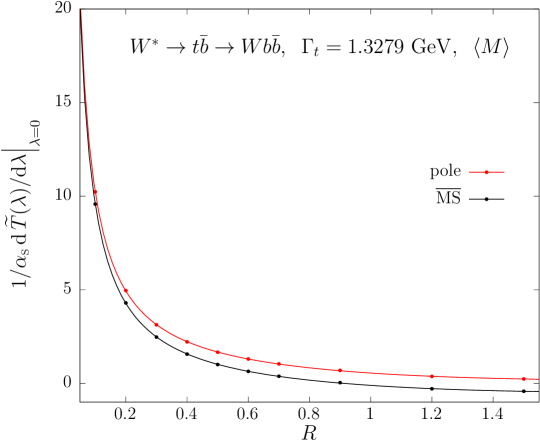
Figure 7: $R$ dependence of the slope of $\widetilde{T}$ for the averaged reconstructed mass $M$. The solid lines are the result of a fit of the form $a/R+b+c\,R+d\,R^{2}$.

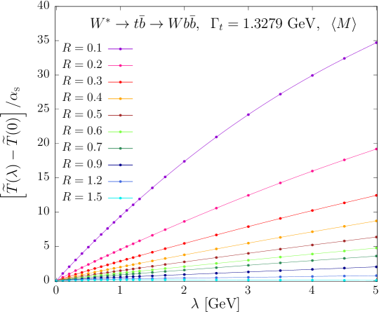
Figure 8: Small $\lambda$ behaviour of $\widetilde{T}(\lambda)$ for the averaged reconstructed-top mass, for several values of the jet radius $R$. The solid lines represent the polynomial fit of the computed points. For $R\geq 1.2$ a $4^{\rm th}$ order polynomial is adopted, while for the other $R$ values a $5^{\rm th}$ order polynomial is employed.

In Fig. 8 we plot the small $\lambda$ behaviour of $\widetilde{T}(\lambda)$ for the reconstructed-top mass, computed with the finite top width, for several values of the jet radius $R$. It is clear that our observable is strongly affected by the jet renormalon. The same plot for only the three largest values of $R$ is shown in Fig. 9.

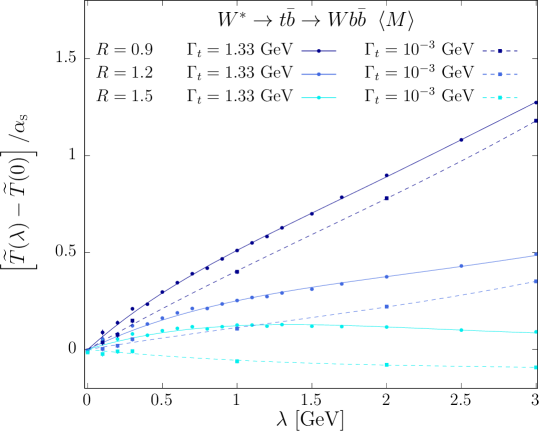
Figure 9: Small $\lambda$ behaviour of $\widetilde{T}(\lambda)$ for the averaged reconstructed-top mass for large values of the jet radius $R$, for two different values of the top decay width, $\Gamma_{t}=1.3279$ GeV (solid lines) and $\Gamma_{t}=10^{-3}$ GeV (dashed lines). The dashed lines are a cubic fit of the computed points. The solid lines are the same displayed in Fig. 8.

The figure shows clearly that the slope of $\widetilde{T}(\lambda)$ for small $\lambda$ computed with $\Gamma_{t}=1.3279$ GeV changes when $\lambda$ goes below $1$ GeV, that is to say, when it goes below the top width. This behaviour is expected, since the top width acts as a cutoff on soft radiation. In the figure we also report the $\lambda$ behaviour in the narrow-width approximation. It is evident that the slopes computed in this limit are similar to the slopes with $\Gamma_{t}=1.3279$ GeV, for values of $\lambda$ larger than the top width. It is also clear that the slopes that we find here for the largest $R$ value are considerably smaller than the slope change induced by a change to a short distance mass scheme, that amounts to $-0.67$. In other words, the pole mass scheme is more appropriate for this observable, irrespective of finite width effects.

We notice that, in the present case, for values of $R$ below 1, the $\overline{\rm MS}$ scheme seems to be better, because of a cancellation of the $R$ dependent renormalon and the mass one. From our study, however, it clearly emerges that such cancellation is accidental, and one should not rely upon it to claim an increase in accuracy.

7 $\boldsymbol{W}$ boson energy

In this section we study the behaviour of the average value of the $W$ energy, $E_{\mathchoice{\displaystyle}{\scriptstyle}{\scriptscriptstyle}{\scriptscriptstyle}W}$. This observable does not depend upon the jet definition, and can thus be considered a representative of pure “leptonic” observables in top-mass measurements. In this study, we do not apply any cut, in order to avoid jet renormalons. Our goal is to see if this observable is free of renormalons in some mass scheme.

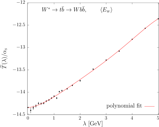
Figure 10: Small $\lambda$ behaviour of $\widetilde{T}(\lambda)$ for $\langle E_{\mathchoice{\displaystyle}{\scriptstyle}{\scriptscriptstyle}{\scriptscriptstyle}W}\rangle$. The solid line represents a $5^{\rm th}$ order polynomial fit.

In order to change scheme, according to eq. (41), we need the derivative of the Born value of the observable with respect to the real part of the top mass. We have computed numerically this quantity, and found the value

$$\frac{\partial\langle E_{\mathchoice{\displaystyle}{\scriptstyle}{\scriptscriptstyle}{\scriptscriptstyle}W}\rangle_{b}}{\partial\,{\rm Re}(m)}=0.0980\,(8)\,.$$ (53)

The small-$\lambda$ dependence of the corresponding $\widetilde{T}$ function is shown in Fig. 10. For values of $\lambda$ much larger than the width, the slope of the curve is roughly 0.45. Thus, under these conditions, a renormalon is clearly present whether we use the pole or the $\overline{\rm MS}$ scheme, since the correction in slope due to the use of the latter would be $-0.098\times C_{\mathchoice{\displaystyle}{\scriptstyle}{\scriptscriptstyle}{\scriptscriptstyle}\rm F}/2=-0.065$.

For $\lambda$ below the top width we see a reduction in slope, that is too difficult to estimate because of the lack of statistics. In order to check that the change in slope is related to the top finite width, we ran the program with a reduced $\Gamma_{t}$, expecting to see a constant slope extending down to smaller values of $\lambda$. This is illustrated in Fig. 11.

Figure 11: Small $\lambda$ behaviour of $\widetilde{T}(\lambda)$ for $\langle E_{\mathchoice{\displaystyle}{\scriptstyle}{\scriptscriptstyle}{\scriptscriptstyle}W}\rangle$, for increasingly smaller values of $\Gamma_{t}$. The blue and the black solid lines are a parabolic fit of the computed points, the red line is the same one displayed in Fig. 10.

We clearly see that, as $\Gamma_{t}$ becomes smaller, the slope of the $\lambda$ dependence remains constant, near the value $0.45$ found before, down to smaller values of $\lambda$. Since we have that

$$\frac{\partial\langle E_{\mathchoice{\displaystyle}{\scriptstyle}{\scriptscriptstyle}{\scriptscriptstyle}W}\rangle_{b}}{\partial\,{\rm Re}(m)} = 0.098\,(4)\,,\quad{\rm for}\quad\Gamma_{t}=0.1\leavevmode\nobreak\ {\rm GeV},$$ (54)

$$\frac{\partial\langle E_{\mathchoice{\displaystyle}{\scriptstyle}{\scriptscriptstyle}{\scriptscriptstyle}W}\rangle_{b}}{\partial\,{\rm Re}(m)} = 0.10\,(3)\,,\phantom{0}\quad{\rm for}\quad\Gamma_{t}=0.01\leavevmode\nobreak\ {\rm GeV},$$ (55)

it is clear that, for a vanishing top width, $\langle E_{W}\rangle$ has linear renormalons both in the $\overline{\rm MS}$ and pole mass scheme.

We also performed a run with $\Gamma_{t}=10$ GeV and $\Gamma_{t}=20$ GeV, in order to estimate more accurately the value of the slope for $\lambda\ll\Gamma_{t}$.

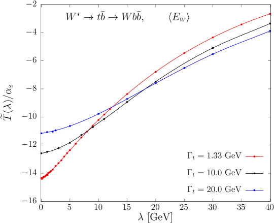
Figure 12: Results for the small $\lambda$ behaviour of $\widetilde{T}$ for $\langle E_{\mathchoice{\displaystyle}{\scriptstyle}{\scriptscriptstyle}{\scriptscriptstyle}W}\rangle$, at different values of $\Gamma_{t}$. The error bar associated to each point computed at a given value of $\lambda$ is also plotted, but is too small to be visible on the scale of the figure. The red line ($\Gamma_{t}=1.33$ GeV) is a $5^{\rm th}$ order polynomial fit for $\lambda\leq 5$ GeV and a spline for larger $\lambda$ values. The blue and the black solid lines, that interpolates the results obtained with $\Gamma_{t}=10$ GeV and $\Gamma_{t}=20$ GeV respectively, are a cubic fit for $\lambda<\Gamma_{t}$ and a spline for $\lambda>\Gamma_{t}$.

The results are shown in Fig. 12. In Tab. 1 we illustrate the slopes of $\widetilde{T}(\lambda)$ for small $\lambda$, obtained from the polynomial interpolation displayed in Fig. 12, and the corresponding value in the $\overline{\rm MS}$ scheme, obtained by adding $-\frac{C_{\mathchoice{\displaystyle}{\scriptstyle}{\scriptscriptstyle}{\scriptscriptstyle}\rm F}}{2}\frac{\partial\langle E_{\mathchoice{\displaystyle}{\scriptstyle}{\scriptscriptstyle}{\scriptscriptstyle}W}\rangle_{b}}{\partial\,{\rm Re}(m)}$ to the fitted slope. This shows that the linear sensitivity largely cancels in the $\overline{\rm MS}$ scheme.

$\Gamma_{t}$	slope (pole)	$\displaystyle\frac{\partial\langle E_{\mathchoice{\displaystyle}{\scriptstyle}{\scriptscriptstyle}{\scriptscriptstyle}W}^{\phantom{\big{(}}}\rangle_{b}}{\partial\,{\rm Re}(m)}$	$\displaystyle-\frac{C_{\mathchoice{\displaystyle}{\scriptstyle}{\scriptscriptstyle}{\scriptscriptstyle}\rm F}}{2}\frac{\partial\langle E_{\mathchoice{\displaystyle}{\scriptstyle}{\scriptscriptstyle}{\scriptscriptstyle}W}\rangle_{b}}{\partial\,{\rm Re}(m)}_{\phantom{\big{(}}}$	slope ($\overline{\rm MS}$)
10 GeV	$0.058\,(8)$	$0.0936\,(4)$	$-0.0624\,(3)$	$0.004\,(8)$
20 GeV	$0.061\,(2)$	$0.0901\,(2)$	$-0.0601\,(1)$	$0.001\,(2)$

Table 1: Slopes for $\widetilde{T}(\lambda)$ computed for $\langle E_{\mathchoice{\displaystyle}{\scriptstyle}{\scriptscriptstyle}{\scriptscriptstyle}W}\rangle$ in the pole-mass scheme and the derivative terms needed to change to the $\overline{\rm MS}$ one, for large top widths.

One may now wonder if this cancellation is exact, or just accidental. In fact, we prove in App. D that the cancellation is exact.

8 All-orders expansion in $\boldsymbol{\alpha_{\mathchoice{\displaystyle}{\scriptstyle}{\scriptscriptstyle}{\scriptscriptstyle}\rm S}}$

We consider now the all-orders expansion of various quantities, in order to see how it is affected by the infrared renormalons, both in the pole and in the $\overline{\rm MS}$-mass scheme.

One may think that in our framework we could, for example, compute a mass sensitive observable, extract the mass (for a given value of the observable) in different schemes, and finally convert all results to the pole mass scheme, thus assessing the reliability of the methods used to estimate the renormalon ambiguity in the pole mass Pineda:2001zq ; Ayala:2014yxa ; Beneke:2016cbu ; Hoang:2017btd . In fact, within the large-$n_{f}$ approximation, if the method adopted to resum the perturbative expansion is linear, as is the case of the Borel transform method, we should find identical results (always in the large-$n_{f}$ sense) in the $\overline{\rm MS}$ and the pole-mass schemes. In fact, following eq. (3.3), the relation between the pole and $\overline{\rm MS}$-mass scheme, for a generic observable, is given by

$${\langle O\rangle_{\rm b}}(m,m^{*})+\alpha_{\mathchoice{\displaystyle}{\scriptstyle}{\scriptscriptstyle}{\scriptscriptstyle}\rm S}\,\langle\,O\rangle^{(1)}(m,m^{*}) = {\langle O\rangle_{\rm b}}(\overline{m},\overline{m}^{*})+\left[\frac{\partial{\langle O\rangle_{\rm b}}(m,m^{*})}{\partial m}(m-\overline{m})+{\rm cc}\right]$$ (56)

$${}+\alpha_{\mathchoice{\displaystyle}{\scriptstyle}{\scriptscriptstyle}{\scriptscriptstyle}\rm S}\,\langle O\rangle^{(1)}(m,m^{*})+{\cal O}\left(\alpha_{\mathchoice{\displaystyle}{\scriptstyle}{\scriptscriptstyle}{\scriptscriptstyle}\rm S}^{2}\left(b_{0}\alpha_{\mathchoice{\displaystyle}{\scriptstyle}{\scriptscriptstyle}{\scriptscriptstyle}\rm S}\right)^{n}\right).$$

Neglecting subleading terms, this is an identity, since the expansion of ${\langle O\rangle_{\rm b}}$ in the mass difference stops at the first order in the large-$n_{f}$ limit. When performing the calculation in the pole-mass scheme, we need to resum the expansion of $\langle O\rangle^{(1)}$, while if we perform the calculation in the $\overline{\rm MS}$ scheme, we are resumming the expansion of the sum of terms in the curly bracket. If the resummation method is linear, this last resummation can be performed on the individual terms inside the curly bracket. This is exactly what we would do on the left-hand side if, after the resummation, we wanted to express the same result in the $\overline{\rm MS}$ scheme. In other words, if one uses the Borel method to perform the resummation, and defines the pole mass to be the sum of the mass relation formula eq. (35), all results obtained in the $\overline{\rm MS}$ scheme would be identical to those obtained in the pole mass scheme up to terms of relative order $\alpha_{\mathchoice{\displaystyle}{\scriptstyle}{\scriptscriptstyle}{\scriptscriptstyle}\rm S}C_{\mathchoice{\displaystyle}{\scriptstyle}{\scriptscriptstyle}{\scriptscriptstyle}\rm F}$, provided the same Borel sum method is used also for the observables.

In the following we will estimate the terms of the perturbative expansion by extrapolating our large-$n_{f}$ results to the realistic QCD case, (i.e. in the large-$b_{0}$ approximation). In order to do this, we will replace the $b_{0}$ of the large-$n_{f}$ theory with the $b_{0}$ of QCD, and perform other minor adjustments, detailed later. Needless to say, corrections to the large-$b_{0}$ approximation may be non-negligible. We thus expect that, by changing scheme, we will generate potentially important differences. These differences should not therefore be interpreted as due to large ambiguities related to the choice of mass scheme, but rather to the violation of the large-$b_{0}$ approximation.

The procedure we adopt in order to compute the terms of the perturbative expansion follows from eq. (21). We fit numerically the $\lambda$ dependence of the appropriate $T$ or $\widetilde{T}$ function, and we take the derivative of the fit. The arctangent factor is instead expanded analytically, and the integration is performed numerically for each perturbative order. The details of the procedure that we followed in order to go from the large-$n_{f}$ theory to the large-$b_{0}$ approximation are described at the end of App. A, eqs. (70) to (74).

8.1 Mass-conversion formula

The procedure for the calculation of the mass-conversion formula is described in App. C.2. Here we switch to the realistic $b_{0}$ and $C$ values as discussed in the previous section. The expansion of the mass conversion formula reads

$$\overline{m}(\mu)=m\left(1-\sum_{i=1}^{\infty}c_{i}\,\alpha_{\mathchoice{\displaystyle}{\scriptstyle}{\scriptscriptstyle}{\scriptscriptstyle}\rm S}^{i}\right).$$ (57)

and the $c_{i}$ coefficients are tabulated in Tab. 2, with $\mu^{2}={\rm Re}(m^{2})=m_{0}^{2}$, where $m_{0}$ is given in eq. (43).

$\displaystyle\phantom{\Big{|}}m-\overline{m}(\mu)\phantom{\Big{|}}$
$\phantom{\Big{|}}i\phantom{\Big{|}}$	${\rm Re}\left(c_{i}\right)$	${\rm Im}\left(c_{i}\right)$	${\rm Re}\left(m\,c_{i}\,\alpha_{\mathchoice{\displaystyle}{\scriptstyle}{\scriptscriptstyle}{\scriptscriptstyle}\rm S}^{i}\right)$	${\rm Im}\left(m\,c_{i}\,\alpha_{\mathchoice{\displaystyle}{\scriptstyle}{\scriptscriptstyle}{\scriptscriptstyle}\rm S}^{i}\right)$
— 1 —	$4.244\times 10^{-1}$	$2.450\times 10^{-3}$	$7.919\times 10^{+0}$	$+1.524\times 10^{-2}$
— 2 —	$6.437\times 10^{-1}$	$2.094\times 10^{-3}$	$1.299\times 10^{+0}$	$-7.729\times 10^{-4}$
— 3 —	$1.968\times 10^{+0}$	$8.019\times 10^{-3}$	$4.297\times 10^{-1}$	$+9.665\times 10^{-5}$
— 4 —	$7.231\times 10^{+0}$	$2.567\times 10^{-2}$	$1.707\times 10^{-1}$	$-5.110\times 10^{-5}$
— 5 —	$3.497\times 10^{+1}$	$1.394\times 10^{-1}$	$8.930\times 10^{-2}$	$+1.240\times 10^{-5}$
— 6 —	$2.174\times 10^{+2}$	$8.164\times 10^{-1}$	$6.005\times 10^{-2}$	$-5.616\times 10^{-6}$
— 7 —	$1.576\times 10^{+3}$	$6.133\times 10^{+0}$	$4.709\times 10^{-2}$	$+2.009\times 10^{-6}$
— 8 —	$1.354\times 10^{+4}$	$5.180\times 10^{+1}$	$4.376\times 10^{-2}$	$-1.031\times 10^{-6}$
— 9 —	$1.318\times 10^{+5}$	$5.087\times 10^{+2}$	$4.608\times 10^{-2}$	$+4.961\times 10^{-7}$
— 10 —	$1.450\times 10^{+6}$	$5.572\times 10^{+3}$	$5.481\times 10^{-2}$	$-2.909\times 10^{-7}$

Table 2: Real and imaginary parts of the coefficients $c_{i}$ of the mass relation (57), up to the tenth order in the strong coupling constant $\alpha_{\mathchoice{\displaystyle}{\scriptstyle}{\scriptscriptstyle}{\scriptscriptstyle}\rm S}(\mu)$, with $\mu^{2}={\rm Re}(m^{2})$.

Since we are using the complex-mass scheme, the $c_{i}$ coefficients are complex, with a small imaginary part, and they have a slight dependence upon the ratio $\Gamma_{t}/{\rm Re}(m)$. For small $\Gamma_{t}$ they become independent on $m$ and $\Gamma_{t}$, and their imaginary part vanishes.

We have checked that for $\Gamma_{t}=0$ and in the large-$n_{f}$ limit, i.e. setting $C_{\mathchoice{\displaystyle}{\scriptstyle}{\scriptscriptstyle}{\scriptscriptstyle}\rm A}=0$ in our numerical code used to produce the coefficients of Tab. 2, we obtain the same results presented in Ref. Ball:1995ni .

8.2 The inclusive cross section

In this section we deal with the perturbative expansion of the inclusive cross section, first without cuts, and then with cuts.

The function $T(\lambda)$ of eq. (31), needed to calculate the integral in eq. (29), is obtained as an interpolation of $T(\lambda)$ computed at several fixed values of $\lambda$. We have chosen a polynomial fit, for values of $\lambda$ less than 5 GeV, of the form

$$T(\lambda)=p_{0}\,+\,p_{1}\,\lambda\,+\,p_{2}\,\lambda^{2}\,+\,\ldots\,,$$ (58)

and a cubic spline for larger values of $\lambda$. The two forms are required to match in value and slope at the joining point. The same approach is adopted to evaluate $\widetilde{T}(\lambda)$ of eq. (24), both for the averaged reconstructed-top mass and for the averaged $W$-boson energy.

The fitting functions that we obtain are seen to represent sufficiently well the numerical results for $T$, with the only caveat that, for small $\lambda$, these have themselves non-negligible errors. These errors strongly affect the coefficient $p_{1}$, and have negligible effects on the other coefficients. In fact, $p_{0}$ is obtained directly from the results computed with a massless gluon, and has a totally negligible error. The $p_{2}$ and higher-order coefficients are controlled by the larger values of $\lambda$, where our computation has a smaller error. We thus propagated the errors of our numerical data to the $p_{1}$ coefficient only, and then to the calculation of the coefficients of the perturbative expansion.

8.2.1 Inclusive cross section without cuts

As discussed in Sec. 5.1, $T(\lambda)$ for the inclusive cross section does not have any term linear in $\lambda$, if expressed in terms of the $\overline{\rm MS}$ mass. It follows that the total cross section computed in the $\overline{\rm MS}$ scheme should not have any $\Lambda_{\mathchoice{\displaystyle}{\scriptstyle}{\scriptscriptstyle}{\scriptscriptstyle}\rm QCD}/m$ renormalon and should display a better behaviour at large orders.

	$\sigma/\sigma^{\rm nocuts}_{\rm b}(m{})$
	—pole scheme —		$\overline{\rm MS}$ scheme
$\phantom{\Big{|}}i\phantom{\Big{|}}$	$c_{i}$	$c_{i}\,\alpha_{\mathchoice{\displaystyle}{\scriptstyle}{\scriptscriptstyle}{\scriptscriptstyle}\rm S}^{i}$	$c_{i}$	$c_{i}\,\alpha_{\mathchoice{\displaystyle}{\scriptstyle}{\scriptscriptstyle}{\scriptscriptstyle}\rm S}^{i}$
0	1.00000000	1.0000000	0.86841331	0.8684133
1	$5.003\,(0)\times 10^{-1}$	$5.411\,(0)\times 10^{-2}$	$1.480\,(0)\times 10^{0}$	$1.601\,(0)\times 10^{-1}$
2	$-6.20\,(2)\times 10^{-1}$	$-7.25\,(2)\times 10^{-3}$	$4.42\,(2)\times 10^{-1}$	$5.17\,(2)\times 10^{-3}$
3	$-3.03\,(2)\times 10^{0}$	$-3.83\,(3)\times 10^{-3}$	$6.4\,(2)\times 10^{-1}$	$8.1\,(3)\times 10^{-4}$
4	$-1.25\,(2)\times 10^{1}$	$-1.70\,(3)\times 10^{-3}$	$0\,(2)\times 10^{-2}$	$0\,(3)\times 10^{-6}$
5	$-6.4\,(2)\times 10^{1}$	$-9.4\,(3)\times 10^{-4}$	$1\,(2)\times 10^{-1}$	$1\,(3)\times 10^{-5}$
6	$-3.9\,(1)\times 10^{2}$	$-6.2\,(2)\times 10^{-4}$	$0\,(1)\times 10^{0}$	$0\,(2)\times 10^{-6}$
7	$-2.9\,(1)\times 10^{3}$	$-5.0\,(2)\times 10^{-4}$	$0\,(1)\times 10^{1}$	$0\,(2)\times 10^{-6}$
8	$-2.5\,(1)\times 10^{4}$	$-4.6\,(2)\times 10^{-4}$	$0\,(1)\times 10^{2}$	$0\,(2)\times 10^{-6}$
9	$-2.4\,(1)\times 10^{5}$	$-4.9\,(2)\times 10^{-4}$	$0\,(1)\times 10^{3}$	$0\,(2)\times 10^{-6}$
10	$-2.6\,(1)\times 10^{6}$	$-5.8\,(2)\times 10^{-4}$	$0\,(1)\times 10^{4}$	$-1\,(2)\times 10^{-6}$

Table 3: Coefficients of the $\alpha_{\mathchoice{\displaystyle}{\scriptstyle}{\scriptscriptstyle}{\scriptscriptstyle}\rm S}$ expansion (59) of the inclusive cross section to all orders, computed in the large-$b_{0}$ approximation, normalized to the total Born cross section computed in the pole-mass scheme. The errors reported in parenthesis are due to the uncertainty on the linear coefficient of the fit (i.e. $p_{1}$ in eq. (58)).

The coefficients $c_{i}$ of the expansion of eq. (29) in terms of $\alpha_{\mathchoice{\displaystyle}{\scriptstyle}{\scriptscriptstyle}{\scriptscriptstyle}\rm S}$

$$\sigma=\sigma_{\rm b}^{\rm nocuts}(m)\left(c_{0}+\sum_{i=1}^{\infty}c_{i}\,\alpha_{\mathchoice{\displaystyle}{\scriptstyle}{\scriptscriptstyle}{\scriptscriptstyle}\rm S}^{i}\right)$$ (59)

are collected in Tab. 3, in the pole (left) and in the $\overline{\rm MS}$ (right) schemes. At large orders, the $\overline{\rm MS}$ inclusive cross section receives much smaller contributions than in the pole-mass scheme. On the other hand, in the pole-mass scheme the factorial growth is already visible at the $\rm N^{3}LO$ order, and the minimum of the series is reached for $i=8$ (that corresponds to an $\mathcal{O}(\alpha_{\mathchoice{\displaystyle}{\scriptstyle}{\scriptscriptstyle}{\scriptscriptstyle}\rm S}^{8})$ correction), and it is two orders of magnitude larger than the corresponding contribution computed in the $\overline{\rm MS}$ scheme. We also notice that the $\overline{\rm MS}$ result has an NLO correction larger than the pole mass result, an NNLO correction that is similar, and smaller N³LO and higher order corrections.

8.2.2 Inclusive cross section with cuts

As we have seen in Sec. 5.2, the presence of selection cuts introduces a linear renormalon in the inclusive cross section proportional to $1/R$.

	$\sigma/\sigma^{\rm nocuts}_{\rm b}(m{})\;\;R=0.1$
	—pole scheme —	$\overline{\rm MS}$ scheme
$\phantom{\Big{|}}i\phantom{\Big{|}}$	$c_{i}\,\alpha_{\mathchoice{\displaystyle}{\scriptstyle}{\scriptscriptstyle}{\scriptscriptstyle}\rm S}^{i}$	$c_{i}\,\alpha_{\mathchoice{\displaystyle}{\scriptstyle}{\scriptscriptstyle}{\scriptscriptstyle}\rm S}^{i}$
0	0.9985836	0.8666708
1	$-7.953\,(0)\times 10^{-2}$	$2.650\,(0)\times 10^{-2}$
2	$-7.22\,(2)\times 10^{-2}$	$-5.98\,(2)\times 10^{-2}$
3	$-3.71\,(2)\times 10^{-2}$	$-3.24\,(2)\times 10^{-2}$
4	$-1.97\,(2)\times 10^{-2}$	$-1.80\,(2)\times 10^{-2}$
5	$-1.13\,(2)\times 10^{-2}$	$-1.04\,(2)\times 10^{-2}$
6	$-7.0\,(2)\times 10^{-3}$	$-6.4\,(2)\times 10^{-3}$
7	$-4.8\,(1)\times 10^{-3}$	$-4.3\,(1)\times 10^{-3}$
8	$-3.6\,(1)\times 10^{-3}$	$-3.1\,(1)\times 10^{-3}$
9	$-3.1\,(1)\times 10^{-3}$	$-2.7\,(1)\times 10^{-3}$
10	$-3.2\,(2)\times 10^{-3}$	$-2.6\,(2)\times 10^{-3}$

	$\sigma/\sigma^{\rm nocuts}_{\rm b}(m{})\;\;R=0.5$
	—pole scheme —	$\overline{\rm MS}$ scheme
$\phantom{\Big{|}}i\phantom{\Big{|}}$	$c_{i}\,\alpha_{\mathchoice{\displaystyle}{\scriptstyle}{\scriptscriptstyle}{\scriptscriptstyle}\rm S}^{i}$	$c_{i}\,\alpha_{\mathchoice{\displaystyle}{\scriptstyle}{\scriptscriptstyle}{\scriptscriptstyle}\rm S}^{i}$
0	0.9783310	0.8511828
1	$-4.992\,(0)\times 10^{-3}$	$9.705\,(0)\times 10^{-2}$
2	$-2.966\,(5)\times 10^{-2}$	$-1.779\,(5)\times 10^{-2}$
3	$-1.267\,(6)\times 10^{-2}$	$-8.22\,(6)\times 10^{-3}$
4	$-5.37\,(6)\times 10^{-3}$	$-3.73\,(6)\times 10^{-3}$
5	$-2.58\,(5)\times 10^{-3}$	$-1.66\,(5)\times 10^{-3}$
6	$-1.44\,(4)\times 10^{-3}$	$-8.5\,(4)\times 10^{-4}$
7	$-9.8\,(4)\times 10^{-4}$	$-5.0\,(4)\times 10^{-4}$
8	$-8.1\,(4)\times 10^{-4}$	$-3.7\,(4)\times 10^{-4}$
9	$-8.0\,(4)\times 10^{-4}$	$-3.4\,(4)\times 10^{-4}$
10	$-9.2\,(5)\times 10^{-4}$	$-3.7\,(5)\times 10^{-4}$

Table 4: Coefficients $c_{i}$ of the $\alpha_{\mathchoice{\displaystyle}{\scriptstyle}{\scriptscriptstyle}{\scriptscriptstyle}\rm S}$ expansion (59) of the cross section with cuts, to all orders, computed in the large-$b_{0}$ approximation, normalized to the total Born cross section computed in the pole-mass scheme, for two different values of the jet radius ($R=0.1$ in the left pane and $R=0.5$ in the right one). The errors reported in parenthesis are due to the uncertainty on the linear coefficient of the fit (i.e. $p_{1}$ in eq. (58)).

In Tab. 4 we present the results for the inclusive cross section, in the pole and in the $\overline{\rm MS}$-mass scheme, for a small jet radius, $R=0.1$, and a more realistic value, $R=0.5$. For small radii, the perturbative expansion displays roughly the same bad behaviour, either when we use the pole or the $\overline{\rm MS}$-mass scheme. For larger values of $R$, the size of the coefficients are typically smaller than the corresponding ones with smaller values of $R$. In particular, if we compare the coefficients for $R=0.1$ and $R=0.5$, the second ones are one order of magnitude smaller than the first ones. Furthermore, for $R=0.5$, the coefficients computed in the $\overline{\rm MS}$-mass scheme are roughly half of the ones computed in the pole-mass scheme. This follows from the fact that, for large values of $R$, the cross section with cuts approaches the total cross section, thus partially inheriting its properties.

8.3 Reconstructed-top mass

In this section, we discuss the terms of the perturbative expansion for the average reconstructed mass $\langle M\rangle$

$$\langle M\rangle=\sum_{i=0}^{\infty}c_{i}\,\alpha_{\mathchoice{\displaystyle}{\scriptstyle}{\scriptscriptstyle}{\scriptscriptstyle}\rm S}^{i}\,,$$ (60)

for three values of the $R$ parameter. We apply the cuts of Sec. 4.1 and the results are collected in Tab. 5.

	$R=0.1$		$R=0.5$		$R=1.5$
$i$	— pole —	$\overline{\rm MS}$	— pole—	$\overline{\rm MS}$	— pole —	$\overline{\rm MS}$
0	$172.8280$	$163.0146$	$172.8201$	$163.0040$	$172.7533$	$162.9244$
1	$-7.597\,(0)\times 10^{0}$	$2.163\,(0)\times 10^{-1}$	$-2.785\,(0)\times 10^{0}$	$5.030\,(0)\times 10^{0}$	$4.446\,(0)\times 10^{-1}$	$8.268\,(0)\times 10^{0}$
2	$-4.136\,(2)\times 10^{0}$	$-2.852\,(2)\times 10^{0}$	$-1.255\,(1)\times 10^{0}$	$2.9\,(1)\times 10^{-2}$	$1.029\,(8)\times 10^{-1}$	$1.387\,(1)\times 10^{0}$
3	$-2.397\,(2)\times 10^{0}$	$-1.973\,(2)\times 10^{0}$	$-5.96\,(2)\times 10^{-1}$	$-1.72\,(2)\times 10^{-1}$	$1.4\,(1)\times 10^{-2}$	$4.38\,(1)\times 10^{-1}$
4	$-1.505\,(2)\times 10^{0}$	$-1.337\,(2)\times 10^{0}$	$-3.13\,(2)\times 10^{-1}$	$-1.44\,(2)\times 10^{-1}$	$-6\,(1)\times 10^{-3}$	$1.63\,(1)\times 10^{-1}$
5	$-1.038\,(2)\times 10^{0}$	$-9.50\,(2)\times 10^{-1}$	$-1.88\,(2)\times 10^{-1}$	$-1.00\,(2)\times 10^{-2}$	$-9.7\,(9)\times 10^{-3}$	$7.86\,(9)\times 10^{-2}$
6	$-7.94\,(2)\times 10^{-1}$	$-7.35\,(2)\times 10^{-1}$	$-1.33\,(1)\times 10^{-1}$	$-7.3\,(1)\times 10^{-2}$	$-1.05\,(8)\times 10^{-2}$	$4.89\,(8)\times 10^{-2}$
7	$-6.79\,(2)\times 10^{-1}$	$-6.33\,(2)\times 10^{-1}$	$-1.09\,(1)\times 10^{-1}$	$-6.3\,(1)\times 10^{-2}$	$-1.12\,(7)\times 10^{-2}$	$3.53\,(7)\times 10^{-2}$
8	$-6.51\,(2)\times 10^{-1}$	$-6.08\,(2)\times 10^{-1}$	$-1.04\,(1)\times 10^{-1}$	$-6.1\,(1)\times 10^{-2}$	$-1.25\,(7)\times 10^{-2}$	$3.08\,(7)\times 10^{-2}$
9	$-6.99\,(2)\times 10^{-1}$	$-6.54\,(2)\times 10^{-1}$	$-1.12\,(1)\times 10^{-1}$	$-6.7\,(1)\times 10^{-2}$	$-1.47\,(7)\times 10^{-2}$	$3.09\,(7)\times 10^{-2}$
10	$-8.37\,(2)\times 10^{-1}$	$-7.83\,(2)\times 10^{-1}$	$-1.35\,(1)\times 10^{-1}$	$-8.1\,(1)\times 10^{-2}$	$-1.85\,(9)\times 10^{-2}$	$3.57\,(9)\times 10^{-2}$

Table 5: Values of the $c_{i}\,\alpha_{\mathchoice{\displaystyle}{\scriptstyle}{\scriptscriptstyle}{\scriptscriptstyle}\rm S}^{i}$ terms of the perturbative expansion for the average value of the reconstructed-top mass, defined in eq. (60), for three different jet radii, in the pole-mass and $\overline{\rm MS}$-mass scheme. The errors reported in parenthesis are due to the uncertainty on the linear coefficient of the fit (i.e. $p_{1}$ in eq. (58)).

From the table we can see that, for very small jet radii, the asymptotic character of the perturbative expansion is manifest in both the pole and $\overline{\rm MS}$ scheme. For the realistic value $R=0.5$, the $\overline{\rm MS}$ scheme seems to behave slightly better. In fact, this is only a consequence of the fact that the jet-renormalon and the mass-renormalon corrections have opposite signs, with the mass correction in the $\overline{\rm MS}$ scheme largely prevailing at small orders, yielding positive effects.

As the radius becomes very large, the jet renormalon becomes less and less pronounced, in the pole-mass scheme, leading to smaller corrections at all orders. This is consistent with the discussion given in Sec. 6, where we have seen that, for large radii, the reconstructed mass becomes strongly related to the top pole mass, since it approaches what one would reconstruct from the “true” top decay products.

8.4 $\boldsymbol{W}$ boson energy

The coefficients of the perturbative expansion of the average energy of the $W$ boson

$$\langle E_{\mathchoice{\displaystyle}{\scriptstyle}{\scriptscriptstyle}{\scriptscriptstyle}W}\rangle=\sum_{i=0}^{\infty}c_{i}\,\alpha_{\mathchoice{\displaystyle}{\scriptstyle}{\scriptscriptstyle}{\scriptscriptstyle}\rm S}^{i}\,,$$ (61)

in the pole and $\overline{\rm MS}$-mass schemes, are displayed in Tab. 6.

	$\displaystyle\phantom{\big{|}}\langle E_{W}\rangle\phantom{\big{|}}$
	—pole scheme —		$\overline{\rm MS}$ scheme
$\phantom{\Big{|}}i\phantom{\Big{|}}$	$c_{i}$	$c_{i}\,\alpha_{\mathchoice{\displaystyle}{\scriptstyle}{\scriptscriptstyle}{\scriptscriptstyle}\rm S}^{i}$	$c_{i}$	$c_{i}\,\alpha_{\mathchoice{\displaystyle}{\scriptstyle}{\scriptscriptstyle}{\scriptscriptstyle}\rm S}^{i}$
0	$121.5818$	$121.5818$	$120.8654$	$120.8654$
1	$-1.435\,(0)\times 10^{1}$	$-1.552\,(0)\times 10^{0}$	$-7.192\,(0)\times 10^{0}$	$-7.779\,(0)\times 10^{-1}$
2	$-4.97\,(4)\times 10^{1}$	$-5.82\,(4)\times 10^{-1}$	$-3.88\,(4)\times 10^{1}$	$-4.54\,(4)\times 10^{-1}$
3	$-1.79\,(5)\times 10^{2}$	$-2.26\,(6)\times 10^{-1}$	$-1.45\,(5)\times 10^{2}$	$-1.84\,(6)\times 10^{-1}$
4	$-6.9\,(4)\times 10^{2}$	$-9.4\,(6)\times 10^{-2}$	$-5.7\,(4)\times 10^{2}$	$-7.8\,(6)\times 10^{-2}$
5	$-2.9\,(3)\times 10^{3}$	$-4.4\,(5)\times 10^{-2}$	$-2.4\,(3)\times 10^{3}$	$-3.5\,(5)\times 10^{-2}$
6	$-1.4\,(3)\times 10^{4}$	$-2.2\,(4)\times 10^{-2}$	$-1.0\,(3)\times 10^{4}$	$-1.7\,(4)\times 10^{-2}$
7	$-8\,(2)\times 10^{4}$	$-1.3\,(4)\times 10^{-2}$	$-5\,(2)\times 10^{4}$	$-8\,(4)\times 10^{-3}$
8	$-5\,(2)\times 10^{5}$	$-9\,(4)\times 10^{-3}$	$-2\,(2)\times 10^{5}$	$-4\,(4)\times 10^{-3}$
9	$-3\,(2)\times 10^{6}$	$-7\,(4)\times 10^{-3}$	$-1\,(2)\times 10^{6}$	$-2\,(4)\times 10^{-3}$
10	$-3\,(2)\times 10^{7}$	$-6\,(5)\times 10^{-3}$	$0\,(2)\times 10^{6}$	$-1\,(5)\times 10^{-4}$
11	$-3\,(3)\times 10^{8}$	$-7\,(6)\times 10^{-3}$	$0\,(3)\times 10^{6}$	$0\,(6)\times 10^{-5}$
12	$-4\,(3)\times 10^{9}$	$-9\,(9)\times 10^{-3}$	$0\,(3)\times 10^{8}$	$1\,(9)\times 10^{-3}$

Table 6: Coefficients of the perturbative expansion (61) of the average $W$-boson energy in the pole and $\overline{\rm MS}$-mass schemes. The errors reported in parenthesis are due to the uncertainty on the linear coefficient of the fit (i.e. $p_{1}$ in eq. (58)).

We notice that the perturbative expansions are similarly behaved in both schemes up to $i\approx 6$, while, for higher orders, the $\overline{\rm MS}$ scheme result displays a better convergence. This supports the observation, discussed in Sec. 7, that the top width screens the renormalon effects if the $\overline{\rm MS}$ mass is used. In fact, the $6^{\rm th}$ order renormalon contribution is dominated by scales of order $m_{t}\,e^{-5}\approx 1.16$, as illustrated in Sec. 2, very near the top width.

9 Conclusions

In this work we have examined non-perturbative corrections related to infrared renormalons relevant to typical top-quark mass measurements, in the simplified context of a $W^{*}\rightarrow t\bar{b}\to Wb\bar{b}$ process, with an on-shell final-state $W$ boson and massless $b$ quarks. As a further simplification, we have considered only vector-current couplings. We have however fully taken into account top finite-width effects.

We have investigated non-perturbative corrections that arise from the resummation of light-quark loop insertions in the gluon propagator, corresponding to the so called large-$n_{f}$ limit of QCD. The large-$n_{f}$ limit result can be turned into the so called large-$b_{0}$ approximation, by replacing the large-$n_{f}$ beta function coefficient with the true QCD one. This approximation has been adopted in several contexts for the study of non-perturbative effects (see e.g. Refs. Beneke:1994qe ; Beneke:1994sw ; Beneke:1994bc ; Bigi:1994em ; Ball:1995ni ; Seymour:1994df ).

In this paper we have developed a method to compute the large-$n_{f}$ results exactly, using a combination of analytic and numerical methods. The latter is in essence the combination of four parton level generators, that allowed us to compute kinematic observables of arbitrary complexity. We stress that, besides being able to study the effect of the leading renormalons, we can also compute numerically the coefficients of the perturbative expansion up and beyond the order at which it starts to diverge.

Although our findings have all been obtained in the simplified context just described, we can safely say that all effects that we have found are likely to be present in the full theory, although we are not in a position to exclude the presence of other effects related to the non-Abelian nature of QCD, or to non-perturbative effects not related to renormalons.

Our findings can be summarized as follows:

• The total cross section for the process at hand is free of physical linear renormalons, i.e. its perturbative expansion in terms of a short distance mass is free of linear renormalons. This result holds both for finite top width and in the narrow-width limit. In the former case, the absence of a linear renormalon is due to the screening effect of the top finite width, while, in the latter case, it is a straightforward consequence of the fact that both the top production cross section and the decay partial width are free of physical linear renormalons.

  By examining the perturbative expansion order by order, we find that, already at the NNLO level, the $\overline{\rm MS}$ scheme result for the cross section is much more accurate than the pole-mass-scheme one.

  We stress that our choice of 300 GeV for the incoming energy corresponds to a momentum of 100 GeV for the top quark, that in turn roughly corresponds to the peak value of the transverse momentum of the top quarks produced at the LHC. Thus, the available phase space for soft radiation at the LHC is similar to the case of the process considered here, so that it is reasonable to assume that our result gives an indication in favour of using the $\overline{\rm MS}$ scheme for the total cross section without cuts at the LHC.

• As soon as jet requirements are imposed on the final state, corrections of order $\Lambda_{\mathchoice{\displaystyle}{\scriptstyle}{\scriptscriptstyle}{\scriptscriptstyle}\rm QCD}$ arise. They have a leading behaviour proportional to $1/R$, where $R$ is the jet radius, for small $R$ Dasgupta:2007wa . These corrections are present irrespective of the top-mass scheme being used. They are however reduced if the efficiency of the cuts is increased, for example by increasing the jet radius, giving an indication in favour of the use of the $\overline{\rm MS}$ scheme for the total cross section calculation also in the presence of cuts. It should be stressed, however, that with a typical jet radius of 0.5 the behaviour of the perturbative expansion in the $\overline{\rm MS}$ and pole-mass schemes are very similar, with a rather small advantage of the first one over the latter.

• The reconstructed-top mass, defined as the mass of the system comprising the $W$ and the $b$ jet, has the characteristic power correction due to jets, with the typical $1/R$ dependence. No benefit, i.e. reduction of the power corrections, seems to be associated with the use of a short-distance mass. In particular, at large jet radii, when the jet renormalon becomes particularly small, in the pole-mass scheme the linear renormalon coefficient is smaller. This observation is justified if one considers that, in the narrow-width limit, the production and decay processes factorize to all orders in the perturbative expansion, yielding a clean separation of radiation in production and decay. In this limit, the system of the top-decay products is well defined, and its mass is exactly equal to the pole mass. Consistently with this observation, we have shown that, for very large jet radii, the linear renormalon coefficient for the reconstructed top mass is quite small (if the observables is expressed in terms of the pole mass). One may then worry that, when reconstructing the top mass from the full final state, renormalons associated with soft emissions in production from the top and from the $\bar{b}$ quark may affect the reconstructed mass, since these soft emissions may enter the $b$-jet cone. By comparing the reconstructed mass obtained using only the top-decay products to the one obtain using all final-state particles, we have shown that these effects are in fact small.

  We should also add, however, that the benefit of using very large jet radii cannot be exploited at hadron colliders, since we expect other renormalon effects, due to soft-gluon radiation in production entering the jet cone. This problem can in principle be investigated with our approach, by applying it to the process of $t\bar{t}$ production in hadronic collisions.

• We have considered, as a prototype for a leptonic observable relevant for top mass measurement, the average energy of the $W$ boson. We have found two interesting results:

  • In the narrow-width limit, this observable has a linear renormalon, irrespective of the mass scheme being used for the top. This finding does not support the frequent claim that leptonic observables should be better behaved as far as non-perturbative QCD corrections are concerned. It also reminds us that, even if we wanted to measure the top-production cross section by triggering exclusively upon leptons, we may induce linear power corrections in the result that cannot be eliminated by going to the $\overline{\rm MS}$ scheme.

    The presence of renormalons in leptonic observables seems to be in contrast with what is found in inclusive semileptonic decays of heavy flavours Bigi:1994em ; Beneke:1994bc . We have however verified that there is no contradiction with this case. If the average value of the $W$ energy is computed in the top rest frame (which makes it fully analogous to a leptonic observable in $B$ decay) then no renormalon is present if the result is expressed in terms of the $\overline{\rm MS}$ mass.

  • For finite widths, if a short-distance mass is used, there is no linear renormalon. We verified this numerically, and furthermore we were also able to give a formal proof of this finding. What this means in practice is that the perturbative expansion for this quantity will have factorial growth up to an order $n\approx 1+\log(m/\Gamma_{t})$, that will stop for higher orders. In practice, for realistic values of the width, this turns out to be a relatively large order. Thus, although in principle we cannot exclude a useful direct determination of the top short-distance mass from leptonic observables, it seems clear that finite-order calculations should be carried out at relatively high orders (up to the fourth or fifth order) in order to exploit it. Although it seems unlikely that results at these high orders may become available in the foreseeable future, perhaps it is not impossible to devise methods to estimate their leading renormalon contributions, still allowing a viable mass measurement.

In this work we have made several simplifying assumptions. These assumptions were motivated by the fact that the calculational technique is new, and we wanted to make it as simple as possible. Some of these restrictions may be removed in future works. For example, we could consider hadronic collisions, the full left-handed coupling for the $W$, the $W$ finite width and the effects of a finite $b$ mass. Although removing these limitations can lead to interesting results, we should not forget that our calculation does not exhaust all sources of non-perturbative effects that can affect the mass measurement. As an obvious example, we should consider that confinement effects are not present in our large-$b_{0}$ approximation, while, on the other hand, it is not difficult to show that they may give rise to linear power corrections. It is clear that theoretical problems of this sort should be investigated by different means.

Appendix A The dressed gluon propagator

In this section we collect some technical details about the dressed gluon propagator to all orders in the large-$n_{f}$ limit. The insertion of an infinite number of self-energy corrections

$$\Pi^{\mu\nu}\!\left(k,\mu^{2}\right)=(-g^{\mu\nu}k^{2}+k^{\mu}k^{\nu})\,i\,\Pi\!\left(k^{2},\mu^{2}\right)\,,$$ (62)

along a gluon propagator of momentum $k$, gives rise to the dressed gluon propagator

$$\frac{-i}{k^{2}}\,g^{\mu\nu}+\frac{-i}{k^{2}}\,\Pi^{\mu\nu}\!\left(k,\mu^{2}\right)\,\frac{-i}{k^{2}}+\ldots=-\frac{i}{k^{2}}\,g^{\mu\nu}\frac{1}{1+\Pi(k^{2},\mu^{2})}\,,$$ (63)

where we have dropped all the longitudinal terms. In the limit of large number of flavours, i.e. considering only light-quark loops, the exact $d$-dimensional expression of $\Pi(k^{2},\mu^{2})$ is given by

$$\Pi\left(k^{2},\mu^{2}\right)=\alpha_{\mathchoice{\displaystyle}{\scriptstyle}{\scriptscriptstyle}{\scriptscriptstyle}\rm S}\frac{T_{\mathchoice{\displaystyle}{\scriptstyle}{\scriptscriptstyle}{\scriptscriptstyle}\rm F}}{\pi}\,e^{\epsilon{\gamma_{\mathchoice{\displaystyle}{\scriptstyle}{\scriptscriptstyle}{\scriptscriptstyle}E}}}\,\frac{\Gamma(1+\epsilon)\,\Gamma^{2}(1-\epsilon)}{\Gamma(1-2\epsilon)}\frac{1-\epsilon}{(3-2\epsilon)(1-2\epsilon)}\,\frac{1}{\epsilon}\left(-\frac{k^{2}+i\eta}{\mu^{2}}\right)^{-\epsilon},$$ (64)

where $T_{\mathchoice{\displaystyle}{\scriptstyle}{\scriptscriptstyle}{\scriptscriptstyle}\rm F}=n_{l}\,T_{\mathchoice{\displaystyle}{\scriptstyle}{\scriptscriptstyle}{\scriptscriptstyle}\rm R}$, $T_{\mathchoice{\displaystyle}{\scriptstyle}{\scriptscriptstyle}{\scriptscriptstyle}\rm R}=1/2$, $i\eta$ is a small imaginary part attached to $k^{2}$ in order to perform the analytic continuation, ${\gamma_{\mathchoice{\displaystyle}{\scriptstyle}{\scriptscriptstyle}{\scriptscriptstyle}E}}$ is the Euler-Mascheroni constant, and where we have made the replacement $\mu^{2}\to\mu^{2}e^{\gamma_{\mathchoice{\displaystyle}{\scriptstyle}{\scriptscriptstyle}{\scriptscriptstyle}E}}/(4\pi)$, according to the $\overline{\rm MS}$ scheme. In the following, we also need an expansion in $\epsilon$ of eq. (64)

$$\Pi(k^{2},\mu^{2})=\alpha_{\mathchoice{\displaystyle}{\scriptstyle}{\scriptscriptstyle}{\scriptscriptstyle}\rm S}\,\frac{T_{\mathchoice{\displaystyle}{\scriptstyle}{\scriptscriptstyle}{\scriptscriptstyle}\rm F}}{3\pi}\left[\frac{1}{\epsilon}+\frac{5}{3}-\log\left|\frac{k^{2}}{\mu^{2}}\right|+i\pi\,\theta(k^{2})\right]+{\cal O}(\epsilon)\,,$$ (65)

from which we can read its counterterm in the $\overline{\rm MS}$ scheme

$$\Pi_{\rm ct}=\alpha_{\mathchoice{\displaystyle}{\scriptstyle}{\scriptscriptstyle}{\scriptscriptstyle}\rm S}\,\frac{T_{\mathchoice{\displaystyle}{\scriptstyle}{\scriptscriptstyle}{\scriptscriptstyle}\rm F}}{3\pi}\frac{1}{\epsilon}\,.$$ (66)

The renormalized gluon propagator dressed with the sum of all quark-loop insertions is then given by

$$-\frac{i}{k^{2}}\,g^{\mu\nu}\frac{1}{1+\Pi(k^{2},\mu^{2})-\Pi_{\rm ct}}\,.$$ (67)

The above expressions are exact in the large-$n_{f}$ limit. For our phenomenological estimate of the contribution to the vacuum polarization coming from the insertion of gluon loops, we naively assume that this contribution can be written as

$$\Pi_{g}\left(k^{2},\mu^{2}\right)=-\alpha_{\mathchoice{\displaystyle}{\scriptstyle}{\scriptscriptstyle}{\scriptscriptstyle}\rm S}\frac{11\,C_{\mathchoice{\displaystyle}{\scriptstyle}{\scriptscriptstyle}{\scriptscriptstyle}\rm A}}{12\pi}\,e^{\epsilon{\gamma_{\mathchoice{\displaystyle}{\scriptstyle}{\scriptscriptstyle}{\scriptscriptstyle}E}}}\,\frac{\Gamma(1+\epsilon)\,\Gamma^{2}(1-\epsilon)}{\Gamma(1-2\epsilon)}\left(1+\epsilon\,C_{g}\right)\frac{1}{\epsilon}\left(-\frac{k^{2}+i\eta}{\mu^{2}}\right)^{-\epsilon}\,,$$ (68)

and we add it to eq. (64) to get

$$\Pi\left(k^{2},\mu^{2}\right) = -\alpha_{\mathchoice{\displaystyle}{\scriptstyle}{\scriptscriptstyle}{\scriptscriptstyle}\rm S}\,\left[\frac{11\,C_{\mathchoice{\displaystyle}{\scriptstyle}{\scriptscriptstyle}{\scriptscriptstyle}\rm A}}{12\pi}\left(1+\epsilon\,C_{g}\right)-\frac{T_{\mathchoice{\displaystyle}{\scriptstyle}{\scriptscriptstyle}{\scriptscriptstyle}\rm F}}{\pi}\frac{1-\epsilon}{(3-2\epsilon)(1-2\epsilon)}\right]$$ (69)

$$\times\,e^{\epsilon{\gamma_{\mathchoice{\displaystyle}{\scriptstyle}{\scriptscriptstyle}{\scriptscriptstyle}E}}}\,\frac{\Gamma(1+\epsilon)\,\Gamma^{2}(1-\epsilon)}{\Gamma(1-2\epsilon)}\frac{1}{\epsilon}\left(-\frac{k^{2}+i\eta}{\mu^{2}}\right)^{-\epsilon}\,,$$

whose expansion in $\epsilon$ is given by

$$\Pi\left(k^{2},\mu^{2}\right)=-\alpha_{\mathchoice{\displaystyle}{\scriptstyle}{\scriptscriptstyle}{\scriptscriptstyle}\rm S}\,b_{0}\left[\frac{1}{\epsilon}+C-\log\left|\frac{k^{2}}{\mu^{2}}\right|+i\pi\,\theta(k^{2})\right]+{\cal O}(\epsilon)\,,$$ (70)

where

$$C=\frac{1}{b_{0}}\left(\frac{11\,C_{\mathchoice{\displaystyle}{\scriptstyle}{\scriptscriptstyle}{\scriptscriptstyle}\rm A}}{12\pi}C_{g}-\frac{T_{\mathchoice{\displaystyle}{\scriptstyle}{\scriptscriptstyle}{\scriptscriptstyle}\rm F}}{3\pi}\frac{5}{3}\right)\,,$$ (71)

and

$$b_{0}=\frac{11\,C_{\mathchoice{\displaystyle}{\scriptstyle}{\scriptscriptstyle}{\scriptscriptstyle}\rm A}}{12\pi}-\frac{n_{l}\,T_{\mathchoice{\displaystyle}{\scriptstyle}{\scriptscriptstyle}{\scriptscriptstyle}\rm R}}{3\pi}$$ (72)

is the first coefficient of the QCD $\beta$ function. The counterterm of eq. (66) is now replaced by

$$\Pi_{\rm ct}=-\alpha_{\mathchoice{\displaystyle}{\scriptstyle}{\scriptscriptstyle}{\scriptscriptstyle}\rm S}\frac{b_{0}}{\epsilon}\,.$$ (73)

By setting $C_{g}$ to the value

$$C_{g}=\frac{67-3\pi^{2}}{33}\approx 1.133\,,$$ (74)

our formula becomes appropriate to describe a QCD effective coupling, as given in Ref. Catani:1990rr .

Appendix B Calculation of the large-$\boldsymbol{n_{f}}$ all-order corrections to an infrared-safe observable

In this section we describe the calculation in the large-$n_{f}$ all-order corrections that has led to the results for a generic infrared-safe observable ${O}$ illustrated in Sec. 3. We separate the calculation into different contributions

$${O}={O}_{\rm b}+{O}_{\rm v}+{O}_{g}+{O}_{q\bar{q}}\,,$$ (75)

where

$${O}_{\rm b} \equiv \int\mathrm{d}\Phi_{\rm b}\,\sigma_{\rm b}(\Phi_{\rm b})\,{O}(\Phi_{\rm b})\,,$$ (76)

$${O}_{\rm v} \equiv \int\mathrm{d}\Phi_{\rm b}\,\sigma_{\rm v}(\Phi_{\rm b})\,{O}(\Phi_{\rm b})\,,$$ (77)

$${O}_{g} \equiv \int\mathrm{d}\Phi_{g}\,\sigma_{g}(\Phi_{g})\,{O}(\Phi_{g})+\int\mathrm{d}\Phi_{q\bar{q}}\;\sigma_{q\bar{q}}(\Phi_{q\bar{q}})\,{O}(\Phi_{g^{*}})\,,$$ (78)

$${O}_{q\bar{q}} \equiv \int\mathrm{d}\Phi_{q\bar{q}}\;\sigma_{q\bar{q}}(\Phi_{q\bar{q}})\,\left[{O}(\Phi_{q\bar{q}})-{O}(\Phi_{g^{*}})\right].$$ (79)

B.1 The $\boldsymbol{{O}_{q\bar{q}}}$ contribution

${O}_{q\bar{q}}$ receives contributions only from the real graphs with a final state $Wb\bar{b}q\bar{q}$, where $q\bar{q}$ is a pair of light quarks as depicted in Fig. 1 (d). We denote with $k^{2}$ the invariant mass of the $q\bar{q}$ pair. Starting from its ${\cal O}(\alpha_{\mathchoice{\displaystyle}{\scriptstyle}{\scriptscriptstyle}{\scriptscriptstyle}\rm S}^{2})$ tree-level cross section, that we indicate with $\sigma^{(2)}_{q\bar{q}}(\Phi_{q\bar{q}})$, with no vacuum polarization insertions in the gluon propagator, we obtain the differential cross section $\sigma_{q\bar{q}}(\Phi_{q\bar{q}})$ with the insertion of all the light-quark bubbles by simply replacing the bare gluon propagators with the dressed one of eq. (67)

$$\sigma_{q\bar{q}}=\sigma^{(2)}_{q\bar{q}}(\Phi_{q\bar{q}})\left|\frac{1}{1+\Pi(k^{2},\mu^{2})-\Pi_{\rm ct}}\right|^{2}.$$ (80)

From eq. (79), we get

$${O}_{q\bar{q}}=\int\mathrm{d}\Phi_{q\bar{q}}\,\sigma^{(2)}_{q\bar{q}}(\Phi_{q\bar{q}})\,\left[{O}(\Phi_{q\bar{q}})-{O}(\Phi_{g^{*}})\right]\,\left|\frac{1}{1+\Pi(k^{2},\mu^{2})-\Pi_{\rm ct}}\right|^{2}.$$ (81)

We define

$$\Delta(\lambda)\equiv\frac{3\pi}{\alpha_{\mathchoice{\displaystyle}{\scriptstyle}{\scriptscriptstyle}{\scriptscriptstyle}\rm S}T_{\mathchoice{\displaystyle}{\scriptstyle}{\scriptscriptstyle}{\scriptscriptstyle}\rm F}}\,\lambda^{2}\int\mathrm{d}\Phi_{q\bar{q}}\;\delta\!\left(\lambda^{2}-k^{2}\right)\sigma^{(2)}_{q\bar{q}}(\Phi_{q\bar{q}})\,\left[{O}(\Phi_{q\bar{q}})-{O}(\Phi_{g^{*}})\right],$$ (82)

so that we can rewrite eq. (81) as

$${O}_{q\bar{q}}=\int_{0}\frac{\mathrm{d}\lambda}{\pi}\,\frac{2\alpha_{\mathchoice{\displaystyle}{\scriptstyle}{\scriptscriptstyle}{\scriptscriptstyle}\rm S}T_{\mathchoice{\displaystyle}{\scriptstyle}{\scriptscriptstyle}{\scriptscriptstyle}\rm F}}{3}\,\frac{\Delta(\lambda)}{\lambda}\left|\frac{1}{1+\Pi(\lambda^{2},\mu^{2})-\Pi_{\rm ct}}\right|^{2}.$$ (83)

For inclusive observables and for observables that only depend upon leptonic variables, $\Delta(\lambda)$ is obviously identically zero. For generic observables involving jets, we have found that $\Delta(\lambda)\propto\lambda$ for small $\lambda$. The following considerations hold for infrared-safe observables that satisfy this property.

We now make use of the following replacement

$$\left|\frac{1}{1+\Pi(\lambda^{2},\mu^{2})-\Pi_{\rm ct}}\right|^{2} = -\frac{1}{{\rm Im}\,\Pi(\lambda^{2},\mu^{2})}\,{\rm Im}\left[\frac{1}{1+\Pi(\lambda^{2},\mu^{2})-\Pi_{\rm ct}}\right]$$ (84)

$$= -\frac{3}{\alpha_{\mathchoice{\displaystyle}{\scriptstyle}{\scriptscriptstyle}{\scriptscriptstyle}\rm S}T_{\mathchoice{\displaystyle}{\scriptstyle}{\scriptscriptstyle}{\scriptscriptstyle}\rm F}}\,{\rm Im}\left[\frac{1}{1+\Pi(\lambda^{2},\mu^{2})-\Pi_{\rm ct}}\right]$$

$$\Longrightarrow -\frac{3\,\lambda^{2}}{\alpha_{\mathchoice{\displaystyle}{\scriptstyle}{\scriptscriptstyle}{\scriptscriptstyle}\rm S}T_{\mathchoice{\displaystyle}{\scriptstyle}{\scriptscriptstyle}{\scriptscriptstyle}\rm F}}\,{\rm Im}\left[\frac{1}{\lambda^{2}+i\eta}\,\frac{1}{1+\Pi(\lambda^{2},\mu^{2})-\Pi_{\rm ct}}\right]$$

$$= \frac{3}{\alpha_{\mathchoice{\displaystyle}{\scriptstyle}{\scriptscriptstyle}{\scriptscriptstyle}\rm S}T_{\mathchoice{\displaystyle}{\scriptstyle}{\scriptscriptstyle}{\scriptscriptstyle}\rm F}}\,\frac{3\pi}{\alpha_{\mathchoice{\displaystyle}{\scriptstyle}{\scriptscriptstyle}{\scriptscriptstyle}\rm S}T_{\mathchoice{\displaystyle}{\scriptstyle}{\scriptscriptstyle}{\scriptscriptstyle}\rm F}}\,\lambda^{2}\,\frac{\mathrm{d}\ }{\mathrm{d}\lambda^{2}}\,{\rm Im}\left\{\log\left[1+\Pi\!\left(\lambda^{2},\mu^{2}\right)-\Pi_{\rm ct}\right]\right\}$$

$$= \frac{1}{2}\frac{3}{\alpha_{\mathchoice{\displaystyle}{\scriptstyle}{\scriptscriptstyle}{\scriptscriptstyle}\rm S}T_{\mathchoice{\displaystyle}{\scriptstyle}{\scriptscriptstyle}{\scriptscriptstyle}\rm F}}\,\frac{3\pi}{\alpha_{\mathchoice{\displaystyle}{\scriptstyle}{\scriptscriptstyle}{\scriptscriptstyle}\rm S}T_{\mathchoice{\displaystyle}{\scriptstyle}{\scriptscriptstyle}{\scriptscriptstyle}\rm F}}\,\lambda\,\frac{\mathrm{d}\ }{\mathrm{d}\lambda}\,{\rm Im}\left\{\log\left[1+\Pi\!\left(\lambda^{2},\mu^{2}\right)-\Pi_{\rm ct}\right]\right\}.\phantom{aaa}$$

This works correctly, since the imaginary part of $1/(\lambda^{2}+i\eta)$ in the square bracket leads, for small $\lambda$, to a contribution in eq. (83) of the form

$$\int\mathrm{d}\lambda\,\frac{\Delta(\lambda)}{\lambda}\,\frac{\lambda^{2}}{\log(\lambda^{2}/\mu_{\mathchoice{\displaystyle}{\scriptstyle}{\scriptscriptstyle}{\scriptscriptstyle}C}^{2})}\,\delta\left(\lambda^{2}\right)\,,$$ (85)

that, under the assumption that $\Delta(\lambda)$ vanishes as $\lambda$ for small $\lambda$, is zero.

Equation (83) becomes

$${O}_{q\bar{q}}=\int_{0}\frac{\mathrm{d}\lambda}{\pi}\,\frac{\Delta(\lambda)}{\lambda}\frac{3\pi}{\alpha_{\mathchoice{\displaystyle}{\scriptstyle}{\scriptscriptstyle}{\scriptscriptstyle}\rm S}T_{\mathchoice{\displaystyle}{\scriptstyle}{\scriptscriptstyle}{\scriptscriptstyle}\rm F}}\,\lambda\,\frac{\mathrm{d}\ }{\mathrm{d}\lambda}\,{\rm Im}\left\{\log\left[1+\Pi(\lambda^{2},\mu^{2})-\Pi_{\rm ct}\right]\right\},$$ (86)

and integrating by parts

$${O}_{q\bar{q}}=-\int_{0}\frac{\mathrm{d}\lambda}{\pi}\,\frac{\mathrm{d}\Delta(\lambda)}{\mathrm{d}\lambda}\frac{3\pi}{\alpha_{\mathchoice{\displaystyle}{\scriptstyle}{\scriptscriptstyle}{\scriptscriptstyle}\rm S}T_{\mathchoice{\displaystyle}{\scriptstyle}{\scriptscriptstyle}{\scriptscriptstyle}\rm F}}\,{\rm Im}\left\{\log\left[1+\Pi(\lambda^{2},\mu^{2})-\Pi_{\rm ct}\right]\right\}.$$ (87)

The boundary terms are absent, because $\Delta(\lambda)$ vanishes for small (by assumption) and large (for kinematic reasons) values of $\lambda$.

B.2 The $\boldsymbol{{O}_{g}}$ contribution

The ${O}_{g}$ term of eq. (78),

$${O}_{g}=\int\mathrm{d}\Phi_{g}\,\sigma_{g}(\Phi_{g})\,{O}(\Phi_{g})+\int\mathrm{d}\Phi_{q\bar{q}}\,\sigma_{q\bar{q}}(\Phi_{q\bar{q}})\,{O}(\Phi_{g^{*}})\,,$$ (88)

receives contributions from final states with both a single real gluon or a $q\bar{q}$ pair. Both these contributions have collinear divergences related to the $q\bar{q}$ splitting, that cancel in the sum.

B.2.1 The gluon contribution

The first contribution of eq. (88) can be computed starting from $\sigma_{g}^{(1)}$, the tree-level cross section for the emission of a single (massless) gluon. In general, this contribution will produce soft and collinear singularities, the latter due to the fact that we consider massless $b$ quarks. We must assume that we are using dimensional regularization for this contribution. In order to make the discussion more transparent, it is convenient to introduce as regulator a small mass $m_{q}$ for the quarks in the self-energy corrections, that we denote with $\Pi(\lambda^{2},m_{q}^{2},\mu^{2})$. We then have

$$\int\mathrm{d}\Phi_{g}\,\sigma_{g}(\Phi_{g})\,{O}(\Phi_{g})=\int\mathrm{d}\Phi_{g}\,\sigma^{(1)}_{g}(\Phi_{g})\,{O}(\Phi_{g})\,\frac{1}{1+\Pi(0,m_{q}^{2},\mu^{2})-\Pi_{\rm ct}}\,.$$ (89)

Notice that from the integration of the cross section we may get terms of order $1/\epsilon^{2}$ in $d=4-2\epsilon$ dimensions. Thus, in the denominator of the last factor in eq. (89), although the $1/\epsilon$ pole of the UV divergence in $\Pi$ cancels against the one in $\Pi_{\rm ct}$ we should imagine to keep also terms up to order $\epsilon^{2}$ at this stage, since they may yield finite contributions when combined with the double pole of the integration. We will see that, at the end, when combining all contributions, these terms actually cancel.

B.2.2 The $\boldsymbol{q\bar{q}}$ contribution

We begin by splitting the real phase space $\mathrm{d}\Phi_{q\bar{q}}$ into the product of the phase space for the production of a gluon with virtuality $\lambda$, that we call $\mathrm{d}\Phi_{g^{*}}$, and its decay into a $q\bar{q}$ pair, that we call $\mathrm{d}\Phi_{\rm dec}$

$$\mathrm{d}\Phi_{q\bar{q}}=\frac{\mathrm{d}\lambda^{2}}{2\pi}\,\mathrm{d}\Phi_{\rm dec}\,\mathrm{d}\Phi_{g^{*}}\,.$$ (90)

Using the optical theorem, we easily obtain the relation

$$\int\mathrm{d}\Phi_{\rm dec}\,\sigma^{(2)}_{q\bar{q}}(\Phi_{q\bar{q}})=\sigma^{(1)}_{g^{*}}(\lambda,\Phi_{g^{*}})\,\frac{1}{\lambda^{2}}\,2\,{\rm Im}\left[\Pi\!\left(\lambda^{2},m_{q}^{2},\mu^{2}\right)\right]\,,$$ (91)

where $\sigma^{(2)}_{q\bar{q}}(\Phi_{q\bar{q}})$ is the tree-level cross section for $W^{*}\to Wb\bar{b}q\bar{q}$, and $\sigma^{(1)}_{g^{*}}(\lambda,\Phi_{g^{*}})$ is the tree-level cross section for the process $W^{*}\to Wb\bar{b}g^{*}$, where $g^{*}$ is a gluon with mass $\lambda$. We have again given a small mass $m_{q}$ to the light quarks, in order to match what we did in App. B.2.1. Thus the second term on the right-hand side of eq. (88) can be written as

$$\int\mathrm{d}\Phi_{q\bar{q}}\,\sigma_{q\bar{q}}(\Phi_{q\bar{q}})\,{O}(\Phi_{g^{*}})$$

$$\hskip 28.45274pt=\int\frac{\mathrm{d}\lambda^{2}}{2\pi}\,\mathrm{d}\Phi_{g^{*}}\,\sigma_{g^{*}}^{(1)}(\lambda,\Phi_{g^{*}})\,{O}(\Phi_{g^{*}})\,\frac{2\,{\rm Im}\left[\Pi(\lambda^{2},m_{q}^{2},\mu^{2})\right]}{\lambda^{2}\,\left|1+\Pi(\lambda^{2},m_{q}^{2},\mu^{2})-\Pi_{\rm ct}\right|^{2}}\,,\phantom{aaaaaaa}$$ (92)

where we have inserted the dressed gluon propagators. As long as $m_{q}>0$, no divergences arise from this contribution, since the imaginary part of $\Pi$ vanishes for $\lambda<2m_{q}$.

B.3 Combination of the gluon and $\boldsymbol{q\bar{q}}$ contributions

Defining

$$R(\lambda)=\int\mathrm{d}\Phi_{g^{*}}\,\sigma_{g^{*}}^{(1)}(\lambda,\Phi_{g^{*}})\,O(\Phi_{g^{*}})\,,$$ (93)

we can combine eq. (89) and (B.2.2) and get

$$O_{g}=R^{(\epsilon)}(0)\frac{1}{1+\Pi(0,m_{q}^{2},\mu^{2})-\Pi_{\rm ct}}-\frac{1}{\pi}\int\frac{\mathrm{d}\lambda^{2}}{\lambda^{2}}R(\lambda)\,{\rm Im}\frac{1}{1+\Pi(\lambda^{2},m_{q}^{2},\mu^{2})-\Pi_{\rm ct}}\,.$$ (94)

With the notation $R^{(\epsilon)}(0)$ we remind that for $\lambda=0$ there are infrared divergences in $R$ that are regulated in dimensional regularization.

B.4 The $\boldsymbol{{O}_{\rm v}}$ contribution

The virtual contribution with all polarization insertions can be obtained by performing the replacement

$$\frac{1}{k^{2}+i\eta}\to\frac{1}{k^{2}+i\eta}\,\frac{1}{1+\Pi(k^{2},m_{q}^{2},\mu^{2})-\Pi_{\rm ct}}$$ (95)

in the computation of the NLO virtual corrections for $W^{*}\to Wb\bar{b}$, where $k$ is the momentum flowing in the virtual gluon propagator. Ultraviolet divergences arise in individual diagrams, and soft and collinear singularities also arise, so that the calculation must be performed in $d=4-2\epsilon$ dimensions. For a generic complex $k^{2}$, using the residue theorem, we can write

$$\frac{1}{k^{2}}\,\frac{1}{1+\Pi(k^{2},m_{q}^{2},\mu^{2})-\Pi_{\rm ct}}=\frac{1}{2\pi i}\oint_{\Gamma}d\lambda^{2}\frac{1}{\lambda^{2}-k^{2}}\,\frac{1}{\lambda^{2}}\,\frac{1}{1+\Pi(\lambda^{2},m_{q}^{2},\mu^{2})-\Pi_{\rm ct}}$$ (96)

$$=\frac{1}{k^{2}}\frac{1}{1+\Pi(0,m_{q}^{2},\mu^{2})-\Pi_{\rm ct}}-\frac{1}{\pi}\int_{4m_{q}^{2}}^{+\infty}\!\!\frac{d\lambda^{2}}{\lambda^{2}}\,\frac{1}{k^{2}-\lambda^{2}}\,{\rm Im}\,\frac{1}{1+\Pi(\lambda^{2},m_{q}^{2},\mu^{2})-\Pi_{\rm ct}},\phantom{aaaaaa}$$ (97)

where $\Gamma$ is the contour depicted in Fig. 13.

Figure 13: Integration contour in the complex $\lambda^{2}$ plane of the integral in eq. (96). The cut of $\Pi(\lambda^{2},m_{q}^{2},\mu^{2})$, starting at $4m_{q}^{2}$, is also shown.

Notice that when we write $\Pi(\lambda^{2},m_{q}^{2},\mu^{2})$ for real $\lambda^{2}$ we imply, consistently with eq. (64), that a positive tiny imaginary part should be added to $\lambda^{2}$.

From eq. (97), we see that we get two contributions to the virtual corrections, corresponding to its two terms

$${O}_{\rm v}=\frac{V^{(\epsilon)}(0)}{1+\Pi(0,m_{q}^{2},\mu^{2})-\Pi_{\rm ct}}-\frac{1}{\pi}\int_{0}^{\infty}\frac{\mathrm{d}\lambda^{2}}{\lambda^{2}}\,V(\lambda)\,{\rm Im}\,\frac{1}{1+\Pi(\lambda^{2},m_{q}^{2},\mu^{2})-\Pi_{\rm ct}},$$ (98)

where we have set the lower integration limit to 0, since the imaginary part is zero for $\lambda^{2}<4m_{q}^{2}$, and where $V(\lambda)$ stands for the virtual contribution to our observable computed with the substitution

$$\frac{1}{k^{2}+i\eta}\ \rightarrow\ \frac{1}{k^{2}-\lambda^{2}+i\eta}\,,$$ (99)

in all the NLO virtual diagrams. For $\lambda>0$, this corresponds to replace the massless gluon propagator with the propagator of a gluon with mass $\lambda$, while for $\lambda=0$ nothing is changed. As before we have added the superscript $(\epsilon)$ to $V(0)$, to remind us that this quantity contains poles in $\epsilon$ due to collinear and soft singularities. As before, in the denominator of the factor multiplying $V^{(\epsilon)}(0)$ we should keep terms up to order $\epsilon^{2}$. On the other hand, for $\lambda>0$, $V(\lambda)$ is finite if a mass counterterm has been included in the calculation, and the appropriate wave-function renormalization of the external legs has been carried out. We also notice that eq. (98) is meaningful only if $V(\lambda)$ vanishes as $\lambda$ goes to infinity. This turns out to be the case, provided that mass renormalization is carried out in the pole mass scheme.

B.5 Combination of the gluon, $\boldsymbol{q\bar{q}}$ and virtual contributions

Defining

$$S(\lambda)\equiv R(\lambda)+V(\lambda)$$ (100)

and adding up eqs. (94) and (98) we get

$${O}_{g}+{O}_{\rm v}=S(0)\frac{1}{1+\Pi(0,m_{q}^{2},\mu^{2})-\Pi_{\rm ct}}-\frac{1}{\pi}\int_{0}^{\infty}\frac{\mathrm{d}\lambda^{2}}{\lambda^{2}}\,S(\lambda)\,{\rm Im}\frac{1}{1+\Pi(\lambda^{2},m_{q}^{2},\mu^{2})-\Pi_{\rm ct}}.$$ (101)

Notice that we have written $S(0)=R^{(\epsilon)}(0)+V^{(\epsilon)}(0)$, since the $\epsilon$ infrared poles cancel in the sum, provided the observable we are considering is IR safe. Furthermore, for the same reason, $S(\lambda)$ has a well defined limit for $\lambda\to 0$, that is equal to $S(0)$. In addition, since $S(0)$ is finite, we can neglect terms of order $\epsilon$ in the denominator of the factor that multiplies it, so that all $\epsilon$ dependences cancel in eq. (101).

We would like now to take the limit $m_{q}\to 0$ in eq. (101). In doing so, we must be careful to handle properly the singularities at $\lambda=0$. We thus split eq. (101), by adding and subtracting the same quantity, as follows

$${O}_{g}+{O}_{\rm v} = S(0)\frac{1}{1+\Pi(0,m_{q}^{2},\mu^{2})-\Pi_{\rm ct}}-\frac{1}{\pi}\int_{0}^{\infty}\frac{\mathrm{d}\lambda^{2}}{\lambda^{2}}\,\frac{S(0)}{\frac{\lambda^{2}}{m^{2}}+1}\,{\rm Im}\,\frac{1}{1+\Pi(\lambda^{2},m_{q}^{2},\mu^{2})-\Pi_{\rm ct}}$$

$$+\frac{1}{\pi}\int_{0}^{\infty}\frac{\mathrm{d}\lambda^{2}}{\lambda^{2}}\,\left\{\frac{S(0)}{\frac{\lambda^{2}}{m^{2}}+1}-S(\lambda)\right\}\,{\rm Im}\frac{1}{1+\Pi(\lambda^{2},m_{q}^{2},\mu^{2})-\Pi_{\rm ct}}$$

$$= -\int_{0^{-}}^{\infty}\frac{\mathrm{d}\lambda^{2}}{\pi}\frac{S(0)}{\frac{\lambda^{2}}{m^{2}}+1}{\rm Im}\left[\frac{1}{\lambda^{2}+i\eta}\,\frac{1}{1+\Pi(\lambda^{2},m_{q}^{2},\mu^{2})-\Pi_{\rm ct}}\right]$$

$$+ \int_{0}^{\infty}\frac{\mathrm{d}\lambda^{2}}{\pi}\,\left\{\frac{S(0)}{\frac{\lambda^{2}}{m^{2}}+1}-S(\lambda)\right\}\,{\rm Im}\left[\frac{1}{\lambda^{2}+i\eta}\,\frac{1}{1+\Pi(\lambda^{2},m_{q}^{2},\mu^{2})-\Pi_{\rm ct}}\right],\phantom{aaa}$$ (103)

where the first two terms in eq. (B.5) have been merged in the first term of eq. (103), and the last term in eq. (B.5) can be turn into the last term of eq. (103) because the imaginary part of $1/(\lambda^{2}+i\eta)$ is a $\delta(\lambda^{2})$ function, that yields a zero when multiplied by the expression in the curly brackets. The notation $0^{-}$ for the lower bound of the first integral in eq. (103) simply means that the integration range should start slightly below 0, so that the $\delta(\lambda^{2})$ arising from the imaginary part acts in a well defined way. Notice also that the separation of terms in eq. (B.5) does not spoil the convergence at large $\lambda$. We can then take safely the limit $m_{q}\to 0$ in both terms of eq. (103). In fact, the first term can be expressed as an integral along the contour $\Gamma$ of Fig. 14,

Figure 14: Integration contour in the complex $\lambda^{2}$ plane, used to perform the integral in eq. (103).

that in turn can be transformed in the residue at $\lambda^{2}=-m^{2}$, that has a well defined limit for $m_{q}\to 0$, and the second term is not singular in the $\lambda\to 0$ region.

After having taken the limit $m_{q}\to 0$, we make use of the identity (see eqs. (65) and (66))

$$\frac{1}{\lambda^{2}+i\eta}\,\frac{1}{1+\Pi(\lambda^{2},\mu^{2})-\Pi_{\rm ct}}=-\frac{3\pi}{\alpha_{\mathchoice{\displaystyle}{\scriptstyle}{\scriptscriptstyle}{\scriptscriptstyle}\rm S}T_{\mathchoice{\displaystyle}{\scriptstyle}{\scriptscriptstyle}{\scriptscriptstyle}\rm F}}\frac{\mathrm{d}}{\mathrm{d}\lambda^{2}}\log\left[1+\Pi\!\left(\lambda^{2},\mu^{2}\right)-\Pi_{\rm ct}\right]\,,$$ (104)

and rewrite (103) as

$${O}_{g}+{O}_{\rm v} = -\int_{0^{-}}^{\infty}\frac{\mathrm{d}\lambda^{2}}{\pi}\frac{S(0)}{\frac{\lambda^{2}}{m^{2}}+1}\left(-\frac{3\pi}{\alpha_{\mathchoice{\displaystyle}{\scriptstyle}{\scriptscriptstyle}{\scriptscriptstyle}\rm S}T_{\mathchoice{\displaystyle}{\scriptstyle}{\scriptscriptstyle}{\scriptscriptstyle}\rm F}}\right){\rm Im}\left\{\frac{\mathrm{d}}{\mathrm{d}\lambda^{2}}\log\left[1+\Pi\!\left(\lambda^{2},\mu^{2}\right)-\Pi_{\rm ct}\right]\right\}$$

$$+ \int_{0}^{\infty}\frac{\mathrm{d}\lambda^{2}}{\pi}\,\left\{\frac{S(0)}{\frac{\lambda^{2}}{m^{2}}+1}-S(\lambda)\right\}\,\left(-\frac{3\pi}{\alpha_{\mathchoice{\displaystyle}{\scriptstyle}{\scriptscriptstyle}{\scriptscriptstyle}\rm S}T_{\mathchoice{\displaystyle}{\scriptstyle}{\scriptscriptstyle}{\scriptscriptstyle}\rm F}}\right){\rm Im}\left\{\frac{\mathrm{d}}{\mathrm{d}\lambda^{2}}\log\left[1+\Pi\!\left(\lambda^{2},\mu^{2}\right)-\Pi_{\rm ct}\right]\right\}\!.$$

We can now integrate by parts in $\lambda^{2}$. The boundary term at $\lambda=0^{-}$ in the first integral vanishes, since the imaginary part vanishes for $\lambda<0$, while in the second integral it vanishes because the expression in the curly bracket vanishes. We are left with

$${O}_{g}+{O}_{\rm v} = -\int_{0^{-}}^{\infty}\frac{\mathrm{d}\lambda^{2}}{\pi}\left[\frac{\mathrm{d}}{\mathrm{d}\lambda^{2}}\frac{S(0)}{\frac{\lambda^{2}}{m^{2}}+1}\right]\frac{3\pi}{\alpha_{\mathchoice{\displaystyle}{\scriptstyle}{\scriptscriptstyle}{\scriptscriptstyle}\rm S}T_{\mathchoice{\displaystyle}{\scriptstyle}{\scriptscriptstyle}{\scriptscriptstyle}\rm F}}{\rm Im}\left\{\log\left[1+\Pi\!\left(\lambda^{2},\mu^{2}\right)-\Pi_{\rm ct}\right]\right\}$$ (106)

$${}+\int_{0}^{\infty}\frac{\mathrm{d}\lambda^{2}}{\pi}\,\left[\frac{\mathrm{d}}{\mathrm{d}\lambda^{2}}\left\{\frac{S(0)}{\frac{\lambda^{2}}{m^{2}}+1}-S(\lambda)\right\}\right]\,\frac{3\pi}{\alpha_{\mathchoice{\displaystyle}{\scriptstyle}{\scriptscriptstyle}{\scriptscriptstyle}\rm S}T_{\mathchoice{\displaystyle}{\scriptstyle}{\scriptscriptstyle}{\scriptscriptstyle}\rm F}}{\rm Im}\left\{\log\left[1+\Pi\!\left(\lambda^{2},\mu^{2}\right)-\Pi_{\rm ct}\right]\right\}$$

$$= -\int_{0}^{\infty}\frac{\mathrm{d}\lambda^{2}}{\pi}\,\frac{\mathrm{d}S(\lambda)}{\mathrm{d}\lambda^{2}}\,\frac{3\pi}{\alpha_{\mathchoice{\displaystyle}{\scriptstyle}{\scriptscriptstyle}{\scriptscriptstyle}\rm S}T_{\mathchoice{\displaystyle}{\scriptstyle}{\scriptscriptstyle}{\scriptscriptstyle}\rm F}}\,{\rm Im}\left\{\log\left[1+\Pi\!\left(\lambda^{2},\mu^{2}\right)-\Pi_{\rm ct}\right]\right\}\!.$$

B.6 Summary

Using eqs. (70) and (73), we can write the renormalized polarization contribution $\Pi(\lambda^{2},\mu^{2})$, for $\lambda^{2}>0$, in the form

$$\Pi(\lambda^{2},\mu^{2})-\Pi_{\rm ct}=-\alpha_{\mathchoice{\displaystyle}{\scriptstyle}{\scriptscriptstyle}{\scriptscriptstyle}\rm S}\,b_{0}\left[C-\log\left(\frac{\lambda^{2}}{\mu^{2}}\right)+i\pi\right]=\alpha_{\mathchoice{\displaystyle}{\scriptstyle}{\scriptscriptstyle}{\scriptscriptstyle}\rm S}\,b_{0}\left[\log\frac{\lambda^{2}}{\mu_{\mathchoice{\displaystyle}{\scriptstyle}{\scriptscriptstyle}{\scriptscriptstyle}C}^{2}}-i\pi\right],$$ (107)

where we have defined

$$\mu_{\mathchoice{\displaystyle}{\scriptstyle}{\scriptscriptstyle}{\scriptscriptstyle}C}=\mu\,\exp\left(\frac{C}{2}\right).$$ (108)

Notice that, in the large-$n_{f}$ limit, $C=5/3$ and $b_{0}=-T_{\mathchoice{\displaystyle}{\scriptstyle}{\scriptscriptstyle}{\scriptscriptstyle}\rm F}/(3\pi)$. We can then write

$${\rm Im}\left\{\log\left[1+\Pi\left(\lambda^{2},\mu^{2}\right)-\Pi_{\rm ct}\right]\right\}=-\arctan\frac{\pi\,b_{0}\,\alpha_{\mathchoice{\displaystyle}{\scriptstyle}{\scriptscriptstyle}{\scriptscriptstyle}\rm S}}{1+b_{0}\,\alpha_{\mathchoice{\displaystyle}{\scriptstyle}{\scriptscriptstyle}{\scriptscriptstyle}\rm S}\log\displaystyle{\frac{\lambda^{2}}{\mu_{\mathchoice{\displaystyle}{\scriptstyle}{\scriptscriptstyle}{\scriptscriptstyle}C}^{2}}}}.$$ (109)

Summarizing our findings, we have

$${O} = {O}_{\rm b}+{O}_{\rm v}+{O}_{g}+{O}_{q\bar{q}}$$ (110)

$$= {O}_{\rm b}-\int_{0}^{\infty}\frac{\mathrm{d}\lambda}{\pi}\,\frac{\mathrm{d}\ }{\mathrm{d}\lambda}\!\left[V(\lambda)+R(\lambda)+\Delta(\lambda)\right]\frac{1}{b_{0}\,\alpha_{\mathchoice{\displaystyle}{\scriptstyle}{\scriptscriptstyle}{\scriptscriptstyle}\rm S}}\,\arctan\frac{\pi\,b_{0}\,\alpha_{\mathchoice{\displaystyle}{\scriptstyle}{\scriptscriptstyle}{\scriptscriptstyle}\rm S}}{1+b_{0}\,\alpha_{\mathchoice{\displaystyle}{\scriptstyle}{\scriptscriptstyle}{\scriptscriptstyle}\rm S}\log\displaystyle{\frac{\lambda^{2}}{\mu_{\mathchoice{\displaystyle}{\scriptstyle}{\scriptscriptstyle}{\scriptscriptstyle}C}^{2}}}},\phantom{aaaa}$$

where

$${O}_{\rm b} = \int\mathrm{d}\Phi_{\rm b}\,\sigma_{\rm b}(\Phi_{\rm b})\,{O}(\Phi_{\rm b}),$$ (111)

$$V(\lambda) = \int\mathrm{d}\Phi_{\rm b}\,\sigma_{\rm v}^{(1)}(\lambda,\Phi_{\rm b})\,{O}(\Phi_{\rm b}),$$ (112)

$$R(\lambda) = \int\mathrm{d}\Phi_{g^{*}}\,\sigma^{(1)}_{g^{*}}(\lambda,\Phi_{g^{*}})\,{O}(\Phi_{g^{*}})\,,$$ (113)

$$\Delta(\lambda) = \frac{3\pi}{\alpha_{\mathchoice{\displaystyle}{\scriptstyle}{\scriptscriptstyle}{\scriptscriptstyle}\rm S}T_{\mathchoice{\displaystyle}{\scriptstyle}{\scriptscriptstyle}{\scriptscriptstyle}\rm F}}\,\lambda^{2}\int\mathrm{d}\Phi_{q\bar{q}}\;\delta\!\left(\lambda^{2}-k^{2}\right)\sigma^{(2)}_{q\bar{q}}(\Phi_{q\bar{q}})\left[{O}(\Phi_{q\bar{q}})-{O}(\Phi_{g^{*}})\right].$$ (114)

In case one is interested in a normalized observable $\langle O\rangle$, where the normalization factor $N_{\Theta}$ is the inverse of the total cross section as given in eq. (10), the resulting final expressions are given in eqs. (21)–(27).

Appendix C Pole - $\boldsymbol{\overline{\rm MS}}$ mass conversion with a fully dressed gluon propagator

In order to extract the pole-$\overline{\rm MS}$ mass relation at all orders in the large-$n_{f}$ limit, we follow a strategy similar to the one described in App. B.4, where the virtual contribution is expressed in terms of the NLO correction computed keeping a finite gluon mass $\lambda$. We thus begin by calculating the one-loop top-quark self energy with a massive gluon in App. C.1. This result is then used in App. C.2 to derive the mass conversion formula.

C.1 Pole mass with a massive gluon

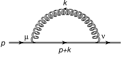
Figure 15: One-loop self-energy Feynman diagram for the propagation of a quark of momentum $p$ and bare mass $m_{b}$, and a gluon of mass $\lambda$.

The one-loop self energy, depicted in Fig. 15, for a quark with bare mass $m_{b}$, due to the exchange of a gluon of mass $\lambda$, computed in $d=4-2\epsilon$ dimensions, with $\mu$ rescaled according to the $\overline{\rm MS}$ prescription, is

$$\Sigma^{(1)}_{\lambda}(\not{p},m_{b},\mu,\alpha_{\mathchoice{\displaystyle}{\scriptstyle}{\scriptscriptstyle}{\scriptscriptstyle}\rm S}) = 4\pi\alpha_{\mathchoice{\displaystyle}{\scriptstyle}{\scriptscriptstyle}{\scriptscriptstyle}\rm S}\!\left(\frac{\mu^{2}e^{\gamma_{E}}}{4\pi}\right)^{\epsilon}\!\!\!\int\!\frac{\mathrm{d}^{d}k}{(2\pi)^{d}}(-i\gamma^{\nu}t^{a})\frac{i}{\not{p}+\not{k}-m_{b}+i\eta}(-i\gamma^{\mu}t^{a})\frac{-ig_{\mu\nu}}{k^{2}-\lambda^{2}+i\eta}$$ (115)

$$\equiv 4\pi\alpha_{\mathchoice{\displaystyle}{\scriptstyle}{\scriptscriptstyle}{\scriptscriptstyle}\rm S}\,C_{\mathchoice{\displaystyle}{\scriptstyle}{\scriptscriptstyle}{\scriptscriptstyle}\rm F}\,i\left[\mathcal{A}_{\lambda}\!\left(m_{b},\mu\right)\not{p}-\mathcal{B}_{\lambda}\!\left(m_{b},\mu\right)m_{b}\right],$$

where we assume $p^{2}=m_{b}^{2}$, and we have defined

$$\mathcal{A}_{\lambda}\!\left(m_{b},\mu\right) = -\frac{(2-d)}{2im_{b}^{2}}\left(\frac{\mu^{2}e^{\gamma_{E}}}{4\pi}\right)^{\epsilon}\left\{\int\frac{\mathrm{d}^{d}k}{(2\pi)^{d}}\frac{p^{2}-\lambda^{2}+m_{b}^{2}}{\left[(p+k)^{2}-m_{b}^{2}+i\eta\right]\left[k^{2}-\lambda^{2}+i\eta\right]}\right.$$ (116)

$$+\left.\int\frac{\mathrm{d}^{d}k}{(2\pi)^{d}}\frac{1}{k^{2}-\lambda^{2}+i\eta}-\int\frac{\mathrm{d}^{d}k}{(2\pi)^{d}}\frac{1}{k^{2}-m_{b}^{2}+i\eta}\right\},$$

$$\mathcal{B}_{\lambda}\!\left(m_{b},\mu\right) = \frac{d}{i}\left(\frac{\mu^{2}e^{\gamma_{E}}}{4\pi}\right)^{\epsilon}\int\frac{\mathrm{d}^{d}k}{(2\pi)^{d}}\frac{1}{\left[(p+k)^{2}-m_{b}^{2}+i\eta\right]\left[k^{2}-\lambda^{2}+i\eta\right]}\,.$$ (117)

The dressed quark propagator at one loop then reads

$$\frac{i}{\not{p}-m_{b}}+\frac{i}{\not{p}-m_{b}}\Sigma^{(1)}_{k}(\not{p},m_{b},\mu,\alpha_{\mathchoice{\displaystyle}{\scriptstyle}{\scriptscriptstyle}{\scriptscriptstyle}\rm S})\frac{i}{\not{p}-m_{b}}$$

$$\hskip 56.9055pt=\frac{i}{\not{p}-m_{b}}\left\{1-4\pi\alpha_{\mathchoice{\displaystyle}{\scriptstyle}{\scriptscriptstyle}{\scriptscriptstyle}\rm S}C_{\mathchoice{\displaystyle}{\scriptstyle}{\scriptscriptstyle}{\scriptscriptstyle}\rm F}\left[\mathcal{A}_{\lambda}\left(m_{b},\mu\right)\not{p}-\mathcal{B}_{\lambda}\left(m_{b},\mu\right)\,m_{b}\right]\frac{1}{\not{p}-m_{b}}\right\}$$

$$\hskip 56.9055pt=\frac{i\left[1+4\pi\alpha_{\mathchoice{\displaystyle}{\scriptstyle}{\scriptscriptstyle}{\scriptscriptstyle}\rm S}C_{\mathchoice{\displaystyle}{\scriptstyle}{\scriptscriptstyle}{\scriptscriptstyle}\rm F}\,\mathcal{A}_{\lambda}\left(m_{b},\mu\right)\right]^{-1}}{\not{p}-m_{b}\left\{1++4\pi\alpha_{\mathchoice{\displaystyle}{\scriptstyle}{\scriptscriptstyle}{\scriptscriptstyle}\rm S}C_{\mathchoice{\displaystyle}{\scriptstyle}{\scriptscriptstyle}{\scriptscriptstyle}\rm F}\left[\mathcal{B}_{\lambda}\left(m_{b},\mu\right)-\mathcal{A}_{\lambda}\left(m_{b},\mu\right)\right]\right\}}+\mathcal{O}\left(\alpha_{\mathchoice{\displaystyle}{\scriptstyle}{\scriptscriptstyle}{\scriptscriptstyle}\rm S}^{2}\right).\phantom{aaa}$$ (118)

The position of the pole in the propagator defines the pole mass

$$m\equiv m_{b}\left\{1+4\pi\alpha_{\mathchoice{\displaystyle}{\scriptstyle}{\scriptscriptstyle}{\scriptscriptstyle}\rm S}C_{\mathchoice{\displaystyle}{\scriptstyle}{\scriptscriptstyle}{\scriptscriptstyle}\rm F}\left[\mathcal{B}_{\lambda}\left(m_{b},\mu\right)-\mathcal{A}_{\lambda}\left(m_{b},\mu\right)\right]\right\}.$$ (119)

Neglecting terms of the order $\alpha_{\mathchoice{\displaystyle}{\scriptstyle}{\scriptscriptstyle}{\scriptscriptstyle}\rm S}^{2}$, we can write

$$m=m_{b}\left[1+\alpha_{\mathchoice{\displaystyle}{\scriptstyle}{\scriptscriptstyle}{\scriptscriptstyle}\rm S}\,r_{\lambda}(m,\mu)\right]\,,$$ (120)

where we have defined

$$r_{\lambda}(m,\mu) \equiv 4\pi\,C_{\mathchoice{\displaystyle}{\scriptstyle}{\scriptscriptstyle}{\scriptscriptstyle}\rm F}\left[\mathcal{B}_{\lambda}\left(m,\mu\right)-\mathcal{A}_{\lambda}\left(m,\mu\right)\right].$$ (121)

Furthermore, separating the finite and divergent part of $r_{\lambda}$ according to the $\overline{\rm MS}$ prescription

$$r_{\lambda}(m,\mu)=\frac{1}{\epsilon}r^{\rm(d)}_{\lambda}(m,\mu)+r^{\rm(f)}_{\lambda}(m,\mu)+{\cal O}(\epsilon),$$ (122)

we have that the $\overline{\rm MS}$ mass is given by

$$\overline{m}(\mu)=m_{b}\left[1+\alpha_{\mathchoice{\displaystyle}{\scriptstyle}{\scriptscriptstyle}{\scriptscriptstyle}\rm S}\frac{1}{\epsilon}r^{\rm(d)}_{\lambda}\left(\overline{m}(\mu),\mu\right)\right],$$ (123)

so that the relation between the pole mass and the $\overline{\rm MS}$ mass is

$$\overline{m}(\mu)=m\left[1-\alpha_{\mathchoice{\displaystyle}{\scriptstyle}{\scriptscriptstyle}{\scriptscriptstyle}\rm S}\,r^{(\rm f)}_{\lambda}\left(m,\mu\right)\right].$$ (124)

For a generic $\lambda$ value we have

$$\mathcal{A}_{\lambda}(m,\mu) = \frac{1}{(4\pi)^{2}}\left\{\frac{1}{\epsilon}+2-\log\frac{m^{2}}{\mu^{2}}-x(1+\log x)+(2-x)H(x)\right\}+{\cal O}(\epsilon)\,,$$ (125)

$$\mathcal{B}_{\lambda}(m,\mu) = \frac{1}{(4\pi)^{2}}\left\{\frac{4}{\epsilon}+6-4\log\frac{m^{2}}{\mu^{2}}+4H(x)\right\}+{\cal O}(\epsilon)\,,$$ (126)

where

$$x=\frac{\lambda^{2}}{m^{2}}$$ (127)

and

$$H(x)=\left\{\begin{array}[]{ll}\displaystyle{-\frac{x}{2}\log{x}-\sqrt{x(4-x)}\,\arctan\sqrt{\frac{4-x}{x}}}&x<4\,,\\[5.69054pt] \displaystyle{-\frac{x}{2}\,\log{x}+\frac{1}{2}\sqrt{x(x-4)}\log\frac{\sqrt{x}+\sqrt{x-4}}{\sqrt{x}-\sqrt{x-4}}}&x>4\,.\end{array}\right.$$ (128)

This leads to

$$r_{\lambda}(m,\mu)=\frac{C_{\mathchoice{\displaystyle}{\scriptstyle}{\scriptscriptstyle}{\scriptscriptstyle}\rm F}}{4\pi}\left\{\frac{3}{\epsilon}+4-3\log\frac{m^{2}}{\mu^{2}}+x(1+\log x)+(2+x)H(x)\right\}.$$ (129)

Our result is consistent with Ref. Ball:1995ni . Notice that, for large $\lambda$, eq. (129) becomes

$$r_{\lambda}(m,\mu)=\frac{C_{\mathchoice{\displaystyle}{\scriptstyle}{\scriptscriptstyle}{\scriptscriptstyle}\rm F}}{4\pi}\left\{\frac{3}{\epsilon}+\frac{5}{2}-3\log\frac{\lambda^{2}}{\mu^{2}}+\ldots\right\},$$ (130)

and for small $\lambda$

$$r_{\lambda}(m,\mu)=\frac{C_{\mathchoice{\displaystyle}{\scriptstyle}{\scriptscriptstyle}{\scriptscriptstyle}\rm F}}{4\pi}\left\{\frac{3}{\epsilon}+4-3\log\frac{m^{2}}{\mu^{2}}-2\pi\frac{\lambda}{m}+\ldots\right\}.$$ (131)

We also need the exact $d$-dimensional expression of $r_{\lambda}(m,\mu)$, for $\lambda=0$ and $\lambda\gg m$. For $\lambda=0$ we have

$$\mathcal{A}_{\lambda}^{0}(m,\mu) = \frac{1}{(4\pi)^{2}}\,e^{\epsilon{\gamma_{\mathchoice{\displaystyle}{\scriptstyle}{\scriptscriptstyle}{\scriptscriptstyle}E}}}\,\frac{\Gamma(1+\epsilon)}{\epsilon}\,\left(\frac{\mu^{2}}{m^{2}}\right)^{\epsilon}\frac{1}{1-2\epsilon}\,,$$ (132)

$$\mathcal{B}_{\lambda}^{0}(m,\mu) = \frac{1}{(4\pi)^{2}}\,e^{\epsilon{\gamma_{\mathchoice{\displaystyle}{\scriptstyle}{\scriptscriptstyle}{\scriptscriptstyle}E}}}\,\frac{\Gamma(1+\epsilon)}{\epsilon}\,\left(\frac{\mu^{2}}{m^{2}}\right)^{\epsilon}\frac{4-2\epsilon}{1-2\epsilon}\,,$$ (133)

$$r_{\lambda}^{0}(m,\mu) = \frac{C_{\mathchoice{\displaystyle}{\scriptstyle}{\scriptscriptstyle}{\scriptscriptstyle}\rm F}}{4\pi}\,e^{\epsilon{\gamma_{\mathchoice{\displaystyle}{\scriptstyle}{\scriptscriptstyle}{\scriptscriptstyle}E}}}\,\frac{\Gamma(1+\epsilon)}{\epsilon}\!\left(\frac{\mu^{2}}{m^{2}}\right)^{\epsilon}\frac{3-2\epsilon}{1-2\epsilon}.$$ (134)

For $\lambda\gg m$ (and $\mu\approx\lambda$) we have

$$\mathcal{A}^{\infty}_{\lambda}(\mu) \equiv \lim_{m\to 0}\mathcal{A}_{\lambda}(m,\mu)=\frac{1}{(4\pi)^{2}}\,e^{\epsilon{\gamma_{\mathchoice{\displaystyle}{\scriptstyle}{\scriptscriptstyle}{\scriptscriptstyle}E}}}\,\frac{\Gamma(1+\epsilon)}{\epsilon}\,\left(\frac{\mu^{2}}{\lambda^{2}}\right)^{\epsilon}\frac{2-2\epsilon}{2-\epsilon}\,,$$ (135)

$$\mathcal{B}^{\infty}_{\lambda}(\mu) \equiv \lim_{m\to 0}\mathcal{B}_{\lambda}(m,\mu)=\frac{1}{(4\pi)^{2}}\,e^{\epsilon{\gamma_{\mathchoice{\displaystyle}{\scriptstyle}{\scriptscriptstyle}{\scriptscriptstyle}E}}}\,\frac{\Gamma(1+\epsilon)}{\epsilon}\,\left(\frac{\mu^{2}}{\lambda^{2}}\right)^{\epsilon}\frac{4-2\epsilon}{1-\epsilon}\,,$$ (136)

$$r_{\lambda}^{\infty}(\mu) \equiv \lim_{m\to 0}r_{\lambda}(m,\mu)=\frac{C_{\mathchoice{\displaystyle}{\scriptstyle}{\scriptscriptstyle}{\scriptscriptstyle}\rm F}}{4\pi}\,e^{\epsilon{\gamma_{\mathchoice{\displaystyle}{\scriptstyle}{\scriptscriptstyle}{\scriptscriptstyle}E}}}\,\frac{\Gamma(1+\epsilon)}{\epsilon}\,\left(\frac{\mu^{2}}{\lambda^{2}}\right)^{\epsilon}\frac{2(3-2\epsilon)}{(1-\epsilon)(2-\epsilon)}.$$ (137)

C.2 All-orders result

In this section we deal with the computation of the on-shell top self-energy in $d=4-2\epsilon$ dimensions, $\Sigma(\not{p},m_{b},\mu,\alpha_{\mathchoice{\displaystyle}{\scriptstyle}{\scriptscriptstyle}{\scriptscriptstyle}\rm S})$, with the insertion of an infinite number of light-quark loops in the gluon line. The one-loop self energy with a massless gluon is obtained by setting $\lambda=0$ in eq. (115). According to App. A, once the gluon line is dressed with all possible light-quark loop insertions, the expression for the self-energy becomes

$$\Sigma(\not{p},m_{b},\mu,\alpha_{\mathchoice{\displaystyle}{\scriptstyle}{\scriptscriptstyle}{\scriptscriptstyle}\rm S}) = 4\,\pi\,\alpha_{\mathchoice{\displaystyle}{\scriptstyle}{\scriptscriptstyle}{\scriptscriptstyle}\rm S}\left(\frac{\mu^{2}e^{\gamma_{E}}}{4\pi}\right)^{\epsilon}\int\frac{\mathrm{d}^{d}k}{(2\pi)^{d}}(-i\gamma^{\nu}t^{a})\frac{i}{\not{p}+\not{k}-m_{b}}(-i\gamma^{\mu}t^{a})$$ (138)

$$\hskip 85.35826pt\times\frac{-ig_{\mu\nu}}{(k^{2}+i\eta)[1+\Pi(k^{2},\mu^{2})-\Pi_{\rm ct}]}$$

$$\equiv 4\pi\alpha_{\mathchoice{\displaystyle}{\scriptstyle}{\scriptscriptstyle}{\scriptscriptstyle}\rm S}\,C_{\mathchoice{\displaystyle}{\scriptstyle}{\scriptscriptstyle}{\scriptscriptstyle}\rm F}\,i\left[\mathcal{A}\!\left(m_{b},\mu\right)\not{p}-\mathcal{B}\!\left(m_{b},\mu\right)m_{b}\right],$$

where we assume $p^{2}=m_{b}^{2}$ and the $\overline{\rm MS}$ scheme expressions of $\Pi$ and $\Pi_{\rm ct}$ are given by eqs. (64) and (66), respectively. Using eq. (97) we can rewrite eq. (138) as

$${\Sigma}(\not{p},m_{b},\mu,\alpha_{\mathchoice{\displaystyle}{\scriptstyle}{\scriptscriptstyle}{\scriptscriptstyle}\rm S})=-\frac{1}{\pi}\int_{0-}^{\infty}\mathrm{d}\lambda^{2}\,\,\Sigma_{\lambda}^{(1)}\!\left(\not{p},m_{b},\mu,\alpha_{\mathchoice{\displaystyle}{\scriptstyle}{\scriptscriptstyle}{\scriptscriptstyle}\rm S}\right)\,{\rm Im}\left[\frac{1}{\lambda^{2}+i\eta}\,\frac{1}{1+\Pi(\lambda^{2},\mu^{2})-\Pi_{\rm ct}}\right],$$ (139)

where $\Sigma_{\lambda}^{(1)}$ is defined in eq. (115). Defining as before the function $r$ such that

$$m=m_{b}\left[1+\alpha_{\mathchoice{\displaystyle}{\scriptstyle}{\scriptscriptstyle}{\scriptscriptstyle}\rm S}\,r(m,\mu,\alpha_{\mathchoice{\displaystyle}{\scriptstyle}{\scriptscriptstyle}{\scriptscriptstyle}\rm S})\right]+\mathcal{O}\!\left(\alpha_{\mathchoice{\displaystyle}{\scriptstyle}{\scriptscriptstyle}{\scriptscriptstyle}\rm S}^{2}\left(\alpha_{\mathchoice{\displaystyle}{\scriptstyle}{\scriptscriptstyle}{\scriptscriptstyle}\rm S}b_{0}\right)^{n}\right)$$ (140)

is the pole mass position, we get

$$r(m,\mu,\alpha_{\mathchoice{\displaystyle}{\scriptstyle}{\scriptscriptstyle}{\scriptscriptstyle}\rm S}) = -\frac{1}{\pi}\int_{0-}^{\infty}\mathrm{d}\lambda^{2}\hskip 1.69998ptr_{\lambda}(m,\mu)\,\mathrm{{\rm Im}}\left[\frac{1}{\lambda^{2}+i\eta}\hskip 1.69998pt\frac{1}{1+\Pi(\lambda^{2},\mu^{2})-\Pi_{\rm ct}}\right].$$ (141)

In analogy with eq. (124), we can write

$$\overline{m}(\mu)=m\left[1-\alpha_{\mathchoice{\displaystyle}{\scriptstyle}{\scriptscriptstyle}{\scriptscriptstyle}\rm S}\,r^{\rm(f)}(m,\mu,\alpha_{\mathchoice{\displaystyle}{\scriptstyle}{\scriptscriptstyle}{\scriptscriptstyle}\rm S})\right]+\mathcal{O}(\alpha_{\mathchoice{\displaystyle}{\scriptstyle}{\scriptscriptstyle}{\scriptscriptstyle}\rm S}^{2}(\alpha_{\mathchoice{\displaystyle}{\scriptstyle}{\scriptscriptstyle}{\scriptscriptstyle}\rm S}b_{0})^{n}),$$ (142)

where $r^{\rm(f)}(m,\mu,\alpha_{\mathchoice{\displaystyle}{\scriptstyle}{\scriptscriptstyle}{\scriptscriptstyle}\rm S})$ denotes the finite part (according to the $\overline{\rm MS}$ scheme) of $r(m,\mu,\alpha_{\mathchoice{\displaystyle}{\scriptstyle}{\scriptscriptstyle}{\scriptscriptstyle}\rm S})$.

In order to compute eq. (141), since $r_{\lambda}$ contains a single pole in $\epsilon$ and does not go to zero for large $\lambda$, besides its value given in eq. (121), we need its value for $\lambda=0$ and its asymptotic value for large $\lambda$ in $d=4-2\epsilon$ dimensions at all orders in $\epsilon$. Their expressions are given in eqs. (134) and (137) respectively. We also express $r_{\lambda}$ as the sum of following two terms

$$r_{\lambda,d}\!\left(m,\mu\right) = \frac{\mu^{2}}{\mu^{2}+\lambda^{2}}\,r_{\lambda}^{0}(m,\mu)+\frac{\lambda^{2}}{\mu^{2}+\lambda^{2}}\,r_{\lambda}^{\infty}\!\left(\mu\right),$$ (143)

$$r_{\lambda,f}\!\left(m,\mu\right) = r_{\lambda}\!\left(m,\mu\right)-r_{\lambda,d}\!\left(m,\mu\right)$$ (144)

and we write

$$r(m,\mu,\alpha_{\mathchoice{\displaystyle}{\scriptstyle}{\scriptscriptstyle}{\scriptscriptstyle}\rm S}) = r_{f}(m,\mu,\alpha_{\mathchoice{\displaystyle}{\scriptstyle}{\scriptscriptstyle}{\scriptscriptstyle}\rm S})+r_{d}(m,\mu,\alpha_{\mathchoice{\displaystyle}{\scriptstyle}{\scriptscriptstyle}{\scriptscriptstyle}\rm S})\,,$$ (145)

$$r_{f}(m,\mu,\alpha_{\mathchoice{\displaystyle}{\scriptstyle}{\scriptscriptstyle}{\scriptscriptstyle}\rm S}) \equiv -\frac{1}{\pi}\int_{0-}^{\infty}\mathrm{d}\lambda^{2}\,r_{\lambda,f}\!\left(m,\mu\right){\rm Im}\left[\frac{1}{\lambda^{2}+i\eta}\,\frac{1}{1+\Pi(\lambda^{2},\mu^{2})-\Pi_{\rm ct}}\right],$$ (146)

$$r_{d}(m,\mu,\alpha_{\mathchoice{\displaystyle}{\scriptstyle}{\scriptscriptstyle}{\scriptscriptstyle}\rm S}) \equiv -\frac{1}{\pi}\int_{0-}^{\infty}\mathrm{d}\lambda^{2}\,r_{\lambda,d}\!\left(m,\mu\right){\rm Im}\left[\frac{1}{\lambda^{2}+i\eta}\,\frac{1}{1+\Pi(\lambda^{2},\mu^{2})-\Pi_{\rm ct}}\right].$$ (147)

The function $r_{\lambda,f}(m,\mu)$ vanishes for $\lambda^{2}\to 0$ and for $\lambda^{2}\to\infty$. In addition, it has a finite limit for $\epsilon\to 0$, so that we can write

$$r_{\lambda,f}\!\left(m,\mu\right) = \frac{C_{\mathchoice{\displaystyle}{\scriptstyle}{\scriptscriptstyle}{\scriptscriptstyle}\rm F}}{4\pi}\left\{-3\log\!\left(\frac{m^{2}}{\mu^{2}}\right)+\frac{\lambda^{2}}{m^{2}}\left(1+\log\frac{\lambda^{2}}{m^{2}}\right)+4+\left(2+\frac{\lambda^{2}}{m^{2}}\right)H\left(\frac{\lambda^{2}}{m^{2}}\right)\right.$$ (148)

$$- \left.\!\frac{\mu^{2}}{\mu^{2}+\lambda^{2}}\,\left[-3\log\!\left(\frac{m^{2}}{\mu^{2}}\right)+4\right]-\frac{\lambda^{2}}{\mu^{2}+\lambda^{2}}\,\left[-3\log\!\left(\frac{\lambda^{2}}{\mu^{2}}\right)+\frac{5}{2}\right]\right\}+{\cal O}(\epsilon)\,.\phantom{aaaaaa}$$

For these reasons, we can manipulate $r_{f}(m,\mu,\alpha_{\mathchoice{\displaystyle}{\scriptstyle}{\scriptscriptstyle}{\scriptscriptstyle}\rm S})$ according to the same procedure used in App. B, to get

$$r_{f}(m,\mu,\alpha_{\mathchoice{\displaystyle}{\scriptstyle}{\scriptscriptstyle}{\scriptscriptstyle}\rm S}) = -\frac{3\pi}{\alpha_{\mathchoice{\displaystyle}{\scriptstyle}{\scriptscriptstyle}{\scriptscriptstyle}\rm S}T_{\mathchoice{\displaystyle}{\scriptstyle}{\scriptscriptstyle}{\scriptscriptstyle}\rm F}}\int_{0}^{\infty}\frac{\mathrm{d}\lambda}{\pi}\,\frac{\mathrm{d}\ }{\mathrm{d}\lambda}\left[r_{\lambda,f}\!\left(m,\mu\right)\right]{\rm Im}\left\{\log\left[1+\Pi\left(\lambda^{2},\mu^{2}\right)-\Pi_{\rm ct}\right]\right\},$$ (149)

$$= -\frac{1}{b_{0}\,\alpha_{\mathchoice{\displaystyle}{\scriptstyle}{\scriptscriptstyle}{\scriptscriptstyle}\rm S}}\int_{0}^{\infty}\frac{\mathrm{d}\lambda}{\pi}\,\frac{\mathrm{d}\ }{\mathrm{d}\lambda}\left[r_{\lambda,f}\!\left(m,\mu\right)\right]\arctan\frac{\pi\,b_{0}\,\alpha_{\mathchoice{\displaystyle}{\scriptstyle}{\scriptscriptstyle}{\scriptscriptstyle}\rm S}}{1+b_{0}\,\alpha_{\mathchoice{\displaystyle}{\scriptstyle}{\scriptscriptstyle}{\scriptscriptstyle}\rm S}\log\displaystyle{\frac{\lambda^{2}}{\mu_{\mathchoice{\displaystyle}{\scriptstyle}{\scriptscriptstyle}{\scriptscriptstyle}C}^{2}}}}\,,$$

that can be evaluated numerically. We notice that $r_{f}(m,\mu,\alpha_{\mathchoice{\displaystyle}{\scriptstyle}{\scriptscriptstyle}{\scriptscriptstyle}\rm S})$ contains a linear infrared renormalon, since the behaviour of $r_{\lambda,f}\!\left(m,\mu\right)$ for small $\lambda$ is

$$r_{\lambda,f}\!\left(m,\mu\right)\approx-\frac{C_{\mathchoice{\displaystyle}{\scriptstyle}{\scriptscriptstyle}{\scriptscriptstyle}\rm F}}{2}\frac{\lambda}{m}\,.$$ (150)

As far as the integral in eq. (147) is concerned, we can split it into two terms, according to eq. (143),

$$r_{d}(m,\mu,\alpha_{\mathchoice{\displaystyle}{\scriptstyle}{\scriptscriptstyle}{\scriptscriptstyle}\rm S}) = r_{d}^{0}(m,\mu,\alpha_{\mathchoice{\displaystyle}{\scriptstyle}{\scriptscriptstyle}{\scriptscriptstyle}\rm S})+r_{d}^{\infty}(m,\mu,\alpha_{\mathchoice{\displaystyle}{\scriptstyle}{\scriptscriptstyle}{\scriptscriptstyle}\rm S})\,,$$ (151)

$$r_{d}^{0}(m,\mu,\alpha_{\mathchoice{\displaystyle}{\scriptstyle}{\scriptscriptstyle}{\scriptscriptstyle}\rm S}) \equiv -\frac{1}{\pi}\int_{0-}^{\infty}\!\mathrm{d}\lambda^{2}\,\frac{\mu^{2}}{\mu^{2}+\lambda^{2}}\,r_{\lambda}^{0}(m,\mu)\,{\rm Im}\left[\frac{1}{\lambda^{2}+i\eta}\,\frac{1}{1+\Pi(\lambda^{2},\mu^{2})-\Pi_{\rm ct}}\right]\!,\phantom{aaa}$$ (152)

$$r_{d}^{\infty}(m,\mu,\alpha_{\mathchoice{\displaystyle}{\scriptstyle}{\scriptscriptstyle}{\scriptscriptstyle}\rm S}) \equiv -\frac{1}{\pi}\int_{0-}^{\infty}\!\mathrm{d}\lambda^{2}\,\frac{\lambda^{2}}{\mu^{2}+\lambda^{2}}\,r^{\infty}_{\lambda}(\mu)\,{\rm Im}\left[\frac{1}{\lambda^{2}+i\eta}\,\frac{1}{1+\Pi(\lambda^{2},\mu^{2})-\Pi_{\rm ct}}\right]\!.\phantom{aaaaa}$$ (153)

Using eq. (97), we can write

$$r_{d}^{0}(m,\mu,\alpha_{\mathchoice{\displaystyle}{\scriptstyle}{\scriptscriptstyle}{\scriptscriptstyle}\rm S})=r_{\lambda}^{0}(m,\mu)\,\frac{1}{1+\Pi(-\mu^{2},\mu^{2})-\Pi_{\rm ct}}.$$ (154)

In order to deal with the integral in $r_{d}^{\infty}(m,\mu,\alpha_{\mathchoice{\displaystyle}{\scriptstyle}{\scriptscriptstyle}{\scriptscriptstyle}\rm S})$, we need to expose the $\lambda$ dependence of the integrand. From eq. (137), we can write

$$r^{\infty}_{\lambda}(\mu)=\left(\frac{\lambda^{2}}{\mu^{2}}\right)^{-\epsilon}R^{\infty},$$ (155)

where $R^{\infty}$ depends only on $\epsilon$ and no longer on $\lambda$. Similarly, using eq. (64), we have

$$\Pi\left(\lambda^{2},\mu^{2}\right) = \frac{\alpha_{\mathchoice{\displaystyle}{\scriptstyle}{\scriptscriptstyle}{\scriptscriptstyle}\rm S}T_{\mathchoice{\displaystyle}{\scriptstyle}{\scriptscriptstyle}{\scriptscriptstyle}\rm F}}{\pi}e^{\epsilon{\gamma_{\mathchoice{\displaystyle}{\scriptstyle}{\scriptscriptstyle}{\scriptscriptstyle}E}}}\frac{\Gamma(1+\epsilon)\,\Gamma^{2}(1-\epsilon)}{\Gamma(1-2\epsilon)}\frac{1-\epsilon}{(3-2\epsilon)(1-2\epsilon)}\,\frac{1}{\epsilon}\left(\frac{\lambda^{2}}{\mu^{2}}\right)^{-\epsilon}e^{i\epsilon\pi}$$ (156)

$$= \Pi\left(-\mu^{2},\mu^{2}\right)\left(\frac{\lambda^{2}}{\mu^{2}}\right)^{-\epsilon}e^{i\epsilon\pi},$$

and we can write

$$r_{d}^{\infty}(m,\mu,\alpha_{\mathchoice{\displaystyle}{\scriptstyle}{\scriptscriptstyle}{\scriptscriptstyle}\rm S}) = -\frac{R^{\infty}}{\pi}\int_{0}^{\infty}\mathrm{d}\lambda^{2}\,\frac{1}{\mu^{2}+\lambda^{2}}\left(\frac{\lambda^{2}}{\mu^{2}}\right)^{-\epsilon}\,{\rm Im}\left[\frac{1}{1+\Pi(\lambda^{2},\mu^{2})-\Pi_{\rm ct}}\right]$$ (157)

$$= -\frac{R^{\infty}}{\pi}\,\sum_{n=0}^{\infty}\,(-1)^{n}\int_{0}^{\infty}\mathrm{d}\lambda^{2}\,\frac{1}{\mu^{2}+\lambda^{2}}\left(\frac{\lambda^{2}}{\mu^{2}}\right)^{-\epsilon}$$

$$\hskip 85.35826pt\times\,{\rm Im}\left[\Pi\left(-\mu^{2},\mu^{2}\right)\left(\frac{\lambda^{2}}{\mu^{2}}\right)^{-\epsilon}e^{i\epsilon\pi}-\Pi_{\rm ct}\right]^{n}$$

$$= -\frac{R^{\infty}}{\pi}\,\sum_{n=0}^{\infty}\,(-1)^{n}\int_{0}^{\infty}\mathrm{d}z\,\frac{z^{-\epsilon}}{1+z}\,{\rm Im}\left[\Pi\left(-\mu^{2},\mu^{2}\right)z^{-\epsilon}e^{i\epsilon\pi}-\Pi_{\rm ct}\right]^{n},\phantom{aaa}$$

where we have performed a Taylor expansion in the second line. By computing the imaginary part of the $n$-th power of the term in the square brackets, we are lead to evaluate integrals of the form

$$\int_{0}^{\infty}\mathrm{d}z\,\frac{z^{-h}}{1+z}=\Gamma(1-h)\,\Gamma(h),$$ (158)

where $h$ is a real number, so that $r_{d}^{\infty}(m,\mu,\alpha_{\mathchoice{\displaystyle}{\scriptstyle}{\scriptscriptstyle}{\scriptscriptstyle}\rm S})$ can be straightforwardly evaluated by computer algebraic means at any fixed order in $\alpha_{\mathchoice{\displaystyle}{\scriptstyle}{\scriptscriptstyle}{\scriptscriptstyle}\rm S}$.

We emphasize that $r_{d}(m,\mu,\alpha_{\mathchoice{\displaystyle}{\scriptstyle}{\scriptscriptstyle}{\scriptscriptstyle}\rm S})$ has no linear renormalon. Indeed if we perform an $\epsilon$ expansion and we consider the small $\lambda$ contribution, by writing $\mathrm{d}\lambda^{2}=2\lambda\mathrm{d}\lambda$, we notice that the integrand behaves as $\lambda\log^{n}(\lambda)$. This signals the absence of linear renormalons, that come from terms of the type $\log^{n}(\lambda)$, without any power of $\lambda$ in front.

From eq. (142) we get

$$\overline{m}(\mu)=m\left\{1-\alpha_{\mathchoice{\displaystyle}{\scriptstyle}{\scriptscriptstyle}{\scriptscriptstyle}\rm S}\left[r_{f}(m,\mu,\alpha_{\mathchoice{\displaystyle}{\scriptstyle}{\scriptscriptstyle}{\scriptscriptstyle}\rm S})+r_{d}^{\rm(f)}(m,\mu,\alpha_{\mathchoice{\displaystyle}{\scriptstyle}{\scriptscriptstyle}{\scriptscriptstyle}\rm S})\right]\right\}+\mathcal{O}\!\left(\alpha_{\mathchoice{\displaystyle}{\scriptstyle}{\scriptscriptstyle}{\scriptscriptstyle}\rm S}^{2}(\alpha_{\mathchoice{\displaystyle}{\scriptstyle}{\scriptscriptstyle}{\scriptscriptstyle}\rm S}b_{0})^{n}\right),$$ (159)

where $r_{d}^{\rm(f)}$ is the finite part (according to the $\overline{\rm MS}$ scheme) of $r_{d}$. If we expand $\left(r_{f}+r_{d}^{\rm(f)}\right)$ is series of $\alpha_{\mathchoice{\displaystyle}{\scriptstyle}{\scriptscriptstyle}{\scriptscriptstyle}\rm S}$

$$r^{\rm(f)}(m,\mu,\alpha_{\mathchoice{\displaystyle}{\scriptstyle}{\scriptscriptstyle}{\scriptscriptstyle}\rm S})=r_{f}(m,\mu,\alpha_{\mathchoice{\displaystyle}{\scriptstyle}{\scriptscriptstyle}{\scriptscriptstyle}\rm S})+r_{d}^{\rm(f)}(m,\mu,\alpha_{\mathchoice{\displaystyle}{\scriptstyle}{\scriptscriptstyle}{\scriptscriptstyle}\rm S})\equiv\sum_{i=0}^{\infty}c_{i+1}(m,\mu)\,\alpha_{\mathchoice{\displaystyle}{\scriptstyle}{\scriptscriptstyle}{\scriptscriptstyle}\rm S}^{i},$$ (160)

we obtain

$$\overline{m}(\mu)=m\left[1-\,\,\sum_{i=1}^{\infty}c_{i}(m,\mu)\,\alpha_{\mathchoice{\displaystyle}{\scriptstyle}{\scriptscriptstyle}{\scriptscriptstyle}\rm S}^{i}\right]+\mathcal{O}\!\left(\alpha_{\mathchoice{\displaystyle}{\scriptstyle}{\scriptscriptstyle}{\scriptscriptstyle}\rm S}^{2}\left(\alpha_{\mathchoice{\displaystyle}{\scriptstyle}{\scriptscriptstyle}{\scriptscriptstyle}\rm S}b_{0}\right)^{n}\right).$$ (161)

Appendix D Cancellation of the linear sensitivity in the total cross section and in “leptonic” observables

In order to discuss the issue of the linear sensitivity cancellation in the total cross section and in $E_{\mathchoice{\displaystyle}{\scriptstyle}{\scriptscriptstyle}{\scriptscriptstyle}W}$, it is convenient to use the old-fashioned perturbation theory. One writes the propagators as the sum of an advanced and retarded part

$$\frac{i}{k^{2}-m^{2}+i\eta} = \frac{i}{2E_{k,m}}\left[\frac{1}{k^{0}-E_{k,m}+i\eta}+\frac{1}{-k^{0}-E_{k,m}+i\eta}\right],$$ (162)

$$E_{k,m} = \sqrt{\vec{k}^{2}+m^{2}},$$ (163)

while, for unstable particles, we have

$$\frac{i}{k^{2}-m^{2}+im\Gamma} = \frac{i}{2E_{k,m,\Gamma}}\left[\frac{1}{k^{0}-E_{k,m,\Gamma}}+\frac{1}{-k^{0}-E_{k,m,\Gamma}}\right],$$ (164)

$$E_{k,m,\Gamma} = \sqrt{\underline{k}^{2}+m^{2}-im\Gamma}\,.$$ (165)

In this way, each Feynman graph is separated into contributions where the vertexes have all possible time orderings. Each line joining two vertexes has an energy set to its on-shell value, with an extra negative sign when considering a retarded propagator. For each time ordering the integration of all the $k^{0}$ components yields a product of old-fashioned perturbation theory denominators

$$D_{i}=\frac{1}{E-E_{i}+i\eta}\,,$$ (166)

where $E$ is the total energy and $E_{i}$ is the energy of the state $i$, given by the sum of the energies flowing in the $i^{\rm th}$ cut of the amplitude, times an overall delta function of energy conservation.

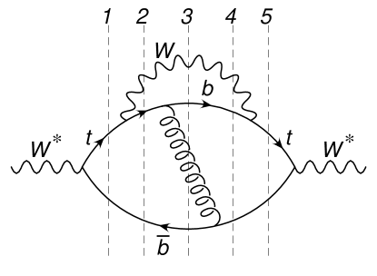
Figure 16: One time-ordered graph contributing to the $W^{*}\rightarrow t\bar{b}\to Wb\bar{b}$ cross section.

In Fig. 16 we show a possible time ordering for one graph contributing to the $W^{*}\rightarrow t\bar{b}\to Wb\bar{b}$ cross section. The corresponding contribution to the cross section is obtained by setting either one of the 2, 3, 4 intermediate states on the energy shell, and changing the sign of the $i\eta$ in the denominators to the right of the cut. We then define

$$D_{1} = \frac{1}{E-E_{t,1}-E_{\bar{b},1}}\,,$$ (167)

$$D_{2} = \frac{1}{E-E_{\mathchoice{\displaystyle}{\scriptstyle}{\scriptscriptstyle}{\scriptscriptstyle}W}-E_{b,2}-E_{\bar{b},1}+i\eta}\,,$$ (168)

$$D_{3} = \frac{1}{E-E_{\mathchoice{\displaystyle}{\scriptstyle}{\scriptscriptstyle}{\scriptscriptstyle}W}-E_{b,3}-E_{\bar{b},1}-E_{g,3}+i\eta}\,,$$ (169)

$$D_{4} = \frac{1}{E-E_{\mathchoice{\displaystyle}{\scriptstyle}{\scriptscriptstyle}{\scriptscriptstyle}W}-E_{b,3}-E_{\bar{b},4}+i\eta}\,,$$ (170)

$$D_{5} = \frac{1}{E-E_{t,5}-E_{\bar{b},5}}\,,$$ (171)

where

$$E_{t,i} = \sqrt{\vec{k}_{t,i}^{2}+m^{2}-im\Gamma_{t}}\,,$$ (172)

$$E_{l,i} = \sqrt{\vec{k}_{l,i}^{2}}\,,\qquad{\rm for}\qquad l=b,\,\bar{b},\,g,\,$$ (173)

$$E_{\mathchoice{\displaystyle}{\scriptstyle}{\scriptscriptstyle}{\scriptscriptstyle}W} = \sqrt{{\vec{k}^{2}_{\mathchoice{\displaystyle}{\scriptstyle}{\scriptscriptstyle}{\scriptscriptstyle}W}}+m^{2}}\,.$$ (174)

Notice that the top energy has an imaginary part, so that no $i\eta$ is needed in the denominators containing it. We never include the corresponding cuts since the top width prevents this particle from being on-shell. Thus, the only intermediate states contributing to cuts will be the ones that do not include the top. Then, in the integrand for the cross section, we have the sum

$$D_{1}\left[{\rm Im}\left(D_{2}\right)D_{3}^{*}\,D_{4}^{*}+D_{2}\,{\rm Im}\left(D_{3}\right)D_{4}^{*}+D_{2}\,D_{3}\,{\rm Im}\left(D_{4}\right)\right]D_{5}^{*}\,,$$ (175)

that is algebraically equal to $D_{1}\,{\rm Im}[D_{2}D_{3}D_{4}]D_{5}^{*}$. In fact

$$D_{1}\,{\rm Im}\left[D_{2}\,D_{3}\,D_{4}\right]D_{5}^{*}=\frac{1}{2i}D_{1}\left[D_{2}\,D_{3}\,D_{4}-\left(D_{2}\,D_{3}\,D_{4}\right)^{*}\right]D_{5}^{*}.$$ (176)

When performing the 3-momentum integral for the loops not including the $W$ line, one can approach the singularity in the denominator. However, if there is a direction in the 9-dimensional integration space (corresponding to the three 3-momenta flowing in the loops) such that, integrating along it, it leaves the singularities of $D_{2}$, $D_{3}$ and $D_{4}$ on the same side of the complex plane, the integration contour can be deformed away from the singularities, so that the denominators cannot contribute to mass singularities. The singularity for small gluon mass $m_{g}$ is thus determined only by the remaining factor

$$\frac{\mathrm{d}^{3}k_{g}}{\sqrt{\vec{k}_{g}^{2}+m_{g}^{2}}}\,,$$ (177)

that gives a quadratic sensitivity to the gluon mass. The only cases when an appropriate deformation of the contour does not exist correspond to Landau singularities Landau:1959fi . These are characterised by the presence of configurations with intermediate on-shell particles corresponding to classical propagation over large distances. It can be proven that the Landau singularities arise when several denominators go simultaneously on-shell and the momenta of the particles are such that they meet again after having come apart. If this is not possible, the singularity is an avoidable one.

In order to explore the possible Landau configurations, one can start with the graph of Fig. 16 with the top lines shrunk to a point. In fact, the top is always off-shell, and it cannot propagate over large distances. The remaining configuration is shown in Fig. 17.

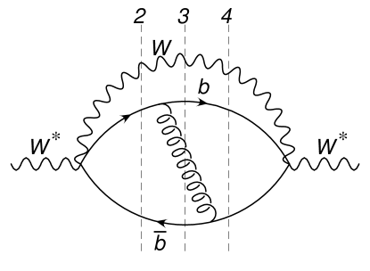
Figure 17: The reduced graph to look for Landau singularities in the graph of Fig. 16.

In order for the 2, 3 and 4 intermediate states to be on-shell at the same time, either both the $b$ and the $\bar{b}$ quarks should be collinear to the gluon, or the gluon should be soft. In the first case, also the $b$, the $\bar{b}$ and the gluon are collinear, and are all travelling in the opposite direction with respect to the $W$. Thus, they cannot meet at the same point on the last vertex to the right. On the other hand, if the gluon is soft, the $b$, the $\bar{b}$ and the $W$ produced at the primary vertex have momenta that sum to zero, so, again their velocities will make them diverge. One can try to shrink other propagators to a point. Shrinking one fermion propagator to a point, for example the $b$ one at the intermediate state 2, forces the gluon to be either collinear to the $\bar{b}$ or soft, and again one would end up with a $W$, a $b$ and a collinear $bg$ system produced at the vertex on the left and meeting at the vertex on the right, which is impossible. Shrinking the $W$, the two $b$ or the two $\bar{b}$ lines to a point shrinks the whole graph to a point, leading to nothing. Shrinking a $b$ and a $\bar{b}$ line to a point leads again to configuration with two massless system (either $b$ quarks of collinear $bg$ systems) and a $W$, that again cannot meet at the same point. Thus, no Landau configuration can exist, so one infers that the $m_{g}$ sensitivity of the total cross section is at least quadratic.

We can repeat the same reasoning including a factor $E_{\mathchoice{\displaystyle}{\scriptstyle}{\scriptscriptstyle}{\scriptscriptstyle}W}$ in our Feynman graph. The argument runs as before, and so, even for the average energy of the $W$ boson, one expects that the sensitivity to the gluon mass is at least quadratic. Notice that, in order for this to work, one needs that the $E_{\mathchoice{\displaystyle}{\scriptstyle}{\scriptscriptstyle}{\scriptscriptstyle}W}$ factor is the same for all cuts, which is in fact the case.

The argument fails if the top width is sent to zero. In fact, even at the Born level (i.e. removing the gluon line) the first and last intermediate states have equal energy, but their $i\eta$ have opposite signs. Under these condition, the pinch is clearly unavoidable.

As a last point, we recall that the total cross section is free of linear $m_{g}$ sensitivity also in the limit of zero width. This happens because, in the zero-width limit, the cross section factorizes into a production cross section times a decay width, and both of them are free of linear sensitivity to $m_{g}$ if the mass is in a short-distance scheme. The same, however, does not hold for the average $E_{\mathchoice{\displaystyle}{\scriptstyle}{\scriptscriptstyle}{\scriptscriptstyle}W}$. In fact, the cancellation of mass singularities in $\Gamma_{t}$ cannot be proven in the same fashion adopted here, since logarithmic divergences are also present in the wave-function renormalization, and cannot be treated in a straightforward way in the old-fashioned perturbation theory.

References

- (1) ATLAS collaboration, B. Pearson, Top quark mass in ATLAS, in 10th International Workshop on Top Quark Physics (TOP2017) Braga, Portugal, September 17-22, 2017, 2017, 1711.09763.
- (2) CMS collaboration, A. Castro, Recent Top Quark Mass Measurements from CMS, in 10th International Workshop on Top Quark Physics (TOP2017) Braga, Portugal, September 17-22, 2017, 2017, 1712.01027, http://inspirehep.net/record/1640641/files/arXiv:1712.01027.pdf.
- (3) ATLAS collaboration, M. Aaboud et al., Measurement of the top quark mass in the dilepton channel from TeV ATLAS data, Phys. Lett. B761 (2016) 350 [1606.02179].
- (4) CMS collaboration, V. Khachatryan et al., Measurement of the top quark mass using proton-proton data at = 7 and 8 TeV, Phys. Rev. D93 (2016) 072004 [1509.04044].
- (5) S. Ferrario Ravasio, T. Ježo, P. Nason and C. Oleari, A theoretical study of top-mass measurements at the LHC using NLO+PS generators of increasing accuracy, Eur. Phys. J. C78 (2018) 458 [1801.03944].
- (6) Hoang, André H. and Plätzer, Simon and Samitz, Daniel, On the Cutoff Dependence of the Quark Mass Parameter in Angular Ordered Parton Showers, 1807.06617.
- (7) D. J. Gross and A. Neveu, Dynamical Symmetry Breaking in Asymptotically Free Field Theories, Phys. Rev. D10 (1974) 3235.
- (8) B. E. Lautrup, On High Order Estimates in QED, Phys. Lett. 69B (1977) 109.
- (9) G. ’t Hooft, in: THE WHYS OF SUBNUCLEAR PHYSICS. PROCEEDINGS OF THE 1977 INTERNATIONAL SCHOOL OF SUBNUCLEAR PHYSICS, HELD IN ERICE, TRAPANI, SICILY, JULY 23 - AUGUST 10, 1977, editor A. Zichichi, New York, Usa: Plenum Pr.(1979) 1247 P.(The Subnuclear Series, Vol.15) (1979) .
- (10) G. Parisi, On Infrared Divergences, Nucl. Phys. B150 (1979) 163.
- (11) A. H. Mueller, On the Structure of Infrared Renormalons in Physical Processes at High-Energies, Nucl. Phys. B250 (1985) 327.
- (12) A. H. Mueller, The QCD perturbation series, in QCD 20 Years Later: Proceedings, Workshop, Aachen, Germany, June 9-13, 1992, pp. 162–171, 1992.
- (13) G. Altarelli, Introduction to renormalons, in 5th Hellenic School and Workshops on Elementary Particle Physics (CORFU 1995) Corfu, Greece, September 3-24, 1995, pp. 221–236, 1995, http://preprints.cern.ch/cgi-bin/setlink?base=preprint&categ=cern&id=th-95-309.
- (14) M. Beneke, Renormalons, Phys. Rept. 317 (1999) 1 [hep-ph/9807443].
- (15) M. Beneke and V. M. Braun, Naive nonabelianization and resummation of fermion bubble chains, Phys. Lett. B348 (1995) 513 [hep-ph/9411229].
- (16) Particle Data Group collaboration, C. Patrignani et al., Electroweak model and constraints on new physics, Review of Particle Physics, Chin. Phys. C40 (2016) 100001.
- (17) J. de Blas, M. Ciuchini, E. Franco, S. Mishima, M. Pierini, L. Reina et al., Electroweak precision observables and Higgs-boson signal strengths in the Standard Model and beyond: present and future, JHEP 12 (2016) 135 [1608.01509].
- (18) Gfitter Group collaboration, M. Baak, J. Cúth, J. Haller, A. Hoecker, R. Kogler, K. Mönig et al., The global electroweak fit at NNLO and prospects for the LHC and ILC, Eur. Phys. J. C74 (2014) 3046 [1407.3792].
- (19) G. Degrassi, S. Di Vita, J. Elias-Miro, J. R. Espinosa, G. F. Giudice, G. Isidori et al., Higgs mass and vacuum stability in the Standard Model at NNLO, JHEP 08 (2012) 098 [1205.6497].
- (20) D. Buttazzo, G. Degrassi, P. P. Giardino, G. F. Giudice, F. Sala, A. Salvio et al., Investigating the near-criticality of the Higgs boson, JHEP 12 (2013) 089 [1307.3536].
- (21) A. Andreassen, W. Frost and M. D. Schwartz, Scale Invariant Instantons and the Complete Lifetime of the Standard Model, 1707.08124.
- (22) S. Chigusa, T. Moroi and Y. Shoji, State-of-the-Art Calculation of the Decay Rate of Electroweak Vacuum in the Standard Model, Phys. Rev. Lett. 119 (2017) 211801 [1707.09301].
- (23) A. Denner, S. Dittmaier, M. Roth and L. H. Wieders, Electroweak corrections to charged-current fermion processes: Technical details and further results, Nucl. Phys. B724 (2005) 247 [hep-ph/0505042].
- (24) A. Denner and S. Dittmaier, The Complex-mass scheme for perturbative calculations with unstable particles, Nucl. Phys. Proc. Suppl. 160 (2006) 22 [hep-ph/0605312].
- (25) A. Denner, S. Dittmaier and L. Hofer, Collier: a fortran-based Complex One-Loop LIbrary in Extended Regularizations, Comput. Phys. Commun. 212 (2017) 220 [1604.06792].
- (26) T. Ježo and P. Nason, On the Treatment of Resonances in Next-to-Leading Order Calculations Matched to a Parton Shower, JHEP 12 (2015) 065 [1509.09071].
- (27) P. Nason and M. H. Seymour, Infrared renormalons and power suppressed effects in jet events, Nucl. Phys. B454 (1995) 291 [hep-ph/9506317].
- (28) Y. L. Dokshitzer, A. Lucenti, G. Marchesini and G. P. Salam, Universality of corrections to jet-shape observables rescued, Nucl. Phys. B511 (1998) 396 [hep-ph/9707532].
- (29) Y. L. Dokshitzer, A. Lucenti, G. Marchesini and G. P. Salam, On the universality of the Milan factor for power corrections to jet shapes, JHEP 05 (1998) 003 [hep-ph/9802381].
- (30) M. Beneke, More on ambiguities in the pole mass, Phys. Lett. B344 (1995) 341 [hep-ph/9408380].
- (31) M. Beneke and V. M. Braun, Heavy quark effective theory beyond perturbation theory: Renormalons, the pole mass and the residual mass term, Nucl. Phys. B426 (1994) 301 [hep-ph/9402364].
- (32) A. Czarnecki, K. Melnikov and N. Uraltsev, NonAbelian dipole radiation and the heavy quark expansion, Phys. Rev. Lett. 80 (1998) 3189 [hep-ph/9708372].
- (33) M. Beneke, A Quark mass definition adequate for threshold problems, Phys. Lett. B434 (1998) 115 [hep-ph/9804241].
- (34) A. H. Hoang, Z. Ligeti and A. V. Manohar, B decay and the Upsilon mass, Phys. Rev. Lett. 82 (1999) 277 [hep-ph/9809423].
- (35) A. Pineda, Determination of the bottom quark mass from the Upsilon(1S) system, JHEP 06 (2001) 022 [hep-ph/0105008].
- (36) S. Fleming, A. H. Hoang, S. Mantry and I. W. Stewart, Jets from massive unstable particles: Top-mass determination, Phys. Rev. D77 (2008) 074010 [hep-ph/0703207].
- (37) A. Jain, I. Scimemi and I. W. Stewart, Two-loop Jet-Function and Jet-Mass for Top Quarks, Phys. Rev. D77 (2008) 094008 [0801.0743].
- (38) A. H. Hoang, A. Jain, I. Scimemi and I. W. Stewart, Infrared Renormalization Group Flow for Heavy Quark Masses, Phys. Rev. Lett. 101 (2008) 151602 [0803.4214].
- (39) M. Cacciari, G. P. Salam and G. Soyez, FastJet User Manual, Eur. Phys. J. C72 (2012) 1896 [1111.6097].
- (40) M. Cacciari, G. P. Salam and G. Soyez, The anti- jet clustering algorithm, JHEP 04 (2008) 063 [0802.1189].
- (41) I. I. Y. Bigi, M. A. Shifman, N. G. Uraltsev and A. I. Vainshtein, The pole mass of the heavy quark. Perturbation theory and beyond, Phys. Rev. D50 (1994) 2234 [hep-ph/9402360].
- (42) M. Beneke, V. M. Braun and V. I. Zakharov, Bloch-Nordsieck cancellations beyond logarithms in heavy particle decays, Phys. Rev. Lett. 73 (1994) 3058 [hep-ph/9405304].
- (43) M. Dasgupta, L. Magnea and G. P. Salam, Non-perturbative QCD effects in jets at hadron colliders, JHEP 02 (2008) 055 [0712.3014].
- (44) C. Ayala, G. Cvetic and A. Pineda, The bottom quark mass from the system at NNNLO, JHEP 09 (2014) 045 [1407.2128].
- (45) M. Beneke, P. Marquard, P. Nason and M. Steinhauser, On the ultimate uncertainty of the top quark pole mass, Phys. Lett. B775 (2017) 63 [1605.03609].
- (46) A. H. Hoang, C. Lepenik and M. Preisser, On the Light Massive Flavor Dependence of the Large Order Asymptotic Behavior and the Ambiguity of the Pole Mass, JHEP 09 (2017) 099 [1706.08526].
- (47) P. Ball, M. Beneke and V. M. Braun, Resummation of corrections in QCD: Techniques and applications to the hadronic width and the heavy quark pole mass, Nucl. Phys. B452 (1995) 563 [hep-ph/9502300].
- (48) M. H. Seymour, Matrix element corrections to parton shower algorithms, Comput. Phys. Commun. 90 (1995) 95 [hep-ph/9410414].
- (49) S. Catani, B. R. Webber and G. Marchesini, QCD coherent branching and semiinclusive processes at large x, Nucl. Phys. B349 (1991) 635.
- (50) L. D. Landau, On analytic properties of vertex parts in quantum field theory, Nucl. Phys. 13 (1959) 181.