Spin waves near the edge of halogen substitution induced magnetic order in Ni(Cl_1-xBr_x)₂$\cdot$4SC(NH₂)₂

Abstract

We report an inelastic neutron scattering study of magnetic excitations in a quantum paramagnet driven into a magnetically ordered state by chemical substitution, namely Ni(Cl_1-xBr_x)₂$\cdot$4SC(NH₂)₂ with $x=0.21(2)$. The measured spectrum is well accounted for by the generalized spin wave theory (GSWT) approach [M. Matsumoto and M. Koga, J. Phys. Soc. Jap. 76, 073709 (2007)]. This analysis allows us to determine the effective Hamiltonian parameters for a direct comparison with those in the previously studied parent compound and “underdoped” system. The issue of magnon lifetimes due to structural disorder is also addressed.

I Introduction

Long range magnetic order can in some cases be induced in disordered quantum spin systems by a continuous tuning of exchange constants Sachdev (2008). In such quantum phase transitions (QPTs) a quantum paramagnet transforms to a semiclassical Néel state via a softening of the spin gap. The best known examples in real materials are driven by applying hydrostatic pressure. Pressure induced ordering has been extensively studied the the dimer systems TlCuCl₃ Oosawa et al. (2003); Rüegg et al. (2008); Merchant et al. (2008) and PHCC Thede et al. (2014); Perren et al. (2015); Mannig et al. (2016), as well as in the single ion singlet compound CsFeCl₃ Kurita and Tanaka (2016); Hayashida et al. (2018). These transitions differ from the better known magnetic field induced “Bose–Einstein condensation of magnons” Giamarchi et al. (2008); Zapf et al. (2014) in the same species Nikuni et al. (2000); Toda et al. (2005); Stone et al. (2007). The crucial distinction is that the excitation spectrum remains parabolic at BEC, and thus the dynamical exponent $z=2$. In contrast, at the pressure-induced QPT the spectrum is linear, implying $z=1$.

Pressure is not the only potential “handle” on the exchange constants. Chemical substitution on non-magnetic sites presents an alternative. It directly affects exchange and anisotropy parameters or produces an effect of “chemical pressure” Yu et al. (2012a); *YuMiclea_PRB_2012_DTNXexponents; Wulf et al. (2013); Povarov et al. (2015). Recently, we have demonstrated that chemical modification can indeed drive a $z=1$ QPT, namely in the anisotropic $S=1$ quantum paramagnet NiCl₂$\cdot$4SC(NH₂)₂ known as DTN Povarov et al. (2017). Upon Br substitution for Cl in Ni(Cl_1-xBr_x)₂$\cdot$4SC(NH₂)₂ [this modification is abbreviated as DTNX], the spin gap decreases. At around $x_{c}\simeq 0.15$ the spin-singlet ground state is replaced by spontaneous Néel order. In particular, at $x=0.21(2)>x_{c}$, the material undergoes long-range ordering at $T_{N}=0.64$ K, albeit with a much reduced ordered moment $\left\langle S\right\rangle\simeq 0.3\mu_{B}$ at low temperatures Povarov et al. (2017). In the present work we continue the investigation of this weakly ordered system, focusing on spin excitations. We find that the measured spectrum is remarkably well described by the so-called generalized spin wave theory (GSWT) Matsumoto and Koga (2007); Zhang et al. (2013); Muniz et al. (2014). This allows us to determine the Hamiltonian parameters and discuss the placement of this compound of the theoretical phase diagram. The effect of disorder on the magnetic excitations is found to be minor.

II Material and experiment

II.1 DTNX: a short introduction

The physics of the parent compound NiCl₂$\cdot$4SC(NH₂)₂ is rather well understood Zapf et al. (2006); Zvyagin et al. (2007); *YinXia_PRL_2008_DTNcritical; *BlinderDupont_PRB_2017_DTNNMR; Wulf et al. (2015). The $S=1$ ions of Ni²⁺ are bridged by two Cl ions into linear chains, which run along the high-symmetry axis of the tetragonal structure ($a=9.56$ Å and $c=8.98$ Å, see Fig. 1). Due to the body-centered $I4$ space group there are two such tetragonal “sublattices”, effectively decoupled from each other magnetically.

A model magnetic Hamiltonian can be written as:

$$\mathcal{\hat{H}}=\sum\limits_{\mathbf{r}}^{\text{Site}}D(\hat{S}^{z}_{\mathbf{r}})^{2}+\sum\limits_{\mathbf{r}}^{\text{Chain}}J_{c}(\hat{\mathbf{S}}_{\mathbf{r}}\cdot\hat{\mathbf{S}}_{\mathbf{r}+\mathbf{c}})+\sum\limits_{\mathbf{r},\mathbf{a_{1,2}}}^{\text{Plane}}J_{a}(\hat{\mathbf{S}}_{\mathbf{r}}\cdot\hat{\mathbf{S}}_{\mathbf{r}+\mathbf{a_{1,2}}})$$ (1)

Here $\mathbf{a}_{1,2}$ and $\mathbf{c}$ are lattice translations as in Fig. 1. The vector $\mathbf{r}$ runs through all Ni²⁺ sites. The strongest contribution to Hamiltonian (1) is the easy-plane single ion anisotropy $D=0.7$ meV. Intrachain Heisenberg exchange is $J_{c}=0.15$ meV is significantly stronger than inter-chain interactions $J_{a}\simeq 0.1J_{c}$. The planar anisotropy term dominates and drives the system into a trivial quantum disordered state with $S^{z}=0$ for each ion.

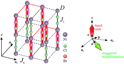
Figure 1: Left: a sketch of DTNX structure with only one tetragonal sublattice of the relevant ions shown. The principal Hamiltonian (1) is also illustrated: $D$ is the on-site planar anisotropy, solid bonds indicate stronger exchange along the “chains” $J_{c}$ and dashed bonds indicate weaker in-plane exchange $J_{a}$. Near the Br-substituted sites these values are affected. Right: the geometry conventions used in the paper.

There are two inequivalent halogen sites in the structure. In Ni(Cl_1-xBr_x)₂$\cdot$4SC(NH₂)₂ the Br substitute tends to occupy a particular one of them Yu et al. (2012a); Orlova et al. (2017). This distorts the environment of Ni²⁺ and strongly affects the covalency of the Ni-halogen bonds. In turn, interactions are strongly modified, especially $J_{c}$ for which the two-halide bond is the primary superexchange mediator Povarov et al. (2015). Recent NMR Orlova et al. (2017) and theoretical Dupont et al. (2017a); *Dupont_PRB_2017_BrDTNmicro studies suggest that these modification of the Hamiltonian (1) parameters are very local.

II.2 Experimental details

The bulk of the work reported here is inelastic neutron scattering experiments on 99% deuterated single crystal samples of Ni(Cl_1-xBr_x)₂$\cdot$4SC(NH₂)₂. These were grown from aqueous solution using the temperature gradient method as described in Yankova et al. (2012); Wulf (2015). The Br concentration in as-grown crystals was verified by means of single-crystals x-ray diffraction on an APEX-II Bruker diffractometer and determined to be $x=0.21(2)$.

Time-of-flight inelastic neutron measurements were performed on the IN5 spectrometer at Institute Laue–Langevin Ollivier and Mutka (2011). A sample consisting of two co-aligned crystals with total mass of about $0.2$ g was installed onto the cold finger of a ³He-⁴He dilution refrigerator. The scattering plane was $(1,-1,0)$ as defined by its normal. This provided access to the momentum transfers of $\mathbf{Q}=(h,~{}h,~{}l)=h(\mathbf{a}_{1}^{\ast}+\mathbf{a}_{2}^{\ast})+l\mathbf{c}^{\ast}$ type. The measurements were performed at a base temperature of about $70$ mK using neutrons with incident energies $E_{\text{i}}=2.26$ meV. Scattering data were recorded with a position-sensitive detector array for a sequence of 140 frames with $1^{\circ}$ sample rotation steps. All data were analyzed using Horace software Ewings et al. (2016).

III Results and data analysis

III.1 Overview of the excitation spectrum

An overview of the measured excitation spectrum is given in Fig. 2. It shows a false color plot of neutron scattering intensities as a function of momentum and energy transfer. As indicated in the inset, the momentum transfer follows a sequence of high symmetry directions in the $(h,~{}h,~{}l)$ plane. The spectrum is clearly dominated by a single excitation branch, which remains underdamped in the entire zone. Overall, its dispersion is not dissimilar to that previously measured in the parent compound $x=0$ Zapf et al. (2006) and for $x=0.06$ Povarov et al. (2015) (dotted and dashed lines in Fig. 2). The key difference is that in the present compound there is no excitation gap. This is consistent with notably different thermodynamics, as compared to $x<x_{c}$ (“underdoped”) materials Povarov et al. (2017).

Figure 2: False color map of neutron scattering intensity measured in the $x=0.21(2)$ DTNX sample at $T\simeq 70$ mK. The momentum transfer $\mathbf{Q}$ follow a specific trajectory between high symmetry points of the Brillouin zone (inset). The reference dispersion curves for $x=0$ and $x=0.06$ materials Zapf et al. (2006); Povarov et al. (2015) are shown as dotted and dashed lines. The solid line is a dispersion fit to the present data, as described in the text. Hatching marks the region dominated by parasitic quasielastic scattering.

III.2 Theoretical approach

As mentioned, the ordered moment in the present $x=0.21(2)$ material is significantly reduced compared to the classical expectation of $2\mu_{B}$ per Ni²⁺. Under these circumstances, the standard spin wave theory reaches its applicability limit. To quantitatively analyze the data we instead employed the so-called GSWT approach Zhang et al. (2013); Muniz et al. (2014). We follow the particular formulation for a DTN-like Hamiltonian (1) developed by Matsumoto and Koga Matsumoto and Koga (2007). This method utilizes a basis of local states and is similar to “bond operator theory” Sachdev and Bhatt (1990); Matsumoto et al. (2004) used for treating dimerized spin systems. In the quantum paramagnetic phase the GSWT spectrum features two degenerate bosonic modes with dispersion relations identical to those obtained in the random phase approximation (RPA) Lindgård and Schmid (1993). The ordered state is then treated as the quantum mechanical condensate of such excitations. Here there are three new types of quasiparticles: two transverse spin wave modes ($yy$) and ($zz$) (see schematic in Fig. 1), and one amplitude mode ($xx$). The transverse modes are gapless. Their dispersions are related by a translation by the magnetic propagation vector $\mathbf{Q}_{0}=(1/2,~{}1/2,~{}1/2)$: $\hbar\omega_{yy}(\mathbf{Q})=\hbar\omega_{zz}(\mathbf{Q}+\mathbf{Q}_{0})$. The equal-time structure factor (intensity) $\mathcal{S}_{yy}(\mathbf{Q})$ is generally much larger than $\mathcal{S}_{zz}(\mathbf{Q})$, since the latter corresponds to spin fluctuations along the hard axis. The longitudinal mode has a gap, which is proportional to the ordered moment. Its intensity tends to be smaller than that for the $yy$ spin wave. The exact GSWT expressions for the corresponding dispersion relations and structure factors are given in Appendix A.

III.3 Data analysis

Figure 3: Representative constant-$\mathbf{Q}$ cuts of the measured neutron intensity (symbols). The data is truncated below $\hbar\omega=0.1$ and above $\hbar\omega=1.2$ meV, where instrument background dominates. Solid lines are fits to individual cuts, as described in the text.

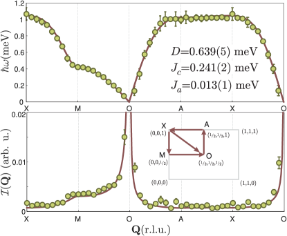
Figure 4: Symbols: dispersion (top) and intensities $\mathcal{I}(\mathbf{Q})=|F(Q)|^{2}P_{yy}(\mathbf{Q})\mathcal{S}_{yy}(\mathbf{Q})$ (bottom) of magnetic excitations determined in fits to individual constant-$\mathbf{Q}$ cuts. In the dispersion plot, the error bars are actually the intrinsic line widths determined from the same fits. The solid line is the GSWT calculation based on Hamiltonian parameters determined in a global fit to the measured dispersion relation.

In order to quantify the dispersion, intrinsic width and intensity of the observed excitations, we analyzed individual constant-$\mathbf{Q}$ cuts of the data for a grid of wave vectors with a step of $\delta Q=0.05$ r.l.u. in both $h$ and $l$ directions. At each wave vector the fitting function was a Voigt profile. Its Gaussian component was the calculated energy-dependent energy resolution of the spectrometer Lowde (1960); *Lechner_1985_TOFresolution. The Lorentzian component represented the intrinsic excitation width and was one of the fit parameters. Also fitted was the peak position, an intensity prefactor and a a flat background. Representative examples of such fits for a few representative points are given in Fig. 3. For high-symmetry reciprocal space directions the fitted peak positions and intensities are plotted against wave vector transfer in Fig. 4.

To obtain the Hamiltonian parameters the dispersion relation determined on the entire wave vector grid was fit using the GSWT result. We attribute the observed scattering to the $yy$ excitation branch. The best fit is obtained with $D=0.639(5)$ meV, $J_{c}=0.241(2)$ meV, and $J_{a}=0.013(1)$ meV. The dispersion relation along high symmetry directions calculated with these values is plotted in a solid line in Fig. 4 (top panel) to illustrate the excellent level of agreement.

A GSWT calculation with these parameters can reproduce the measured intensities as well. This defines the neutron polarization factor, as neutrons are only scattered by magnetization components that are transverse to the momentum transfer. Since a macroscopic sample is bound to split into domains with different orientations of the ordered moment in the tetragonal plane, this effect needs to be averaged accordingly. In our analysis we thus multiplied the mode intensities calculated with GSWT by the polarization factor $P_{yy}(\mathbf{Q})=1-\left(2\pi ha/Q\right)^{2}$. An additional correction was the Ni²⁺ magnetic form factor $|F(Q)|^{2}$ that we included in our calculation within the dipole approximation Prince (2004). With just one additional fit parameter, namely a single overall scale factor, the GSWT model with exchange and anisotropy constants as obtained in dispersion fit gives an excellent agreement with the measurement (solid line in the bottom panel of Fig. 4).

Our data analysis also yields the intrinsic linewidth $\Gamma(\mathbf{Q})$ of excitations as a function of wave vector. For a direct comparison with previous studies, we choose to plot the energy dependence of the linewidth $\Gamma(\omega)$, averaged over the Brillouin zone. For our present sample this quantity is shown in Fig. 5 in filled circles. Previously published data for the “underdoped” $x=0.06$ material are plotted in open squares. For reference, the energy resolution of the spectrometer (the same in both studies) is plotted in a dashed line.

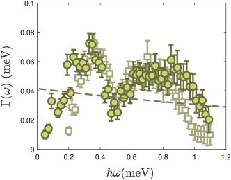
Figure 5: Measured distribution of the intrinsic linewidth as the function of excitation energy. Filled circles are the present data for $x=0.21$ DTNX. Open squares are for $x=0.06$ Povarov et al. (2015). The dashed line is the calculated spectrometer resolution in both cases.

IV Discussion

IV.1 Other GSWT modes

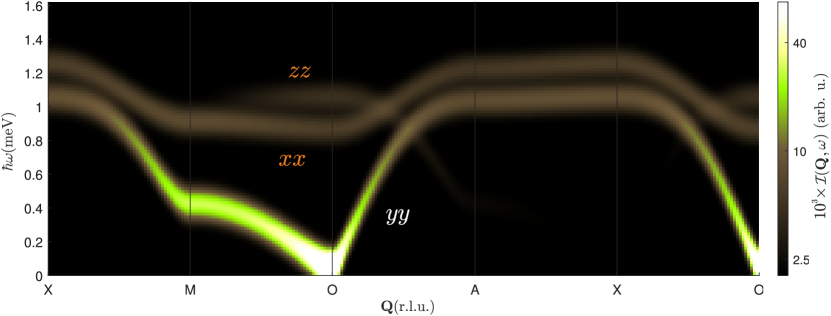
Figure 6: Simulated GSWT spectrum with the background $\mathcal{B}(\mathbf{Q})=2\cdot 10^{-3}$, convoluted with $\sigma=50$ $\mu$eV Gaussian. Polarization factors and magnetic ion form factor are also taken into account.

The agreement of the GSWT predictions for the $yy$ mode with experiment is remarkable, but what about the other two excitation branches? In Fig. 6 we show the GSWT calculation for all three polarizations, based on the Hamiltonian parameters obtained in the fit above. The polarization factors for each mode and the magnetic form factor are accounted for as appropriate. All modes in this simulation have zero intrinsic line widths, as appropriate for GSWT. This simulation tells us that the out of plane transverse $zz$ mode could well be too weak to be observable in the present experiment. However, the longitudinal $xx$ mode would be strong enough to be seen, if only it were underdamped. It is well understood however that a sharp longitudinal excitation is an artifact of GSWT. In fact, longitudinal modes in antiferromagnets with gapless spin waves are known to be prone to decays into transverse modes Podolsky et al. (2011); Zhitomirsky and Chernyshev (2013). Being overdamped, they cannot be even associated with a peak feature in the spectrum. In the few materials Merchant et al. (2008); Hong et al. (2017); Jain et al. (2017) where longitudinal modes are observed, they are stabilized by Ising-like anisotropy effects absent in DTNX. We conclude that detecting only one of the excitation branches predicted by GSWT is actually not that surprising.

IV.2 Hamiltonian parameters

Hamiltonian (1)		clean		“underdoped”		“overdoped”
parameters		$x=0$		$x=0.06$		$x=0.21(2)$
(meV)		Ref.  Zapf et al. (2006)		Ref. Povarov et al. (2015)		present work
$D$		0.780(3)		0.792(3)		0.639(5)
$J_{c}$		0.141(3)		0.155(1)		0.241(2)
$J_{a}$		0.014(1)		0.0158(3)		0.013(1)

Table 1: Parameters of Hamiltonian (1) for various members of DTNX family experimentally determined by means of GSWT analysis of inelastic neutron scattering data.

As already mentioned, in the quantum paramagnetic phase GSWT is equivalent to the RPA. This allows a meaningful comparison of the Hamiltonian parameters that we obtain for the “overdoped” $x=0.21(2)>x_{c}$ material to those previously determined for the parent compound  Zapf et al. (2006) and for the “underdoped” $x=0.06$ system Povarov et al. (2015).

This comparison is made in Table 1. The left panel of Fig. 7 positions the three compounds on the phase diagram calculated with the Mean Field (MF) or GSWT approximations. The MF boundary between the gapped and ordered phases, i.e., the line of gap closure, corresponds to $D=4J_{c}+8J_{a}$. In this context, the $x=0.21(2)$ material lands deep inside the ordered phase. The complication is that the RPA and GSWT exchange constants are known to be strongly renormalized compared to actual values. For the gapped compounds this renormalization can be accounted for by the self-consistent “Lagrange multiplier method” Sachdev and Bhatt (1990); Zhang et al. (2013). The phase space of actual, rather than renormalized, Hamiltonian parameters is shown in the right panel of Fig 7. This plot also shows the numerically computed phase boundaries for weakly-coupled $S=1$ spin chains with planar anisotropy  Sakai and Takahashi (1990); Wierschem and Sengupta (2014a); *WierschemSengupta_PRL_2014_DTNlikeGS. Unfortunately, this procedure cannot be applied to determine the actual Hamiltonian parameters in our “overdoped” system, which is already in the ordered phase Zhang et al. (2013).

IV.3 Disorder

Ni(Cl_1-xBr_x)₂$\cdot$4SC(NH₂)₂ obviously contains a large amount of structural disorder which, as mentioned above, translates into a randomness of local Hamiltonian parameters. While one could expect this randomness to be stronger in our $x=0.21(2)$ material than in the previously studied $x=0.06$ system, the comparison of intrinsic line widths (Fig. 5) show that the two are comparable. Moreover, despite rather distinct ground states, the line width distributions are very similar, with maxima around $0.3$ and $0.8$ meV, and a starpening of magnon peaks at the top and bottom of the spectrum. We conclude that across the concentration range the magnon instability due to randomness must be governed by a single mechanism.

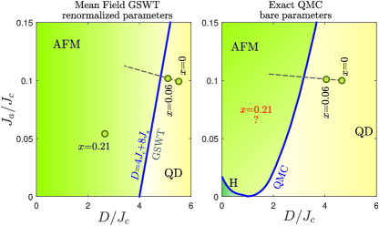
Figure 7: Ground state phase diagrams of Hamiltonian (1). Left panel: Phase diagram in the mean field approximation including quantum disordered (QD) and antiferromagnetically ordered (AF) phases Matsumoto and Koga (2007). The points, locating three different DTNX family members on this phase diagram are obtained from GSWT without taking the quantum corrections into account. Right panel: the exact phase diagram, obtained by Quantum Monte–Carlo (QMC) calculations. A new Haldane phase (H) appears in the decoupled Heisenberg chain limit. The experimental points for $x=0$ and $x=0.06$ materials of DTNX family now correspond to the estimated bare microscopic parameters Zapf et al. (2006); Povarov et al. (2015). Dashed line shows the linear low bromine concentration trend in both figures.

V Summary

The three take-home messages of this study are: 1) Transverse spin excitations in the entire series of DTNX materials, both “underdoped” and “overdoped”, are remarkably well described by GSWT. 2) The underdamped longitudinal mode, a known artefact of GSWT, is absent in the DTNX. 3) The effect of chemical disorder is rather subtle and for the most part amounts to a moderate broadening of magnons.

Appendix A GSWT exact results

In this Appendix we recite the GSWT theoretical results for the DTN-like material obtained by Matsumoto and Koga Matsumoto and Koga (2007). We would like to start with the excitations in the ordered phase. First, the following auxiliary notation are introduced:

$$u,v=\sqrt{\frac{1}{2}\left(1\pm\frac{D}{4J_{c}+8J_{a}}\right)},$$ (2)

$$\gamma(\mathbf{Q})=2J_{c}\cos(\mathbf{Q\cdot c})+2J_{a}\left[\cos(\mathbf{Q\cdot a_{1}})+\cos(\mathbf{Q\cdot a_{2}})\right].$$ (3)

Note, that within GSWT $2\gamma(0)=4J_{c}+8J_{a}$ corresponds to the critical value of single-ion anisotropy $D_{c}$ at which the antiferromagnetic order is suppressed.

Then, Eqs. (2) and (3) are plugged into the following four terms related to longitudinal ($L$) and transverse ($T$) excitation channels:

$$\epsilon_{L}(\mathbf{Q}) = (u^{2}-v^{2})D+4u^{2}v^{2}(4J_{c}+8J_{a})$$

$$+(u^{2}-v^{2})^{2}\gamma(\mathbf{Q}),$$

$$\delta_{L}(\mathbf{Q}) = (u^{2}-v^{2})^{2}\gamma(\mathbf{Q}),$$ (4)

$$\epsilon_{T}(\mathbf{Q}) = u^{2}D+2u^{2}v^{2}(4J_{c}+8J_{a})+(u^{2}-v^{2})\gamma(\mathbf{Q}),$$

$$\delta_{T}(\mathbf{Q}) = \gamma(\mathbf{Q}).$$

Finally, the terms (A) are used to construct the dispersion relations and the corresponding equal-time structure factors (intensities) of the spin wave excitations:

$$\hbar\omega_{xx}(\mathbf{Q})=\sqrt{\epsilon_{L}(\mathbf{Q})^{2}-\delta_{L}(\mathbf{Q})^{2}},$$ (5)

$$\hbar\omega_{yy}(\mathbf{Q})=\sqrt{\epsilon_{T}(\mathbf{Q})^{2}-\delta_{T}(\mathbf{Q})^{2}},$$ (6)

$$\hbar\omega_{zz}(\mathbf{Q})=\sqrt{\epsilon_{T}(\mathbf{Q}+\mathbf{Q}_{0})^{2}-\delta_{T}(\mathbf{Q}+\mathbf{Q}_{0})^{2}},$$ (7)

$$\mathcal{S}_{xx}(\mathbf{Q})=A(u^{2}-v^{2})^{2}\sqrt{\frac{\epsilon_{L}(\mathbf{Q})-\delta_{L}(\mathbf{Q})}{\epsilon_{L}(\mathbf{Q})+\delta_{L}(\mathbf{Q})}},$$ (8)

$$\mathcal{S}_{yy}(\mathbf{Q})=Au^{2}\sqrt{\frac{\epsilon_{T}(\mathbf{Q})-\delta_{T}(\mathbf{Q})}{\epsilon_{T}(\mathbf{Q})+\delta_{T}(\mathbf{Q})}},$$ (9)

$$\mathcal{S}_{zz}(\mathbf{Q})=Av^{2}\sqrt{\frac{\epsilon_{T}(\mathbf{Q+Q_{0}})+\delta_{T}(\mathbf{Q+Q_{0}})}{\epsilon_{T}(\mathbf{Q+Q_{0}})-\delta_{T}(\mathbf{Q+Q_{0}})}}.$$ (10)

In the equations above $A$ is the overall normalization parameter, used for direct comparison with the experimental neutron scattering intensities.

In case of quantum paramagnetic phase the $zz$ excitation vanishes, while $xx$ and $yy$ excitations converge to a single doubly degenerate mode. Its dispersion is simply:

$$\hbar\omega_{PM}(\mathbf{Q})=\sqrt{D^{2}+2D\gamma(\mathbf{Q})}.$$ (11)

The corresponding intensity is given by:

$$\mathcal{S}_{PM}(\mathbf{Q})=A\frac{D}{\hbar\omega_{PM}(\mathbf{Q})},$$ (12)

with $A$ being the same as in Eqs. (8) – (10).

References

- Sachdev (2008) S. Sachdev, “Quantum magnetism and criticality,” Nat. Physics 4, 173 (2008).
- Oosawa et al. (2003) A. Oosawa, M. Fujisawa, T. Osakabe, K. Kakurai, and H. Tanaka, “Neutron Diffraction Study of the Pressure-Induced Magnetic Ordering in the Spin Gap System TlCuCl3,” J. Phys. Soc. Jpn. 72, 1026–1029 (2003).
- Rüegg et al. (2008) Ch. Rüegg, B. Normand, M. Matsumoto, A. Furrer, D. F. McMorrow, K. W. Krämer, H. U. Güdel, S. N. Gvasaliya, H. Mutka, and M. Boehm, “Quantum Magnets under Pressure: Controlling Elementary Excitations in ,” Phys. Rev. Lett. 100, 205701 (2008).
- Merchant et al. (2008) P. Merchant, B. Normand, K. W. Krämer, M. Boehm, D. F. McMorrow, and Ch. Rüegg, “Quantum and classical criticality in a dimerized quantum antiferromagnet,” Nat. Physics 10, 373 (2008).
- Thede et al. (2014) M. Thede, A. Mannig, M. Månsson, D. Hüvonen, R. Khasanov, E. Morenzoni, and A. Zheludev, “Pressure-induced quantum critical and multicritical points in a frustrated spin liquid,” Phys. Rev. Lett. 112, 087204 (2014).
- Perren et al. (2015) G. Perren, J. S. Möller, D. Hüvonen, A. A. Podlesnyak, and A. Zheludev, “Spin dynamics in pressure-induced magnetically ordered phases in ,” Phys. Rev. B 92, 054413 (2015).
- Mannig et al. (2016) A. Mannig, J. S. Möller, M. Thede, D. Hüvonen, T. Lancaster, F. Xiao, R. C. Williams, Z. Guguchia, R. Khasanov, E. Morenzoni, and A. Zheludev, “Effect of disorder on a pressure-induced magnetic quantum phase transition,” Phys. Rev. B 94, 144418 (2016).
- Kurita and Tanaka (2016) N. Kurita and H. Tanaka, “Magnetic-field- and pressure-induced quantum phase transition in proved via magnetization measurements,” Phys. Rev. B 94, 104409 (2016).
- Hayashida et al. (2018) S. Hayashida, O. Zaharko, N. Kurita, H. Tanaka, M. Hagihala, M. Soda, S. Itoh, Yo. Uwatoko, and T. Masuda, “Pressure-induced quantum phase transition in the quantum antiferromagnet ,” Phys. Rev. B 97, 140405 (2018).
- Giamarchi et al. (2008) T. Giamarchi, C. Rüegg, and O. Tchernyshyov, “Bose-Einstein condensation in magnetic insulators,” Nat. Physics 4, 198 (2008).
- Zapf et al. (2014) V. Zapf, M. Jaime, and C. D. Batista, “Bose-Einstein condensation in quantum magnets,” Rev. Mod. Phys. 86, 563 (2014).
- Nikuni et al. (2000) T. Nikuni, M. Oshikawa, A. Oosawa, and H. Tanaka, “Bose-Einstein Condensation of Dilute Magnons in ,” Phys. Rev. Lett. 84, 5868–5871 (2000).
- Toda et al. (2005) M. Toda, Y. Fujii, S. Kawano, T. Goto, M. Chiba, S. Ueda, K. Nakajima, K. Kakurai, J. Klenke, R. Feyerherm, M. Meschke, H. A. Graf, and M. Steiner, “Field-induced magnetic order in the singlet-ground-state magnet ,” Phys. Rev. B 71, 224426 (2005).
- Stone et al. (2007) M. B. Stone, C. Broholm, D. H. Reich, P. Schiffer, O. Tchernyshyov, P. Vorderwisch, and N. Harrison, “Field-driven phase transitions in a quasi-two-dimensional quantum antiferromagnet,” New J. Phys. 9, 31 (2007).
- Yu et al. (2012a) R. Yu, L. Yin, N. S. Sullivan, J. S. Xia, C. Huan, A. Paduan-Filho, N. F. Oliveira Jr, S. Haas, A. Steppke, C. F. Miclea, F. Weickert, R. Movshovich, E.-D. Mun, B. L. Scott, V. S. Zapf, and T. Roscilde, “Bose glass and Mott glass of quasiparticles in a doped quantum magnet,” Nature 489, 379 (2012a).
- Yu et al. (2012b) R. Yu, C. F. Miclea, F. Weickert, R. Movshovich, A. Paduan-Filho, V. S. Zapf, and T. Roscilde, “Quantum critical scaling at a Bose-glass/superfluid transition: Theory and experiment for a model quantum magnet,” Phys. Rev. B 86, 134421 (2012b).
- Wulf et al. (2013) E. Wulf, D. Hüvonen, J.-W. Kim, A. Paduan-Filho, E. Ressouche, S. Gvasaliya, V. Zapf, and A. Zheludev, “Criticality in a disordered quantum antiferromagnet studied by neutron diffraction,” Phys. Rev. B 88, 174418 (2013).
- Povarov et al. (2015) K. Yu. Povarov, E. Wulf, D. Hüvonen, J. Ollivier, A. Paduan-Filho, and A. Zheludev, “Dynamics of a bond-disordered quantum magnet near criticality,” Phys. Rev. B 92, 024429 (2015).
- Povarov et al. (2017) K. Yu. Povarov, A. Mannig, G. Perren, J. S. Möller, E. Wulf, J. Ollivier, and A. Zheludev, “Quantum criticality in a three-dimensional spin system at zero field and pressure,” Phys. Rev. B 96, 140414 (2017).
- Matsumoto and Koga (2007) M. Matsumoto and M. Koga, “Longitudinal spin-wave mode near quantum critical point due to uniaxial anisotropy,” J. Phys. Soc. Jap. 76, 073709 (2007).
- Zhang et al. (2013) Z. Zhang, K. Wierschem, I. Yap, Y. Kato, C. D. Batista, and P. Sengupta, “Phase diagram and magnetic excitations of anisotropic spin-one magnets,” Phys. Rev. B 87, 174405 (2013).
- Muniz et al. (2014) R. A. Muniz, Y. Kato, and C. D. Batista, “Generalized spin-wave theory: Application to the bilinear–biquadratic model,” Progr. Theor. Exp. Phys 2014, 1 (2014).
- Zapf et al. (2006) V. S. Zapf, D. Zocco, B. R. Hansen, M. Jaime, N. Harrison, C. D. Batista, M. Kenzelmann, C. Niedermayer, A. Lacerda, and A. Paduan-Filho, “Bose-Einstein Condensation of Nickel Spin Degrees of Freedom in ,” Phys. Rev. Lett. 96, 077204 (2006).
- Zvyagin et al. (2007) S. A. Zvyagin, J. Wosnitza, C. D. Batista, M. Tsukamoto, N. Kawashima, J. Krzystek, V. S. Zapf, M. Jaime, N. F. Oliveira, and A. Paduan-Filho, “Magnetic Excitations in the Spin-1 Anisotropic Heisenberg Antiferromagnetic Chain System ,” Phys. Rev. Lett. 98, 047205 (2007).
- Yin et al. (2008) L. Yin, J. S. Xia, V. S. Zapf, N. S. Sullivan, and A. Paduan-Filho, “Direct Measurement of the Bose-Einstein Condensation Universality Class in at Ultralow Temperatures,” Phys. Rev. Lett. 101, 187205 (2008).
- Blinder et al. (2017) R. Blinder, M. Dupont, S. Mukhopadhyay, M. S. Grbić, N. Laflorencie, S. Capponi, H. Mayaffre, C. Berthier, Ar. Paduan-Filho, and M. Horvatić, “Nuclear magnetic resonance study of the magnetic-field-induced ordered phase in the compound,” Phys. Rev. B 95, 020404 (2017).
- Wulf et al. (2015) E. Wulf, D. Hüvonen, R. Schönemann, H. Kühne, T. Herrmannsdörfer, I. Glavatskyy, S. Gerischer, K. Kiefer, S. Gvasaliya, and A. Zheludev, “Critical exponents and intrinsic broadening of the field-induced transition in ,” Phys. Rev. B 91, 014406 (2015).
- Orlova et al. (2017) A. Orlova, R. Blinder, E. Kermarrec, M. Dupont, N. Laflorencie, S. Capponi, H. Mayaffre, C. Berthier, A. Paduan-Filho, and M. Horvatić, “Nuclear Magnetic Resonance Reveals Disordered Level-Crossing Physics in the Bose-Glass Regime of the Br-Doped Compound at a High Magnetic Field,” Phys. Rev. Lett. 118, 067203 (2017).
- Dupont et al. (2017a) M. Dupont, S. Capponi, and N. Laflorencie, “Disorder-Induced Revival of the Bose-Einstein Condensation in at High Magnetic Fields,” Phys. Rev. Lett. 118, 067204 (2017a).
- Dupont et al. (2017b) M. Dupont, S. Capponi, M. Horvatić, and N. Laflorencie, “Competing Bose-glass physics with disorder-induced Bose-Einstein condensation in the doped antiferromagnet at high magnetic fields,” Phys. Rev. B 96, 024442 (2017b).
- Yankova et al. (2012) T. Yankova, D. Hüvonen, S. Mühlbauer, D. Schmidiger, E. Wulf, S. Zhao, A. Zheludev, T. Hong, V. O. Garlea, R. Custelcean, and G. Ehlers, “Crystals for neutron scattering studies of quantum magnetism,” Philos. Mag. 92, 2629 (2012).
- Wulf (2015) E. Wulf, Experimental studies on quantum magnets in the presence of disorder (PhD thesis, ETH Zürich, 2015).
- Ollivier and Mutka (2011) J. Ollivier and H. Mutka, “IN5 cold neutron time-of-flight spectrometer, prepared to tackle single crystal spectroscopy,” J. Phys. Soc. Jap. 80, SB003 (2011).
- Ewings et al. (2016) R. A. Ewings, A. Buts, M. D. Le, J. van Duijn, I. Bustinduy, and T. G. Perring, “Horace: Software for the analysis of data from single crystal spectroscopy experiments at time-of-flight neutron instruments,” Nucl. Instrum. Methods Phys. Res., Sect. A 834, 132 (2016).
- Sachdev and Bhatt (1990) S. Sachdev and R. N. Bhatt, “Bond-operator representation of quantum spins: Mean-field theory of frustrated quantum Heisenberg antiferromagnets,” Phys. Rev. B 41, 9323 (1990).
- Matsumoto et al. (2004) M. Matsumoto, B. Normand, T. M. Rice, and M. Sigrist, “Field- and pressure-induced magnetic quantum phase transitions in ,” Phys. Rev. B 69, 054423 (2004).
- Lindgård and Schmid (1993) P.-A. Lindgård and B. Schmid, “Theory of singlet-ground-state magnetism: Application to field-induced transitions in and ,” Phys. Rev. B 48, 13636–13646 (1993).
- Lowde (1960) R. D. Lowde, “The principles of mechanical neutron-velocity selection,” J. Nucl. Energy, Part A: Reactor Science 11, 69 (1960).
- Lechner (1985) R. E. Lechner, Neutron scattering in the nineties (International Atomic Energy Agency, Vienna, 1985).
- Prince (2004) E. Prince, International Tables for Crystallography, Volume C: Mathematical, Physical and Chemical Tables, International Tables for Crystallography (Wiley, U.K., 2004).
- Podolsky et al. (2011) D. Podolsky, A. Auerbach, and D. P. Arovas, “Visibility of the amplitude (Higgs) mode in condensed matter,” Phys. Rev. B 84, 174522 (2011).
- Zhitomirsky and Chernyshev (2013) M. E. Zhitomirsky and A. L. Chernyshev, “Colloquium: Spontaneous magnon decays,” Rev. Mod. Phys. 85, 219–242 (2013).
- Hong et al. (2017) T. Hong, M. Matsumoto, Y. Qiu, W. Chen, T. R. Gentile, S. Watson, F. F. Awwadi, M. M. Turnbull, S. E. Dissanayake, H. Agrawal, R. Toft-Petersen, B. Klemke, K. Coester, K. P. Schmidt, and D. A. Tennant, “Higgs amplitude mode in a two-dimensional quantum antiferromagnet near the quantum critical point,” Nat. Phys. 13, 638 (2017).
- Jain et al. (2017) A. Jain, M. Krautloher, J. Porras, G. H. Ryu, D. P. Chen, D. L. Abernathy, J. T. Park, A. Ivanov, J. Chaloupka, G. Khaliullin, Keimer B., and B. J. Kim, “Higgs mode and its decay in a two-dimensional antiferromagnet,” Nat. Phys. 13, 633 (2017).
- Sakai and Takahashi (1990) T. Sakai and M. Takahashi, “Effect of the Haldane gap on quasi-one-dimensional systems,” Phys. Rev. B 42, 4537 (1990).
- Wierschem and Sengupta (2014a) K. Wierschem and P. Sengupta, “Characterizing the Haldane phase in quasi-one-dimensional spin-1 Heisenberg antiferromagnets,” Mod. Phys. Lett. B 28, 1430017 (2014a).
- Wierschem and Sengupta (2014b) K. Wierschem and P. Sengupta, “Quenching the Haldane Gap in Spin-1 Heisenberg Antiferromagnets,” Phys. Rev. Lett. 112, 247203 (2014b).