*[arabic]figure *[arabic]table disposition [toc]toc.1toc.1ContentsContentstoc.1

Supersymmetric Models in Light of
Improved Higgs Mass Calculations

E. Bagnaschi¹, H. Bahl², J. Ellis³, J. Evans⁴, T. Hahn²,

S. Heinemeyer⁵, W. Hollik², K. A. Olive⁶, S. Paßehr⁷,

H. Rzehak⁸, I. V. Sobolev⁹, G. Weiglein⁹ and J. Zheng^10
1Paul Scherrer Institut, CH-5232 Villigen PSI, Switzerland
²Max-Planck-Institut für Physik, Föhringer Ring 6, D-80805 Munich, Germany
³Theoretical Particle Physics and Cosmology Group, Dept. of Physics, King’s College London,
London WC2R 2LS, UK;
National Institute of Chemical Physics and Biophysics, Rävala 10, 10143 Tallinn, Estonia;
Theory Division, CERN, CH-1211 Geneva 23, Switzerland
⁴School of Physics, KIAS, Seoul 130-722, Korea
⁵Instituto de Física Teórica, Universidad Autónoma de Madrid Cantoblanco, 28049 Madrid, Spain;
Campus of International Excellence UAM+CSIC, Cantoblanco, 28049, Madrid, Spain;
Instituto de Física de Cantabria (CSIC-UC), E-39005 Santander, Spain
⁶William I. Fine Theoretical Physics Institute, School of Physics and Astronomy, Univ. of Minnesota, Minneapolis, MN 55455, USA
⁷Sorbonne Université, CNRS, Laboratoire de Physique Théorique et Hautes Énergies (LPTHE), UMR 7589,
4 Place Jussieu, F–75252 Paris CEDEX 05, France
⁸CP3-Origins, University of Southern Denmark, Odense, Denmark
⁹DESY, Notkestr. 85, D-22607 Hamburg, Germany
¹⁰Department of Physics, University of Tokyo, Bunkyo-ku, Tokyo 113-0033, Japan

Abstract

We discuss the parameter spaces of supersymmetry (SUSY) scenarios taking into account the improved Higgs-mass prediction provided by FeynHiggs 2.14.1. Among other improvements, this prediction incorporates three-loop renormalization-group effects and two-loop threshold corrections, and can accommodate three separate mass scales: $m_{\tilde{q}}$ (for squarks), $m_{\tilde{g\,}\!}$ (for gluinos) and $m_{\tilde{\chi}}$ (for electroweakinos). Furthermore, it contains an improved treatment of the $\overline{\mathrm{DR}}$ scalar top parameters avoiding problems with the conversion to on-shell parameters, that yields more accurate results for large SUSY-breaking scales. We first consider the CMSSM, in which the soft SUSY-breaking parameters $m_{0}$ and $m_{1/2}$ are universal at the GUT scale, and then sub-GUT models in which universality is imposed at some lower scale. In both cases, we consider the constraints from the Higgs-boson mass $M_{h}$ in the bulk of the $(m_{0},m_{1/2})$ plane and also along stop coannihilation strips where sparticle masses may extend into the multi-TeV range. We then consider the minimal anomaly-mediated SUSY-breaking (mAMSB) scenario, in which large sparticle masses are generic. In all these scenarios the substantial improvements between the calculations of $M_{h}$ in FeynHiggs 2.14.1 and FeynHiggs 2.10.0, which was used in an earlier study, change significantly the preferred portions of the models’ parameter spaces. Finally, we consider the pMSSM11, in which sparticle masses may be significantly smaller and we find only small changes in the preferred regions of parameter space.

CERN-TH/2018-185, DESY-18-182, PSI-PR-18-11, UMN–TH–3801/18,
FTPI–MINN–18/18, IFT–UAM/CSIC–18-081, KIAS-P18095,
KCL-PH-TH/2018-41, MPP-2018-239, CP3-Origins-2018-039 DNRF90

1 Introduction

Given the persistent absence of any signal in the searches for supersymmetric particles at the Large Hadron Collider (LHC) and in direct searches for supersymmetric dark matter (DM), there is strengthened emphasis on the information about the scale of supersymmetry (SUSY) that can be obtained indirectly from other measurements. The Higgs-boson discovery [1, 2] at the LHC opened a new window with the SUSY Higgs-boson mass as a precision observable. The Minimal Supersymmetric Standard Model (MSSM) [3, 4] contains—in contrast to the single Higgs doublet of the Standard Model (SM)—two Higgs doublets. In the ${\cal CP}$-conserving case this leads to a physical spectrum consisting of two ${\cal CP}$-even neutral Higgs bosons, $h$ and $H$, one ${\cal CP}$-odd, $A$, and two charged Higgs bosons, $H^{\pm}$. At the tree level the Higgs sector can be described, besides the SM parameters, by two additional input parameters, conveniently chosen to be the mass of the ${\cal CP}$-odd Higgs boson, $M_{A}$, (or the mass of the charged Higgs, $M_{H^{\pm}}$) and the ratio of the two vacuum expectation values, $\tan\beta\equiv v_{2}/v_{1}$. The light (or heavy) neutral ${\cal CP}$-even MSSM Higgs boson can be interpreted as the signal discovered at $\mathord{\sim}\,125~{}\mathrm{GeV}$ [5].

Prominent among the predicted quantities is the mass of the light ${\cal CP}$-even Higgs boson, $M_{h}$, which can be calculated in terms of the SM parameters and the soft SUSY-breaking parameters. As is well known, tree-level calculations implied that $M_{h}<M_{Z}$ in the MSSM, whereas one-loop calculations raised the possibility that $M_{h}>M_{Z}$ [6, 7, 8]. The more complete multi-loop calculations of $M_{h}$ that have become available subsequently (as summarized in Section 2) can accommodate comfortably the measured value $M_{h}\simeq 125$ GeV [9], and the similarities of the measured Higgs couplings to those in the SM [10] are also consistent with the MSSM.

The question then arises whether these successes of the MSSM can be used to estimate reliably the masses of SUSY particles such as the scalar top quarks (stops), with the corollary question what ranges of their masses are compatible with the strengthening lower limits from the LHC on sparticle masses. Several of us studied these questions in the context of data from LHC Run 1, using the FeynHiggs 2.10.0 code [11]. A particular emphasis in that analysis was to understand the impact of the combination of fixed-order calculations of $M_{h}$ and results obtained in an Effective Field Theory (EFT) approach, which had recently been accomplished at that time and allowed the resummation of large logarithmic contributions, stabilizing the calculation of $M_{h}$ for large stop mass scales [12].

During LHC Run 2 the ATLAS and CMS experiments have been pushing the lower limits on the masses of some strongly-interacting sparticles into the $1$–$2$ TeV range. It is therefore of key importance to have available calculations of the Higgs mass that are as accurate as possible when one or more soft SUSY-breaking parameters are in the multi-TeV range, and there may be a rather large hierarchy between different supersymmetric mass scales.

Important steps in this direction have been taken since the release of FeynHiggs 2.10.0. Many of these advances in the prediction of $M_{h}$ that are particularly important for sparticle masses in the multi-TeV range are incorporated in the recent release of FeynHiggs 2.14.1. These include three-loop renormalization-group equations (RGEs) with electroweak effects, as well as corresponding two-loop threshold corrections including the possibility of non-degenerate stop mass parameters. Moreover, whereas only a single SUSY-breaking scale was incorporated in FeynHiggs 2.10.0, three distinct scales can be accommodated in FeynHiggs 2.14.1. These are the squark and gluino masses, $m_{\tilde{q}}$, $m_{\tilde{g\,}\!}$, and a scale $m_{\tilde{\chi}}$ characterizing the overall electroweakino mass scale, thus making the connection to DM, assuming it to be given by the lightest neutralino, $\tilde{\chi}^{0}_{1}$ [13, 14]. In addition, problems that occur when combining an infinite tower of resummed logarithms with a fixed-order result where $\overline{\mathrm{DR}}$ input parameters of the scalar top sector have been converted into the corresponding parameters of the on-shell (OS) renormalization scheme can now be avoided by performing the calculation directly in the $\overline{\mathrm{DR}}$ scheme. Finally a new, improved procedure for determining the poles of the Higgs-boson propagator matrix has been introduced. Section 2.1 contains a review of FeynHiggs 2.14.1 and its relations to other codes for calculating $M_{h}$ in the MSSM, and Section 2.2 makes a specific comparison of FeynHiggs 2.14.1 with FeynHiggs 2.10.0.

In Section 3 of this paper we explore the significance of these advances for a number of MSSM scenarios with different phenomenological features that are sensitive to different aspects of FeynHiggs 2.14.1. The first of these is the CMSSM [16, 17, 18, 19, 20], in which the soft SUSY-breaking scalar mass parameter $m_{0}$ and gaugino mass parameter $m_{1/2}$ are each assumed to be universal at the GUT scale $M_{\mathrm{G}UT}$.

The second example is provided by ‘sub-GUT’ models in which this universality is imposed at some scale $M_{\mathrm{i}n}\leq M_{\mathrm{G}UT}$ [21, 17, 18, 20, 22]. The LHC searches impose severe constraints on these models, favoring parameter sets along the stop coannihilation [23, 24, 25, 26, 27] and focus-point strips [28]. These extend out to multi-TeV sparticle masses with stop masses $m_{\tilde{t}_{1,2}}$ that are strongly non-degenerate in general. Moreover, in the focus-point case $m_{\tilde{\chi}^{0}_{1}}\ll m_{\tilde{t}_{1}}$, whereas these masses are very similar along the stop coannihilation strip.

Thirdly, we consider the minimal anomaly-mediated SUSY-breaking (mAMSB) model [29, 30], in which sfermion masses are typically several tens of TeV, whereas values of $m_{\tilde{\chi}^{0}_{1}}\simeq 1$ TeV or ${\simeq}\,3$ TeV are preferred by the DM density constraint. For a recent global analysis of this model taking into account the constraints from Run 1 of the LHC, see [31].

Finally, we consider a phenomenological MSSM scenario [32, 33] with $11$ free parameters specified at the electroweak scale, as has recently been analyzed including LHC Run 2 data in [34]. A priori, this scenario would allow many possible mass hierarchies, as well as many near-degeneracies between sparticle masses that could dilute the classic missing-transverse-energy ($/E_{T}$) signatures at the LHC and permit lighter sparticles than are allowed in the CMSSM and sub-GUT models.

In each of these scenarios, our primary concern is the implications of improvements in the FeynHiggs 2.14.1 calculation of $M_{h}$ (compared to previous, less sophisticated calculations) for the model parameter space.

2 Higgs Mass Calculations

The experimental accuracy of the measured mass of the observed Higgs boson has already reached the level of a precision observable, with an uncertainty of less than $300~{}\mathrm{MeV}$ [9]. This precision should ideally be matched by the theoretical uncertainty in the prediction of the SM-like Higgs-boson mass. In the following we briefly review the status of Higgs-boson mass calculations in the MSSM. Particularly we focus on the implementation in the code FeynHiggs, where we summarize the relevant progress over the last years, emphasizing the differences w.r.t. FeynHiggs 2.10.0, which was used in Ref. [11].

2.1 Status of MSSM Higgs Mass Calculations

The tree-level predictions for the Higgs-boson masses in the MSSM receive large higher-order corrections, which in the case of $M_{h}$ can be of ${\cal O}(100\%)$, see Refs. [35, 36, 37, 38] for reviews. Beyond the one-loop level, the dominant two-loop corrections of ${\cal O}(\alpha_{t}\alpha_{s})$ [39, 40, 41, 42, 43, 44] and ${\cal O}(\alpha_{t}^{2})$ [45, 46] as well as the corresponding corrections of ${\cal O}(\alpha_{b}\alpha_{s})$ [47, 48] and ${\cal O}(\alpha_{t}\alpha_{b})$ [49] have been known for more than a decade (see also Ref. [50, 51, 52, 53] for the ${\cal CP}$-violating case—the last reference going beyond the large-$\tan\beta$ limit employed by Ref. [49]). The $\tan\beta$-enhanced threshold corrections to the bottom Yukawa coupling in the MSSM [54, 55, 56, 57] are included in the resummation of leading contributions from the bottom/scalar bottom sector [47, 49, 48] (see also [58, 59] for corresponding next-to-leading order (NLO) threshold contributions). Momentum-dependent two-loop contributions have also been computed [61, 60, 62, 63, 64].

In the case of SUSY spectra with large mass hierarchies, the fixed-order calculation of the Higgs-boson mass loses its predictive power, due to the appearance of large logarithms of the ratio of the mass scales appearing in the result. To obtain an accurate prediction, the resummation of these logarithms is required. To achieve this goal, the calculation of the Higgs mass has to be cast into the language of Effective Field Theories (EFTs). In this approach, the heavy degrees of freedom are integrated out at their characteristic scale, $M_{S}$, where they enter the matching conditions for the couplings of the low-energy EFT. The RGEs are then used to relate the values of the couplings at $M_{S}$ with those at the low scale, which in the simplest cases is the electroweak scale, where physical observables such as the Higgs mass are computed. In this way, the logarithms of the ratio of the relevant mass scales are taken into account to all orders, while, at the same time, power-suppressed terms of ${\cal O}(v^{2}/M_{S}^{2})$ are neglected, unless higher-dimensional effective operators are matched and included in the low-energy EFT.

The EFT approach was originally developed about $25$ years ago [65, 66, 67]. It has subsequently been used to compute the coefficients of the logarithmic terms appearing in the computation of the Higgs mass at one [68], two [69, 70, 71, 72] and three [73, 74] loops. However, due to the missing ${v^{2}/M_{S}^{2}}$ terms mentioned above, this approach was not competitive with a traditional fixed-order computation in the case of relatively light SUSY scenarios.

The situation has changed in the past few years, due to the renewed interest in scenarios with heavy sparticles caused by the (so far) negative outcomes of the direct searches at the LHC. Moreover, our knowledge of the matching condition for the Higgs quartic coupling in case of the SM as a low-energy EFT now has been extended to all the contributions controlled by the strong and by the third-generation Yukawa couplings at two loops [75, 76, 77, 78]. The codes MhEFT [75], SUSYHD [77] and HSSUSY [79, 80] implement these computations, with the latter including all the available corrections. The more complicated case of a low-energy EFT containing two Higgs doublets also has been studied in several contexts, and several codes are available for this case: MhEFT [81] and several generators [82, 79] based on FlexibleSUSY [83]. Scenarios with $m_{\tilde{g\,}\!}/{m_{\tilde{q}}}\gg 1$, where $m_{\tilde{g\,}\!}$ denotes the gluino mass and $m_{\tilde{q}}$ the scalar top mass scale, are not yet included in any code: the corrections by $\log(m_{\tilde{g\,}\!}/{m_{\tilde{q}}})$ in this hierarchy can presently not yet be resummed. These logarithms could lead to large effects for $m_{\tilde{g\,}\!}/{m_{\tilde{q}}}\gtrsim 4$, a possibility that we comment on later in our numerical analysis.

In order to provide a reliable prediction for the Higgs-boson masses in both low- and high-scale MSSM scenarios, the resummation of the leading and subleading logarithms can be combined with the fixed-order results in the MSSM in the so-called “hybrid approach”, thereby keeping track of the power-suppressed terms that are neglected in a simple EFT approach in which the low-energy EFT does not include higher-dimensional operators . The hybrid approach was first implemented into the code FeynHiggs [86, 87, 41, 73, 88, 12, 84, 85, 89, 15]. In the first version that adopted this method, FeynHiggs 2.10.0, one light Higgs doublet at the low scale was assumed, and the logarithms originating in the top/scalar top sector were resummed [12]. Further refinements have been presented more recently in Refs. [84, 85] . More recently, the hybrid approach has been extended to support such spectra where a full Two-Higgs-Doublet-Model (2HDM) is required as the low-energy EFT [90]. However the latter are not implemented in the current public release of FeynHiggs and therefore they are not used in the current paper, see the discussion in Sect. 2.2 for more details.

For completeness, we also mention here some further corrections that are available in the literature. The full ${\cal O}(\alpha\alpha_{s})$ corrections, including the complete momentum dependence at the two-loop level, became recently available in Ref. [64]. A (nearly) full two-loop effective potential calculation, including also the leading three-loop corrections up to next-to-leading-logarithm (NLL) level, has also been published [91, 92, 61, 74], but is not publicly available as a computer code. Another leading three-loop calculation of ${\cal O}(\alpha_{t}\alpha_{s}^{2})$, depending on various SUSY mass hierarchies, has been performed in [93, 94], and is included in the code H3m that is now available as a stand-alone code, Himalaya [95]. Another approach to the combination of logarithmic resummation with fixed-order results has been presented in Ref. [96] and included in FlexibleSUSY. Subsequently it was also implemented in the SARAH+SPheno [97] framework. We also note that Ref. [98] has studied the issue of the comparison of the theoretical uncertainties in SoftSUSY vs. HSSUSY. Finally, there is a recent calculation [99] that resums terms of leading order in the top Yukawa coupling and NNLO in the strong coupling $\alpha_{s}$, including the three-loop matching coefficient for the quartic Higgs coupling of the SM to the MSSM between the EFT and the fixed-order expression for the Higgs mass, which is available in an updated version of the Himalaya code [95]. However, a detailed numerical comparison of FeynHiggs 2.14.1 with other codes to calculate $M_{h}$ is beyond the scope of this paper.

2.2 Comparison between FeynHiggs 2.14.1 and FeynHiggs 2.10.0

The main advances in FeynHiggs 2.14.1 in comparison to FeynHiggs 2.10.0 are related to the EFT part of the calculation. The resummation of large logarithmic contributions in FeynHiggs 2.10.0 was restricted to $\mathcal{O}(\alpha_{s},\alpha_{t})$ leading-logarithmic (LL) and NLL contributions. Since then, electroweak LL and NLL contributions as well as $\mathcal{O}(\alpha_{s},\alpha_{t})$ next-to NLL (NNLL) contributions have been included. This means, in particular, that the full SM two-loop RGEs and partial three-loop RGEs are used for evolving the couplings between the electroweak scale and the SUSY scale $M_{\text{SUSY}}$. At the SUSY scale, full one-loop threshold corrections and (non-degenerate) threshold corrections of $\mathcal{O}(\alpha_{s}\alpha_{t},\alpha_{t}^{2})$ are used for the matching of the effective SM to the full MSSM, taken from Ref. [76] and from Refs. [77, 78], respectively. Numerically, the electroweak LL and NLL contributions amount to an upward shift of $M_{h}$ of $\mathord{\sim}\,1~{}\mathrm{GeV}$ for a SUSY scale of a few TeV. The NNLL contributions are numerically relevant only for large stop mixing, shifting $M_{h}$ downwards by $\mathord{\sim}\,1~{}\mathrm{GeV}$ for positive $X_{t}$ and upwards by $\mathord{\sim}\,1~{}\mathrm{GeV}$ for negative $X_{t}$ (where the off-diagonal entry in the stop mass matrix for real parameters is $m_{t}\,X_{t}$).

For consistency with this logarithmic precision, one must choose appropriate matching conditions with physical observables at the electroweak scale. This is relevant, in particular, for the $\overline{\mathrm{MS}}$ top quark mass in the SM. In FeynHiggs 2.10.0, the corrections of $\mathcal{O}(\alpha_{s},\alpha_{t})$ in the mass were used. The inclusion of electroweak LL and NLL resummation as well as NNLL of $\mathcal{O}(\alpha_{s},\alpha_{t})$ implies the need to use instead the NNLO $\overline{\mathrm{MS}}$ top quark mass of the SM, as done in FeynHiggs 2.14.1. This modification not only implies changes for large SUSY scales but also impacts significantly the prediction of $M_{h}$ for low SUSY scales, as the shift in the top quark mass affects the non-logarithmic terms that are relevant in this regime. The combined electroweak one-loop as well as the two-loop corrections amount to a downwards shift of the $\overline{\mathrm{MS}}$ top mass of the SM by $\mathord{\sim}\,3~{}\mathrm{GeV}$. The effect on $M_{h}$ is of similar size.

The EFT calculation in the new FeynHiggs version allows one to take into account three different relevant scales. In addition to the SUSY scale $m_{\tilde{q}}$—which was the only scale in FeynHiggs 2.10.0—an electroweakino scale $m_{\tilde{\chi}}$ and a gluino scale $m_{\tilde{g\,}\!}$ are available. They allow one to investigate scenarios with light electroweakinos and/or gluinos. This corresponds to a tower of up to three EFTs (SM, SM with electroweakinos, SM with gluinos, SM with electroweakinos and gluinos). Besides the limitation that $m_{\tilde{g\,}\!}/m_{\tilde{q}}$ should not be too large (see the discussion above, all scales can be chosen independently from each other, though the gluino threshold has a negligible numerical influence in this case. Also, the electroweakino threshold becomes relevant only for a large hierarchy between the electroweakino scale and the SUSY scale (${m_{\tilde{\chi}}}/M_{\text{SUSY}}\lesssim 1/10$), leading to upward shifts of $M_{h}$ of $\mathord{\sim}\,1~{}\mathrm{GeV}$.

The second main advance is a better handling of $\overline{\mathrm{DR}}$ input parameters. The fixed-order calculation of FeynHiggs by default employs a mixed OS/$\overline{\mathrm{DR}}$ scheme for renormalization, in which the parameters of the stop sector are fixed employing the OS scheme. In FeynHiggs 2.10.0, this was the only available renormalization scheme. Therefore, a one-loop conversion between the $\overline{\mathrm{DR}}$ and the OS scheme was employed in the case of $\overline{\mathrm{DR}}$ input parameters. Whilst, for a fixed-order result, such a conversion leads to shifts that are beyond the calculated order, this is no longer the case if a fixed-order result is supplemented by a resummation of large logarithms. As shown in [85], the parameter conversion in this case induces additional logarithmic higher-order terms that can spoil the resummation. As a solution for this issue, an optional $\overline{\mathrm{DR}}$ renormalization of the stop sector is implemented in FeynHiggs 2.14.1. This renders a conversion of the stop parameters unnecessary. Note, however, that the $\overline{\mathrm{DR}}$ sbottom input parameters are still converted to the OS scheme. In particular for large SUSY scales, employing directly the $\overline{\mathrm{DR}}$ scheme for the stop sector parameters and avoiding the conversion to the OS scheme affects the results significantly: e. g., for SUSY scales of $\mathord{\sim}\,20~{}\mathrm{TeV}$, shifts in $M_{h}$ of $\mathord{\sim}\,10~{}\mathrm{GeV}$ were observed compared to the result based on the parameter conversion with the sign of the shift depending on the size of the stop mixing. Also, for low SUSY scales of $\mathord{\sim}\,1~{}\mathrm{TeV}$, the prediction using the $\overline{\mathrm{DR}}$ scheme of the stop sector parameters differs from that employing the conversion to the OS scheme by a downward shift in $M_{h}$ of $\mathord{\sim}\,1~{}\mathrm{GeV}$ in the case of large stop mixing. For SUSY scales below $1~{}\mathrm{TeV}$, where the impact of higher-order logarithmic contributions is relatively small, the observed shift can be interpreted to a large extent as an indication of the possible size of unknown higher-order corrections.

In addition to these improvements, also the Higgs pole determination has been reworked. It was noted in [85] that there is a cancellation between two-loop contributions from sub-loop renormalization and terms arising through the pole determination. In the fixed-order calculation, these terms are of higher order, which are not controlled. In FeynHiggs 2.10.0, the pole determination was performed numerically employing the $\overline{\mathrm{DR}}$ scheme for the Higgs field renormalization. As a consequence of this procedure, the two-loop contributions from sub-loop renormalization were not included at the same order as the terms arising through the pole determination, resulting in an incomplete cancellation. In FeynHiggs 2.14.1 the pole determination has been adapted in order to ensure a complete cancellation. The numerical impact of this improved pole determination procedure increases with rising $M_{\text{SUSY}}$. For $M_{\text{SUSY}}$ in the multi-TeV range, it amounts to a downward shift of $M_{h}$ of $\mathord{\sim}\,1~{}\mathrm{GeV}$.

Finally, the handling of complex input parameters in FeynHiggs was improved. In the fixed-order calculation, the corrections of $\mathcal{O}(\alpha_{t}^{2})$ with full dependence on the phases of complex parameters were implemented [51, 52, 100, 101] (see also [53]). In addition, an interpolation of the EFT calculation in the case of non-zero phases was introduced. Numerically, this can lead to shifts of $M_{h}$ of up to $3~{}\mathrm{GeV}$. As we do not discuss here the effects of the phases of complex parameters, we do not provide further details that can be found in Ref. [15].

Summing up this discussion, we generally expect the prediction of $M_{h}$ of FeynHiggs 2.14.1 to be lower than that of FeynHiggs 2.10.0. In the case of $\overline{\mathrm{DR}}$ input parameters, the large shifts compared to the previous result that employed a conversion to the OS scheme for the renormalization of the stop sector can, however, outweigh the other effects and lead to an overall upward shift of $M_{h}$.

3 Calculations in Specific MSSM Scenarios

In this Section, we illustrate the implications of the improved prediction for $M_{h}$ implemented in FeynHiggs 2.14.1 in the context of several specific MSSM scenarios. The first of these is the CMSSM [16, 17, 18, 19, 20], in which the soft supersymmetry-breaking scalar masses $m_{0}$, the gaugino masses $m_{1/2}$ and the trilinear parameters are all constrained to be universal at the GUT scale. The second scenario we study is a class of sub-GUT models [21, 17, 18, 20, 22], in which these universality relations hold at some renormalization scale $M_{\mathrm{i}n}<M_{\mathrm{G}UT}$, as occurs, e. g., in mirage-mediation models [102]. We then discuss minimal anomaly-mediated models [29, 30], in which the scalar masses are typically much greater than the gaugino masses. For all of these models, we use SSARD [103] to compute the particle mass spectrum and relic density. We note that the convention for $A$ terms used in SSARD is opposite to that used in FeynHiggs. Finally, we study a phenomenological version of the MSSM [32, 33] with $11$ free parameters in the soft supersymmetry-breaking sector, the pMSSM11, allowing for many possible sparticle mass hierarchies. In all cases we assume that the lightest supersymmetric particle (LSP) is the lightest neutralino $\tilde{\chi}^{0}_{1}$ and provides the full DM density [104].

3.1 The Light Higgs-Boson Mass in the CMSSM

The four-dimensional parameter space of the CMSSM that we consider here includes a common input gaugino mass parameter, $m_{1/2}$, a common input soft SUSY-breaking scalar mass parameter, $m_{0}$, and a common trilinear soft SUSY-breaking parameter, $A_{0}$, which are each assumed to be universal at the scale $M_{\mathrm{G}UT}$ (defined as the renormalization scale where the two electroweak gauge couplings are equal), and the ratio of MSSM Higgs vevs, $\tan\beta$. There is also a discrete ambiguity in the sign of the Higgs mixing parameter, $\mu$. In the CMSSM, renormalization group (RG) effects typically produce hierarchies of physical sparticle masses, e. g., between gluinos and electroweakly-interacting gauginos and between squarks and sleptons. The limits from LHC searches for sparticles generally require at least the strongly-interacting sparticles to be relatively heavy. Accurate calculations of $M_{h}$ for MSSM spectra in the multi-TeV range require many of the improvements made in FeynHiggs 2.14.1 compared to FeynHiggs 2.10.0.

Reconciling the cosmological dark matter density [104] of the LSP with the relatively heavy spectra that LHC searches impose on the CMSSM typically requires specific relations between some of the sparticle masses. One such example is the stop coannihilation strip, and another is the focus-point region, which we discuss in the two following subsections.

3.1.1 Stop Coannihilation Strips in the CMSSM

We first consider in some detail examples of stop coannihilation strips. In this case the lighter stop mass $m_{\tilde{t}_{1}}$ and the mass of the LSP, $m_{\tilde{\chi}^{0}_{1}}$, must be quite degenerate. The relic density constraint alone would allow them to weigh several TeV but the allowed range of mass scales is in general restricted by the measurement of $M_{h}$, for more details see Ref. [20] (where FeynHiggs 2.13.1 was used). It is therefore very important that the MSSM calculation of $M_{h}$ along the stop coannihilation strip is optimized.

In Fig. 1 we show four examples of $(m_{1/2},m_{0})$ planes in the CMSSM for $\tan\beta=5$. The upper panels are for $A_{0}=3\,m_{0}$, and the lower panels are for $A_{0}=-4.2\,m_{0}$, assuming that the Higgs mixing parameter $\mu>0$ (left panels) or $\mu<0$ (right panels). In each panel, the brick-red shaded regions are excluded because they feature a charged LSP, which is the ${\tilde{\tau}_{1}}$ in the lower right regions and the ${\tilde{t}_{1}}$ in the upper left regions. There are very narrow dark blue strips close to these excluded regions where the LSP contribution to the dark matter density $\Omega_{\chi}\,h^{2}<0.2$. This range is chosen for clarity, as the range $\Omega_{\mathrm{C}DM}\,h^{2}=0.1193\pm 0.0014$ allowed by cosmology [104] would correspond to a much thinner strip that would be completely invisible. Even with the extended range for the relic density, the line is barely visible. As we discuss in more detail below, the coannihilation strips generally have endpoints at very high masses, where the cross section becomes too small to ensure the proper relic density, even when $m_{\chi}=m_{\tilde{t}_{1}}$. The locations of these endpoints for the Planck range of $\Omega_{\mathrm{C}DM}\,h^{2}$ are indicated by X marks along the strips. The panels feature contours of $M_{h}$ calculated using FeynHiggs 2.14.1 (red solid lines) and FeynHiggs 2.10.0 (thin gray dashed lines). The latter are truncated in regions of large stop masses for $\tan\beta=5$, $A_{0}=3\,m_{0}$ and $\mu>0$, where FeynHiggs 2.10.0 fails to return valid calculations of $M_{h}$.

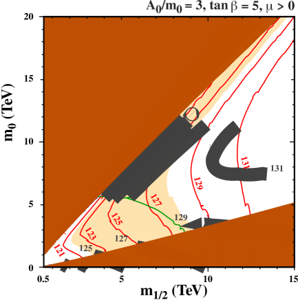
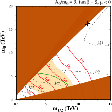
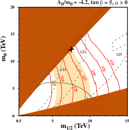
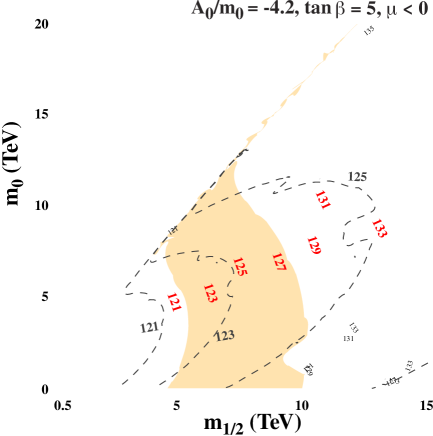
Figure 1: The $(m_{1/2},m_{0})$ planes in the CMSSM for $\tan\beta=5$, $A_{0}=3\,m_{0}$ and $\mu>0$ (upper left panel) or $\mu<0$ (upper right panel), $\tan\beta=5$, $A_{0}=-4.2\,m_{0}$ and $\mu>0$ (lower left panel), and $\tan\beta=5$, $A_{0}=-4.2\,m_{0}$ and $\mu<0$ (lower right panel). The brick-red shaded regions are excluded because they feature a charged LSP, and the panels contain narrow dark blue strips close to these excluded regions where $\Omega_{\chi}\,h^{2}<0.2$, as well as contours of $M_{h}$ calculated using FeynHiggs 2.14.1 (red solid lines) and FeynHiggs 2.10.0 (thin gray dashed lines). The light orange shaded region corresponds to $M_{h}\in[122,128]~{}\mathrm{GeV}$ using FeynHiggs 2.14.1. The X marks the position of the stop coannihilation endpoint. The solid green lines show the lower limit on the proton lifetime calculated in a minimal supersymmetric SU(5) GUT.

Across the $(m_{1/2},m_{0})$ planes we see very different behaviors of the values of the Higgs mass calculated with FeynHiggs 2.14.1 and FeynHiggs 2.10.0, particularly along the stop coannihilation strip, where $m_{\tilde{t}_{1}}$ and $m_{\tilde{\chi}^{0}_{1}}$ may reach several TeV. In such a case, the values of $M_{h}$ given by FeynHiggs 2.14.1 are much more reliable than those obtained with FeynHiggs 2.10.0. In the absence of a detailed uncertainty estimate that depends on the considered region of the parameter space (the update of the uncertainty estimate of FeynHiggs taking into account the latest improvements in the Higgs-mass prediction is still a work in progress), here and later we consider values of the input mass parameters as acceptable for which FeynHiggs 2.14.1 yields $M_{h}=125\pm 3~{}\mathrm{GeV}$, i. e., $M_{h}\in[122,128]~{}\mathrm{GeV}$ (where the additional experimental uncertainty is negligible in comparison). This range from FeynHiggs 2.14.1 is shaded light orange. We discuss this constraint in more detail below, but it is already clear from Fig. 1 that FeynHiggs 2.14.1 favors ranges of $m_{\tilde{t}_{1}}$ and $m_{\tilde{\chi}^{0}_{1}}$ that are quite different from those that would have been indicated by FeynHiggs 2.10.0.

For $A_{0}=3\,m_{0}$ and $\mu>0$, the Higgs mass decreases rapidly as the stop LSP boundary is approached. In this case, the Higgs mass calculated using FeynHiggs 2.10.0 is too small all along the coannihilation strip. Furthermore, we see that FeynHiggs 2.10.0 was not able to produce a reliable result beyond $m_{0}\gtrsim 13$ TeV. Since the endpoint of the coannihilation strip is at much larger $m_{0}$, FeynHiggs 2.14.1 offers a significant improvement. This version of FeynHiggs yields values of the Higgs mass that are significantly larger along the strip, rising as high as $M_{h}=128$ GeV at the endpoint which is not seen in this panel as it lies beyond the shown range in $(m_{1/2},m_{0})$. For $A_{0}=3\,m_{0}$ and $\mu<0$, the Higgs mass is reduced in the newer version of FeynHiggs for most of the strip, though it is larger for $m_{1/2}\gtrsim 6$ TeV. While both versions of FeynHiggs provide strip segments with an acceptable Higgs mass, the location of the segment shifts upwards in the new version. In this case, the Higgs mass is $M_{h}=135$ GeV at the endpoint of the coannihilation strip, so the Higgs mass itself provides a constraint $m_{1/2}\lesssim 6$ TeV, as seen more clearly in the profile plots discussed below. The endpoint is marked by an X at $(m_{1/2},m_{0})\sim(11.3,16.1)~{}\mathrm{TeV}$. When $A_{0}=-4.2\,m_{0}$ and $\mu>0$, we clearly see a large difference between FeynHiggs 2.10.0 and FeynHiggs 2.14.1. In this case, the endpoint of the coannihilation strip is found at lower $(m_{1/2},m_{0})$. With FeynHiggs 2.10.0, we find $M_{h}<122$ GeV at the endpoint (as has also been found using FeynHiggs 2.11.3 [19]), whereas with FeynHiggs 2.14.1, we find $M_{h}=128$ GeV at the endpoint. When $A_{0}=-4.2\,m_{0}$ and $\mu<0$, the $M_{h}=127~{}\mathrm{GeV}$ contour from FeynHiggs 2.10.0 is beyond the frame, whereas with FeynHiggs 2.14.1 we find $M_{h}=128$ GeV at the endpoint.

We also show in Fig. 1 as green lines contours of the lifetime for the proton decay $p\to K+\nu$ of $6.6\times 10^{33}$ yrs, the current lower limit for this decay mode. These contours have been calculated in the minimal SU(5) GUT model, neglecting possible effects due to new degrees of freedom at the GUT scale. Even though this calculation is probably inapplicable in a realistic GUT completion of the CMSSM, it does indicate that proton stability is unlikely to be a headache along the stop coannihilation strip in the CMSSM with $\tan\beta=5$ with TeV scale masses [105, 19, 18]. The position of this contour is similar in all four panels as the proton lifetime is mostly sensitive to $\tan\beta$ rather than the signs of $A_{0}$ or $\mu$.

Fig. 2 shows a similar set of plots for $\tan\beta=20$ and $A_{0}=2.75\,m_{0}$ (upper panels) and for $\tan\beta=20$ and $A_{0}=-3.5\,m_{0}$ (lower panels), with $\mu>0$ (left panels) and $\mu<0$ (right panels). For specific values of $m_{1/2}$ and $m_{0}$, the calculated values of $M_{h}$ are generally larger for $\tan\beta=20$ than for $\tan\beta=5$, as was to be expected. We see again substantial differences between the values of $M_{h}$ obtained from FeynHiggs 2.14.1 (red solid lines) and from FeynHiggs 2.10.0 (thin gray dashed lines), in particular along the stop coannihilation strip. Once again, we see that when $A_{0}>0$ and $\mu>0$, the contours of $M_{h}$ run almost parallel to the boundary of the LSP region, implying that the values of $M_{h}$ along the stop coannihilation strip are very sensitive to the input parameters and the level of sophistication of the $M_{h}$ calculation. Since the coannihilation strip extends beyond the range of the plot, both versions of FeynHiggs yield acceptable segments along the strip, albeit with different mass ranges. For $A_{0}<0$, the Higgs-mass contours no longer run parallel to the coannihilation strip, and FeynHiggs 2.14.1 predicts $M_{h}=130$ GeV at the endpoint, which is found at much lower $m_{1/2}$ and $m_{0}$ as marked by the X in the figure. At this higher value of $\tan\beta$, there is not a large difference in the Higgs mass when the sign of $\mu$ is reversed, since the contribution to $X_{t}$ depends on $\mu/\tan\beta$. Although the difference may appear small, when $A_{0}>0$, the Higgs mass is significantly larger along the strip as one approaches the endpoint at large $m_{1/2}$ and $m_{0}$. We note that for $A,\mu<0$, at high $m_{1/2}$ and low $m_{0}$ there is a lack of convergence of the RGEs, due to a divergent $b$-quark Yukawa coupling, shown by the gray shading.

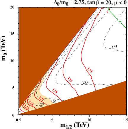
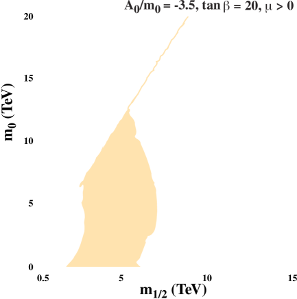
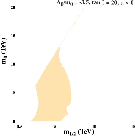
Figure 2: As in Fig. 1, but for the cases $\tan\beta=20$, $A_{0}=2.75\,m_{0}$ and $\mu>0$ (upper left panel), $\tan\beta=20$, $A_{0}=2.75\,m_{0}$ and $\mu<0$ (upper right panel), $\tan\beta=20$, $A_{0}=-3.5\,m_{0}$ and $\mu>0$ (lower left panel) and $\tan\beta=20$, $A_{0}=-3.5\,m_{0}$ and $\mu<0$ (lower right panel). Contours of $M_{h}$ calculated using FeynHiggs 2.14.1 are shown as red solid lines those using FeynHiggs 2.10.0 as thin gray dashed lines. The light orange shaded region corresponds to $M_{h}\in[122,128]~{}\mathrm{GeV}$ using FeynHiggs 2.14.1. In each panel, the X marks the position of the stop coannihilation endpoint. The solid green lines show the lower limit on the proton lifetime calculated in a minimal supersymmetric SU(5) GUT. For $A,\mu<0$, the gray shading at high $m_{1/2}$ denotes the lack of convergence of the RGEs due to a divergent $b$-quark Yukawa coupling.

We note that the green contours where $\tau(p\to K+\nu)=6.6\times 10^{33}$ yrs in the minimal SU(5) GUT model are at much larger values of $m_{1/2}$ and $m_{0}$ for $\tan\beta=20$ than they were for $\tan\beta=5$, as was also to be expected. However, we emphasize that the calculation of the proton lifetime is sensitive to the details of the GUT dynamics, and that proton stability may be an issue but is not necessarily a problem for the CMSSM with $\tan\beta=20$.

Details of the coannihilation strips and endpoints are seen more clearly in Fig. 3, which shows the profiles of the stop coannihilation strips for $\tan\beta=5$ that were shown in Fig. 1. The values of $m_{1/2}$ are indicated along the lower horizontal axes, and the corresponding values of $m_{\tilde{\chi}^{0}_{1}}$ are shown along the upper horizontal axes. For each value of $m_{1/2}$ we use SSARD to calculate the value of $m_{0}$ that yields the correct neutralino dark matter density, which we then use to calculate the other quantities shown. The left vertical axes show the scales for the mass difference $m_{\tilde{t}_{1}}-m_{\tilde{\chi}^{0}_{1}}$, which is shown as the blue curve in each panel. Here and in subsequent analogous figures, the right vertical axes are the scales for the values of $M_{h}$, the “allowed” range $M_{h}\in[122,128]~{}\mathrm{GeV}$ is indicated by the horizontal light orange shaded region. The other lines show the values of $M_{h}$ calculated using FeynHiggs 2.14.1 (solid red) and FeynHiggs 2.10.0 (dashed black). Since we assign a theoretical uncertainty of $\pm 3~{}\mathrm{GeV}$ to the FeynHiggs 2.14.1 calculation of $M_{h}$, as indicated by the light orange shaded band, the portions of the horizontal axes corresponding to the FeynHiggs 2.14.1 calculation of $M_{h}\in[122,128]~{}\mathrm{GeV}$ should be regarded as consistent with experiment.

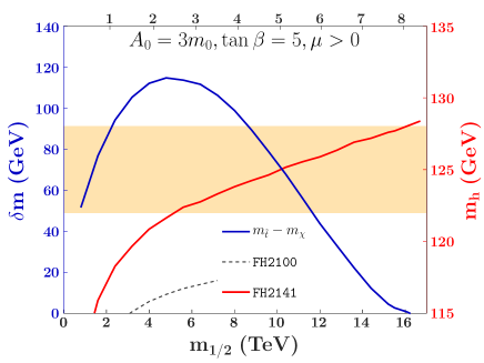
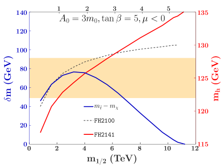
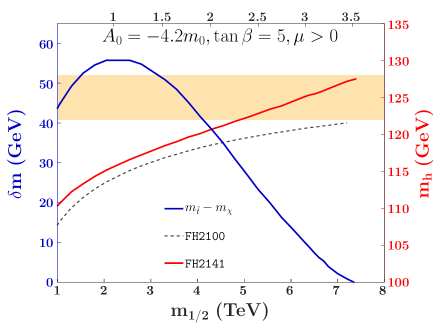
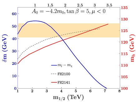
Figure 3: The profiles of the CMSSM stop coannihilation strips for $\tan\beta=5$, $A_{0}=3\,m_{0}$ and $\mu>0$ (upper left), $\tan\beta=5$, $A_{0}=3\,m_{0}$ and $\mu<0$ (upper right), $\tan\beta=5$, $A_{0}=-4.2\,m_{0}$ and $\mu>0$ (lower left), and $\tan\beta=5$, $A_{0}=-4.2\,m_{0}$ and $\mu<0$ (lower right). The lower horizontal axes show $m_{1/2}$, and the upper horizontal axes show the corresponding values of $m_{\tilde{\chi}^{0}_{1}}$ in TeV. The blue curves show the mass difference $m_{\tilde{t}_{1}}-m_{\tilde{\chi}^{0}_{1}}$, to be read from the left vertical axes. The horizontal light orange shaded band between $M_{h}=122,128~{}\mathrm{GeV}$ corresponds to predictions for $M_{h}$ that may be regarded as consistent with experiment. The other lines show the values of $M_{h}$ calculated using FeynHiggs 2.14.1 (red) and FeynHiggs 2.10.0 (dashed black), to be read from the right vertical axes.

The upper limits of the stop coannihilation strips shown in Fig. 3 range from $m_{1/2}\simeq 16~{}\mathrm{TeV}$ ($m_{\tilde{\chi}^{0}_{1}}\simeq 8~{}\mathrm{TeV}$) for $\tan\beta=5$, $A_{0}=3\,m_{0}$ and $\mu>0$ (upper left panel) down to $m_{1/2}\simeq 7.1~{}\mathrm{TeV}$ ($m_{\tilde{\chi}^{0}_{1}}\simeq 3.4~{}\mathrm{TeV}$) for $\tan\beta=5$, $A_{0}=-4.2\,m_{0}$ and $\mu<0$ (lower right panel). In the case of $\tan\beta=5$, $A_{0}=3\,m_{0}$, $\mu>0$ (upper left panel of Fig. 3), FeynHiggs 2.14.1 yields acceptable values of $M_{h}$ for $m_{\tilde{\chi}^{0}_{1}}\gtrsim 2.5~{}\mathrm{TeV}$ to the end of the strip. On the other hand, FeynHiggs 2.10.0 yielded values of $M_{h}$ that are unacceptably low for $m_{\tilde{\chi}^{0}_{1}}<4~{}\mathrm{TeV}$, and unstable values of $M_{h}$ for $m_{\tilde{\chi}^{0}_{1}}>4~{}\mathrm{TeV}$. For the other sign of $\mu$ (upper right panel of Fig. 3), both versions of FeynHiggs yield larger values of $M_{h}$, with FeynHiggs 2.14.1 now yielding acceptable values for $m_{\tilde{\chi}^{0}_{1}}\in[{1.1},2.7]~{}\mathrm{TeV}$, whereas FeynHiggs 2.10.0 would have yielded acceptable values for $m_{\tilde{\chi}^{0}_{1}}\in[{0.7},2.3]~{}\mathrm{TeV}$. The differences between the two versions of FeynHiggs are also significant for $A_{0}=-4.2\,m_{0}$ (lower panels of Fig. 3), with FeynHiggs 2.14.1 yielding acceptable values of $M_{h}$ for $m_{\tilde{\chi}^{0}_{1}}\gtrsim 2.4~{}\mathrm{TeV}$. In contrast, FeynHiggs 2.10.0 predicted a Higgs mass which was below $122$ GeV over the entire strip. When the sign of $\mu$ is reversed for this value of $A_{0}$, $m_{\tilde{\chi}^{0}_{1}}\gtrsim 2.4~{}\mathrm{TeV}$ is viable with the new version of FeynHiggs.

Fig. 4 displays an analogous set of profiles of stop coannihilation strips for $\tan\beta=20$, with $A_{0}=2.75\,m_{0}$ in the upper panels, $A_{0}=-3.5\,m_{0}$ in the lower panels, $\mu>0$ in the left panels and $\mu<0$ in the right panels. The upper limits on $m_{1/2}$ in the stop coannihilation strip imposed by $M_{h}$ range between $\mathord{\sim}\,9~{}\mathrm{TeV}$ for the case $\tan\beta=20$, $A_{0}=2.75\,m_{0}$, $\mu>0$ and $\mathord{\sim}\,5.5~{}\mathrm{TeV}$ for the case $\tan\beta=20$, $A_{0}=-3.5\,m_{0}$, $\mu<0$. As in the case of $\tan\beta=5$, the differences between FeynHiggs 2.14.1 and FeynHiggs 2.10.0 are larger for $A_{0}>0$ than for $A_{0}<0$. Values of $m_{\tilde{\chi}^{0}_{1}}$ allowed by the FeynHiggs 2.14.1 calculation of $M_{h}$ range from $\mathord{\sim}\,0.8$ to $\mathord{\sim}\,4.5~{}\mathrm{TeV}$ when $A_{0}=2.75\,m_{0}$ and $\mu>0$, $\mathord{\sim}\,0.6$ to $\mathord{\sim}\,2.2~{}\mathrm{TeV}$ when $A_{0}=2.75\,m_{0}$ and $\mu<0$, and $\mathord{\sim}\,1.3$ to $\mathord{\sim}\,2.6~{}\mathrm{TeV}$ when $A_{0}=-3.5\,m_{0}$ for both signs of $\mu$. The calculation of $M_{h}$ using FeynHiggs 2.10.0 would have favored different ranges of $m_{\tilde{\chi}^{0}_{1}}$ in general, e. g., allowing $m_{\tilde{\chi}^{0}_{1}}\gtrsim 1.3~{}\mathrm{TeV}$ for $A_{0}=2.75\,m_{0}$ and $\mu>0$. We also note that, at the larger value of $\tan\beta$ in this figure, the sign of $\mu$ plays a smaller role than in Fig. 3 with $\tan\beta=5$.

As seen in Figs. 3 and 4, in general FeynHiggs 2.14.1 yields values of $M_{h}$ that increase more rapidly with $m_{1/2}$ than the values calculated with FeynHiggs 2.10.0 along the stop coannihilation strips we have studied. As a consequence, the FeynHiggs 2.14.1 values of $M_{h}$ lie within the “allowed” range for $M_{h}$ in a smaller interval of $m_{1/2}$ in some cases. Furthermore, they tend to be larger than the FeynHiggs 2.10.0 values at large $m_{1/2}$. These differences change substantially the ranges of $m_{1/2}$ that are consistent with the experimental measurement of $M_{h}$.

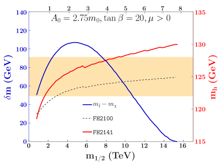
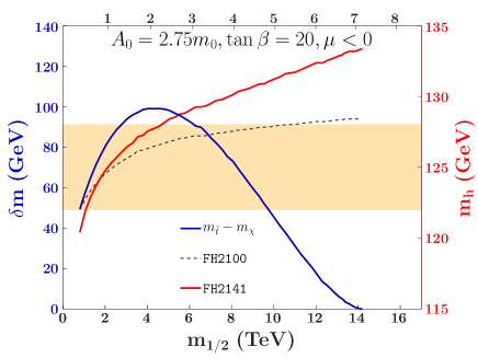
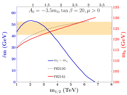
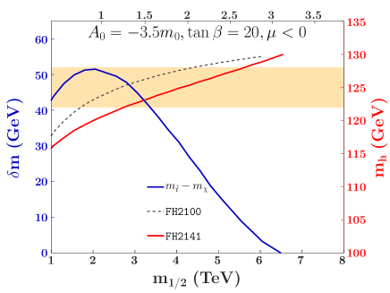
Figure 4: The profiles of the CMSSM stop coannihilation strips for $\tan\beta=20$, $A_{0}=2.75\,m_{0}$ and $\mu>0$ (upper left), $\tan\beta=20$, $A_{0}=2.75\,m_{0}$ and $\mu<0$ (upper right), $\tan\beta=20$, $A_{0}=-3.5\,m_{0}$ and $\mu>0$ (lower left), and $\tan\beta=20$, $A_{0}=-3.5\,m_{0}$ and $\mu<0$ (lower right). The lower horizontal axes show $m_{1/2}$, and the upper horizontal axes show the corresponding values of $m_{\tilde{\chi}^{0}_{1}}$ in TeV. The blue curves show the mass difference $m_{\tilde{t}_{1}}-m_{\tilde{\chi}^{0}_{1}}$, to be read from the left vertical axes. The horizontal light orange shaded band between $M_{h}=122,128~{}\mathrm{GeV}$ corresponds to predictions for $M_{h}$ that may be regarded as consistent with experiment. The other lines show the values of $M_{h}$ calculated using FeynHiggs 2.14.1 (red) and FeynHiggs 2.10.0 (dashed black), to be read from the right vertical axes.

3.1.2 Focus-Point Strips in the CMSSM

We now turn to an alternative mechanism in the CMSSM that can yield an acceptable cold dark matter density even for large values of (some) input parameters. This is the focus-point region, where the neutralino LSP acquires a significant Higgsino component that enhances (co)annihilation rates, thereby bringing the relic density down into the allowed range.

Examples of focus-point strips are visible in the $(m_{1/2},m_{0})$ planes shown in Fig. 5. The regions shaded pink in these plots are where the electroweak symmetry-breaking conditions cannot be satisfied, and the dark blue strips running along the boundaries of these regions (now clearly visible) are the focus-point strips. To make these strips more visible, we used the range $0.06<\Omega_{\chi}\,h^{2}<0.2$. As before, the brick red shaded regions are where the LSP is charged. In addition to the stau-LSP regions in the lower right parts of the planes, we see in the upper panels for $\tan\beta=10$, $A_{0}=0$ and the two signs of $\mu$ additional brick red strips where the LSP is a chargino. In the lower right panel for $\tan\beta=30$, $A_{0}=0$ and $\mu<0$ there is a gray shaded region at large $m_{1/2}$ where the RGEs for the Yukawa coupling of the $b$ quark break down. This region expands as $\tan\beta$ is increased when $\mu<0$.

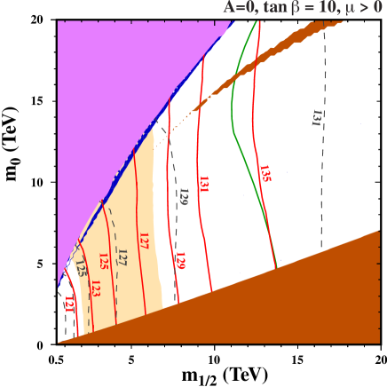
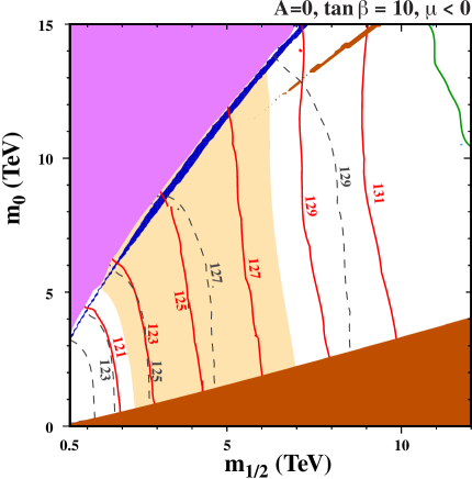
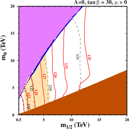
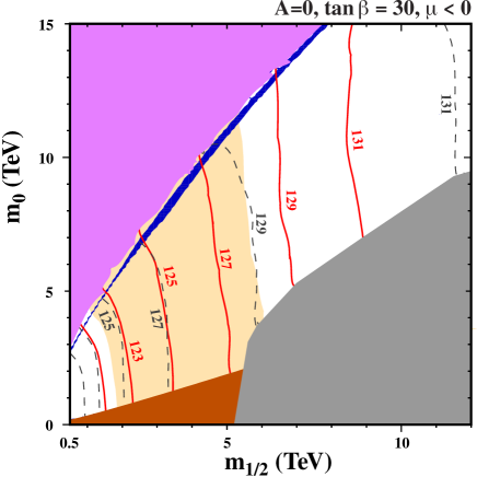
Figure 5: As in Fig. 1, but for the cases $\tan\beta=10$, $A_{0}=0$ and $\mu>0$ (upper left panel), $\tan\beta=10$, $A_{0}=0$ and $\mu<0$ (upper right panel), $\tan\beta=30$, $A_{0}=0$ and $\mu>0$ (lower left panel), and $\tan\beta=30$, $A_{0}=0$ and $\mu<0$ (lower right panel). The electroweak symmetry-breaking conditions cannot be satisfied in the regions shaded pink in these plots. Contours of $M_{h}$ calculated using FeynHiggs 2.14.1 are shown as red solid lines, those using FeynHiggs 2.10.0 as gray dashed lines. The light orange shaded region corresponds to $M_{h}\in[122,128]~{}\mathrm{GeV}$ using FeynHiggs 2.14.1. The blue strips show the region with $0.06<\Omega_{\chi}\,h^{2}<0.2$. The solid green lines show the lower limit on the proton lifetime calculated in a minimal supersymmetric SU(5) GUT. For $\tan\beta=30$, these lie beyond the range of the plot. For large $\tan\beta$ and $\mu<0$, the gray shading at high $m_{1/2}$ denotes the lack of convergence of the RGEs due to a divergent $b$-quark Yukawa coupling.

Fig. 5 displays examples of focus-point strips that extend to $m_{1/2}$ and $m_{0}\gtrsim 10~{}\mathrm{TeV}$. Although the values of $m_{\tilde{t}_{1}}-m_{\tilde{\chi}^{0}_{1}}$ can become very large along this strip, the relic density is instead controlled by the value of $\mu$, which tends towards zero as the pink region is approached. For small $\mu$, the LSP becomes Higgsino-like, and the relic density is determined by Higgsino annihilations and coannihilations with the second Higgsino and chargino, which are nearly degenerate in mass with the LSP. While the extent of the strips is very large, as one can see in each of the panels, it is limited by the Higgs mass which differs in the two versions of FeynHiggs. The profiles of these strips are shown in Fig. 6 for $\tan\beta=10$ upper panels) and $\tan\beta=30$ (lower panels), for $\mu>0$ (left panels) and for $\mu<0$ (right panels), with $A_{0}=0$ in all cases. There is little difference between the calculations of $M_{h}$ using FeynHiggs 2.14.1 (red lines) and FeynHiggs 2.10.0 (black dashed lines) for the different signs of $\mu$, with FeynHiggs 2.14.1 yielding lower $M_{h}$ for $m_{1/2}\lesssim 6$ or $7~{}\mathrm{TeV}$. As expected, the calculations generally produce higher Higgs masses for $\tan\beta=30$ than for $\tan\beta=10$, particularly at small $m_{1/2}$. In both cases the values of $M_{h}$ obtained with FeynHiggs 2.14.1 are compatible with experiment for ranges of $1.2$ to $1.5~{}\mathrm{TeV}\lesssim m_{1/2}\lesssim 5.4$ to $6.4~{}\mathrm{TeV}$, whereas the larger values of $M_{h}$ obtained with FeynHiggs 2.10.0 would have been problematic for $m_{1/2}\gtrsim 3$ or $4~{}\mathrm{TeV}$.

Fig. 5 also shows the minimal SU(5) proton decay limits (as green contours) for $\tan\beta=10$. For $\tan\beta=30$, the contour would lie beyond the scope of the plot. As a consequence, the proton decay limit is in conflict with the upper limit derived from the Higgs mass. However, we stress again that this should be viewed as a constraint on the GUT rather than a problem for the low-energy supersymmetric model.

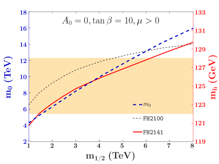
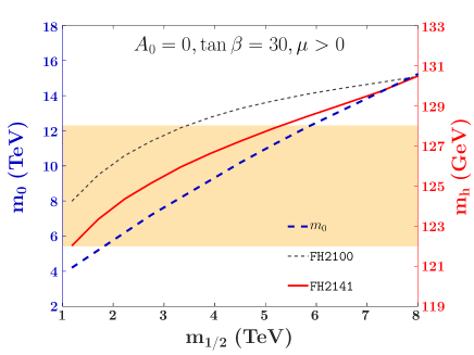
Figure 6: The profiles of the focus-point strips for $A_{0}=0$ and $\mu>0$ (left panels), $\mu<0$ (right panels) and $\tan\beta=10$ (upper panels) and $\tan\beta=30$ (lower panels). The lower horizontal axes show $m_{1/2}$, the blue dashed curves show the value of $m_{0}$, to be read from the left vertical axes. The horizontal light orange shaded band between $M_{h}=122,128~{}\mathrm{GeV}$ corresponds to predictions for $M_{h}$ that may be regarded as consistent with experiment. The other lines show the values of $M_{h}$ calculated using FeynHiggs 2.14.1 (red) and FeynHiggs 2.10.0 (dashed black), to be read from the right vertical axes.

3.2 Sub-GUT Models

We now extend the previous discussion to a ‘sub-GUT’ class of SUSY models, in which the soft SUSY-breaking parameters are universal at some input scale $M_{\mathrm{i}n}$ below the GUT scale $M_{\mathrm{G}UT}$ but above the electroweak scale [21, 17, 18]. Models in this class may arise if the soft SUSY-breaking parameters in the visible sector are induced by gluino condensation or some dynamical mechanism that becomes effective below the GUT scale. Examples of sub-GUT models include those with mirage mediation [102] of soft SUSY breaking, and certain scenarios for moduli stabilization [106].

The reduced RG running below $M_{\mathrm{i}n}$, relative to that below $M_{\mathrm{G}UT}$ in the CMSSM and related models, leads in general to SUSY spectra that are more compressed [21]. These lead, in particular, to increased possibilities for coannihilation processes. The reduced RG running also suggests a stronger lower limit on $m_{\tilde{\chi}^{0}_{1}}$, because of a smaller hierarchy to the gluino mass, and there are also smaller hierarchies between the squark and slepton masses. For a discussion of the implications for LHC searches for sparticles in sub-GUT models, see [22].

The five-dimensional parameter space of the sub-GUT MSSM that we consider here includes, besides $M_{\mathrm{i}n}$ and $\tan\beta$, the three soft supersymmetry-breaking parameters $m_{1/2}$, $m_{0}$ and $A_{0}$ that are familiar from the CMSSM, but which are now assumed to be universal at the sub-GUT input mass scale $M_{\mathrm{i}n}<M_{\mathrm{G}UT}$.

Fig. 7 illustrates some of the possibilities that appear in this five-dimensional space. The panels in the top and middle rows are all for $\tan\beta=20$, $A_{0}=2.75\,m_{0}$ and $\mu>0$, with different choices of $M_{\mathrm{i}n}=10^{7}$ GeV (top left), $10^{8}$ GeV (top right), $10^{9}$ GeV (middle left), and $10^{10}$ GeV (middle right). Similar parameter planes were considered in Ref. [20] using FeynHiggs 2.13.0. As $M_{\mathrm{i}n}$ increases, we see that a double-lobed brick red region at low $m_{1/2}$ and $m_{0}$ expands to larger mass values. The upper left lobe is a stop-LSP region, and the lower right lobe is a stau-coannihilation region. With some imagination one can anticipate that for larger $M_{\mathrm{i}n}$ the plane would evolve towards the CMSSM case shown in the upper left panel of Fig. 2, which has the same values of $\tan\beta=20$ and $A_{0}=2.75\,m_{0}$, but $M_{\mathrm{i}n}\to M_{\mathrm{G}UT}$. As in that plane, there are dark blue stop coannihilation strips that border the upper left lobes in the top and middle left panels of Fig. 7. Once again, to improve the visibility of the relic density strips, we show the values of $0.06<\Omega_{\chi}\,{h^{2}}<0.2$ in the blue shaded region with the exception of the two panels with $A_{0}=2.75\,m_{0}$ and $M_{\mathrm{i}n}=10^{9}~{}\mathrm{GeV}$ where the range $0.1151<\Omega_{\chi}\,{h^{2}}<0.1235$ is used. This is possible as the neutralino-stop mass difference varies very slowly with increasing $m_{0}$, allowing for a visible coannihilation strip.

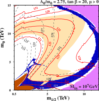
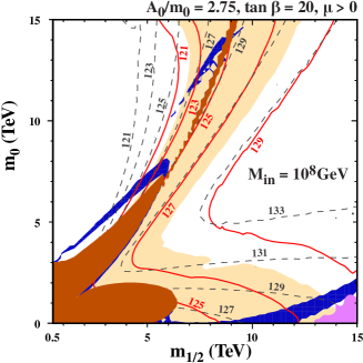
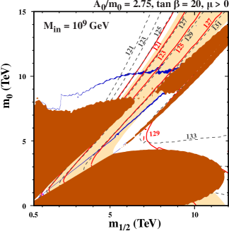
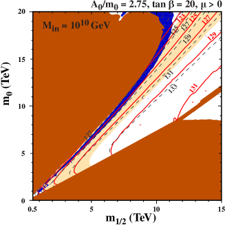
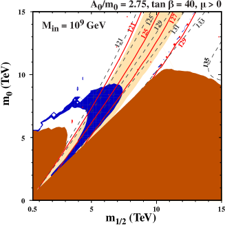
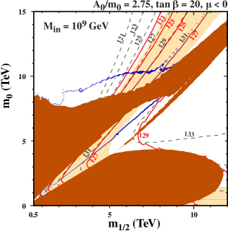
Figure 7: As in Fig. 1, but for sub-GUT scenarios with $\tan\beta=20$, $A_{0}=2.75\,m_{0}$, $M_{\mathrm{i}n}=10^{7}$ GeV (top left), $M_{\mathrm{i}n}=10^{8}$ GeV (top right), $M_{\mathrm{i}n}=10^{9}$ GeV (middle left), and $M_{\mathrm{i}n}=10^{10}$ GeV (middle right), also for $\tan\beta=40$, $A_{0}=2.75\,m_{0}$, $M_{\mathrm{i}n}=10^{9}$ GeV (bottom left), all with $\mu>0$, and $\tan\beta=20$, $A_{0}=2.75\,m_{0}$, $M_{\mathrm{i}n}=10^{9}$ GeV, $\mu<0$ (bottom right). The electroweak symmetry-breaking conditions cannot be satisfied in the regions shaded pink in these plots. Contours of $M_{h}$ calculated using FeynHiggs 2.14.1 are shown as red solid lines, those using FeynHiggs 2.10.0 as gray dashed lines. The light orange shaded region corresponds to $M_{h}\in[122,128]~{}\mathrm{GeV}$ using FeynHiggs 2.14.1. The blue strips show the region with $0.06<\Omega_{\chi}\,h^{2}<0.2$ except when $A_{0}=2.75\,m_{0}$ and $M_{\mathrm{i}n}=10^{9}~{}\mathrm{GeV}$ where $0.1151<\Omega_{\chi}\,h^{2}<0.1235$ is used.

Some other features are worth noting. In the top left panel of Fig. 7, for $M_{\mathrm{i}n}=10^{7}$ GeV, there are a pair of pink regions at large $m_{1/2}$ where the electroweak vacuum conditions cannot be satisfied, which shrinks away at larger $M_{\mathrm{i}n}$. Bordering these pink regions there is a crescent-shaped focus-point band. We also note in the top left panel for $M_{\mathrm{i}n}=10^{7}$ GeV an irregular blue ring-shaped region extending above the stop strip, and in the top right panel for $M_{\mathrm{i}n}=10^{8}$ GeV there is a blue strip that crosses a brick red chargino LSP strip when $m_{0}\sim 14~{}\mathrm{TeV}$. As discussed in Ref. [20], the masses of the three lightest neutralinos are quite similar in these regions of parameter space, and multiple coannihilations interplay, enhanced through the heavy Higgs funnel. The chargino LSP region expands when $M_{\mathrm{i}n}=10^{9}~{}\mathrm{GeV}$ (middle left) and merges with the stau-LSP region when $M_{\mathrm{i}n}=10^{10}~{}\mathrm{GeV}$ (middle right).

Contours of $M_{h}$ with values determined by FeynHiggs 2.14.1 are shown by red solid curves and determined by FeynHiggs 2.10.0 with dashed gray curves. In much of the parameter space, the FeynHiggs 2.14.1 values are lower by about $4$ GeV than the values produced by FeynHiggs 2.10.0. This difference shifts the viable regions of the parameter space, as is seen more clearly in Fig. 8, which shows the profiles along the dark matter strips in these sub-GUT scenarios. In the top left panel for $\tan\beta=20$, $A_{0}=2.75\,m_{0}$, $M_{\mathrm{i}n}=10^{7}$ GeV and $\mu>0$ we distinguish two groupings of lines, one extending up to $m_{1/2}\sim 3$ TeV, and the other from $m_{1/2}\sim 3$ TeV to $m_{1/2}\sim 12$ TeV corresponding, respectively, to the near-vertical ‘peninsula’ at low $m_{1/2}$ in Fig. 7 that extends up to $m_{0}\sim 5$ TeV and to the arc that lies close to the boundary of the region where electroweak symmetry breaking is possible. In the low-$m_{1/2}$ grouping, corresponding to the dark matter strip lying above the stop-LSP region, the blue dashed lines show that $m_{\tilde{\chi}^{0}_{1}}\lesssim 2.7~{}\mathrm{TeV}$ along these strips, and the red lines show that FeynHiggs 2.14.1 generally yields values of $M_{h}$ that are smaller than the experimental value, whereas the dashed black lines show that FeynHiggs 2.10.0 would have yielded acceptable values of $M_{h}$ on the lower-$m_{0}$ side of the ‘peninsula’ and part of the higher-$m_{0}$ side. In the high-$m_{1/2}$ grouping, the blue dashed lines show that $m_{\tilde{\chi}^{0}_{1}}\sim 1~{}\mathrm{TeV}$, which is characteristic of Higgsino dark matter. The red solid line indicates that FeynHiggs 2.14.1 yields acceptable values of $M_{h}$ along most of the lower-$m_{0}$ part of the arc up to $m_{1/2}\gtrsim 10~{}\mathrm{TeV}$, whereas it yields values of $M_{h}$ that are too high along the upper part of the arc. In contrast, FeynHiggs 2.10.0 would have yielded acceptable values of $M_{h}$ only for $m_{1/2}\lesssim 7~{}\mathrm{TeV}$ along the lower arc.

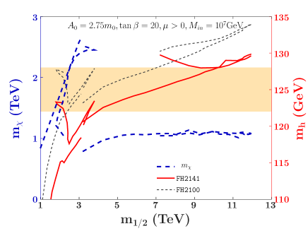
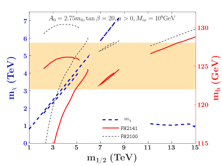
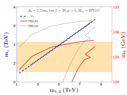
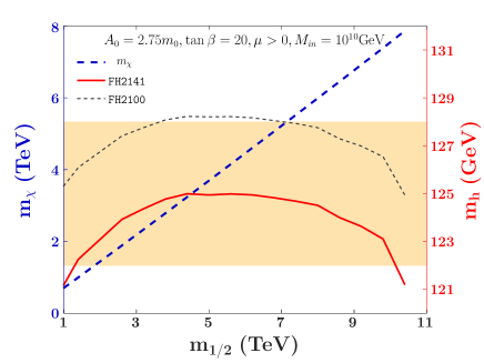
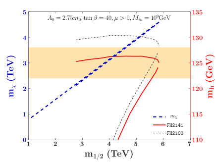
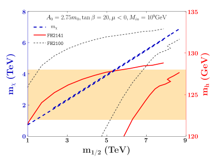
Figure 8: The profiles of the sub-GUT dark matter strips for $A_{0}=2.75\,m_{0}$ and, going from top left to bottom right, $\{M_{\mathrm{i}n}(\mathrm{GeV}),\tan\beta,{\mathrm{s}gn}\mu\}=$ $\{10^{7},20,+\}$, $\{10^{8},20,+\}$, $\{10^{9},20,+\}$, $\{10^{10},20,+\}$, $\{10^{9},40,+\}$, $\{10^{9},20,-\}$. The lower horizontal axes show $m_{1/2}$, the blue dashed curves show $m_{\tilde{\chi}^{0}_{1}}$ (left vertical axes). The “allowed” range for $M_{h}$ is indicated by the horizontal light orange shaded band for $M_{h}\in[122,128]~{}\mathrm{GeV}$. Calculated values for $M_{h}$: FeynHiggs 2.14.1 (red) and FeynHiggs 2.10.0 (dashed black), to be read from the right vertical axes.

As one can see by comparing the results in the upper four panels of Fig. 8, the strips and values of $M_{h}$ are very sensitive to $M_{\mathrm{i}n}$. For $M_{\mathrm{i}n}=10^{8}~{}\mathrm{GeV}$, the high, middle and low $m_{1/2}$ regions are clearly separate. Comparing with Fig. 7, we can associate the curves at low $m_{1/2}\lesssim 6$ TeV with the relic density strip corresponding to stop coannihilation. The higher flatter curves and the lower steeper curves represent the strips below and above the stop-LSP region respectively. The change from FeynHiggs 2.10.0 to FeynHiggs 2.14.1 lowers $M_{h}$ by a few $~{}\mathrm{GeV}$ and brings the higher strip into good agreement with experiment, while pushing the lower strip to lower values of $M_{h}$. We see that $m_{\tilde{\chi}^{0}_{1}}\lesssim 5~{}\mathrm{TeV}$ along the upper strips, but $2~{}\mathrm{TeV}\lesssim m_{\tilde{\chi}^{0}_{1}}\lesssim 4~{}\mathrm{TeV}$ along the lower strip. For the heavy-Higgs-funnel region at $m_{1/2}\sim 7$–$9~{}\mathrm{TeV}$, $m_{\tilde{\chi}^{0}_{1}}\sim 6$–$7~{}\mathrm{TeV}$. While the results of both versions of FeynHiggs are consistent with the experimental value in this region, FeynHiggs 2.14.1 decreases $M_{h}$ by $3.5~{}\mathrm{GeV}$ compared to FeynHiggs 2.10.0. The Higgsino strip at high $m_{1/2}\gtrsim 11~{}\mathrm{TeV}$ is only slightly affected by the change, but FeynHiggs 2.14.1 (unlike FeynHiggs 2.10.0) yields acceptable $M_{h}$ along much of the high-$m_{1/2}$ strip.

At $M_{\mathrm{i}n}=10^{9}~{}\mathrm{GeV}$, there is again a substantial change in $M_{h}$. The upper, flatter profiles correspond to the strip that threads between the stop- and stau-LSP regions and, in contrast with the result from FeynHiggs 2.10.0, now lies at an acceptable value of $M_{h}$ for a wide range in $m_{1/2}$. In contrast, the steeper profiles correspond to the nearly horizontal stop-coannihilation strip in Fig. 7, and are now only viable at $m_{1/2}\gtrsim 6.5~{}\mathrm{TeV}$. We see that $m_{\tilde{\chi}^{0}_{1}}\lesssim 6.6~{}\mathrm{TeV}$ along both the dark matter strips. At still larger $M_{\mathrm{i}n}=10^{10}~{}\mathrm{GeV}$, the lower strip in the previous plot has now morphed into a stop-coannihilation strip reminiscent of those in the CMSSM, which runs nearly parallel with the Higgs-mass contours. In this case we find that $m_{\tilde{\chi}^{0}_{1}}\lesssim 8~{}\mathrm{TeV}$. Both FeynHiggs 2.14.1 and FeynHiggs 2.10.0 give acceptable values of $M_{h}$ along this strip but, for most of this strip, $M_{h}$ is significantly lower and greatly improved in FeynHiggs 2.14.1.

The two bottom panels of Fig. 7 illustrate other features of the sub-GUT parameter space. The bottom left panel has $A_{0}=2.75\,m_{0}$, $M_{\mathrm{i}n}=10^{9}$ GeV and $\mu>0$ as before, but $\tan\beta=40$. Comparing with the middle left panel for $\tan\beta=20$, we see that the stop-LSP lobe has contracted whereas the stau-LSP lobe has expanded, the stop-coannihilation band has broadened, and the chargino-LSP region has disappeared. The Higgs-mass profiles in Fig. 8 in this case correspond to the two sides of the stop-coannihilation region in Fig. 7, the upper, flatter profiles corresponding to the lower strip running parallel to the Higgs-mass contours and the steeper profiles to the upper stop-coannihilation strip. While $M_{h}$ is not very sensitive to the version of FeynHiggs for the former strip, FeynHiggs 2.14.1 improves the latter by lowering $M_{h}$ by $3$–$4$ GeV. Finally, the bottom right panel has $\tan\beta=20$, $A_{0}=2.75\,m_{0}$, $M_{\mathrm{i}n}=10^{9}$ GeV and $\mu<0$. It is relatively similar to the middle left panel, which has the opposite sign of $\mu$ but identical values of the other parameters. The main difference is the appearance of a ‘causeway’ between the chargino-LSP ‘island’ and the stop-LSP lobe. We see that the results for the Higgs-mass profiles are also very similar, indicating that the sign of $\mu$ is less important than the values of the other sub-GUT parameters.

As seen in Fig. 8, in general FeynHiggs 2.14.1 yields lower values of $M_{h}$ compared to FeynHiggs 2.10.0 along both the upper and lower sub-GUT strips we have studied. In the cases of the lower-$m_{0}$ strips (solid lines) this reduction improves consistency with the experimental value of $M_{h}$ over a wider range of $m_{1/2}$. The picture is more mixed for the higher-$m_{0}$ strips, where the preferred ranges of $m_{1/2}$ change, but are not necessarily more extensive when FeynHiggs 2.14.1 is used.

3.3 Minimal AMSB Models

As a contrast to the previous CMSSM and sub-GUT models, now we analyze the minimal scenario for anomaly-mediated SUSY breaking (the mAMSB) [29, 30]. This has a very different spectrum, and a different composition of the LSP, giving sensitivity to different aspects of the calculation of $M_{h}$. The mAMSB has three relevant continuous parameters, with the overall scale of SUSY breaking being set by the gravitino mass, $m_{3/2}$. In pure AMSB the soft SUSY-breaking scalar masses $m_{0}$, like the gaugino masses, are proportional to $m_{3/2}$ before renormalization. However, in this case renormalization leads to negative squared masses for sleptons. Thus, the pure AMSB is unrealistic, and some additional contributions to the scalar masses $m_{0}$ are postulated. It is simplest to assume that these are universal, as in minimal AMSB (mAMSB) models. In the mAMSB model the soft trilinear SUSY-breaking mass terms, $A_{i}$, are determined by anomalies, like the gaugino masses, and hence are also proportional to $m_{3/2}$, resulting in the following three free continuous parameters: $m_{3/2}$, $m_{0}$ and the ratio of Higgs vevs, $\tan\beta$. The $\mu$ term and the soft Higgs bilinear SUSY-breaking term, $B$, are determined phenomenologically via the electroweak vacuum conditions, as in the CMSSM and related models, and may have either sign.

Since the gaugino masses $M_{1,2,3}$ are induced by anomalous loop effects, they are suppressed relative to the gravitino mass, $m_{3/2}$, which is quite heavy in this scenario: $m_{3/2}\gtrsim 20~{}\mathrm{TeV}$. The gaugino masses have the following ratios at NLO: $|M_{1}|:|M_{2}|:|M_{3}|\approx 2.8:1:7.1$. We note that the wino-like states are lighter than the bino, which is therefore not a candidate to be the LSP. The LSP may be either a Higgsino-like or a wino-like neutralino $\tilde{\chi}^{0}_{1}$, and is almost degenerate with a chargino partner, $\tilde{\chi}^{\pm}_{1}$, in both cases. If the LSP is a wino-like $\tilde{\chi}^{0}_{1}$ and it is the dominant source of the dark matter density, its mass has been shown to be $\mathord{\simeq}\,3~{}\mathrm{TeV}$ [107, 108] once Sommerfeld-enhancement effects [109] are taken into account. On the other hand, if a Higgsino-like $\tilde{\chi}^{0}_{1}$ provides the CDM density, $m_{\tilde{\chi}^{0}_{1}}\sim 1.1~{}\mathrm{TeV}$. In the mAMSB model, the Higgsino-like LSP still has a non-negligible wino component, and is therefore heavier than a pure Higgsino, with $m_{\chi}\gtrsim 1.5~{}\mathrm{TeV}$.

The following are characteristic features of the mAMSB model: the superpartners of the left- and right-handed leptons are nearly degenerate in mass, $m_{\tilde{\ell}_{R}}\approx m_{\tilde{\ell}_{L}}$, as are the lightest chargino and neutralino, $m_{\tilde{\chi}^{\pm}_{1}}\approx m_{\tilde{\chi}^{0}_{1}}$. The ratio between the slepton and gaugino masses depends on the input parameters, but the squark masses are typically very heavy, since they receive a contribution ${\propto}\,g_{3}^{4}\,m^{2}_{3/2}$ where $g_{3}^{2}/(4\,\pi)=\alpha_{s}$. The relatively small loop-induced values of the trilinears $A_{i}$ and the measured Higgs mass also favor relatively high stop masses.

     

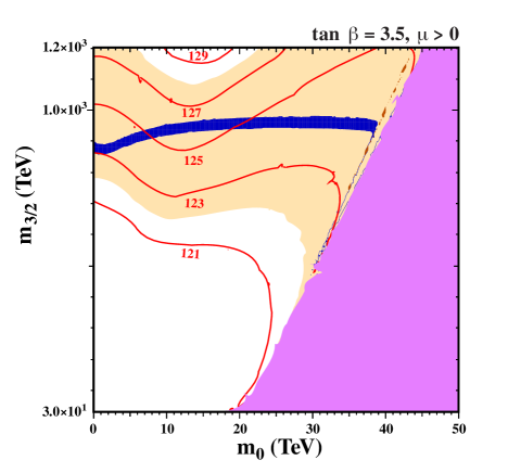
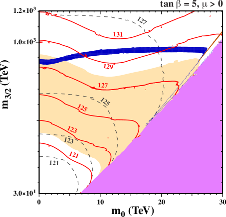
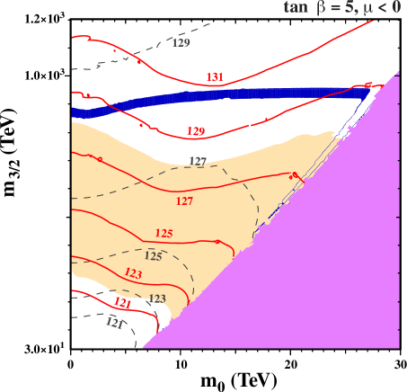
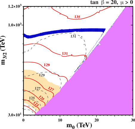
Figure 9: The $(m_{0},m_{3/2})$ planes in the mAMSB model for $\tan\beta=3.5$, $\mu>0$ (upper left panel), for $\tan\beta=5$, $\mu>0$ (upper right panel), for $\tan\beta=5$, $\mu<0$ (lower left panel), and for $\tan\beta=20$, $\mu>0$ (lower right panel). The electroweak symmetry-breaking conditions cannot be satisfied in the regions shaded pink in these plots. Contours of $M_{h}$ calculated using FeynHiggs 2.14.1 are shown as red solid lines, those using FeynHiggs 2.10.0 as gray dashed lines. The light orange shaded region corresponds to $M_{h}\in[122,128]~{}\mathrm{GeV}$ found using FeynHiggs 2.14.1. The blue strips show the region with $0.06<\Omega_{\chi}\,h^{2}<0.2$.

We display in Fig. 9 four $(m_{0},m_{3/2})$ planes in the mAMSB model. They all have a pink shaded region at large $m_{0}$ and relatively small $m_{3/2}$ where the electroweak vacuum conditions cannot be satisfied. Each panel also features a prominent near-horizontal band with acceptable dark matter density where the LSP is mainly a wino with mass $\mathord{\simeq}\,3~{}\mathrm{TeV}$. They also feature narrower and less obvious strips close to the electroweak vacuum boundary where the LSP has a larger Higgsino fraction and a smaller mass. In this figure we use the range $0.1151<\Omega_{{\chi}}\,h^{2}<0.1235$. As one can see, there is a strong preference for low $\tan\beta$ for the wino-dark-matter strip. At $\tan\beta>5$, most of the wino strip has Higgs masses in excess of $128$ GeV. While portions of the Higgsino strip are acceptable at higher $\tan\beta$, at $\tan\beta=20$ the pair of Higgsino strips is also at large $M_{h}$.

The profiles of the mAMSB-dark-matter strips displayed in Fig. 9 are shown in Fig. 10. In each panel, the horizontal axis is $m_{0}$, the left vertical axis is $m_{\tilde{\chi}^{0}_{1}}$, and the right vertical axis is $M_{h}$. We can again easily distinguish between the wino and Higgsino-like strips. The wino strip spans a wide range in $m_{0}$ as seen in Fig. 9, where the Higgsino-like strip resides only at large $m_{0}$. In the wino-like strip, the neutralino mass is shown by the blue dashed curves and $m_{\tilde{\chi}^{0}_{1}}\simeq 3~{}\mathrm{TeV}$ at large $m_{0}$, falling to $\mathord{\sim}\,2.7~{}\mathrm{TeV}$ at low $m_{0}$, whereas along the lower strip $m_{\tilde{\chi}^{0}_{1}}$ falls from $\mathord{\simeq}\,3~{}\mathrm{TeV}$ to $\mathord{\sim}\,1.5~{}\mathrm{TeV}$ as $m_{0}$ decreases towards the tip of the strip at $m_{0}\sim 15$ to $30~{}\mathrm{TeV}$.

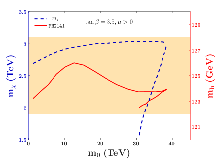
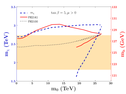
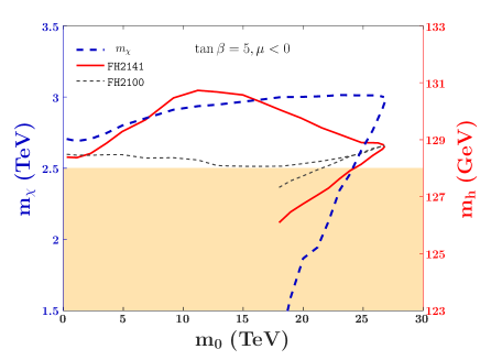
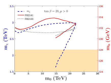
Figure 10: The profiles of the mAMSB strips for $\tan\beta=3.5$, $\mu>0$ (upper left panel), for $\tan\beta=5$, $\mu>0$ (upper right panel), for $\tan\beta=5$, $\mu<0$ (lower left panel), and for $\tan\beta=20$, $\mu>0$ (lower right panel). The lower horizontal axes show $m_{0}$, the blue dashed lines show $m_{\tilde{\chi}^{0}_{1}}$, to be read from the left vertical axes. The “allowed” range for $M_{h}$ is indicated by the horizontal light orange shaded region for $M_{h}\in[122,128]~{}\mathrm{GeV}$. Calculated values for $M_{h}$: FeynHiggs 2.14.1 (red) and FeynHiggs 2.10.0 (dashed black), to be read from the right vertical axes.

We see in the upper left panel of Fig. 10 that, for $\tan\beta=3.5$ and $\mu>0$, the Higgs mass $M_{h}$ calculated with FeynHiggs 2.14.1 (red lines) is consistent with the experimental value all along both strips, within the theoretical uncertainties. We do not show the results from FeynHiggs 2.10.0 in this case, as they were not reliable for $\tan\beta=3.5$. On the other hand, calculations of $M_{h}$ with FeynHiggs 2.14.1 are significantly higher than the experimental value along the wino-like strips in the other panels, which are for larger values of $\tan\beta$. In contrast, FeynHiggs 2.10.0 calculations of $M_{h}$ were significantly lower along the wino-like strips, and compatible with experiment for $\tan\beta=5$ and $\mu>0$. In the cases of the Higgsino-like strips, FeynHiggs 2.14.1 calculations of $M_{h}$ are compatible with experiment along that for $\tan\beta=5$ and $\mu>0$ and most of the corresponding strip for $\tan\beta=5$ and $\mu<0$, though not for the Higgsino-like strip for $\tan\beta=20$ and $\mu>0$. FeynHiggs 2.10.0 gave generally larger values of $M_{h}$ along these Higgsino-like strips, which are compatible with experiment only for the strip for $\tan\beta=5$ and $\mu>0$ and part of the strip for $\tan\beta=5$ and $\mu<0$.

In the mAMSB, as seen in Fig. 10, in general FeynHiggs 2.14.1 yields values of $M_{h}$ along the Higgsino strips that are more consistent with the experimental measurement than the ones with FeynHiggs 2.10.0. On the other hand, the values of $M_{h}$ along the wino strip are generally larger for FeynHiggs 2.14.1 than for FeynHiggs 2.10.0, and in poorer agreement with experiment. Hence, in this case the improvements in FeynHiggs 2.14.1 yield a preference for a quite different region of the model parameter space.

3.4 The pMSSM11

In contrast to the above models in which soft SUSY breaking is assumed to originate from some specific theoretical mechanism, we now study a model in which the SUSY parameters are constrained by purely phenomenological considerations. In general, such phenomenological MSSM (pMSSM) [32] models contain many more parameters. Here we consider a variant of the pMSSM with $11$ parameters fixed at the electroweak-scale, the pMSSM11, as analyzed in Ref. [34] using the available experimental constraints including many from the first LHC run at $13$ TeV. The model parameters are three independent gaugino masses, $M_{1,2,3}$, a common mass for the first-and second-generation squarks, $m_{\tilde{q}}$, a mass for the third-generation squarks, $m_{\widetilde{q}_{3}}$, that is allowed to be different, a common mass, $m_{\tilde{\ell}}$, for the first-and second-generation sleptons, a mass for the stau, $m_{\tilde{\ell}_{3}}$, that is also allowed to be different, a single trilinear mixing parameter, $A$, the Higgs mixing parameter $\mu$, the pseudoscalar Higgs mass, $M_{A}$, and the ratio of Higgs vevs, $\tan\beta$. These parameters are all fixed at a renormalization scale $M_{\mathrm{S}USY}\equiv\sqrt{m_{\tilde{t}_{1}}\,m_{\tilde{t}_{2}}}$, where $m_{\tilde{t}_{1}}$, $m_{\tilde{t}_{2}}$ are the masses of the two stop mass eigenstates. This is also the scale at which electroweak vacuum conditions are imposed. As in all the models we study, the sign of the mixing parameter $\mu$ may be either positive or negative.

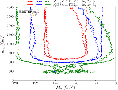
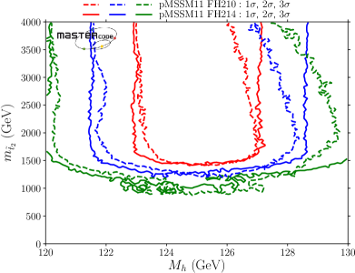
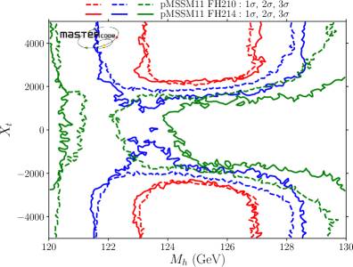
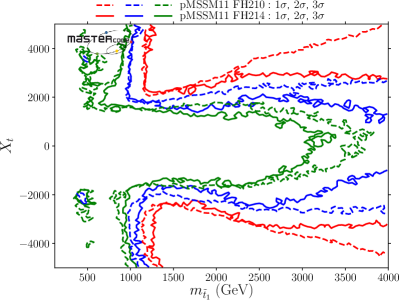
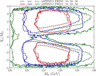
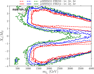
Figure 11: Explorations of the sensitivities of $M_{h}$ to $m_{\tilde{t}_{1,2}}$ in preferred regions of the pMSSM11 found

in Ref. [34], displayed in the $(M_{h},m_{\tilde{t}_{1}})$ plane (top left panel), the $(M_{h},m_{\tilde{t}_{2}})$ plane (top right panel), the $(M_{h},X_{t})$ plane (middle left panel), the $(m_{\tilde{t}_{1}},X_{t})$ plane (middle right panel), the $(M_{h},X_{t}/M_{S})$ plane (bottom left panel), and the $(m_{\tilde{t}_{1}},X_{t}/M_{S})$ plane (bottom right panel). In each panel the red, blue and green contours outline the regions favored at the $68\%$ CL (1-$\sigma$), $95\%$ CL (2-$\sigma$) and $99.7\%$ CL (3-$\sigma$), respectively, and the solid (dashed) lines are those found in a global analysis of all relevant data using FeynHiggs 2.14.1 (FeynHiggs 2.10.0) to calculate $M_{h}$.

The flexibility of the pMSSM11 model allows, in principle, many different mass hierarchies to be explored, and hence different aspects of the $M_{h}$ calculation. In particular, since the Higgs mass is most sensitive, in general, to the stop masses, we explore in Fig. 11 what stop masses and mixing are compatible with the measured Higgs mass, without being constrained by any preconceived theoretical ideas such as those arising in the models discussed in the previous sections. In each panel of Fig. 11, the regions favored at the $68\%$ CL (1-$\sigma$), $95\%$ CL (2-$\sigma$) and $99.7\%$ CL (3-$\sigma$) are enclosed by red, blue and green contours, respectively, which are shown solid (dashed) if FeynHiggs 2.14.1 (FeynHiggs 2.10.0) is used to calculate the $\chi^{2}$ contribution the LHC measurement of $M_{h}$ to a frequentist global analysis of the pMSSM11 parameter space [34].

We see in the top left panel of Fig. 11 that the experimental value of $M_{h}$ can be accommodated by values of $m_{\tilde{t}_{1}}\gtrsim 500$ GeV ($1000$ GeV) ($1300$ GeV) at the $99.7$ ($95$) ($68$)% CL, whether FeynHiggs 2.14.1 or FeynHiggs 2.10.0 is used to calculate $M_{h}$. The most significant difference is a tendency for FeynHiggs 2.10.0 to disfavor larger values of $M_{h}$ when $m_{\tilde{t}_{1}}$ is large, a tendency that is absent when FeynHiggs 2.14.1 is used. We note also that the likelihood function is quite flat for $m_{\tilde{t}_{1}}\gtrsim 1500~{}\mathrm{GeV}$, and for this reason we do not quote a best-fit point. The upper right panel shows that values of $m_{\tilde{t}_{2}}\gtrsim 1$ ($1.3$) ($1.5$) TeV are favored at the $99.7$ ($95$) ($68$)% CL, again with little difference between the results with FeynHiggs 2.14.1 and FeynHiggs 2.10.0. Again, FeynHiggs 2.10.0 tends to disfavor larger values of $M_{h}$ when $m_{\tilde{t}_{2}}$ is large, but not FeynHiggs 2.14.1.

The middle panels of Fig. 11 explore the sensitivities of the $M_{h}$ calculation to the stop mixing parameter $X_{t}\equiv A_{t}-\mu\cot\beta$ in the two versions of FeynHiggs . We see that they both favor values of $\lvert X_{t}\rvert\gtrsim 2$ TeV, though $X_{t}=0$ is allowed at the $99.7\%$ CL. However, we see in the middle right panel that this is possible only for $m_{\tilde{t}_{1}}\gtrsim 3$ ($3.5$) TeV when FeynHiggs 2.14.1 (FeynHiggs 2.10.0) is used. This behavior at $X_{t}=0$ may be the origin of the often-repeated statement that the measured value of $M_{h}$ requires a large stop mass. In fact, as already mentioned above, the upper panels of Fig. 11 show that $M_{h}\simeq 125$ GeV is quite compatible with $m_{\tilde{t}_{1}}\sim 1.2$ TeV, and the middle right panel shows that this is possible if $\lvert X_{t}\rvert\sim 2$ TeV. The bottom plots of Fig. 11 show the same results as in the middle row, but with $X_{t}/M_{S}$ on the vertical axes. In particular, in the lower right plot it can clearly be seen that the correct Higgs-boson mass prediction requires either large mixing in the stop sector, or large scalar top masses. Here small mixing can more easily be reached with FeynHiggs 2.14.1.

Fig. 12 contains one-dimensional plots of the global $\chi^{2}$-likelihood functions for $m_{\tilde{t}_{1}}$ (left panel) and $X_{t}/M_{S}$ (right panel), shown as solid (dashed) lines as found using FeynHiggs 2.14.1 (FeynHiggs 2.10.0) to calculate the $\chi^{2}$ contribution from the LHC measurement of $M_{h}$. Here we see again that the global minima are at $m_{\tilde{t}_{1}}\sim 1.5$ TeV and $|X_{t}/M_{S}|\sim 2$, with little difference between FeynHiggs 2.14.1 and FeynHiggs 2.10.0. The $\chi^{2}$ function for $m_{\tilde{t}_{1}}$ rises very mildly as $m_{\tilde{t}_{1}}$ approaches $4$ TeV, and the exact location of the minimum value cannot be regarded as significant. We note also the appearance of a secondary minimum with $\Delta\chi^{2}<3$ when $m_{\tilde{t}_{1}}\simeq 500$ GeV. The $\chi^{2}$ function for $X_{t}/M_{S}$ exhibits no significant sign preference, but disfavors $X_{t}=0$ by $\Delta\chi^{2}\simeq 4$ if FeynHiggs 2.14.1 is used, compared to $\Delta\chi^{2}\simeq 8$ with FeynHiggs 2.10.0.

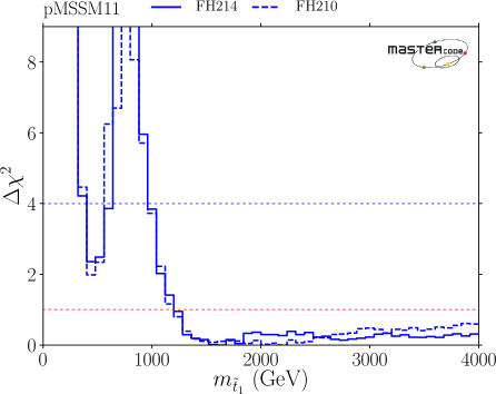
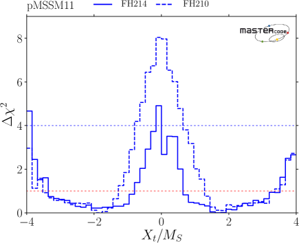
Figure 12: The one-dimensional global $\Delta\chi^{2}$ functions for $m_{\tilde{t}_{1}}$ (left panel) and $X_{t}/M_{S}$ (right panel), as found using FeynHiggs 2.14.1 (FeynHiggs 2.10.0) to calculate the $\chi^{2}$ contribution from the LHC measurement of $M_{h}$, shown as solid (dashed) lines.

Overall, in the pMSSM11 we see no clear trend towards lower or higher values of $M_{h}$ when going from FeynHiggs 2.10.0 to FeynHiggs 2.14.1. Although individual parameter choices may yield different values for $M_{h}$, the experimental constraints on the pMSSM11 favor regions in the parameter space where marginalization to minimize $\chi^{2}$ yields milder effects on the light ${\cal CP}$-even Higgs-boson mass.

4 Conclusions

We have investigated the physics implications of improved Higgs-boson mass predictions in the MSSM, comparing results from FeynHiggs 2.14.1 and FeynHiggs 2.10.0. The main differences, as discussed in this paper, are $3$-loop RG effects and $2$-loop threshold corrections that can accommodate three separate mass scales: $m_{\tilde{q}}$, $m_{\tilde{g\,}\!}$ and an electroweakino mass scale, as well as an improved treatment of $\overline{\mathrm{DR}}$ input parameters in the scalar top sector avoiding problems with the conversion to on-shell parameters, that yields significant improvements for large SUSY-breaking scales. These changes reflect the progress made over the last $\mathord{\sim}\,5$ years in “hybrid” Higgs-mass calculations in the MSSM.

The examples presented in this paper illustrate how the preferred ranges of the parameter space of the MSSM can change when FeynHiggs 2.14.1 is used to calculate $M_{h}$, as compared to when FeynHiggs 2.10.0 is used. The first representative model is the CMSSM. As is well known, in the CMSSM reproducing the correct CDM density of neutralinos, despite the rising lower limits on sparticle masses from the LHC, tends to favor narrow strips of parameter space that extend to large $m_{1/2}$ and/or $m_{0}$.The improvements in FeynHiggs 2.14.1 can play important roles in these parameter regions. Examples of these high-mass strips include some where stop coannihilation is important, and others where the focus-point mechanism is operative. In both these cases, using FeynHiggs 2.14.1 rather than FeynHiggs 2.10.0 changes significantly the parts of the strips that are consistent with the experimental measurement of $M_{h}$. This reflects the different dependences on $m_{1/2}$ of the FeynHiggs 2.14.1 and FeynHiggs 2.10.0 calculations of $M_{h}$.

We have also studied sub-GUT models, in which the soft SUSY-breaking masses are assumed to be universal at some scale $M_{\mathrm{i}n}$ below the conventional grand unification scale $M_{\mathrm{G}UT}$ assumed in the CMSSM. Both the stop-coannihilation and focus-point mechanisms may be operational in different regions of the sub-GUT parameter space. Depending on the choice of $M_{\mathrm{i}n}$, the forms of the DM strips can be very different from those allowed in the CMSSM, with the possibility of two (or more) DM strips with different values of $m_{0}$ for the same value of $m_{1/2}$. In general, along the lower-$m_{0}$ strips the agreement between FeynHiggs 2.14.1 calculations of $M_{h}$ and experiment is better than that for the FeynHiggs 2.10.0 calculations.

As a third case we investigated the mAMSB, where two different classes of DM strips occur: one where the LSP may be mainly a wino, or one where it may have a large Higgsino component. Both of these types of dark-matter strips extend to relatively large values of $m_{0}$, with an LSP mass $\mathord{\sim}\,3~{}\mathrm{TeV}$ or $\mathord{\gtrsim}\,1~{}\mathrm{TeV}$, respectively. Calculations of $M_{h}$ using FeynHiggs 2.14.1 favor the Higgsino region, whereas calculations using FeynHiggs 2.10.0 favored the wino region.

In the case of the pMSSM11, we find little change in the regions of parameter space favored by $M_{h}$, which can be ascribed to the fact that there is no big mass hierarchy. The predictions from both FeynHiggs 2.14.1 and FeynHiggs 2.10.0 are consistent with $M_{h}\simeq 125~{}\mathrm{GeV}$ and $m_{\tilde{t}_{1}}\sim 1.3~{}\mathrm{TeV}$ at the $68\%$ CL, and they both allow $m_{\tilde{t}_{1}}\sim 500~{}\mathrm{GeV}$ with $\Delta\chi^{2}\sim 3$. Both versions of FeynHiggs disfavor small stop mixing, $X_{t}=0$, by $\Delta\chi^{2}\sim 4\ (8)$ in the case of FeynHiggs 2.14.1 (FeynHiggs 2.10.0), with $|X_{t}/M_{S}|\sim 2$ being favored. Obtaining the correct prediction for the Higgs-boson mass requires either large mixing in the scalar top sector (with $|X_{t}/M_{S}|\sim 2$), or large scalar top masses, though smaller values of $|X_{t}/M_{S}|$ can be reached more easily with FeynHiggs 2.14.1. We find no clear preference towards lower or higher values of $M_{h}$ when going from FeynHiggs 2.10.0 to FeynHiggs 2.14.1 in the pMSSM11. The experimental constraints yield parameter combinations with mild effects on the light ${\cal CP}$-even Higgs-boson mass after marginalization to minimize $\chi^{2}$.

In conclusion, we comment that in this paper we have limited ourselves to exploratory studies, and have not attempted to make global fits to the parameters of any of the SUSY models we have discussed. However, we find an overall tendency towards better compatibility with the experimental data when employing the updated Higgs-boson mass calculations. Performing new fits with updated calculations of $M_{h}$ would clearly be an interesting next step, and we hope that the studies described here will give some insight into the results to be expected from such more complete investigations.

Acknowledgments

The work of JE was supported in part by the United Kingdom STFC Grant ST/P000258/1, and in part by the Estonian Research Council via a Mobilitas Pluss grant. The work of SH was supported in part by the MEINCOP (Spain) under contract FPA2016-78022-P, in part by the Spanish Agencia Estatal de Investigación (AEI), in part by the EU Fondo Europeo de Desarrollo Regional (FEDER) through the project FPA2016-78645-P, in part by the “Spanish Red Consolider MultiDark” FPA2017-90566-REDC, and in part by the AEI through the grant IFT Centro de Excelencia Severo Ochoa SEV-2016-0597. The work of KAO was supported in part by DOE grant DE-SC0011842 at the University of Minnesota. The work of SP was supported by the ANR grant “HiggsAutomator” (ANR-15-CE31-0002). The work of HR was partially funded by the Danish National Research Foundation, grant number DNRF90. The work of JZ was supported by KAKENHI Grant Number JP26104009.

References

- [1] G. Aad et al. [ATLAS Collaboration], Phys. Lett. B 716 (2012) 1 [arXiv:1207.7214 [hep-ex]].
- [2] S. Chatrchyan et al. [CMS Collaboration], Phys. Lett. B 716 (2012) 30 [arXiv:1207.7235 [hep-ex]].
- [3] H. P. Nilles, Phys. Rept. 110 (1984) 1.
- [4] H. E. Haber and G. L. Kane, Phys. Rept. 117 (1985) 75.
- [5] S. Heinemeyer, O. Stål and G. Weiglein, Phys. Lett. B 710 (2012) 201 [arXiv:1112.3026 [hep-ph]].
- [6] H. E. Haber and R. Hempfling, Phys. Rev. Lett. 66 (1991) 1815.
- [7] J. R. Ellis, G. Ridolfi and F. Zwirner, Phys. Lett. B 257 (1991) 83.
- [8] Y. Okada, M. Yamaguchi and T. Yanagida, Prog. Theor. Phys. 85 (1991) 1.
- [9] G. Aad et al. [ATLAS and CMS Collaborations], Phys. Rev. Lett. 114 (2015) 191803 [arXiv:1503.07589 [hep-ex]].
- [10] G. Aad et al. [ATLAS and CMS Collaborations], JHEP 1608 (2016) 045 [arXiv:1606.02266 [hep-ex]].
- [11] O. Buchmueller et al., Eur. Phys. J. C 74 (2014) no.3, 2809 [arXiv:1312.5233 [hep-ph]].
- [12] T. Hahn, S. Heinemeyer, W. Hollik, H. Rzehak and G. Weiglein, Phys. Rev. Lett. 112 (2014) no.14, 141801 [arXiv:1312.4937 [hep-ph]].
- [13] H. Goldberg, Phys. Rev. Lett. 50 (1983) 1419.
- [14] J. Ellis, J. Hagelin, D. Nanopoulos, K. Olive, M. Srednicki, Nucl. Phys. B 238 (1984) 453.
- [15] H. Bahl et al., IFT–UAM/CSIC–18-095.
- [16] M. Drees and M. M. Nojiri, Phys. Rev. D 47 (1993) 376 [arXiv:hep-ph/9207234]; G. L. Kane, C. F. Kolda, L. Roszkowski and J. D. Wells, Phys. Rev. D 49 (1994) 6173 [arXiv:hep-ph/9312272]; J. R. Ellis, K. A. Olive, Y. Santoso and V. C. Spanos, Phys. Lett. B 565 (2003) 176 [arXiv:hep-ph/0303043]; H. Baer and C. Balazs, JCAP 0305, 006 (2003) [arXiv:hep-ph/0303114]; A. B. Lahanas and D. V. Nanopoulos, Phys. Lett. B 568, 55 (2003) [arXiv:hep-ph/0303130]; U. Chattopadhyay, A. Corsetti and P. Nath, Phys. Rev. D 68, 035005 (2003) [arXiv:hep-ph/0303201]; J. Ellis and K. A. Olive, arXiv:1001.3651 [astro-ph.CO], published in Particle dark matter, ed. G. Bertone, pp. 142-163.
- [17] J. Ellis, F. Luo, K. A. Olive and P. Sandick, Eur. Phys. J. C 73, no. 4, 2403 (2013) [arXiv:1212.4476 [hep-ph]].
- [18] J. Ellis, J. L. Evans, F. Luo, N. Nagata, K. A. Olive and P. Sandick, Eur. Phys. J. C 76, no. 1, 8 (2016) [arXiv:1509.08838 [hep-ph]].
- [19] J. Ellis, J. L. Evans, A. Mustafayev, N. Nagata and K. A. Olive, Eur. Phys. J. C 76, no. 11, 592 (2016) [arXiv:1608.05370 [hep-ph]].
- [20] J. Ellis, J. L. Evans, F. Luo, K. A. Olive and J. Zheng, Eur. Phys. J. C 78 (2018) no.5, 425 [arXiv:1801.09855 [hep-ph]].
- [21] J. R. Ellis, K. A. Olive and P. Sandick, Phys. Lett. B 642 (2006) 389 [hep-ph/0607002], JHEP 0706 (2007) 079 [arXiv:0704.3446 [hep-ph]] and JHEP 0808 (2008) 013 [arXiv:0801.1651 [hep-ph]].
- [22] J. C. Costa et al., Eur. Phys. J. C 78 (2018) no.2, 158 [arXiv:1711.00458 [hep-ph]].
- [23] C. Boehm, A. Djouadi and M. Drees, Phys. Rev. D 62, 035012 (2000) [arXiv:hep-ph/9911496]; J. R. Ellis, K. A. Olive and Y. Santoso, Astropart. Phys. 18, 395 (2003) [arXiv:hep-ph/0112113]; J. L. Diaz-Cruz, J. R. Ellis, K. A. Olive and Y. Santoso, JHEP 0705, 003 (2007) [arXiv:hep-ph/0701229]; I. Gogoladze, S. Raza and Q. Shafi, Phys. Lett. B 706, 345 (2012) [arXiv:1104.3566 [hep-ph]]; M. A. Ajaib, T. Li and Q. Shafi, Phys. Rev. D 85, 055021 (2012) [arXiv:1111.4467 [hep-ph]]; J. Harz, B. Herrmann, M. Klasen, K. Kovarik and Q. L. Boulc’h, Phys. Rev. D 87 (2013) 5, 054031 [arXiv:1212.5241]; J. Harz, B. Herrmann, M. Klasen and K. Kovarik, Phys. Rev. D 91 (2015) 3, 034028 [arXiv:1409.2898 [hep-ph]]; A. Ibarra, A. Pierce, N. R. Shah and S. Vogl, Phys. Rev. D 91, no. 9, 095018 (2015) [arXiv:1501.03164 [hep-ph]].
- [24] J. Edsjö, M. Schelke, P. Ullio and P. Gondolo, JCAP 0304, 001 (2003) [hep-ph/0301106].
- [25] J. Ellis, K. A. Olive and J. Zheng, Eur. Phys. J. C 74 (2014) 2947 [arXiv:1404.5571 [hep-ph]].
- [26] O. Buchmueller, M. Citron, J. Ellis, S. Guha, J. Marrouche, K. A. Olive, K. de Vries and J. Zheng, Eur. Phys. J. C 75, no. 10, 469 (2015) [arXiv:1505.04702 [hep-ph]].
- [27] S. Raza, Q. Shafi and C. S. Ün, Phys. Rev. D 92, no. 5, 055010 (2015) [arXiv:1412.7672 [hep-ph]].
- [28] J. L. Feng, K. T. Matchev and T. Moroi, Phys. Rev. Lett. 84, 2322 (2000) [arXiv:hep-ph/9908309]; H. Baer, T. Krupovnickas, S. Profumo and P. Ullio, JHEP 0510 (2005) 020 [hep-ph/0507282]; J. L. Feng, K. T. Matchev and D. Sanford, Phys. Rev. D 85, 075007 (2012) [arXiv:1112.3021 [hep-ph]]; P. Draper, J. Feng, P. Kant, S. Profumo and D. Sanford, Phys. Rev. D 88, 015025 (2013) [arXiv:1304.1159 [hep-ph]].
- [29] M. Dine and D. MacIntire, Phys. Rev. D 46, 2594 (1992) [hep-ph/9205227]; L. Randall and R. Sundrum, Nucl. Phys. B 557, 79 (1999) [arXiv:hep-th/9810155]; G. F. Giudice, M. A. Luty, H. Murayama and R. Rattazzi, JHEP 9812, 027 (1998) [arXiv:hep-ph/9810442]; A. Pomarol and R. Rattazzi, JHEP 9905, 013 (1999) [hep-ph/9903448]; J. A. Bagger, T. Moroi and E. Poppitz, JHEP 0004, 009 (2000) [arXiv:hep-th/9911029]; P. Binetruy, M. K. Gaillard and B. D. Nelson, Nucl. Phys. B 604, 32 (2001) [arXiv:hep-ph/0011081].
- [30] T. Gherghetta, G. Giudice and J. Wells, Nucl. Phys. B 559 (1999) 27 [arXiv:hep-ph/9904378]; E. Katz, Y. Shadmi and Y. Shirman, JHEP 9908, 015 (1999) [hep-ph/9906296]; Z. Chacko, M. A. Luty, I. Maksymyk and E. Ponton, JHEP 0004, 001 (2000) [hep-ph/9905390]; J. L. Feng and T. Moroi, Phys. Rev. D 61, 095004 (2000) [hep-ph/9907319]; G. D. Kribs, Phys. Rev. D 62, 015008 (2000) [hep-ph/9909376]; U. Chattopadhyay, D. K. Ghosh and S. Roy, Phys. Rev. D 62, 115001 (2000) [hep-ph/0006049]; I. Jack and D. R. T. Jones, Phys. Lett. B 491, 151 (2000) [hep-ph/0006116]; H. Baer, J. K. Mizukoshi and X. Tata, Phys. Lett. B 488, 367 (2000) [hep-ph/0007073]; A. Datta, A. Kundu and A. Samanta, Phys. Rev. D 64, 095016 (2001) [hep-ph/0101034]; H. Baer, R. Dermisek, S. Rajagopalan and H. Summy, JCAP 1007, 014 (2010) [arXiv:1004.3297 [hep-ph]]; A. Arbey, A. Deandrea and A. Tarhini, JHEP 1105, 078 (2011) [arXiv:1103.3244 [hep-ph]]; B. C. Allanach, T. J. Khoo and K. Sakurai, JHEP 1111, 132 (2011) [arXiv:1110.1119 [hep-ph]]; A. Arbey, A. Deandrea, F. Mahmoudi and A. Tarhini, Phys. Rev. D 87, no. 11, 115020 (2013) [arXiv:1304.0381 [hep-ph]].
- [31] E. Bagnaschi et al., Eur. Phys. J. C 77 (2017) no.4, 268 [arXiv:1612.05210 [hep-ph]].
- [32] See, for example, C. F. Berger, J. S. Gainer, J. L. Hewett and T. G. Rizzo, JHEP 0902, 023 (2009) [arXiv:0812.0980 [hep-ph]]; S. S. AbdusSalam, B. C. Allanach, F. Quevedo, F. Feroz and M. Hobson, Phys. Rev. D 81, 095012 (2010) [arXiv:0904.2548 [hep-ph]]; J. A. Conley, J. S. Gainer, J. L. Hewett, M. P. Le and T. G. Rizzo, Eur. Phys. J. C 71, 1697 (2011) [arXiv:1009.2539 [hep-ph]]; J. A. Conley, J. S. Gainer, J. L. Hewett, M. P. Le and T. G. Rizzo, [arXiv:1103.1697 [hep-ph]]; S. Sekmen, S. Kraml, J. Lykken, F. Moortgat, S. Padhi, L. Pape, M. Pierini and H. B. Prosper et al., JHEP 1202 (2012) 075 [arXiv:1109.5119 [hep-ph]]; A. Arbey, M. Battaglia and F. Mahmoudi, Eur. Phys. J. C 72 (2012) 1847 [arXiv:1110.3726 [hep-ph]]; A. Arbey, M. Battaglia, A. Djouadi and F. Mahmoudi, Phys. Lett. B 720 (2013) 153 [arXiv:1211.4004 [hep-ph]]; M. W. Cahill-Rowley, J. L. Hewett, A. Ismail and T. G. Rizzo, Phys. Rev. D 88 (2013) 3, 035002 [arXiv:1211.1981 [hep-ph]].
- [33] S. S. AbdusSalam, et al., Eur. Phys. J. C 71 (2011) 1835 [arXiv:1109.3859 [hep-ph]];
- [34] E. Bagnaschi et al., Eur. Phys. J. C 78 (2018) no.3, 256 [arXiv:1710.11091 [hep-ph]].
- [35] S. Heinemeyer, Int. J. Mod. Phys. A 21 (2006) 2659 [hep-ph/0407244].
- [36] S. Heinemeyer, W. Hollik and G. Weiglein, Phys. Rept. 425 (2006) 265 [hep-ph/0412214].
- [37] A. Djouadi, Phys. Rept. 459 (2008) 1 [hep-ph/0503173].
- [38] P. Draper and H. Rzehak, Phys. Rept. 619, 1 (2016) [arXiv:1601.01890 [hep-ph]].
- [39] S. Heinemeyer, W. Hollik and G. Weiglein, Phys. Rev. D 58 (1998) 091701 [hep-ph/9803277].
- [40] S. Heinemeyer, W. Hollik and G. Weiglein, Phys. Lett. B 440 (1998) 296 [hep-ph/9807423].
- [41] S. Heinemeyer, W. Hollik and G. Weiglein, Eur. Phys. J. C 9 (1999) 343 [hep-ph/9812472].
- [42] R. J. Zhang, Phys. Lett. B 447 (1999) 89 [hep-ph/9808299].
- [43] J. R. Espinosa and R. J. Zhang, JHEP 0003 (2000) 026 [hep-ph/9912236].
- [44] G. Degrassi, P. Slavich and F. Zwirner, Nucl. Phys. B 611 (2001) 403 [hep-ph/0105096].
- [45] J. R. Espinosa and R. J. Zhang, Nucl. Phys. B 586 (2000) 3 [hep-ph/0003246].
- [46] A. Brignole, G. Degrassi, P. Slavich and F. Zwirner, Nucl. Phys. B 631 (2002) 195 [hep-ph/0112177].
- [47] A. Brignole, G. Degrassi, P. Slavich and F. Zwirner, Nucl. Phys. B 643 (2002) 79 [hep-ph/0206101].
- [48] S. Heinemeyer, W. Hollik, H. Rzehak and G. Weiglein, Eur. Phys. J. C 39 (2005) 465 [hep-ph/0411114].
- [49] A. Dedes, G. Degrassi and P. Slavich, Nucl. Phys. B 672 (2003) 144 [hep-ph/0305127].
- [50] S. Heinemeyer, W. Hollik, H. Rzehak and G. Weiglein, Phys. Lett. B 652, 300 (2007) [arXiv:0705.0746 [hep-ph]].
- [51] W. Hollik and S. Passehr, Phys. Lett. B 733, 144 (2014) [arXiv:1401.8275 [hep-ph]].
- [52] W. Hollik and S. Passehr, JHEP 1410, 171 (2014) [arXiv:1409.1687 [hep-ph]].
- [53] S. Passehr and G. Weiglein, Eur. Phys. J. C 78 (2018) no.3, 222 [arXiv:1705.07909 [hep-ph]].
- [54] R. Hempfling, Phys. Rev. D 49 (1994) 6168.
- [55] L. J. Hall, R. Rattazzi and U. Sarid, Phys. Rev. D 50 (1994) 7048 [hep-ph/9306309].
- [56] M. Carena, M. Olechowski, S. Pokorski and C. E. M. Wagner, Nucl. Phys. B 426 (1994) 269 [hep-ph/9402253].
- [57] M. Carena, D. Garcia, U. Nierste and C. E. M. Wagner, Nucl. Phys. B 577 (2000) 88 [hep-ph/9912516].
- [58] D. Noth and M. Spira, Phys. Rev. Lett. 101 (2008) 181801 [arXiv:0808.0087 [hep-ph]].
- [59] D. Noth and M. Spira, JHEP 1106 (2011) 084 [arXiv:1001.1935 [hep-ph]].
- [60] S. Borowka, T. Hahn, S. Heinemeyer, G. Heinrich and W. Hollik, Eur. Phys. J. C 74 (2014) no.8, 2994 [arXiv:1404.7074 [hep-ph]].
- [61] S. P. Martin, Phys. Rev. D 71 (2005) 016012 [hep-ph/0405022].
- [62] G. Degrassi, S. Di Vita and P. Slavich, Eur. Phys. J. C 75 (2015) no.2, 61 [arXiv:1410.3432 [hep-ph]].
- [63] S. Borowka, T. Hahn, S. Heinemeyer, G. Heinrich and W. Hollik, Eur. Phys. J. C 75 (2015) no.9, 424 [arXiv:1505.03133 [hep-ph]].
- [64] S. Borowka, S. Passehr and G. Weiglein, arXiv:1802.09886 [hep-ph].
- [65] R. Barbieri, M. Frigeni and F. Caravaglios, Phys. Lett. B 258 (1991) 167.
- [66] J. R. Espinosa and M. Quiros, Phys. Lett. B 266 (1991) 389.
- [67] J. A. Casas, J. R. Espinosa, M. Quiros and A. Riotto, Nucl. Phys. B 436 (1995) 3 [Erratum: Nucl. Phys. B 439 (1995) 466] [hep-ph/9407389].
- [68] H. E. Haber and R. Hempfling, Phys. Rev. D 48 (1993) 4280 [hep-ph/9307201].
- [69] M. Carena, J. R. Espinosa, M. Quiros and C. E. M. Wagner, Phys. Lett. B 355 (1995) 209 [hep-ph/9504316].
- [70] M. Carena, M. Quiros and C. E. M. Wagner, Nucl. Phys. B 461 (1996) 407 [hep-ph/9508343].
- [71] H. E. Haber, R. Hempfling and A. H. Hoang, Z. Phys. C 75 (1997) 539 [hep-ph/9609331].
- [72] M. Carena, H. E. Haber, S. Heinemeyer, W. Hollik, C. E. M. Wagner and G. Weiglein, Nucl. Phys. B 580 (2000) 29 [hep-ph/0001002].
- [73] G. Degrassi, S. Heinemeyer, W. Hollik, P. Slavich and G. Weiglein, Eur. Phys. J. C 28 (2003) 133 [hep-ph/0212020].
- [74] S. P. Martin, Phys. Rev. D 75 (2007) 055005 [hep-ph/0701051].
- [75] P. Draper, G. Lee and C. E. M. Wagner, Phys. Rev. D 89 (2014) no.5, 055023 [arXiv:1312.5743 [hep-ph]].
- [76] E. Bagnaschi, G. F. Giudice, P. Slavich and A. Strumia, JHEP 1409 (2014) 092 [arXiv:1407.4081 [hep-ph]].
- [77] J. Pardo Vega and G. Villadoro, JHEP 1507 (2015) 159 [arXiv:1504.05200 [hep-ph]].
- [78] E. Bagnaschi, J. Pardo Vega and P. Slavich, Eur. Phys. J. C 77 (2017) no.5, 334 [arXiv:1703.08166 [hep-ph]].
- [79] E. Bagnaschi, A. Voigt and G. Weiglein, in preparation.
- [80] P. Athron, M. Bach, D. Harries, T. Kwasnitza, J. h. Park, D. Stöckinger, A. Voigt and J. Ziebell, Comput. Phys. Commun. 230 (2018) 145 doi:10.1016/j.cpc.2018.04.016 [arXiv:1710.03760 [hep-ph]].
- [81] G. Lee and C. E. M. Wagner, Phys. Rev. D 92 (2015) no.7, 075032 [arXiv:1508.00576 [hep-ph]].
- [82] E. Bagnaschi, F. Brümmer, W. Buchmüller, A. Voigt and G. Weiglein, JHEP 1603 (2016) 158 [arXiv:1512.07761 [hep-ph]].
- [83] P. Athron, J. h. Park, D. Stöckinger and A. Voigt, Comput. Phys. Commun. 190 (2015) 139 [arXiv:1406.2319 [hep-ph]].
- [84] H. Bahl and W. Hollik, Eur. Phys. J. C 76 (2016) no.9, 499 [arXiv:1608.01880 [hep-ph]].
- [85] H. Bahl, S. Heinemeyer, W. Hollik and G. Weiglein, Eur. Phys. J. C 78 (2018) no.1, 57 [arXiv:1706.00346 [hep-ph]].
- [86] S. Heinemeyer, W. Hollik and G. Weiglein, Comput. Phys. Commun. 124 (2000) 76 [hep-ph/9812320].
- [87] T. Hahn, S. Heinemeyer, W. Hollik, H. Rzehak and G. Weiglein, Comput. Phys. Commun. 180 (2009) 1426.
- [88] M. Frank, T. Hahn, S. Heinemeyer, W. Hollik, H. Rzehak and G. Weiglein, JHEP 0702 (2007) 047 [hep-ph/0611326].
- [89] For a regularly updated portal, see www.feynhiggs.de .
- [90] H. Bahl and W. Hollik, arXiv:1805.00867 [hep-ph].
- [91] S. P. Martin, Phys. Rev. D 66 (2002) 096001 [hep-ph/0206136].
- [92] S. P. Martin, Phys. Rev. D 67 (2003) 095012 [hep-ph/0211366].
- [93] R. V. Harlander, P. Kant, L. Mihaila and M. Steinhauser, Phys. Rev. Lett. 100 (2008) 191602 [Phys. Rev. Lett. 101 (2008) 039901] [arXiv:0803.0672 [hep-ph]].
- [94] P. Kant, R. V. Harlander, L. Mihaila and M. Steinhauser, JHEP 1008 (2010) 104 [arXiv:1005.5709 [hep-ph]].
- [95] R. V. Harlander, J. Klappert and A. Voigt, Eur. Phys. J. C 77 (2017) no.12, 814 [arXiv:1708.05720 [hep-ph]].
- [96] P. Athron, J. h. Park, T. Steudtner, D. Stöckinger and A. Voigt, JHEP 1701 (2017) 079 [arXiv:1609.00371 [hep-ph]].
- [97] F. Staub and W. Porod, Eur. Phys. J. C 77 (2017) no.5, 338 [arXiv:1703.03267 [hep-ph]].
- [98] B. C. Allanach and A. Voigt, arXiv:1804.09410 [hep-ph].
- [99] R. V. Harlander, J. Klappert, A. D. Ochoa and A. Voigt, arXiv:1807.03509 [hep-ph].
- [100] W. Hollik and S. Passehr, Eur. Phys. J. C 75 (2015) no.7, 336 [arXiv:1502.02394 [hep-ph]].
- [101] T. Hahn and S. Passehr, Comput. Phys. Commun. 214 (2017) 91 [arXiv:1508.00562 [hep-ph]].
- [102] C. Csaki, in M. Shifman et al. (eds.), From fields to strings, vol. 2, pp967-1060, [hep-ph/0404096]; K. Choi, A. Falkowski, H. P. Nilles and M. Olechowski, Nucl. Phys. B 718 (2005) 113 [arXiv:hep-th/0503216]; K. Choi, K. S. Jeong and K. i. Okumura, JHEP 0509 (2005) 039 [arXiv:hep-ph/0504037]; M. Endo, M. Yamaguchi and K. Yoshioka, Phys. Rev. D 72 (2005) 015004 [arXiv:hep-ph/0504036]; A. Falkowski, O. Lebedev and Y. Mambrini, JHEP 0511 (2005) 034 [arXiv:hep-ph/0507110]; R. Kitano and Y. Nomura, Phys. Lett. B 631 (2005) 58 [arXiv:hep-ph/0509039]; R. Kitano and Y. Nomura, Phys. Rev. D 73 (2006) 095004 [arXiv:hep-ph/0602096]; A. Pierce and J. Thaler, JHEP 0609 (2006) 017 [arXiv:hep-ph/0604192]; K. Kawagoe and M. M. Nojiri, [arXiv:hep-ph/0606104]; H. Baer, E.-K. Park, X. Tata and T. T. Wang, JHEP 0608 (2006) 041 [arXiv:hep-ph/0604253]; K. Choi, K. Y. Lee, Y. Shimizu, Y. G. Kim and K. i. Okumura, JCAP 0612 (2006) 017 [arXiv:hep-ph/0609132]; O. Lebedev, V. Lowen, Y. Mambrini, H. P. Nilles and M. Ratz, JHEP 0702 (2007) 063 [arXiv:hep-ph/0612035].
- [103] Information about this code is available from K. A. Olive: it contains important contributions from J. Evans, T. Falk, A. Ferstl, G. Ganis, F. Luo, A. Mustafayev, J. McDonald, K. A. Olive, P. Sandick, Y. Santoso, V. Spanos, M. Srednicki and J. Zheng.
- [104] N. Aghanim et al. [Planck Collaboration], arXiv:1807.06209 [astro-ph.CO].
- [105] J. L. Evans, N. Nagata and K. A. Olive, Phys. Rev. D 91, 055027 (2015) [arXiv:1502.00034 [hep-ph]].
- [106] S. Kachru, R. Kallosh, A. D. Linde and S. P. Trivedi, Phys. Rev. D 68, 046005 (2003) [hep-th/0301240].
- [107] J. Hisano, S. Matsumoto, M. Nagai, O. Saito and M. Senami, Phys. Lett. B 646 (2007) 34 [hep-ph/0610249].
- [108] M. Cirelli, A. Strumia and M. Tamburini, Nucl. Phys. B 787 (2007) 152 [arXiv:0706.4071 [hep-ph]]; A. Hryczuk, R. Iengo and P. Ullio, JHEP 1103 (2011) 069 [arXiv:1010.2172 [hep-ph]]; M. Beneke, A. Bharucha, F. Dighera, C. Hellmann, A. Hryczuk, S. Recksiegel and P. Ruiz-Femenia, JHEP 1603 (2016) 119 [arXiv:1601.04718 [hep-ph]].
- [109] A. Sommerfeld, Ann. Phys. 403, (1931) 257.