Fast Exact Bayesian Inference for Sparse Signals in the Normal Sequence Model

Abstract

We consider exact algorithms for Bayesian inference with model selection priors (including spike-and-slab priors) in the sparse normal sequence model. Because the best existing exact algorithm becomes numerically unstable for sample sizes over $n=500$, there has been much attention for alternative approaches like approximate algorithms (Gibbs sampling, variational Bayes, etc.), shrinkage priors (e.g. the Horseshoe prior and the Spike-and-Slab LASSO) or empirical Bayesian methods. However, by introducing algorithmic ideas from online sequential prediction, we show that exact calculations are feasible for much larger sample sizes: for general model selection priors we reach n=25 000, and for certain spike-and-slab priors we can easily reach n=100 000. We further prove a de Finetti-like result for finite sample sizes that characterizes exactly which model selection priors can be expressed as spike-and-slab priors. The computational speed and numerical accuracy of the proposed methods are demonstrated in experiments on simulated data, on a differential gene expression data set, and to compare the effect of multiple hyper-parameter settings in the beta-binomial prior. In our experimental evaluation we compute guaranteed bounds on the numerical accuracy of all new algorithms, which shows that the proposed methods are numerically reliable whereas an alternative based on long division is not.

Keywords: spike-and-slab prior, model selection, high-dimensional statistics

1 Introduction

In the sparse normal sequence model we observe a sequence $Y=(Y_{1},...,Y_{n})$ that satisfies

$$Y_{i}=\theta_{i}+\varepsilon_{i},\quad i=1,\ldots,n,$$ (1)

for independent standard normal random variables $\varepsilon_{i}$, where $\theta=(\theta_{1},...,\theta_{n})$ is the unknown signal of interest. It is assumed that the number of non-zero signal components $s$ in $\theta$ is small compared to the size of the whole sample (i.e. $s=o(n)$). Applications of this model include detecting differentially expressed genes [45, 36, 39, 56, 23], bankruptcy prediction for publicly traded companies using Altman’s Z-score in finance [2, 3], separation of the background and source in astronomical images [18, 28], and wavelet analysis [1, 31]. The model is further of interest to sanity check (approximate) inference methods for the more general sparse linear regression model (see [17] and references therein), which reduces to the normal sequence model when the design is the identity matrix.

The sparse normal sequence model, which is also called the sparse normal means model, has been extensively studied from a frequentist perspective (see, for instance, [27, 7, 1]), but here we consider Bayesian approaches, which endow $\theta$ with a prior distribution. This prior serves as a natural way to introduce sparsity into the model and the corresponding posterior can be used for model comparison and uncertainty quantification (see [24, 53, 37, 5] and references therein). One natural and well-understood class of priors are model selection priors that take the following hierarchical form:

1. First a sparsity level $s$ is chosen from a prior $\pi_{n}$ on $\{0,1,...,n\}$.

2. Then, given $s$, a subset of nonzero coordinates $\mathcal{S}\subset\{0,1,\ldots,n\}$ of size $|\mathcal{S}|=s$ is selected uniformly at random.

3. Finally, given $s$ and $\mathcal{S}$, the means $\theta_{\mathcal{S}}=(\theta_{i})_{i\in\mathcal{S}}$ corresponding to the nonzero coordinates in $\mathcal{S}$ are endowed with a prior $G_{\mathcal{S}}$, while the remaining coefficients $\theta_{\mathcal{S}^{\textnormal{c}}}=(\theta_{i})_{i\notin\mathcal{S}}$ are set to zero.

As is common, we will choose the prior $G_{\mathcal{S}}$ on the nonzero coordinates in a factorized form; i.e. $\theta_{i}\sim G$ for all $i\in\mathcal{S}$, where $G$ is a fixed one-dimensional prior, which we assume to have a density $g$ (with respect to the Lebesgue measure). Under suitable conditions on $\pi_{n}$ and $G$, the posterior has good frequentist properties and contracts around the true parameter at the minimax rate, as shown by Castillo and Van der Vaart [16]. Notably, they require the prior $\pi_{n}$ to decrease at an exponential rate.

A special case of the model selection priors are the spike-and-slab priors developed by Mitchell and Beauchamp [42], George and McCulloch [26], where the coefficients of $\theta$ are assigned prior probabilities

$$\begin{split}\theta_{i}\mid\alpha&~{}\sim~{}(1-\alpha)\delta_{0}+\alpha G,\qquad i=1,...,n,\\ \alpha&~{}\sim~{}\Lambda_{n},\end{split}$$ (2)

with $\delta_{0}$ the Dirac-delta measure at $0$ (a spike) and $G$ the same one-dimensional prior as above (called the slab in this context). The a priori likelihood of nonzero coefficients is controlled by the mixing parameter $\alpha\in[0,1]$, and finally $\Lambda_{n}$ is a hyper-prior on $\alpha$. A typical choice for $\Lambda_{n}$ is the beta distribution: $\alpha\sim\operatorname{Beta}(\kappa,\lambda)$. In this case the prior on the sparsity level in the model selection formulation takes the form $\pi_{n}(s)=\binom{n}{s}\frac{B(\kappa+s,\lambda+n-s)}{B(\kappa,\lambda)}$, where $B(\kappa,\lambda)$ denotes the beta function with parameters $\kappa$ and $\lambda$. The resulting prior is called the beta-binomial prior. A natural choice is $\kappa=\lambda=1$ [54], which corresponds to a uniform prior on $\alpha$, but this choice does not satisfy the exponential decrease condition on $\pi_{n}$. Castillo and Van der Vaart therefore propose $\kappa=1$ and $\lambda=n+1$, which does satisfy their exponential decrease condition [16, Example 2.2], and in Section 5 we confirm empirically that the latter indeed leads to better posterior estimates for $\theta$.

Model selection priors set certain signal components to zero, which is desirable for model selection, but makes computation of the posterior difficult since the number of possible sets $\mathcal{S}$ is exponentially large (i.e. $2^{n}$). Castillo and Van der Vaart [16] do provide an exact algorithm, based on multiplication of polynomials (see Appendix A), but this algorithm runs into numerical problems for sample sizes over $n=250$ or sometimes $n=500$ (see Section 3) and it also requires $O(n^{3})$ computation steps, which makes it too slow to handle large $n$.

The computational difficulty of model selection priors has given rise to a variety of alternative priors based on shrinkage. These include the horseshoe prior [11], for which multiple scalable implementations are available [58, 30]. The corresponding posterior achieves the minimax contraction rate and, under mild conditions, also provides reliable uncertainty quantification [61, 59, 60]. The posterior median and draws from the horseshoe posterior are not sparse, but one can use it for model selection after post-processing the posterior. An alternative is to replace the spike in the spike-and-slab prior with a Laplace distribution with very small variance, as in the Spike-and-Slab LASSO [48]. One can efficiently compute the maximum a posteriori (MAP) estimator of the corresponding posterior distribution by convex optimization.

Another way to deal with the computational problems for model selection priors is to consider approximations. The available options include Stochastic Search Variable Selection (SSVS) [26], variational Bayes approximation [64], Langevin Markov Chain Monte Carlo [44], Expectation Maximization [50], Hamiltonian Monte Carlo [53] or empirical Bayes methods [31, 40, 6].

In this paper we return to the goal of exactly computing the posterior for model selection priors, without changing the prior or introducing approximations. In Section 2 we propose a new approach based on a representation of model selection priors by a Hidden Markov Model (HMM) that comes from the literature on online sequential prediction and data compression [63], for which we can apply the standard Forward-Backward algorithm [46]. The computational complexity of this algorithm is $O(n^{2})$. To appreciate the speed-up compared to $O(n^{3})$ run time, see Section 4, where this method runs in under $15$ minutes while the previous algorithm of Castillo and Van der Vaart would take approximately $20$ days. Furthermore, in Section 2.2 we specialize to spike-and-slab priors and introduce an even faster algorithm based on a discretization of the $\alpha$ hyper-parameter, which has only $O(n^{3/2})$ run time. Using results from online sequential prediction [20], we show that this discretization provides an accurate approximation of the posterior that can be made exact to arbitrary precision, provided that the density of $\Lambda_{n}$ varies sufficiently slowly. Our conditions do not directly allow $\kappa$ or $\lambda$ to depend on $n$ in the beta-binomial prior, so we provide an extra result to cover the important case that $\kappa=1$ and $\lambda=n+1$.

Our two new approaches allow us to easily handle data sets of size $n=25\,000$ for general model selection priors and $n=100\,000$ for the subclass of spike-and-slab priors with sufficiently regular $\Lambda_{n}$, which both substantially exceed the earlier limit of $n=500$. These results are obtained on a standard laptop within a maximum time limit of half an hour. Run times for larger sample sizes can be estimated by extrapolating from Figure 2.

In Section 2.3 we further derive sufficient and necessary conditions to decide whether a model selection prior can be written in the more efficient spike-and-slab form. Since the distribution of the binary indicators for whether $\theta_{i}=0$ or not is exchangeable under the model selection priors, this amounts to a finite sample de Finetti result for a restricted class of exchangeable distributions.

In Section 3, we demonstrate the scalability and numerical accuracy of the proposed methods on simulated data. We also show there that our deterministic algorithm can be used as a benchmark to test the accuracy of approximation methods: we compare the approximate posterior from Gibbs sampling and variational Bayes to the exact posterior computed by our algorithm, which shows the surprisingly limited number of decimal places to which their answers are reliable. Then, in Section 4, we compare our methods to other approaches suggested in the literature in an application to differential gene expression for Ulcerative Colitis and Crohn’s Disease. In Section 5 we further use our new algorithms to empirically investigate the importance of the exponential decrease condition on $\pi_{n}$ by varying the hyper-parameters $\kappa$ and $\lambda$ of the beta-binomial prior. We find that exponential decrease is not just a sufficient condition for minimax posterior contraction, but it also leads to better posterior estimates of $\theta$. The paper is concluded by Section 6, where we discuss possible extensions of our algorithms.

In addition to the main paper, we provide an accompanying R package that implements our new methods [62], and supplementary material with several appendices. In Appendix A we first recall the exact algorithm by Castillo and Van der Vaart [16]. We show how to resolve its numerical stability issues by performing all intermediate computations in a logarithmic representation. The bottleneck then becomes its computational complexity, because it requires $O(n^{3})$ steps, which is prohibitive for large $n$. Two natural ideas to speed up the algorithm have been proposed by [16, 12], one based on fast polynomial multiplication and one based on long division. Surprisingly, although both approaches look very promising in theory, it turns out that neither of them works well in practice: the theoretical speed-ups for fast polynomial multiplication turn out to be so asymptotic that they do not provide significant gains for any reasonable $n$; and the long division approach becomes numerically unstable again. In Appendix B we provide an additional variation on an experiment from Section 5. Finally, Appendix C contains all proofs.

2 Exact Algorithms for Model Selection Priors

In this section we propose novel, exact algorithms for computing (marginal statistics of) the posterior distribution corresponding to model selection priors. For general model selection priors we propose a model selection HMM algorithm, and for spike-and-slab priors we introduce a faster method based on discretization of the $\alpha$ hyper-parameter. The section is concluded with a characterization of the subclass of model selection priors that can be expressed in the more efficient spike-and-slab form.

Marginal Statistics

We are interested in computing the marginal posterior probabilities that the coordinates of $\theta$ are nonzero:

$$q_{n,i}:=\Pi_{n}(\theta_{i}\neq 0\mid Y)\quad\text{for $i=1,\ldots,n$.}$$

These are sufficient to compute any other marginal statistics of interest, because, conditionally on whether $\theta_{i}$ is $0$ or not, the pair $(Y_{i},\theta_{i})$ is independent of all other pairs $(Y_{j},\theta_{j})_{j\neq i}$. For instance, the marginal posterior means can be expressed as

$$\operatorname*{\mathbb{E}}[\theta_{i}\mid Y]=q_{n,i}\operatorname*{\mathbb{E}}[\theta_{i}\mid Y_{i},\theta_{i}\neq 0]=q_{n,i}\,\frac{\zeta(Y_{i})}{\psi(Y_{i})},$$

where $\psi(y)=\int\phi(y-t)g(t)\,\textnormal{d}t$ is the slab density and $\zeta(y)=\int t\phi(y-t)g(t)\,\textnormal{d}t$, with $\phi$ the standard normal density. We may also obtain marginal quantiles by inverting the marginal posterior distribution functions

$$\Pi_{n}(\theta_{i}\leq u\mid Y)=(1-q_{n,i})\ind_{u\geq 0}+q_{n,i}\frac{\psi(Y_{i},u)}{\psi(Y_{i})},$$

where $\psi(y,u)=\int_{-\infty}^{u}\phi(y-t)g(t)\,\textnormal{d}t$. In particular, the marginal medians correspond to

$$\hat{\theta}^{\textnormal{med}}_{i}=\Big{[}H_{n,i}^{-1}\Big{(}\frac{1}{2q_{n,i}}\Big{)}\operatorname{\wedge}0\Big{]}+\Big{[}H_{n,i}^{-1}\Big{(}1-\frac{1}{2q_{n,i}}\Big{)}\operatorname{\vee}0\Big{]},$$

where $H_{n,i}^{-1}$ is the inverse of the function $H_{n,i}(u)=\frac{\psi(Y_{i},u)}{\psi(Y_{i})}$ and we use the conventions that $H_{n,i}^{-1}(v)=-\infty$ for $v\leq 0$ and $H_{n,i}^{-1}(v)=\infty$ for $v\geq 1$, see [16].

2.1 The Model Selection HMM Algorithm

Our first computationally efficient approach is based on a Hidden Markov Model (HMM) that comes from the literature on online sequential prediction and data compression [63]. This approach makes it possible to reliably compute all marginal posterior probabilities $q_{n,i}$ in only $O(n^{2})$ operations for any model selection prior.

Figure 1: The model selection prior as a Hidden Markov Model

To define the HMM, we will encode the subset of nonzero coordinates $\mathcal{S}\subset\{0,1,\ldots,n\}$ as a binary vector $B=(B_{1},\ldots,B_{n})$, where $B_{i}=1$ if $i\in\mathcal{S}$ and $B_{i}=0$ otherwise. The crucial observation is that the conditional probabilities of the model selection prior

$$\Pi_{n}(B_{i+1}\mid B_{1},\ldots,B_{i})=\Pi_{n}(B_{i+1}\mid M_{i})$$ (3)

only depend on the total number of nonzeros $M_{i}=\sum_{j=1}^{i}B_{j}\in\{0,\ldots,i\}$ in the first $i$ coordinates and not on the locations of these coordinates. We can use this observation to interpret the model selection prior as the model selection HMM shown in Figure 1, where each hidden state $H_{i}=(B_{i},M_{i})$ contains sufficient information to compute both the transition probabilities

$$P(H_{i+1}\mid H_{i})=\begin{cases}\Pi_{n}(B_{i+1}\mid M_{i})&\text{if $M_{i+1}=M_{i}+B_{i+1}$,}\\ 0&\text{otherwise,}\end{cases}$$

and the conditional distribution of $\theta_{i}$ given $H_{i}$:

$$\theta_{i} =0\quad(\text{a.s.}) B_{i}=0$$ if ,

$$\theta_{i} \sim G B_{i}=1$$ if .

In fact, in our implementation we will integrate out $\theta_{i}$ to directly obtain the conditional density

$$p(Y_{i}\mid H_{i})=\begin{cases}\phi(Y_{i})&\text{if $B_{i}=0$,}\\ \psi(Y_{i})&\text{if $B_{i}=1$.}\end{cases}$$

(Note that $\psi(Y_{i})$ is the conditional density of observation $Y_{i}$ for slabs, while $\phi(Y_{i})$ is the density of $Y_{i}$ for spikes.) Finally, the initial probabilities of $H_{1}$ are

$$P(H_{1})=\begin{cases}\Pi_{n}(B_{1})&\text{if $M_{1}=B_{1}$,}\\ 0&\text{otherwise.}\end{cases}$$

We note that the sequence of hidden states $H_{1},\ldots,H_{n}$ is in one-to-one correspondence with $\mathcal{S}$. Consequently, since the model selection HMM expresses the same joint distribution on $H_{1},\ldots,H_{n}$ as the model selection prior, and the conditional distribution of $\theta$ and $Y$ given $H_{1},\ldots,H_{n}$ is also the same, it follows that the model selection HMM is equivalent to the corresponding model selection prior.

What we gain is that, for HMMs, standard efficient algorithms are available, whose run times depend on the number of state transitions with nonzero probabilities $P(H_{i+1}\mid H_{i})$ [46]. For our purposes, we will use the Forward-Backward algorithm to compute $\Pi_{n}(H_{i}\mid Y)$ for all $i$ in $O(n^{2})$ steps, from which we can obtain $q_{n,i}=\Pi_{n}(B_{i}=1\mid Y)$ for all $i$ in another $O(n^{2})$ steps by marginalizing. For numerical accuracy, we perform all calculations using the logarithmic representation discussed in Appendix A.2.

Let $Y_{a}^{b}=(Y_{a},\ldots,Y_{b})$. Then the Forward phase in this algorithm computes the densities $p(Y_{1}^{i},H_{i}=h_{i})$ from $p(Y_{1}^{i-1},H_{i-1}=h_{i-1})$ for all $i=1,\ldots,n$ and all values $h_{i}$ of the hidden states using the recursion

$$p(Y_{1}^{i},h_{i})=\begin{cases}p(Y_{1}\mid h_{1})P(h_{1})&\text{for $i=1$,}\\ \displaystyle p(Y_{i}\mid h_{i})\sum_{h_{i-1}}p(Y_{1}^{i-1},h_{i-1})P(h_{i}\mid h_{i-1})&\text{for $1<i\leq n$.}\end{cases}$$

After the Forward phase, the Forward-Backward algorithm performs the Backward phase, which computes $p(Y_{i+1}^{n}\mid H_{i}=h_{i})$ from $p(Y_{i+2}^{n}\mid H_{i+1}=h_{i+1})$ for all $i=n,\ldots,1$ using the recursion

$$p(Y_{i+1}^{n}\mid h_{i})=\begin{cases}1&\text{for $i=n$,}\\ \displaystyle\sum_{h_{i+1}}p(Y_{i+2}^{n}\mid h_{i+1})p(Y_{i+1}\mid h_{i+1})P(h_{i+1}\mid h_{i})&\text{for $1\leq i<n$.}\end{cases}$$

Combining the results from the Forward and Backward phases, we can compute

$$\Pi_{n}(h_{i}\mid Y)\propto p(Y_{1}^{i},h_{i})p(Y_{i+1}^{n}\mid h_{i})$$

for all $i$ and $h_{i}$ as desired.

The HMM described here was introduced by [63] for the $\operatorname{Beta}(1/2,1/2)$-binomial prior (i.e. the spike-and-slab prior with $\Lambda_{n}=\operatorname{Beta}(1/2,1/2)$) in the context of the Switching Method for data compression. See [35] for an overview of many variations on this HMM. Indeed, for any $\operatorname{Beta}(\kappa,\lambda)$-binomial prior this HMM is particularly natural, because the transition probabilities of the hidden states have a closed-form expression:

$$\Pi_{n}(B_{i+1}=1\mid B_{1},\ldots,B_{i})=\Pi_{n}(B_{i+1}=1\mid M_{i})=\frac{\kappa+M_{i}}{\kappa+\lambda+i}.$$

Here we add the observations that, even when the conditional probabilities $\Pi_{n}(B_{i+1}\mid B_{1},\ldots,B_{i})$ are not available in closed form for a given model selection prior, they still satisfy (3) and can be efficiently obtained from

$$\Pi_{n}(B_{i+1}\mid B_{1},\ldots,B_{i})=\frac{v_{i+1}(M_{i}+B_{i+1})}{v_{i}(M_{i})},$$

where $v_{i}(m)=\Pi_{n}(B_{1}=b_{1},\ldots,B_{i}=b_{i})$ is the joint probability of any sequence $b_{1},\ldots,b_{i}$ with $m$ ones. These joint probabilities can be pre-computed for $i=n,\ldots,1$ in $O(n^{2})$ steps using the recursion

$$v_{i}(m)=\begin{cases}\pi_{n}(m)/\binom{n}{m}&\text{for $i=n$,}\\ v_{i+1}(m)+v_{i+1}(m+1)&\text{for $1\leq i<n$.}\end{cases}$$

Thus we can calculate the marginal posterior probabilities in $O(n^{2})$ steps for any model selection prior, not just for beta-binomial priors. The numerical accuracy of this algorithm is demonstrated in Section 3.

2.2 A Faster Algorithm for Spike-and-Slab Priors

In this section we restrict our attention to the spike-and-slab subclass of model selection priors, for which we propose further speed-ups. It is intuitively clear that the mixing hyper-parameter $\alpha$ plays a key role in the behavior of the prior distribution. The optimal choice of $\alpha$ heavily depends on the sparsity parameter $s$ of the model. For instance in case of Cauchy slabs the optimal oracle choice $\alpha=(s/n)\sqrt{\log(n/s)}$ results in minimax posterior contraction [16] and reliable uncertainty quantification [15] in $\ell_{2}$-norm. However, in practice the sparsity level $s$ is (typically) not known in advance. Therefore one cannot use the optimal oracle choice for $\alpha$. In [16] it was also shown that by choosing $\alpha=1/n$ the posterior contracts around the truth at the nearly optimal rate $s\log(n)$. This seemingly solves the problem of choosing the tuning hyper-parameter. However, a related simulation study in [16] shows that hard-thresholding at the corresponding $\sqrt{2\log(n)}$ level pairs up with substantially worse practical performance; see Tables 1 and 2 in [16]. Furthermore, in view of [15] the choice of $\alpha=1/n$ imposes too strong prior assumptions, resulting in overly small posterior spread which leads to unreliable Bayesian uncertainty quantification, i.e. the frequentist coverage of the $\ell_{2}$-credible set will tend to zero.

Therefore in practice one has to consider a data driven (adaptive) choice of the hyper-parameter $\alpha$. A computationally appealing approach is the empirical Bayes method, where the maximum marginal likelihood estimator is plugged into the posterior. The corresponding posterior mean achieves a (nearly) minimax convergence rate [31], and for slab distributions with polynomial tails the corresponding posterior contracts around the truth at the optimal rate [13]. However for light-tailed slabs (e.g. Laplace) the empirical Bayes posterior distribution will achieve a highly suboptimal contraction rate around the truth; see again [13].

Another standard (and from a Bayesian perspective more natural) approach is to endow the hyper-parameter $\alpha$ with another layer of prior $\Lambda_{n}$. However, computational problems may arise using standard Gibbs sampling techniques for sampling from the posterior; see Section 3.2 for a demonstration of this problem on a simulated data set. In the literature various speed-ups were proposed. One can for instance focus on relevant sub-sequences of the sequential parameter $\theta$ and apply the Gibbs sampler only on them. Another approach is to apply the Hamiltonian Monte Carlo method, see for instance [53]. However, none of these approaches provides an easy way to quantify their approximation error when run for a finite number of iterations. In the next section we propose a deterministic algorithm to approximate the marginal posterior probabilities $q_{n,i}$ for spike-and-slab priors, with a guaranteed bound on its approximation error that can be made arbitrarily close to zero.

2.2.1 Approximation via Discretization of the Mixing Parameter

For general model selection priors the fast HMM algorithm from Section 2.1 requires $O(n^{2})$ steps. However, for the special case of spike-and-slab priors we can do even better: we can approximate the corresponding posterior to arbitrary precision using only $O(n^{3/2})$ steps, provided that the density $\lambda_{n}$ of the mixing distribution $\Lambda_{n}$ on $\alpha$ satisfies certain regularity conditions.

The Algorithm

Our approach is to approximate the prior $\Lambda_{n}$ by a prior $\tilde{\Lambda}_{n}$ that is supported on $k=O(n^{1/2})$ discretization points $\alpha_{1},\ldots,\alpha_{k}$. Then let $\Pi_{n}$ be the original spike-and-slab prior corresponding to a given choice of $\Lambda_{n}$, and let $\tilde{\Pi}_{n}$ be the prior corresponding to $\tilde{\Lambda}_{n}$. Conditional on $\alpha$, the pairs $(\theta_{i},Y_{i})$ are independent. Computing the likelihood

$$\prod_{i=1}^{n}\Big{(}(1-\alpha)\phi(Y_{i})+\alpha\psi(Y_{i})\Big{)}$$

for a single $\alpha$ therefore takes $O(n)$ steps, and consequently we can obtain the posterior probabilities $\tilde{\Pi}_{n}(\alpha_{j}\mid Y)$ of all $k$ discretization points in $O(kn)$ steps. We can then compute

$$\tilde{q}_{n,i}:=\tilde{\Pi}_{n}(\theta_{i}\neq 0\mid Y)=\sum_{j=1}^{k}\tilde{\Pi}_{n}(\alpha_{j}\mid Y)\frac{\alpha_{j}\psi(Y_{i})}{(1-\alpha_{j})\phi(Y_{i})+\alpha_{j}\psi(Y_{i})}$$

in another $O(k)$ steps independently for each $i$, leading to a total run time of $O(kn)=O(n^{3/2})$ steps. We again perform all calculations using the logarithmic representation from Appendix A.2.

Choice of Discretization Points

As in Section 2.1, let $B=(B_{1},\ldots,B_{n})$ be latent binary random variables such that $B_{i}=0$ if $\theta_{i}=0$ and $B_{i}=1$ otherwise. We will choose discretization points $\alpha_{1},\ldots,\alpha_{k}$ and the discretized prior $\tilde{\Lambda}_{n}$ such that the ratio $\Pi_{n}(B=b)/\tilde{\Pi}_{n}(B=b)$ is in $[1-\epsilon,1+\epsilon]$ for all realizations $b$ of $B$, where $\epsilon>0$ can be made arbitrarily small. Since, conditional on $B$, the discretized model is the same as the original model, this implies that the posterior probabilities $\Pi_{n}(\theta\mid Y)$ and $\tilde{\Pi}_{n}(\theta\mid Y)$ must also be within a factor of $(1+\epsilon)/(1-\epsilon)\approx 1$.

Conditional on the mixing hyper-parameter $\alpha$, the sequence $B$ consists of independent, identically distributed Bernoulli random variables, and $\Pi_{n}$ and $\tilde{\Pi}_{n}$ respectively assign hyperpriors $\Lambda_{n}$ and $\tilde{\Lambda}_{n}$ to the success probability $\alpha$. To discretize $\alpha$, we will follow an approach introduced by [20] in the context of online sequential prediction with adversarial data. They observe that it is more convenient to reparametrize the Bernoulli model using the arcsine transformation [4, 25], which makes the Fisher information constant:

$$\beta(\alpha) =\arcsin\sqrt{\alpha}, \alpha(\beta) =\sin^{2}\beta \beta\in[0,\pi/2]$$ for .

We will use a uniform discretization of $\beta$ with $k$ discretization points spaced $\delta_{k}=\pi/(2k)\propto 1/\sqrt{n}$ apart, which in the $\alpha$-parametrization maps to a spacing that is proportional to $1/\sqrt{n}$ around $\alpha=1/2$ but behaves like $1/n$ for $\alpha$ near $0$ or $1$. Specifically, let $\alpha_{j}=\alpha(\beta_{j})$ with

$$\beta_{1} =\frac{1}{2}\delta_{k}, \beta_{2} =\frac{3}{2}\delta_{k}, \beta_{3} =\frac{5}{2}\delta_{k}, \ldots, \beta_{k} =\frac{\pi}{2}-\frac{1}{2}\delta_{k}.$$

The prior mass of each $\alpha$ under $\Lambda_{n}$ is then reassigned to its closest discretization point in the $\beta$-parametrization. If $\Lambda_{n}$ has no point-masses exactly half-way between discretization points, then this means that

$$\tilde{\Lambda}_{n}(\alpha_{j})=\Lambda_{n}\big{(}[\alpha(\beta_{j}-\delta_{k}/2),\alpha(\beta_{j}+\delta_{k}/2)]\big{)}.$$ (4)

Otherwise, if $\Lambda_{n}$ does have such point-masses, their masses may be divided arbitrarily over their neighboring discretization points.

Approximation Guarantees

For simplicity we will assume that $\Lambda_{n}$ has a Lebesgue-density $\lambda_{n}(\alpha)=\textnormal{d}\Lambda_{n}(\alpha)/\textnormal{d}\alpha$. It will also be convenient to let $\alpha_{0}=0$ and $\alpha_{k+1}=1$, and to define

$$P_{\alpha}(n,\hat{\alpha})=\alpha^{\hat{\alpha}n}(1-\alpha)^{(1-\hat{\alpha})n},\qquad\text{for $\hat{\alpha}\in[0,1]$, $n\in\mathbb{R}^{+}$,}$$

which may be interpreted as the Bernoulli$(\alpha)$ likelihood of a binary sequence with maximum likelihood parameter $\hat{\alpha}$. In particular, if $\hat{\alpha}=s/n$ with $s$ the number of ones in $b\in\{0,1\}^{n}$ for integer $n$, then

$$\Pi_{n}(B=b) =\int_{0}^{1}P_{\alpha}(n,\hat{\alpha})\lambda_{n}(\alpha)\textnormal{d}\alpha, \tilde{\Pi}_{n}(B=b) =\sum_{j=1}^{k}P_{\alpha_{j}}(n,\hat{\alpha})\tilde{\Lambda}_{n}(\alpha_{j}).$$

There is no reason to restrict the definition of $P_{\alpha}(n,\hat{\alpha})$ to integer $n$ or to the discrete set of $\hat{\alpha}$ that can be maximum likelihood parameters at sample size $n$, however, and following [20] we extend the definition to all $\hat{\alpha}\in[0,1]$ and all real $n>0$, which will be useful below to handle the $\operatorname{Beta}(1,n+1)$ prior.

Theorem 2.1.

Take $k=2(m+1)\lceil\sqrt{n}\,\rceil+1$ for any integer $m$, and suppose there exists a constant $L\geq 0$ (which is allowed to depend on $n$) such that

$$\frac{\sup_{\alpha\in[\alpha_{j},\alpha_{j+1}]}\lambda_{n}(\alpha)\sqrt{\alpha(1-\alpha)}}{\inf_{\alpha\in[\alpha_{j},\alpha_{j+1}]}\lambda_{n}(\alpha)\sqrt{\alpha(1-\alpha)}}\leq e^{L\sqrt{n}\delta_{k}},\quad\text{for all $j=0,...,k$.}$$ (5)

Then there exists a constant $C_{L}>0$ that depends only on $L$, such that, if $m>C_{L}$, we have, for $\epsilon=C_{L}/m$,

$$(1-\epsilon)\leq\frac{\int_{0}^{1}P_{\alpha}(n,\hat{\alpha})\lambda_{n}(\alpha)\textnormal{d}\alpha}{\sum_{j=1}^{k}P_{\alpha_{j}}(n,\hat{\alpha})\tilde{\Lambda}_{n}(\alpha_{j})}\leq(1+\epsilon),\qquad\text{for all $\hat{\alpha}\in[0,1]$,}$$ (6)

and consequently

$$\frac{1-\epsilon}{1+\epsilon}\leq\frac{\Pi_{n}(\theta\mid Y)}{\tilde{\Pi}_{n}(\theta\mid Y)}\leq\frac{1+\epsilon}{1-\epsilon}\qquad\text{almost surely.}$$ (7)

The result (6) holds even for non-integer $n$, but (7) implicitly assumes that $n$ is the number of observations in $Y$ and must therefore be integer. The proof is deferred to Appendix C.1 in the supplementary material. We note already that condition (5) is essentially a Lipschitz condition on the log of the density of $\Lambda_{n}$ in the $\beta$-parametrization (see (13) in Appendix C.1). Under this condition, the theorem shows that, by increasing $m$, we can approximate $\Pi_{n}(\theta\mid Y)$ to any desired accuracy, at the cost of increasing our computation time, which scales linearly with $m$.

Remark 1.

For given $m$ and (integer) $n$, the tightest possible value of $\epsilon$ in (7) may be determined numerically, by maximizing and minimizing the ratio in (6) over $\hat{\alpha}=s/n$ for $s=0,\ldots,n$.

Extension to Arbitrary Beta Priors

The Lipschitz condition (5) excludes the important $\operatorname{Beta}(1,n+1)$ prior, because its density varies too rapidly. We therefore describe an extension that can handle any $\operatorname{Beta}(\kappa,\lambda)$ prior with $\kappa,\lambda\geq 1/2$, even when $\kappa$ or $\lambda$ grows linearly with $n$.

To this end, we interpret $\operatorname{Beta}(\kappa,\lambda)$ as the posterior of a $\operatorname{Beta}(1/2,1/2)$ prior after observing $\kappa-1/2$ fake ones and $\lambda-1/2$ fake zeros. Our effective sample size for the fake observations and the real data together is then $n^{\prime}=n+\kappa+\lambda-1$ (which need not be an integer). Since $\operatorname{Beta}(1/2,1/2)$ is uniform in the $\beta$-parametrization, it satisfies (5) with the best possible constant: $L=0$, so applying Theorem 2.1 we find that (6) holds for sample size $n^{\prime}$ with $\epsilon$ as in the theorem. We then take the discretization points for sample size $n^{\prime}$ with corresponding discrete prior $\tilde{\Lambda}_{n^{\prime}}$ defined by (4) (which is actually uniform, with probabilities $1/k$, because $\operatorname{Beta}(1/2,1/2)$ is uniform in the $\beta$-parametrization), and we compute a new prior $\tilde{\Lambda}_{n}$ on these discretization points as the posterior from $\tilde{\Lambda}_{n^{\prime}}$ after observing $\kappa-1/2$ fake ones and $\lambda-1/2$ fake zeros:

$$\tilde{\Lambda}_{n}(\alpha_{j})=\frac{\frac{1}{k}\,\alpha_{j}^{\kappa-1/2}(1-\alpha_{j})^{\lambda-1/2}}{\sum_{j^{\prime}=1}^{k}\frac{1}{k}\,\alpha_{j^{\prime}}^{\kappa-1/2}(1-\alpha_{j^{\prime}})^{\lambda-1/2}}\qquad\text{for $j=1,\ldots,k$.}$$ (8)

Corollary 2.2.

For any $\kappa\geq 1/2,\lambda\geq 1/2$ and positive integer $n$, let $k=2(m+1)\lceil\sqrt{n^{\prime}}\,\rceil+1$, where $n^{\prime}=n+\kappa+\lambda-1$ and $m>C_{0}$ is any integer that exceeds the constant $C_{L}$ from Theorem 2.1 for $L=0$. Let $\Lambda_{n}$ be the $\operatorname{Beta}(\kappa,\lambda)$ prior and let $\tilde{\Lambda}_{n}$ be as in (8). Then (6) and (7) hold with $\epsilon^{\prime}=2\epsilon/(1-\epsilon)$ instead of $\epsilon=C_{0}/m$.

Proof.

Since the joint distributions on $n^{\prime}$ observations satisfy (6), the corresponding posteriors after conditioning these distributions on $\kappa-1/2$ fake ones and $\lambda-1/2$ fake zeros must be within factors $\frac{1-\epsilon}{1+\epsilon}=1-\frac{2\epsilon}{1+\epsilon}\geq 1-\epsilon^{\prime}$ and $\frac{1+\epsilon}{1-\epsilon}=1+\epsilon^{\prime}$. ∎

2.3 Which Model Selection Priors Are Spike-and-Slab Priors?

As described in the introduction, it is clear that spike-and-slab priors are a special case of model selection priors. However, to the best of our knowledge, it is not known when a model selection prior has a spike-and-slab representation. One advantage of the spike-and-slab formulation is that we can construct algorithms with $O(n^{3/2})$ run time (Section 2.2), while for a general model selection prior the computational complexity is $O(n^{2})$ (Section 2.1). In this section we give sufficient and necessary conditions for when a model selection prior can be expressed in spike-and-slab form.

To characterize the exact relationship between the priors we introduce the following notation. For $\mu=(\mu_{0},\mu_{1},...,\mu_{m})$ with $m\geq 2n$, define the $(n+1)\times(n+1)$ Hankel matrix $H_{n}(\mu)=[\mu_{i+j}]_{i,j=0,...,n}$ and let $F\mu=(\mu_{1},...,\mu_{m})$ denote the projection that drops the first coordinate. Furthermore, for $A\in\mathbb{R}^{n\times m}$, let $\operatorname{range}(A)$ be the column space of $A$ and let $A\succeq 0$ denote that $A$ is positive semi-definite.

Theorem 2.3.

For odd $n=2k+1$, the model selection prior (with factorizing $G_{\mathcal{S}}$) can be given in the form (2) if and only if there exists a $c_{n}\in[0,\pi_{n}(n)]$ such that

$$H_{k}(\mu)\succeq 0,\quad H_{k}(F\mu)\succeq 0,\quad\text{and}\quad(\mu_{k+1},\mu_{k+2},...,\mu_{2k+1})^{\top}\in\operatorname{range}\big{(}H_{k}(\mu)\big{)},$$

with $\mu=\Big{(}{n\choose 0}^{-1}\pi_{n}(0),\ldots,{n\choose n-1}^{-1}\pi_{n}(n-1),c_{n}\Big{)}\in[0,1]^{n+1}$.

For even $n=2k$, the model selection prior (with factorizing $G_{\mathcal{S}}$) can be given in the form (2) if and only if there exists a $c_{n}\in[0,\pi_{n}(n)]$ such that

$$H_{k}(\mu)\succeq 0,\quad H_{k-1}(F\mu)\succeq 0,\quad\text{and}\quad(\mu_{k+1},\mu_{k+2},...,\mu_{2k})^{\top}\in\operatorname{range}\big{(}H_{k-1}(F\mu)\big{)},$$

with the same $\mu$ as above.

The proof, which is given in Appendix C.2, shows that establishing this theorem amounts to proving a version of de Finetti’s theorem for finite sequences.

Next we give several examples of priors $\pi_{n}$ that satisfy (or fail) the conditions of Theorem 2.3, which implies that the model selection prior can (or cannot) be given in spike-and-slab form (2). The proofs for the examples are in Appendix C.3.

First we consider binomial $\pi_{n}$, for which it is already known that there exists a spike-and-slab representation [16, Example 2.1]. Nevertheless, to illustrate the applicability of our results, we show that this choice of $\pi_{n}$ satisfies the conditions of Theorem 2.3.

Example 1.

The binomial prior $\pi_{n}(s)\propto{n\choose s}p^{s}(1-p)^{n-s}$, $p\in[0,1]$, satisfies the conditions of Theorem 2.3 and therefore the corresponding model selection prior can be given in the spike-and-slab form (2) for some appropriate probability measure $\Lambda_{n}$ on $[0,1]$.

The next example treats the Poisson prior as a choice for $\pi_{n}$. To the best of our knowledge there are no results in the literature that establish whether the corresponding model selection prior can be given in the spike-and-slab form (2).

Example 2.

For any $\lambda>0$, the Poisson prior $\pi_{n}(s)\propto e^{-\lambda}\lambda^{s}/s!$ restricted to $s\in\{0,1,...,n\}$ satisfies the conditions of Theorem 2.3 and therefore the corresponding model selection prior can be given in the form (2) for some appropriate probability measure $\Lambda_{n}$ on $[0,1]$.

We proceed to give two natural choices for $\pi_{n}$ where the corresponding model selection prior cannot be expressed in the form (2). In the first example, $\pi_{n}$ has a heavy (polynomial) tail, while in the second it has a light (sub-exponential) tail.

Example 3.

Let us consider the prior $\pi_{n}(0)\propto 1$, $\pi_{n}(s)\propto s^{-\lambda}$, $s=1,...,n$, for any $\lambda>1$. For $n>2^{\lambda-1}/(2^{\lambda-1}-1)$ this prior does not satisfy the conditions of Theorem 2.3 and therefore the corresponding model selection prior cannot be represented in the form (2).

Example 4.

We consider the sub-exponential prior $\pi_{n}(s)\propto e^{-s^{\lambda}}$, $s=0,1,...,n$ for any $\lambda>\log_{2}(2+\ln 2)$. For $n>c/(c-1)$ with $c=e^{2^{\lambda}-2}/2>1$ this prior does not satisfy the conditions of Theorem 2.3 and therefore the corresponding model selection prior cannot be represented in the form (2).

3 Simulation Study: Reliability of Algorithms

3.1 Comparing the Proposed Algorithms

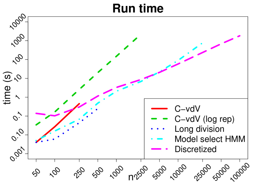
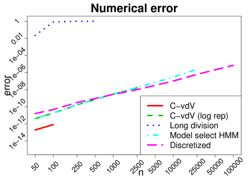
Figure 2: Run time and numerical accuracy for the exact algorithms from Section 2 in calculating $q_{n,i}$ for $i=1,\ldots,n$. A numerical error of $10^{-a}$ means that the algorithm is able to calculate the mathematically exact answer up to $a$ decimal places.

In this section we investigate the speed and numerical accuracy of our new algorithms to the previously proposed methods for exact computation of the posterior. We consider a sequence of sample sizes $n=50,\allowbreak 100,\allowbreak 250,\allowbreak 500,\allowbreak 1\,000,\allowbreak 2\,500,\allowbreak...,\allowbreak 50\,000,\allowbreak 100\,000$ and construct the true signal $\theta_{0}$ to have $20\%$ non-zero signal components of value $4\sqrt{2\ln n}$, while the rest of the signal coefficients are set to be zero. For fair comparison we run all algorithms for the spike-and-slab prior with Laplace slab $g(x)=\frac{a}{2}e^{-a|x|}$, with $a=1$, and mixing hyper-prior $\Lambda_{n}=\operatorname{Beta}(1,n+1)$. We have set up the experiments in R, but all algorithms were implemented as subroutines in C++. Since numerical instability is a major concern, we have tracked the numerical accuracy of all methods using interval arithmetic as implemented in the C++ Boost library [8] (with cr-libm as a back-end to compute transcendental functions [21]), which replaces all floating point numbers by intervals that are guaranteed to contain the mathematically exact answer. The lower end-point of each interval corresponds to always rounding down in the calculations, and the upper end-point corresponds to always rounding up. The width of the interval for the final answer therefore measures the numerical error. All experiments were performed on a MacBook Pro laptop with 2.9 GHz Intel Core i5 processor, 8 GB (1867 MHz DDR3) memory, and a solid-state hard drive.

Results

The results are summarized in Figure 2, which shows the run time of the algorithms on the left, and their numerical error on the right. The reported numerical error is the maximum numerical error in calculating $q_{n,i}$ over $i=1,\ldots,n$. To avoid overly long computations we have terminated the algorithms if they became numerically unstable or if their run time exceeded half an hour. One can see that the original Castillo-Van der Vaart algorithm was terminated for $n\geq 250$, which was due to numerical inaccuracy. This problem was resolved by applying the logarithmic representation from Appendix A.2 which made the algorithm numerically stable up to $n\leq 2500$; however, due to the long $O(n^{3})$ run time the algorithm was terminated for larger values as it reached the half-hour limit. The natural speed-up idea of applying long division (see Appendix A.3) was not successful for this data as even for small sample sizes the numerical accuracy was poor. We observe that the model selection HMM and the algorithm based on discretization performed superior to the preceding methods: the model selection HMM algorithm has run time $O(n^{2})$ and the largest sample size it managed to complete within half an hour was $n=25\,000$, while the algorithm with discretized mixing parameter in the spike-and-slab prior (initialized according to Corollary 2.2 with parameter $m=20$) has run time $O(n^{3/2})$ and reached the time limit after sample size $n=100\,000$. We also note that both algorithms were numerically accurate, giving answers that were reliable up to between 5 and 11 decimal places, depending on $n$. For sample size $n=2\,500$, we have further verified empirically that indeed the model selection HMM algorithm computes the same numbers as the Castillo-Van der Vaart algorithm, as was already shown in Section 2.1.

3.2 Approximation Errors for Several Standard Methods

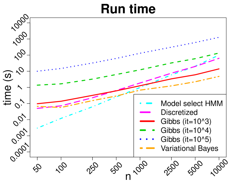
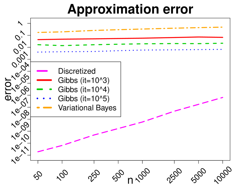
Figure 3: Run times and approximation errors for approximate algorithms. An approximation error of $10^{-a}$ means that the algorithm is able to calculate the correct answer up to $a$ decimal places.

Table 1: Approximation errors compared to the exact HMM algorithm

Method \ n	100	250	500	1 000	2 500	5 000	10 000
Discretized	$\mathbf{6.37\times 10^{-11}}$	$\mathbf{4.89\times 10^{-10}}$	$\mathbf{1.67\times 10^{-9}}$	$\mathbf{5.89\times 10^{-9}}$	$\mathbf{4.69\times 10^{-8}}$	$\mathbf{1.74\times 10^{-7}}$	$\mathbf{6.56\times 10^{-7}}$
Gibbs ($\text{it}=10^{3}$)	$4.58\times 10^{-2}$	$4.76\times 10^{-2}$	$5.03\times 10^{-2}$	$5.41\times 10^{-2}$	$6.15\times 10^{-2}$	$6.28\times 10^{-2}$	$6.96\times 10^{-2}$
Gibbs ($\text{it}=10^{4}$)	$1.23\times 10^{-2}$	$1.46\times 10^{-2}$	$1.63\times 10^{-2}$	$1.75\times 10^{-2}$	$2.03\times 10^{-2}$	$2.07\times 10^{-2}$	$2.25\times 10^{-2}$
Gibbs ($\text{it}=10^{5}$)	$4.55\times 10^{-3}$	$5.05\times 10^{-3}$	$5.46\times 10^{-3}$	$5.63\times 10^{-3}$	$5.71\times 10^{-3}$	$6.86\times 10^{-3}$	$6.88\times 10^{-3}$
Variational Bayes	$1.90\times 10^{-1}$	$2.48\times 10^{-1}$	$2.93\times 10^{-1}$	$3.33\times 10^{-1}$	$3.91\times 10^{-1}$	$4.40\times 10^{-1}$	$4.81\times 10^{-1}$

In this section we measure the approximation error of a selection of approximation algorithms by comparing them to the exact model selection HMM algorithm, which serves as a benchmark for the correct answer. We again consider the spike-and-slab prior with $\Lambda_{n}=\operatorname{Beta}(1,n+1)$, but for simplicity we use standard Gaussian slabs $g(x)=\frac{1}{\sqrt{2\pi}}e^{-x^{2}}$, since the approximation methods are typically designed for this choice of slab distribution. Our first approximation method is the discretization algorithm from Section 2.2.1, which uses a deterministic approximation. The discretization algorithm was again initialized according to Corollary 2.2 with $m=20$. We further consider a standard Gibbs sampler (with number of iterations $\text{it}=10^{3},10^{4},10^{5}$, half of which are used as burn-in) and a variational Bayes approximation. We consider the same test data as in the preceding section. The only difference is that we stop at $n=10\,000$ to limit the run times for the exact HMM algorithm and the Gibbs sampler with $\text{it=}10^{5}$. Both the Gibbs sampler and variational Bayes algorithm were implemented in R. For the latter we used the component-wise variational Bayes algorithm [38, 57, 10, 47]. We measure approximation error by computing $\max_{i}|q_{n,i}-\tilde{q}_{n,i}|$, where $q_{n,i}$ is the exact slab probability computed by the model selection HMM and $\tilde{q}_{n,i}$ is the slab probability computed by the approximation. We run each non-deterministic approximation method 5 times and report the average approximation error along with the average run time of the algorithms. The results are plotted in Figure 3 and shown numerically in Table 1.

One can see that the discretized version of the algorithm is very accurate, with at least seven decimal places of precision throughout. It approximately loses two decimal places of precision for every ten-fold increase of $n$, so we can still expect it to be accurate up to five decimal places for $n=100\,000$. We point out that its approximation error includes both the mathematical approximation from Section 2.2.1 and the numerical error already studied separately in Figure 2. Since the approximation error in Figure 3 is of the same order as the numerical error in Figure 2, we conclude that the numerical error dominates the mathematical approximation error, so the discretization algorithm may be considered an exact method for all practical purposes.

At the same time the Gibbs sampler and the variational Bayes method both provide approximations of the posterior that are far less accurate. Variational Bayes is only accurate up to one decimal place, although in further investigations we did find that it provides a better approximation if we look only at the non-zero coefficients, with an approximation error of order $O(10^{-4})$. For the Gibbs sampler there is no theory that tells us how many iterations we have to take to achieve a certain degree of accuracy. We see here that the precision strongly depends on the number of iterations, ranging from one to three decimal places, but remains approximately constant with increasing $n$. However, the run time for $\text{it}=10^{5}$ iterations would become prohibitive for sample sizes much larger than the $n=10\,000$ we consider.

4 Differential Gene Expression for Ulcerative Colitis and Crohn’s Disease

In this section we compare our methods to various other frequently used Bayesian approaches in the context of differential gene expression data.

Data

We consider a data set from Burczynski et al. [9] containing the gene expression levels of $n=22\,283$ genes in peripheral blood mononuclear cells, with the raw data provided by the National Center for Biotechnology Information. This is an observational study, with microarray gene expression data on 26 subjects who suffered from ulcerative colitis and 59 subjects with Crohn’s disease. We calculate Z-scores to identify differences in average gene expression levels between the two disease groups following the standard approach described by Quackenbush [45], which consists of dividing the difference of the average log-transformed, normalized gene expressions for the two groups by the standard error. More specifically, let us denote by $U_{i,j}$ and $C_{i,j}$ the measured intensities of the $i$-th gene and $j$-th person with ulcerative colitis and Crohn’s disease, respectively. As a first step we normalize the intensities for each patient, i.e. we take $U_{i,j}^{\prime}=U_{i,j}/\sum_{i}U_{i,j}$ and $C_{i,j}^{\prime}=C_{i,j}/\sum_{i}C_{i,j}$ for each gene $i$ and patient $j$. Then the Z-score for the $i$-th gene is computed as

$$Z_{i}=\frac{\overline{\log U_{i}^{\prime}}-\overline{\log C_{i}^{\prime}}}{\sqrt{\sigma^{2}_{U^{\prime},i}/26+\sigma^{2}_{C^{\prime},i}/59}}\qquad\text{for $i=1,\ldots,22\,283$,}$$

where

$$\overline{\log U_{i}^{\prime}}=\frac{1}{26}\sum_{j=1}^{26}\log U_{i,j}^{\prime},\quad\sigma^{2}_{U^{\prime},i}=\frac{1}{25}\sum_{j=1}^{26}\big{(}\log U_{i,j}^{\prime}-\overline{\log U_{i}^{\prime}}\big{)}^{2},$$

and $\overline{\log C_{i}^{\prime}}$ and $\sigma^{2}_{C^{\prime},i}$ are defined accordingly. Since it is assumed that the number of genes with a different expression level between the two groups is small compared to the total number of genes $n$, the data fit into the sparse normal sequence model with $n=22\,283$.

Methods

Table 2: Run time and number of selected genes on gene expression data. The reported run times for Empirical Bayes EBSparse and the Horseshoe are the averages over their runs.

Method	Run Time	Nr. of Genes Selected
Variational Bayes (varbvs)	20.95 minutes	166
Spike-and-Slab LASSO	0.01 seconds	557
Horseshoe (10 runs)	1.86 minutes	571–583
Empirical Bayes EBSparse (10 runs)	7.28 seconds	592–604
Discretized: $\operatorname{Beta}(1,n+1)$-binomial prior	24.47 seconds	674
HMM: $\operatorname{Beta}(1,n+1)$-binomial prior	2.06 minutes	674
Empirical Bayes JS	0.03 seconds	3168
HMM: $\operatorname{Beta}(1,1)$-binomial prior	2.00 minutes	3169

We compare the run times and the selected genes for the eight procedures listed in Table 2. We consider the model selection HMM algorithm for the $\operatorname{Beta}(1,n+1)$-binomial prior with Laplace slab (with hyper-parameter $a=0.5$), and the discretization algorithm from Corollary 2.2 with $m=20$, which is a faster way to compute exactly the same results. Genes $i$ with marginal posterior probability $q_{n,i}\geq 1/2$ are selected. For comparison, we also consider the model selection HMM for the $\operatorname{Beta}(1,1)$-binomial prior, which corresponds to using a uniform prior $\Lambda_{n}$ on the mixing parameter $\alpha$. In this section, we used the implementations of our algorithms from our R package [62], which is approximately 5 times faster than the implementation from Section 3, because it does not incur the overhead of tracking numerical accuracy using interval arithmetic.

We compare to the empirical Bayes method of Johnstone and Silverman [31], which uses a spike-and-slab prior, but estimates the mixing parameter $\alpha$ using empirical Bayes. The method does not explicitly include a prior on $\alpha$, but we may interpret it as using a uniform prior $\Lambda_{n}$. We again use a Laplace slab (with the default parameter $a=0.5$) and select genes by hard thresholding at marginal posterior probability $1/2$, as implemented in the R package [55].

We also include EBSparse, which is a fractional empirical Bayes procedure proposed by Martin and Walker [40]. It can be interpreted as using a spike-and-slab prior with $\Lambda_{n}=\operatorname{Beta}(1,\gamma n)$, but with Gaussian slabs $G_{i}=\operatorname{\mathcal{N}}(Y_{i},\tau^{2})$ whose means depend on the data. Furthermore, in the formula for the posterior the likelihood is tempered by raising it to the power $\kappa$. We use the authors’ R implementation [41], with the recommended hyper-parameter settings $\kappa=0.99$, $\gamma=0.25$, $\tau^{2}=100$, and $M=1000$ Monte Carlo samples. As the sampler is randomized, we run the algorithm $10$ times.

We further consider the Spike-and-Slab LASSO of Ročková [48], which computes the maximum a posteriori parameters using Laplace distributions both for the spikes and for the slabs. As in [48, Section 6], we take the slab scale parameter to be $\lambda_{1}=0.1$, and estimate the spike scale parameter $\lambda_{0}$ via the two-step procedure described there, for the $\operatorname{Beta}(1,n+1)$ hyper-prior on the mixing parameter. An R implementation called SSLasso was provided by Ročková [49].

We also add the Horseshoe estimator [11] with the Cauchy hyper-prior on its hyper-parameter $\tau$, truncated to the interval $[1/n,1]$, as recommended by Van der Pas et al. [59]. We use the R package [58], with its default Markov Chain Monte Carlo sampler settings of $1000$ iterations burn-in and $5000$ iterations after burn-in. Genes are selected if their credible sets exclude zero [59]. As the sampler is randomized, we run the algorithm $10$ times.

Finally, we compare with the variational Bayes algorithm (varbvs R-package) described in [10]. Notably, this method uses Gaussian slabs. The hyper-parameters (e.g. the variance of the prior and the noise) are automatically fitted to the data. We set the tolerance and maximum number of iterations to be $10^{-4}$ and $1000$, respectively.

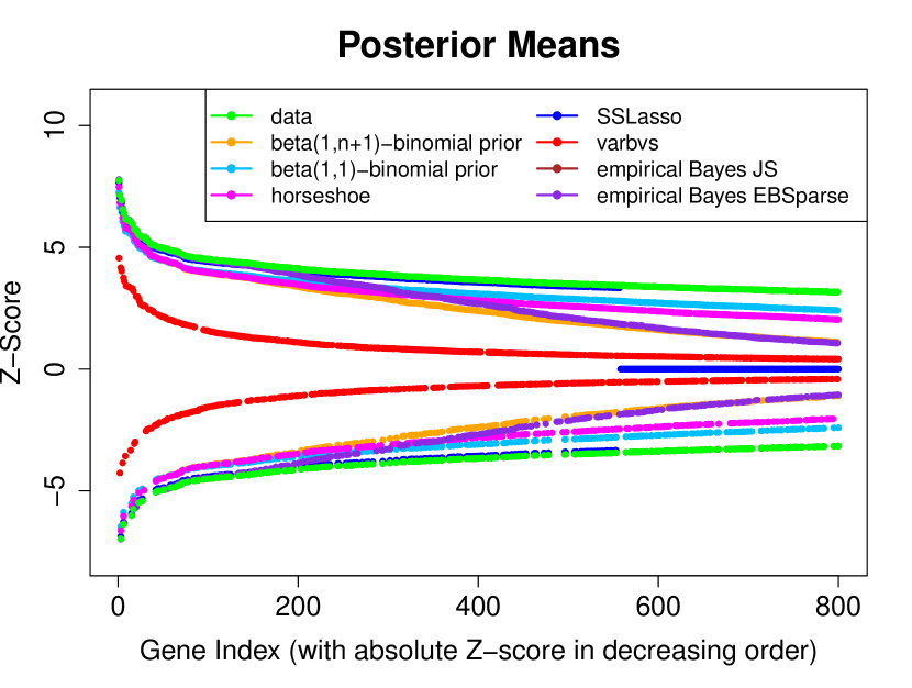
Figure 4: Posterior means/MAP estimates for the $800$ genes in the gene expression data with largest Z-scores (in absolute value)

Results

Results are reported in Table 2 and Figure 4. Although we list run times to illustrate computational feasibility, it is important to keep in mind that the methods in this section compute different quantities, so their most important difference lies in which genes they select. On this point, the main conclusion is that the alternative methods give very different results from using the exact Bayesian posterior for the model selection prior.

All methods except the Horseshoe and EBSparse select genes in decreasing order of the absolute values of $Z_{i}$. Genes are generally selected by the Horseshoe and EBSparse in decreasing order of absolute value of $Z_{i}$ as well, but with some swaps for genes for which the absolute values are close to each other, so it appears that for all sampling-based methods the sampler is suffering from limited precision, as we also observed for the Gibbs samplers in Section 3.2. The methods can be divided into three main categories based on the number of genes they select: on one extreme is the variational Bayes (varbvs) method, which provides the sparsest solution; then the majority of methods select a number of genes between $557$ and $674$; and finally at the other extreme are the Empirical Bayes JS procedure and the $\operatorname{Beta}(1,1)$-binomial prior, which are both based on the same prior and both select a very large number of genes, making these two methods the most conservative. The lack of sparsity induced by the $\operatorname{Beta}(1,1)$-binomial prior is perhaps not surprising, given that it does not satisfy the exponential decrease condition of [16]. We study this further in Section 5, where we compare different choices for the hyper-parameters of the beta-binomial prior in simulations.

We further see that the Spike-and-Slab LASSO and the empirical Bayes JS procedures finish almost instantly. The EBSparse method takes several seconds to run, as does the discretization algorithm. The Horseshoe and our exact model selection HMM take approximately two minutes to run, while the variational Bayes varbvs method requires a little over 20 minutes. Nevertheless, all methods are feasible even for practitioners who would like to perform multiple similar experiments, for example with different variations of the prior or slab distributions. By contrast, we do not include the Castillo-Van der Vaart algorithm with logarithmic representation, because based on extrapolation of Figure 2 we expect it to take around 20 days.

In Figure 4 we also plot the posterior means (or, in case of the Spike-and-Slab LASSO, the MAP estimator) and the $800$ largest Z-scores in absolute value. Since the posterior means for the model selection HMM and the discretization algorithm are the same, we label both as $\operatorname{Beta}(1,n+1)$-binomial in reference to the prior that was used. We further note that the empirical Bayes JS estimates are invisible behind the data points. We observe that the varbvs method induces the heaviest shrinkage, followed first by the $\operatorname{Beta}(1,n+1)$-binomial prior and the Empirical Bayes EBSparse method, and then by the Horseshoe and the $\operatorname{Beta}(1,1)$-binomial prior. The least shrinkage is applied by the empirical Bayes JS method, which does not shrink the observed Z-scores very much (if at all). The Spike-and-Slab LASSO is in a category of its own, because it is a MAP estimator. It applies no shrinkage to the coefficients that are selected, and sets all other coefficients to zero.

5 Asymptotics of Spike-and-Slab Priors

The choice of the prior $\Lambda_{n}$ on the mixing hyper-parameter $\alpha$ in spike-and-slab priors is considered to be highly relevant for the behavior of the posterior. Castillo and Van der Vaart [16] recommend to use $\Lambda_{n}=\operatorname{Beta}(\kappa,\lambda)$ with parameters $\kappa=1$ and $\lambda=n+1$. This prior induces heavy penalization for dense models (models with large sparsity parameter $s$) and was shown to have optimal theoretical properties. However, it is unknown whether such heavy penalization is indeed necessary and whether even heavier penalization will result in suboptimal behavior.

In this section we investigate the asymptotic behavior of the posterior for different choices of the hyper-parameters $\kappa$ and $\lambda$ using our new exact algorithms, which can scale up to large sample sizes. We consider: i) the uniform prior with $\kappa=1$ and $\lambda=1$, which is often considered a natural choice [54]; ii) mild shrinkage, $\kappa=1$ and $\lambda=\sqrt{n}$; iii) the choice $\kappa=1$ and $\lambda=n+1$ recommended by Castillo and Van der Vaart; iv) heavy shrinkage, $\kappa=1$ and $\lambda=n^{2}$ ; and finally v) a sparsity-discouraging choice, $\kappa=n$ and $\lambda=1$. We consider two experiments: $A_{1}$ and $A_{2}$. In both cases the sample sizes range from $n=50$ to $n=20\,000$. In Experiment $A_{1}$ we set the true sparsity level to $s=10$ and consider uniformly distributed non-zero signal coefficients between 1 and 10, i.e. $\theta_{i}\sim U(1,10)$ for $i\in\mathcal{S}$. In Experiment $A_{2}$ the true sparsity level is taken to be $s=\lceil n^{1/3}\rceil$ and the non-zero signal coefficients are set to $\theta_{i}=2\sqrt{2\log n}$ for $i\in\mathcal{S}$, which is a factor of $2$ above the detection threshold. In Appendix B of the supplementary material we consider an additional experiment $A_{3}$ that is similar to $A_{1}$ but with $s=25$ and $\theta_{i}\sim U(5,10)$ for $i\in\mathcal{S}$, which gives similar results as Experiment $A_{1}$.

Table 3: $\ell_{2}$ distance of the posterior mean from the true signal in Experiment $A_{1}$

Method \ n	50	100	200	500	1 000	2 000	5 000	10 000	20 000
i) $\kappa=1$, $\lambda=1$	4.52 (0.64)	4.65 (0.68)	4.84 (0.75)	5.30 (1.01)	5.18 (0.74)	5.63 (0.90)	5.95 (0.77)	6.65 (1.26)	6.38 (0.98)
ii) $\kappa=1$, $\lambda=\sqrt{n}$	4.28 (0.63)	4.46 (0.69)	4.69 (0.75)	5.20 (1.01)	5.13 (0.73)	5.57 (0.88)	5.92 (0.78)	6.62 (1.27)	6.36 (0.98)
iii) $\kappa=1$, $\lambda=n+1$	4.09 (0.68)	4.20 (0.82)	4.43 (0.88)	4.95 (1.11)	5.14 (0.89)	5.45 (0.99)	6.18 (0.94)	6.42 (1.67)	6.43 (1.06)
iv) $\kappa=1$, $\lambda=n^{2}$	5.04 (1.05)	5.21 (1.42)	6.55 (1.48)	7.09 (1.93)	7.87 (1.21)	8.15 (1.42)	9.45 (1.55)	10.35 (2.24)	10.43 (2.16)
v) $\kappa=n$, $\lambda=1$	5.71 (0.59)	7.60 (0.62)	10.63 (0.54)	16.89 (0.61)	23.39 (0.61)	33.43 (0.78)	52.93 (0.52)	74.79 (0.57)	105.84 (0.55)

Table 4: False discovery rate in Experiment $A_{1}$

Method \ n	50	100	200	500	1 000	2 000	5 000	10 000	20 000
i) $\kappa=1$, $\lambda=1$	0.36 (0.14)	0.23 (0.13)	0.19 (0.11)	0.13 (0.12)	0.05 (0.09)	0.09 (0.12)	0.08 (0.09)	0.12 (0.10)	0.08 (0.09)
ii) $\kappa=1$, $\lambda=\sqrt{n}$	0.16 (0.10)	0.16 (0.11)	0.17 (0.11)	0.11 (0.11)	0.06 (0.09)	0.09 (0.12)	0.08 (0.08)	0.11 (0.10)	0.08 (0.09)
iii) $\kappa=1$, $\lambda=n+1$	0.05 (0.06)	0.03 (0.05)	0.02 (0.04)	0.02 (0.04)	0.01 (0.03)	0.01 (0.02)	0.00 (0.00)	0.01 (0.03)	0.00 (0.00)
iv) $\kappa=1$, $\lambda=n^{2}$	0.00 (0.00)	0.00 (0.00)	0.00 (0.00)	0.00 (0.00)	0.00 (0.00)	0.00 (0.00)	0.00 (0.00)	0.00 (0.00)	0.00 (0.00)
v) $\kappa=n$, $\lambda=1$	0.80 (0.00)	0.90 (0.00)	0.95 (0.00)	0.98 (0.00)	0.99 (0.00)	1.00 (0.00)	1.00 (0.00)	1.00 (0.00)	1.00 (0.00)

Table 5: True positive rate in Experiment $A_{1}$

Method \ n	50	100	200	500	1 000	2 000	5 000	10 000	20 000
i) $\kappa=1$, $\lambda=1$	0.91 (0.11)	0.83 (0.15)	0.86 (0.08)	0.80 (0.17)	0.76 (0.13)	0.73 (0.17)	0.73 (0.13)	0.71 (0.14)	0.66 (0.16)
ii) $\kappa=1$, $\lambda=\sqrt{n}$	0.89 (0.11)	0.83 (0.14)	0.85 (0.09)	0.78 (0.17)	0.75 (0.13)	0.73 (0.17)	0.72 (0.13)	0.71 (0.15)	0.65 (0.16)
iii) $\kappa=1$, $\lambda=n+1$	0.84 (0.12)	0.76 (0.11)	0.80 (0.10)	0.74 (0.18)	0.70 (0.12)	0.68 (0.18)	0.64 (0.12)	0.64 (0.19)	0.59 (0.15)
iv) $\kappa=1$, $\lambda=n^{2}$	0.71 (0.14)	0.62 (0.14)	0.59 (0.16)	0.57 (0.17)	0.52 (0.13)	0.48 (0.20)	0.44 (0.15)	0.40 (0.17)	0.38 (0.16)
v) $\kappa=n$, $\lambda=1$	1.00 (0.00)	1.00 (0.00)	1.00 (0.00)	1.00 (0.00)	1.00 (0.00)	1.00 (0.00)	1.00 (0.00)	1.00 (0.00)	1.00 (0.00)

We repeat each experiment 20 times and report the average $\ell_{2}$-error between the posterior mean for $\theta$ and the true signal $\theta$ in Table 3 and Table 6 for Experiments $A_{1}$ and $A_{2}$, respectively. In Tables 4, 5, 7 and 8 we also report the average false discovery rates and the average true positive rates. Standard deviations are provided in parentheses in all cases.

Table 6: $\ell_{2}$ distance of the posterior mean from the true signal in Experiment $A_{2}$

Method \ n	50	100	200	500	1 000	2 000	5 000	10 000	20 000
i) $\kappa=1$, $\lambda=1$	3.03 (0.98)	3.77 (0.70)	3.9 (0.58)	4.48 (0.96)	4.68 (0.51)	5.65 (0.84)	7.13 (0.81)	7.70 (1.21)	8.68 (0.82)
ii) $\kappa=1$, $\lambda=\sqrt{n}$	2.79 (0.91)	3.56 (0.68)	3.80 (0.59)	4.32 (0.93)	4.55 (0.51)	5.53 (0.83)	7.02 (0.81)	7.61 (2.15)	8.59 (1.21)
iii) $\kappa=1$, $\lambda=n+1$	2.41 (0.88)	3.01 (0.68)	3.07 (0.74)	3.48 (0.79)	3.64 (0.62)	4.27 (0.63)	5.33 (0.78)	5.68 (0.94)	6.32 (0.77)
iv) $\kappa=1$, $\lambda=n^{2}$	3.43 (1.82)	3.63 (2.06)	3.89 (1.86)	5.13 (2.51)	4.49 (1.90)	5.08 (2.27)	5.62 (1.42)	6.27 (2.15)	6.42 (1.70)
v) $\kappa=n$, $\lambda=1$	5.31 (0.84)	7.69 (0.48)	10.67 (0.52)	16.81 (0.71)	23.56 (0.56)	33.59 (0.50)	53.00 (0.44	74.92 (0.53)	105.8 (0.54)

Table 7: False discovery rate in Experiment $A_{2}$

Method \ n	50	100	200	500	1 000	2 000	5 000	10 000	20 000
i) $\kappa=1$, $\lambda=1$	0.25 (0.22)	0.22 (0.17)	0.15 (0.12)	0.12 (0.09)	0.10 (0.08)	0.11 (0.08)	0.11 (0.06)	0.12 (0.06)	0.10 (0.03)
ii) $\kappa=1$, $\lambda=\sqrt{n}$	0.15 (0.16)	0.18 (0.14)	0.14 (0.11)	0.11 (0.09)	0.08 (0.08)	0.10 (0.08)	0.10 (0.06)	0.11 (0.06)	0.10 (0.03)
iii) $\kappa=1$, $\lambda=n+1$	0.01 (0.04)	0.06 (0.08)	0.03 (0.07)	0.04 (0.06)	0.01 (0.03)	0.02 (0.05)	0.02 (0.03)	0.02 (0.02)	0.01 (0.02)
iv) $\kappa=1$, $\lambda=n^{2}$	0.00 (0.00)	0.00 (0.00)	0.00 (0.00)	0.00 (0.00)	0.00 (0.00)	0.00 (0.00)	0.00 (0.00)	0.00 (0.00)	0.00 (0.00)
v) $\kappa=n$, $\lambda=1$	0.92 (0.00)	0.95 (0.00)	0.97 (0.00)	0.98 (0.00)	0.99 (0.00)	0.99 (0.00)	1.00 (0.00)	1.00 (0.00)	1.00 (0.00)

Table 8: True positive rate in Experiment $A_{2}$

Method \ n	50	100	200	500	1 000	2 000	5 000	10 000	20 000
i) $\kappa=1$, $\lambda=1$	1.00 (0.00)	1.00 (0.00)	1.00 (0.00)	1.00 (0.00)	1.00 (0.00)	1.00 (0.00)	1.00 (0.00)	1.00 (0.00)	1.00 (0.00)
ii) $\kappa=1$, $\lambda=\sqrt{n}$	1.00 (0.00)	1.00 (0.00)	1.00 (0.00)	1.00 (0.00)	1.00 (0.00)	1.00 (0.00)	1.00 (0.00)	1.00 (0.00)	1.00 (0.00)
iii) $\kappa=1$, $\lambda=n+1$	1.00 (0.00)	1.00 (0.00)	1.00 (0.00)	1.00 (0.00)	1.00 (0.00)	1.00 (0.00)	1.00 (0.00)	1.00 (0.00)	1.00 (0.00)
iv) $\kappa=1$, $\lambda=n^{2}$	0.89 (0.19)	0.94 (0.09)	0.94 (0.08)	0.95 (0.09)	0.98 (0.05)	0.99 (0.03)	0.99 (0.02)	0.99 (0.02)	1.00 (0.01)
v) $\kappa=n$, $\lambda=1$	1.00 (0.00)	1.00 (0.00)	1.00 (0.00)	1.00 (0.00)	1.00 (0.00)	1.00 (0.0v0)	1.00 (0.00)	1.00 (0.00)	1.00 (0.00)

In Experiment $A_{1}$ we see that the $\ell_{2}$-error is not very sensitive to the choice of hyperparameters: the uniform prior i), the mild shrinkage ii), and Castillo and Van der Vaart’s recommendation iii) all perform comparably. Only the heavy shrinkage iv) is introducing too high penalization, especially for large models. Unsurprisingly, the choice of hyper-parameters v) is also substantially worse than the others, because it expresses exactly the wrong type of prior assumptions by heavily penalizing sparse models. In Experiment $A_{2}$ we see that the best hyper-parameters are Castillo and Van der Vaart’s recommendation iii) and the heavy shrinkage iv), with the latter having a large variability in performance. Hyper-parameter choices i) and ii) are introducing no or only mild penalization for large models and indeed are also observed to have somewhat worse performance than choices iii) and iv), with the difference getting more pronounced for larger sample sizes. Finally, as in Experiment $A_{1}$, the hyper-parameter setting v) is the worst by far.

We also study the false discovery rate (FDR) and true positive rate (TPR) of the spike-and-slab priors (relatedly, see [14] for the theoretical underpinning of FDR control with empirical Bayes spike-and-slab priors). Unsurprisingly, the FDR is smallest in both experiments in case of heavy shrinkage v), but almost equally good rates are obtained for the recommended choice iii). Mild ii) or no i) shrinkage result in somewhat worse FDR, while the sparsity discouraging setting v) essentially selects all the noise. In Experiment $A_{1}$ the best TPR is obtained, not surprisingly, by setting v), which conservatively selects everything. Hyper-parameter choices i) and ii) perform comparably well, closely followed by iii), while the heavy shrinkage method iv) is substantially worse. In Experiment $A_{2}$ all hyper-parameter settings perform equally well, except for the heavy shrinkage iv), which is slightly worse. The good performance of the methods is due to the relatively high value ($2\sqrt{2\log n}$) for the non-zero signal coefficients, which lies above the detection threshold $\sqrt{2\log n}$.

We conclude that, overall, the recommended choice iii) indeed appears to have an advantage over the alternatives, and that even heavier penalization as in choice iv) is harmful.

The above simulation study is just one example of how our exact algorithms can be used to study asymptotic properties of model selection priors, and more specifically spike-and-slab priors. Another possible application not considered here would, for instance, be to study the accuracy of Bayesian uncertainty quantification (see [15] for frequentist coverage of Bayesian credible sets resulting from empirical Bayes spike-and-slab priors).

6 Discussion

We have proposed fast and exact algorithms for computing the Bayesian posterior distribution corresponding to model selection priors (including spike-and-slab priors as a special case) in the sparse normal sequence model. Since the normal sequence model corresponds to linear regression with identity design, the question arises whether the derived algorithms can be extended to sparse linear regression with more general designs or other more complex models. We first note that all methods are agnostic about where the conditional densities of the spikes $p(Y_{i}\mid B_{i}=0)=\phi(Y_{i})$ and the slabs $p(Y_{i}\mid B_{i}=1)=\psi(Y_{i})$ come from. It is therefore trivial to extend them to any model that replaces the distribution of $Y_{i}$ given $\mathcal{S}$ by

$$Y_{i}\mid\mathcal{S}\sim\begin{cases}\psi_{i}&\text{if $i\in\mathcal{S}$,}\\ \phi_{i}&\text{otherwise,}\end{cases}$$

for any densities $\psi_{i}$ and $\phi_{i}$. (In fact, this is already supported by our R package [62].) Such extensions make it possible to easily handle other noise models for $\varepsilon_{i}$ or general diagonal designs; and, as pointed out by a referee, it also allows incorporating a non-atomic prior on $\theta_{i}$ in case $i\not\in\mathcal{S}$. We further anticipate that extensions to general sparse design matrices may be possible by generalizing the HMM from Section 2.1 to more general Bayesian networks and applying a corresponding inference algorithm to compute marginal posterior probabilities. However, for non-sparse design matrices the extension would be very challenging, if possible at all, because the Bayesian network of the hidden states could become fully connected. An interesting intermediate case is studied by Papaspiliopoulos and Rossell [43], who consider best-subset selection for block-diagonal designs. For the normal sequence model, their assumptions amount to the requirement that $\Lambda_{n}$ is a point-mass on a single $\alpha$, and they point out that in this case “best-subset selection becomes trivial.” For non-diagonal designs their results are non-trivial, because they are able to integrate over a continuous hyper-prior on the variance $\sigma^{2}$ of the noise $\varepsilon_{i}$. In contrast, we assume fixed $\sigma^{2}$, which we then take to be $\sigma^{2}=1$ without loss of generality. Our methods can be used to calculate the marginal likelihood $p(Y\mid\sigma^{2})$ without further computational overhead, so it would be possible to run them multiple times to incorporate a discrete prior on a grid of values for $\sigma^{2}$, but it is not obvious if our results can be extended to continuous priors over $\sigma^{2}$. Exploration of these directions is left for future work.

Even without extending our methods to full linear regression or continuous priors on $\sigma^{2}$, we believe that they are already very useful as a benchmark procedure: any approximation technique for general linear regression may be applied to the special case of sparse normal sequences and its approximation error computed as in Section 3.2. If a method does not work well in this special case, then certainly we cannot trust it for more general regression. The existence of such a benchmark method is very important, since, for instance, there are no available diagnostics to determine whether Markov Chain Monte Carlo samplers have converged to their stationary distribution or if they have explored a sufficient proportion of the models in the model space.

We have also explored the exact connection between general model selection priors and the more specific spike-and-slab priors. Since for spike-and-slab priors one can construct faster algorithms, it is useful to know which model selection priors can be represented in this form. The proof of our result amounts to a finite sample version of de Finetti’s theorem for a particular subclass of exchangeable distributions, which may be of interest in its own right.

Supplementary Material

The supplement contains a review of the exact algorithm by Castillo and Van der Vaart and a discussion on how to perform all computations in a logarithmic representation. It further includes an additional variation on Experiment $A_{1}$ from Section 5. Finally, the proofs for all theorems and the examples from Section 2.3 are also given in the supplement.

Supplementary Material

Appendix A The Castillo-Van der Vaart Algorithm

In this section we first recall the Castillo-Van der Vaart algorithm [16]. Straight-forward implementation of the algorithm fails for sample sizes larger than $n\geq 500$, because the intermediate results exceed the maximum range that can be numerically represented. Fortunately, this can be resolved by performing all computations in a logarithmic representation, which we discuss second. The bottleneck then becomes the algorithm’s computational complexity, because it requires $O(n^{3})$ steps, which is prohibitive for large $n$. At the end of this appendix we discuss two possible speed ups of the algorithm based on fast polynomial multiplication and long division, respectively, and show that neither of them works well practice.

A.1 Description of the algorithm

The key ingredient of the Castillo-Van der Vaart algorithm is their observation that, for any $s\in\{0,1,\ldots,n\}$ and any sequences of numbers $a=(a_{1},\ldots,a_{n})$ and $b=(b_{1},\ldots,b_{n})$, the sum

$$C_{s}(a,b)=\sum_{|\mathcal{S}|=s}\prod_{i\in\mathcal{S}}a_{i}\prod_{i\neq\mathcal{S}}b_{i}$$

is the coefficient of $Z^{s}$ in the polynomial

$$Z\mapsto\prod_{i=1}^{n}(a_{i}Z+b_{i}).$$ (9)

All coefficients of this polynomial can be computed in $O(n^{2})$ operations by computing the products term by term, which is much faster than explicitly summing over the exponentially many subsets of size $s$. This observation allows Castillo and Van der Vaart to compute the Bayesian marginal likelihood as follows:

$$Q_{n}=\sum_{s=0}^{n}\frac{\pi_{n}(s)}{\binom{n}{s}}\sum_{|\mathcal{S}|=s}\prod_{i\in\mathcal{S}}\psi(Y_{i})\prod_{i\neq\mathcal{S}}\phi(Y_{i})=\sum_{s=0}^{n}\frac{\pi_{n}(s)}{\binom{n}{s}}C_{s}(\Psi,\Phi),$$ (10)

with $\Psi=(\psi(Y_{1}),\ldots,\psi(Y_{n}))$ and $\Phi=(\phi(Y_{1}),\ldots,\phi(Y_{n}))$.  The binomial coefficients can be precomputed in $O(n)$ time using the recursion $\binom{n}{s}=\binom{n}{s-1}(n-s+1)/s$. Assuming that $\pi_{n}(s)$ can be evaluated efficiently, computing the sum in (10) then takes another $O(n)$ steps, which means that the computation of the coefficients $C_{s}(\Psi,\Phi)$ is the dominant factor and all together $Q_{n}$ can be computed in $O(n^{2})$ steps.

The same idea can be used again to compute the marginal posterior probabilities

$$q_{n,i} =\frac{1}{Q_{n}}\sum_{s=1}^{n}\frac{\pi_{n}(s)}{\binom{n}{s}}\psi(Y_{i})\sum_{\begin{subarray}{c}|\mathcal{S}|=s\\ i\in\mathcal{S}\end{subarray}}\prod_{\begin{subarray}{c}j\in\mathcal{S}\\ j\neq i\end{subarray}}\psi(Y_{j})\prod_{j\neq\mathcal{S}}\phi(Y_{j})$$

$$=\frac{1}{Q_{n}}\sum_{s=1}^{n}\frac{\pi_{n}(s)}{\binom{n}{s}}\sum_{|\mathcal{S}|=s}\prod_{j\in\mathcal{S}}\Psi_{j}\prod_{j\neq\mathcal{S}}\Phi^{i}_{j}=\frac{1}{Q_{n}}\sum_{s=1}^{n}\frac{\pi_{n}(s)}{\binom{n}{s}}C_{s}(\Psi,\Phi^{i}),$$ (11)

where $\Psi$ is as before, and $\Phi^{i}$ equals $\Phi$ except that the $i$-th component is replaced by $0$. When $Q_{n}$ has been precomputed, calculating $q_{n,i}$ takes $O(n^{2})$ operations, just like computing (10). Repeating for all $n$ marginal posterior probabilities $q_{n,1},\ldots,q_{n,n}$ therefore takes $O(n^{3})$ operations in total.

A.2 Logarithmic Representation

The Castillo-Van der Vaart algorithm (in its basic form described above) works well for small sample sizes, but, as demonstrated in Section 3, starts to fail for $n$ larger than roughly $500$. The reason is not computation time, which is still very reasonable for these sample sizes, but the fact that the coefficients $C_{s}(\Psi,\Phi)$ and $C_{s}(\Psi,\Phi^{i})$ can take values ranging from exponentially small in $n$ to exponentially large, and will therefore underflow to zero or overflow to infinity when represented in the standard double-precision floating-point format.

This range issue, however, can be resolved by using the following trick: instead of the original quantities, we only compute the logarithms of the (nonnegative) numbers $C_{s}(\Psi,\Phi)$, $C_{s}(\Psi,\Phi^{i})$, $\binom{n}{s}$ and $\pi_{n}(s)$, and we calculate (10) and (11) using these logarithmic representations.

Of course we cannot then, as an intermediate step, ever exponentiate our numbers, so some care is needed when performing basic arithmetic. Given arbitrary numbers $x=\ln a$ and $y=\ln b$, multiplication and division without exponentiating are straightforward:

$$\ln(ab) =x+y (\text{multiplication})$$

$$\ln(a/b) =x-y (\text{division}).$$

For addition and subtraction, we avoid direct exponentiation as follows: assume without loss of generality that $x\geq y$; then

$$\ln(a+b) =x+\ln(1+e^{y-x}) (\text{addition}),$$

$$\ln(a-b) =x+\ln(1-e^{y-x}) (\text{subtraction}).$$

Since $y-x\leq 0$ by assumption, these calculations can never overflow. It is still possible that $\exp(y-x)$ underflows to $0$ if $x\gg y$, but in that case the result will be $x$, which is very accurate. (See e.g. [19] for a similar discussion.) We apply the rules above for $a,b\in[0,\infty]$ with the conventions $\ln(\infty)=\infty$ and $\ln(0)=-\infty$ whenever the respective operations are well-defined. For addition, there are therefore two cases that require special care: if $x=y\in\{-\infty,\infty\}$, then $y-x$ is not defined, but $\ln(a+b)$ still makes sense; and for subtraction $\ln(a-b)$ also makes sense for the case $x=y=-\infty$. These should therefore be handled separately by defining

$$\ln(a+b) =\begin{cases}\infty&\text{if $x=y=\infty$},\\ -\infty&\text{if $x=y=-\infty$},\end{cases}$$

$$\ln(a-b) =-\infty\qquad\text{if $x=y=-\infty$.}$$

The logarithmic representations and arithmetical rules described above resolve the numerical accuracy issue by greatly extending the range of representable values. One may wonder, however, whether, in the process, we have not reduced the precision with which numbers are being stored by too much. Luckily, this turns out not to be the case. In Section 3 we perform extensive experiments, which confirm that, indeed, the resulting algorithm achieves high numerical accuracy.

A.3 Speeding up the Castillo-Van der Vaart Algorithm

In this subsection we investigate ways of speeding up the Castillo-Van der Vaart algorithm. We consider two promising approaches based on fast polynomial multiplication and long division, which, surprisingly, both turn out to have severe limitations.

Fast Polynomial Multiplication

Castillo and Van der Vaart [16] point out that polynomial multiplication, which naively takes $O(n^{2})$ steps, is actually possible in $O(n\ln^{k}n)$ steps for suitable $k$ (they suggest $k=2$), which would allow computing all marginal posterior probabilities $q_{n,1},\ldots,q_{n,n}$ in $O(n^{2}\ln^{k}n)$ steps. Indeed, one possible approach is to recursively split (9) into $O(\ln n)$ multiplications of two polynomials of equal size, and use an advanced algorithm for general polynomial multiplication like the Toom-Cook algorithm [34], which requires $O(n2^{\sqrt{2\ln n}}\ln n)$ steps, or the Schönhage-Strassen algorithm [52], which requires $O(n\ln n\ln\ln n)$ steps. However, the constants in these asymptotic rates are prohibitive and therefore the benefits of these advanced algorithms only kick in for very large $n$. We have experimented with the Karatsuba algorithm [32], which is a simpler special case of Toom-Cook, and at best obtained a factor of $10$ speed-up for $n\leq 10^{6}$ when computing polynomials like (9), which is minor compared to a factor of $n$ speed-up when $n=10^{6}$. We therefore do not consider the gains sufficient to warrant the extra algorithmic complexity of using these more advanced algorithms. Furthermore, there is no potential use for the case $n>10^{6}$ either, because then $O(n^{2}\ln^{k}n)$ steps for the total algorithm is already prohibitive regardless of the exact constants in the polynomial multiplication subroutine.

Long Division

We next describe a second attempt at speeding up the Castillo-Van der Vaart algorithm, initially suggested by Castillo [12], which is based on long division. The main observation is that, for any $i$, the polynomial (9) for $(\Psi,\Phi^{i})$ differs from the polynomial for $(\Psi,\Phi)$ only in the $i$-th factor. Since we will compute the coefficients $C_{s}(\Psi,\Phi)$ of the polynomial for $(\Psi,\Phi)$ anyway (in the process of calculating $Q_{n}$), we can divide off the $i$-th factor using long division for polynomials to obtain the vector of coefficients $x=(x_{0},\ldots,x_{n-1})$ such that

$$\prod_{j=0}^{n-1}x_{j}Z^{j}=\prod_{\begin{subarray}{c}j=0,\ldots,n\\ j\neq i\end{subarray}}(\Psi_{j}Z+\Phi_{j})=\frac{\prod_{j=0}^{n}C_{j}(\Psi,\Phi)Z^{j}}{\Psi_{i}Z+\Phi_{i}}\qquad\text{for all $Z$.}$$ (12)

As explained below, this takes $O(n)$ steps. Multiplying the polynomial $\prod_{j=0}^{n-1}x_{j}Z^{j}$ by $(\Psi_{i}Z+\Phi^{i}_{i})$ then takes another $O(n)$ steps, and consequently we can compute the coefficients $C_{s}(\Psi,\Phi^{i})$ needed in (11), in $O(n)$ steps instead of the $O(n^{2})$ steps we required before. Doing this for $i=1,\ldots,n$ therefore takes $O(n^{2})$ steps in total, which is a speed-up of a factor $n$ compared to the original Castillo-Van der Vaart algorithm.

As demonstrated in Section 3, the improvement from $O(n^{3})$ to $O(n^{2})$ operations provides a major speed-up. Unfortunately, however, we also show in Section 3 that performing long division (i.e. solving (12) for $x$) is numerically so unstable that the results can become unreliable, even when using the logarithmic representation from Appendix A.2. It is therefore worth elaborating on how we solve (12).

Solving this identity for $x$ amounts to solving the overconstrained linear system $Bx=a$ for

$$B =\begin{pmatrix}\Phi_{i}\\ \Psi_{i}&\Phi_{i}\\ &\Psi_{i}&\Phi_{i}\\ &&\ddots&\ddots\\ &&&\Psi_{i}&\Phi_{i}\\ &&&&\Psi_{i}\end{pmatrix}, a =\begin{pmatrix}C_{0}(\Psi,\Phi)\\ C_{1}(\Psi,\Phi)\\ C_{2}(\Psi,\Phi)\\ \vdots\\ C_{n-1}(\Psi,\Phi)\\ C_{n}(\Psi,\Phi)\end{pmatrix}.$$

After dropping any row from this system of equalities, it can be solved in $O(n)$ steps using back-substitution. We opt to drop the first row, which makes the resulting procedure identical to long division. The trouble with this approach is that it performs many divisions, which translate into subtractions in the logarithmic representation, and subtractions of two numbers of similar size can quickly lose numerical precision. These errors accumulate while calculating the coefficients of $x$ and hence the coefficients that are calculated at the end of the procedure are unreliable. We have therefore experimented with alternatives like dropping the last or middle rows, or calculating different parts of $x$ based on dropping different rows. We have also tried an iterative refinement approach that apparently goes back to the early days of computing in the 1940s [29, p. 184]: here $x^{1}$ is the solution initially computed and we repeatedly refine our answer according to $x^{t+1}$ = $x^{t}+y^{t}$, where $y^{t}$ fits the residuals: $By^{t}$ = $a-Bx^{t}$. This may still be computationally attractive for small $t$, like e.g. $t\leq 5$. Although these variations could sometimes postpone the problem to slightly larger $n$, none of them has lead to a way to resolve it.

Appendix B Additional simulation study

In this section we provide an additional simulation study to Section 5. In Experiment $A_{3}$ we consider the same hyper-parameter choices of the prior $\Lambda_{n}=\operatorname{Beta}(\kappa,\lambda)$, i.e. i) $\kappa=1$ and $\lambda=1$; ii) $\kappa=1$ and $\lambda=\sqrt{n}$; iii) heavy shrinkage, $\kappa=1$ and $\lambda=n+1$; iv) $\kappa=1$ and $\lambda=n^{2}$ ; and v) $\kappa=n$ and $\lambda=1$. We take sample sizes ranging from $n=50$ to $n=20\,000$, choose the true sparsity level to be $s=25$ and consider uniformly distributed non-zero signal coefficients between 5 and 10, i.e. $\theta_{i}\sim U(5,10)$ for $i\in\mathcal{S}$.

We repeat each experiment 20 times and report the average $\ell_{2}$-error between the posterior mean for $\theta$ and the true signal $\theta$, the false discovery rates and the true positive rates, and their standard deviation in parenthesis. The results are collected in Tables 9, 10, and 11, respectively. We can conclude that we obtain comparable results to Section 5.

Table 9: $\ell_{2}$ distance of the posterior mean from the true signal in Experiment $A_{3}$

Method \ n	50	100	200	500	1 000	2 000	5 000	10 000	20 000
i) $\kappa=1$, $\lambda=1$	6.67 (1.05)	7.21 (0.87)	7.59 (0.82)	7.65 (1.19)	8.51 (1.15)	8.44 (0.82)	8.90 (1.00)	9.03 (1.14)	9.53 (1.65)
ii) $\kappa=1$, $\lambda=\sqrt{n}$	6.37 (1.07)	6.77 (0.90)	7.27 (0.79)	7.45 (1.18)	8.34 (1.16)	8.31 (0.83)	8.80 (1.01)	8.96 (1.14)	9.47 (1.65)
iii) $\kappa=1$, $\lambda=n+1$	6.04 (1.08)	6.23 (1.08)	6.41 (0.93)	6.61 (1.24)	7.49 (1.46)	7.48 (1.08)	7.86 (1.24)	8.25 (1.39)	8.58 (2.00)
iv) $\kappa=1$, $\lambda=n^{2}$	7.06 (1.49)	7.78 (1.65)	8.91 (1.62)	10.27 (2.09)	12.39 (1.97)	13.38 (2.19)	14.58 (1.94)	15.45 (2.13)	17.25 (2.15)
v) $\kappa=n$, $\lambda=1$	6.78 (1.03)	8.49 (0.73)	11.35 (0.75)	17.01 (0.82)	24.27 (0.62)	33.78 (0.57)	52.92 (0.56)	74.76 (0.75)	105.98 (0.74)

Table 10: False discovery rate in Experiment $A_{3}$

Method \ n	50	100	200	500	1 000	2 000	5 000	10 000	20 000
i) $\kappa=1$, $\lambda=1$	0.50 (0.00)	0.56 (0.10)	0.29 (0.11)	0.16 (0.09)	0.15 (0.05)	0.11 (0.05)	0.14 (0.06)	0.11 (0.06)	0.12 (0.07)
ii) $\kappa=1$, $\lambda=\sqrt{n}$	0.48 (0.05)	0.25 (0.07)	0.22 (0.08)	0.12 (0.08)	0.03 (0.06)	0.10 (0.05)	0.13 (0.06)	0.11 (0.06)	0.12 (0.07)
iii) $\kappa=1$, $\lambda=n+1$	0.05 (0.04)	0.02 (0.02)	0.03 (0.04)	0.01 (0.02)	0.03 (0.03)	0.02 (0.03)	0.02 (0.02)	0.01 (0.02)	0.01 (0.03)
iv) $\kappa=1$, $\lambda=n^{2}$	0.00 (0.01)	0.00 (0.00)	0.00 (0.00)	0.00 (0.00)	0.00 (0.00)	0.00 (0.00)	0.00 (0.00)	0.00 (0.00)	0.00 (0.00)
v) $\kappa=n$, $\lambda=1$	0.5 (0.00)	0.75 (0.00)	0.88 (0.00)	0.95 (0.00)	0.98 (0.00)	0.99 (0.00)	1.00 (0.00)	1.00 (0.00)	1.00 (0.00)

Table 11: True positive rate in Experiment $A_{3}$

Method \ n	50	100	200	500	1 000	2 000	5 000	10 000	20 000
i) $\kappa=1$, $\lambda=1$	1.00 (0.00)	1.00 (0.00)	1.00 (0.01)	1.00 (0.02)	0.99 (0.02)	0.98 (0.03)	0.97 (0.03)	0.96 (0.04)	0.94 (0.05)
ii) $\kappa=1$, $\lambda=\sqrt{n}$	1.00 (0.00)	1.00 (0.00)	1.00 (0.01)	0.99 (0.02)	0.99 (0.02)	0.97 (0.03)	0.97 (0.03)	0.96 (0.04)	0.94 (0.05)
iii) $\kappa=1$, $\lambda=n+1$	1.00 (0.01)	1.00 (0.01)	0.99 (0.02)	0.98 (0.03)	0.96 (0.04)	0.96 (0.04)	0.94 (0.05)	0.92 (0.05)	0.90 (0.06)
iv) $\kappa=1$, $\lambda=n^{2}$	0.95 (0.04)	0.93 (0.06)	0.88 (0.06)	0.83 (0.08)	0.76 (0.09)	0.73 (0.10)	0.69 (0.09)	0.65 (0.10)	0.59 (0.10)
v) $\kappa=n$, $\lambda=1$	1.00 (0.00)	1.00 (0.00)	1.00 (0.00)	1.00 (0.00)	1.00 (0.00)	1.00 (0.0v0)	1.00 (0.00)	1.00 (0.00)	1.00 (0.00)

Appendix C Proofs

C.1 Proof of Theorem 2.1

Proof.

We start the proof by introducing some additional notation: let $\Gamma_{n}$ be the distribution on $\beta$ induced by $\Lambda_{n}$ and the mapping $\beta(\alpha)$, with density

$$\gamma_{n}(\beta)=\frac{\textnormal{d}\Gamma_{n}(\beta)}{\textnormal{d}\beta}=\frac{\textnormal{d}\Lambda_{n}(\alpha(\beta))}{\textnormal{d}\beta}=2\lambda_{n}(\alpha(\beta))\sqrt{\alpha(\beta)(1-\alpha(\beta))},$$

for which condition (5) implies that

$$\frac{\sup_{\beta\in[\beta_{j},\beta_{j+1}]}\gamma_{n}(\beta)}{\inf_{\beta\in[\beta_{j},\beta_{j+1}]}\gamma_{n}(\beta)}\leq e^{L\sqrt{n}\delta_{k}}\quad\text{for $j=0,\ldots,k$,}$$ (13)

with $\beta_{0}=0$ and $\beta_{k+1}=\pi/2$. Then fix an arbitrary $\hat{\alpha}\in[0,1]$, and let $P_{\beta}(\hat{\alpha})=P_{\alpha(\beta)}(n,\hat{\alpha})$. Now take $j^{*}\in\{0,\ldots,k\}$ such that $\beta_{j^{*}}\leq\hat{\beta}\leq\beta_{j^{*}+1}$ contains the maximum likelihood $\beta$-parameter $\hat{\beta}=\beta(\hat{\alpha})=\operatorname{arg\,max}_{\beta}P_{\beta}(\hat{\alpha})$.

Let us first deal with the second inequality in (6), which follows with $C_{L}=C_{1}+C_{2}+C_{1}C_{2}$ by combining the following two assertions:

$$\int_{0}^{\pi/2}P_{\beta}(\hat{\alpha})\gamma_{n}(\beta)\textnormal{d}\beta \leq\left(1+\frac{C_{1}}{m}\right)\int_{[0,\pi/2]\setminus\mathcal{A}}P_{\beta}(\hat{\alpha})\gamma_{n}(\beta)\textnormal{d}\beta,$$ (14)

$$\int_{[0,\pi/2]\setminus\mathcal{A}}P_{\beta}(\hat{\alpha})\gamma_{n}(\beta)\textnormal{d}\beta \leq\left(1+\frac{C_{2}}{m}\right)\sum_{j=1}^{k}P_{\beta_{j}}(\hat{\alpha})\tilde{\Lambda}_{n}(\alpha_{j}).$$ (15)

Here $\mathcal{A}=[\beta_{j^{*}},\beta_{j^{*}+1}]$, and $C_{1}=4e^{L\pi/4+\pi^{2}}$ and $C_{2}=L\pi$ are constants. We will also use that $m>\max\{C_{1},C_{2}\}$, which is implied by the assumption that $m>C_{L}$.

To quantify the approximation error when we change $\beta$ in $P_{\beta}(\hat{\alpha})$, we will require the following lemma:

Lemma C.1 (Lemma 3 of [20]).

Let $\hat{\beta}=\arg\max_{\beta}P_{\beta}(\hat{\alpha})$ and suppose $\beta_{1},\beta_{2},\hat{\beta}\in(0,\pi/4]$. Then

$$\ln\frac{P_{\beta_{1}}(\hat{\alpha})}{P_{\beta_{2}}(\hat{\alpha})}\leq 4n(\beta_{2}-\beta_{1})(\beta_{2}-\hat{\beta})(1\operatorname{\vee}\frac{\hat{\beta}}{\beta_{2}}).$$

Then, to prove assertions (14) and (15), let

$$\mathcal{B}=\begin{cases}[\beta_{j^{*}}-m\delta_{k},\beta_{j^{*}+1}+m\delta_{k}]\cap[m\delta_{k}/2,\pi/4]&\text{if $\hat{\beta}\leq\pi/4$,}\\ [\beta_{j^{*}}-m\delta_{k},\beta_{j^{*}+1}+m\delta_{k}]\cap[\pi/4,\pi/2-m\delta_{k}/2]&\text{if $\hat{\beta}>\pi/4$}\end{cases}$$

be an interval around $\hat{\beta}$ of width that is roughly proportional to $1/\sqrt{n}$, but that does not come too close to the boundary of the domain of $\beta$ and also does not cross over the midpoint $\pi/4$. We observe that $\mathcal{B}$ is at least $m/2$ times as wide as $\mathcal{A}$. If the prior on $\beta$ were uniform, then the prior mass of $\mathcal{B}$ would therefore be at least $m/2$ times the prior mass of $\mathcal{A}$. Applying (13) $m+1$ times (the maximum number of intervals between discretization points that $\mathcal{B}$ extends away from $\mathcal{A}$), we obtain an approximate version of this statement:

$$\frac{\Gamma_{n}(\mathcal{A})}{\Gamma_{n}(\mathcal{B})}\leq\frac{\sup_{\beta\in\mathcal{A}}\gamma_{n}(\beta)}{\inf_{\beta\in\mathcal{B}}\gamma_{n}(\beta)}\frac{\delta_{k}}{m\delta_{k}/2}\leq\frac{2e^{(m+1)L\sqrt{n}\delta_{k}}}{m}\leq\frac{2e^{L\pi/4}}{m}.$$ (16)

Let us consider the case $\hat{\beta}\leq\pi/4$ (the case $\hat{\beta}>\pi/4$ follows by symmetry). Applying (16) and Lemma C.1 with $\beta_{1}=\hat{\beta}$ and $\beta_{2}=\beta\in\mathcal{B}$, we obtain:

$$\int_{\mathcal{A}}P_{\beta}(\hat{\alpha})\gamma_{n}(\beta)\textnormal{d}\beta \leq\Gamma_{n}(\mathcal{A})P_{\hat{\beta}}(\hat{\alpha})=\frac{\Gamma_{n}(\mathcal{A})}{\Gamma_{n}(\mathcal{B})}\int_{\mathcal{B}}P_{\hat{\beta}}(\hat{\alpha})\gamma_{n}(\beta)\textnormal{d}\beta$$

$$\leq\frac{\Gamma_{n}(\mathcal{A})}{\Gamma_{n}(\mathcal{B})}\int_{\mathcal{B}}e^{4n(\beta-\hat{\beta})^{2}(1\operatorname{\vee}\frac{\hat{\beta}}{\beta})}P_{\beta}(\hat{\alpha})\gamma_{n}(\beta)\textnormal{d}\beta$$

$$\leq\frac{\Gamma_{n}(\mathcal{A})}{\Gamma_{n}(\mathcal{B})}e^{16n(m+1)^{2}\delta_{k}^{2}}\int_{\mathcal{B}}P_{\beta}(\hat{\alpha})\gamma_{n}(\beta)\textnormal{d}\beta$$

$$\leq\frac{2e^{L\pi/4+\pi^{2}}}{m}\int_{\mathcal{B}}P_{\beta}(\hat{\alpha})\gamma_{n}(\beta)\textnormal{d}\beta,$$ (17)

from which (14) follows under our assumption that $m>C_{1}$.

Next we deal with (15) and note that, by symmetry, it is sufficient to verify

$$\int_{0}^{\beta_{j^{*}}}P_{\beta}(\hat{\alpha})\gamma_{n}(\beta)\textnormal{d}\beta\leq(1+\frac{C_{2}}{m})\sum_{j=1}^{j^{*}}P_{\beta_{j}}(\hat{\alpha})\tilde{\Lambda}_{n}(\alpha_{j}).$$

On this interval, which lies left of $\hat{\beta}$, the likelihood $P_{\beta}(\hat{\alpha})$ is increasing in $\beta$ (as follows e.g. from concavity of the log-likelihood), so we may upper bound the left-hand side by moving prior mass further to the right. By applying assertion (13) twice we can control how closely our prior on discretization points approximates a move of probability mass to the right: for $j=1,\ldots,k$ we have

$$\frac{\Gamma_{n}([\beta_{j-1},\beta_{j}])}{\Gamma_{n}([\beta_{j}-\delta_{k}/2,\beta_{j}+\delta_{k}/2])}\leq\frac{\sup_{\beta\in[\beta_{j-1},\beta_{j+1}]}\gamma_{n}(\beta)}{\inf_{\beta\in[\beta_{j-1},\beta_{j+1}]}\gamma_{n}(\beta)}\leq e^{2L\sqrt{n}\delta_{k}}\\ \leq e^{C_{2}/(2m)}\leq 1+C_{2}/m,$$ (18)

where we have used that $e^{x}\leq 1+2x$ for $x\in[0,1/2]$. We therefore find that

$$\int_{0}^{\beta_{j^{*}}}P_{\beta}(\hat{\alpha})\gamma_{n}(\beta)\textnormal{d}\beta =\sum_{j=1}^{j^{*}}\int_{\beta_{j-1}}^{\beta_{j}}P_{\beta}(\hat{\alpha})\gamma_{n}(\beta)\textnormal{d}\beta$$

$$\leq\sum_{j=1}^{j^{*}}P_{\beta_{j}}(\hat{\alpha})\Gamma_{n}([\beta_{j-1},\beta_{j}])$$

$$\leq\Big{(}1+\frac{C_{2}}{m}\Big{)}\sum_{j=1}^{j^{*}}P_{\beta_{j}}(\hat{\alpha})\Gamma_{n}([\beta_{j}-\delta_{k}/2,\beta_{j}+\delta_{k}/2])$$

$$=\Big{(}1+\frac{C_{2}}{m}\Big{)}\sum_{j=1}^{j^{*}}P_{\beta_{j}}(\hat{\alpha})\tilde{\Lambda}_{n}(\alpha_{j}),$$

as required.

It remains to prove the first inequality in (6), which follows by similar reasoning as before, but now from the inequalities

$$\int_{0}^{\pi/2}P_{\beta}(\hat{\alpha})\gamma_{n}(\beta)\textnormal{d}\beta \geq\left(1-\frac{C_{1}}{2m}\right)\left(\int_{0}^{\pi/2}+\int_{\mathcal{A}}\right)P_{\beta}(\hat{\alpha})\gamma_{n}(\beta)\textnormal{d}\beta,$$ (19)

$$\left(\int_{0}^{\pi/2}+\int_{\mathcal{A}}\right)P_{\beta}(\hat{\alpha})\gamma_{n}(\beta)\textnormal{d}\beta \geq\left(1-\frac{C_{3}}{m}\right)\sum_{j=1}^{k}P_{\beta_{j}}(\hat{\alpha})\tilde{\Lambda}_{n}(\alpha_{j}),$$ (20)

where $C_{1}$ is the same constant as above, $C_{3}=\pi^{2}/4+C_{2}$, and we now only need that $C_{L}\geq C_{1}/2+C_{3}$, which is satisfied by our previous choice.

To prove (19), we note that it readily follows from (17), so it remains only to establish (20). To this end, we need the following inverse version of (18):

$$\frac{\Gamma_{n}([\beta_{j},\beta_{j+1}])}{\Gamma_{n}([\beta_{j}-\delta_{k}/2,\beta_{j}+\delta_{k}/2])}\geq\frac{\inf_{\beta\in[\beta_{j-1},\beta_{j+1}]}\gamma_{n}(\beta)}{\sup_{\beta\in[\beta_{j-1},\beta_{j+1}]}\gamma_{n}(\beta)}\geq\frac{1}{1+C_{2}/m}\geq 1-\frac{C_{2}}{m}.$$

Then, again using that the likelihood $P_{\beta}(\hat{\alpha})$ is increasing in $\beta$ on the left of $\hat{\beta}$, we see that:

$$\int_{0}^{\beta_{j^{*}}}P_{\beta}(\hat{\alpha})\gamma_{n}(\beta)\textnormal{d}\beta \geq\sum_{j=1}^{j^{*}-1}\int_{\beta_{j}}^{\beta_{j+1}}P_{\beta}(\hat{\alpha})\gamma_{n}(\beta)\textnormal{d}\beta$$

$$\geq\sum_{j=1}^{j^{*}-1}P_{\beta_{j}}(\hat{\alpha})\Gamma_{n}([\beta_{j},\beta_{j+1}])$$

$$\geq(1-\frac{C_{2}}{m})\sum_{j=1}^{j^{*}-1}P_{\beta_{j}}(\hat{\alpha})\tilde{\Lambda}_{n}(\alpha_{j}),$$ (21)

and, by symmetry,

$$\int_{\beta_{j^{*}+1}}^{\pi/2}P_{\beta}(\hat{\alpha})\gamma_{n}(\beta)\textnormal{d}\beta\geq(1-\frac{C_{2}}{m})\sum_{j=j^{*}+2}^{k}P_{\beta_{j}}(\hat{\alpha})\tilde{\Lambda}_{n}(\alpha_{j}).$$ (22)

If $j^{*}=0$ or $j^{*}=k$, then one of the last two inequalities implies (20) and we are done. Otherwise, $j^{*}\in\{1,\ldots,k-1\}$ and by applying Lemma C.1 with $\beta_{1}=\hat{\beta}$ and $\beta_{2}=\beta\in\mathcal{A}$ we get

$$\int_{\beta_{j^{*}}}^{\beta_{j^{*}+1}}P_{\beta}(\hat{\alpha}) \gamma_{n}(\beta)\textnormal{d}\beta\geq e^{-4n\delta_{k}^{2}(1\operatorname{\vee}\frac{\hat{\beta}}{\beta})}P_{\hat{\beta}}(\hat{\alpha})\Gamma_{n}([\beta_{j^{*}},\beta_{j^{*}+1}])$$

$$\geq e^{-3\pi^{2}/(4(m+1)^{2})}P_{\hat{\beta}}(\hat{\alpha})\Gamma_{n}([\beta_{j}^{*},\beta_{j^{*}+1}])$$

$$\geq e^{-3\pi^{2}/(4(m+1)^{2})}\Big{(}1-\frac{C_{2}}{m}\Big{)}\max\big{\{}P_{\beta_{j^{*}}}(\hat{\alpha})\tilde{\Lambda}_{n}(\alpha_{j^{*}}),P_{\beta_{j^{*}+1}}(\hat{\alpha})\tilde{\Lambda}_{n}(\alpha_{j^{*}+1})\big{\}}$$

$$\geq\Big{(}1-\frac{\pi^{2}/4+C_{2}}{m}\Big{)}\max\big{\{}P_{\beta_{j^{*}}}(\hat{\alpha})\tilde{\Lambda}_{n}(\alpha_{j^{*}}),P_{\beta_{j^{*}+1}}(\hat{\alpha})\tilde{\Lambda}_{n}(\alpha_{j^{*}+1})\big{\}},$$ (23)

where we have used that $m>C_{L}\geq 2$ in the last inequality. Adding up (21), (22), and twice (23), we obtain (20), completing the proof of the theorem. ∎

C.2 Proof of Theorem 2.3

We note that the model selection prior can be represented in spike-and-slab form (2) if and only if

$${n\choose s}^{-1}\pi_{n}(s)=\int_{0}^{1}\alpha^{s}(1-\alpha)^{n-s}d\Lambda_{n}(\alpha),\qquad\text{for all $s=0,1,...,n$}.$$ (24)

This is closely related to a finite-sample version of de Finetti’s theorem for Bernoulli sequences: on the left-hand side of (24) we have an exchangeable distribution on binary sequences of length $n$ with $s$ ones, and on the right-hand side we want to find the corresponding mixture $\Lambda_{n}$ of independent, identically distributed Bernoulli random variables. Existing ways to extend de Finetti’s theorem to finite samples include allowing signed mixtures [33] or characterizing how well the right-hand side can approximate the left-hand side in variational distance [22]. However, our setup does not allow weakening the identity (24) in any way, so instead we take the alternative approach of posing necessary and sufficient conditions on $\pi_{n}$ such that (24) holds exactly.

Let us decompose the probability measure $\Lambda_{n}(\alpha)$ as a sum of a point mass at $\alpha=1$ and a measure $\tilde{\Lambda}_{n}$ which puts zero mass at $\alpha=1$, i.e. $\tilde{\Lambda}_{n}(\alpha)=\Lambda_{n}(\alpha)-\Lambda_{n}(1)\delta_{1}$. Then (24) can be written in the form

$$\begin{split}{n\choose s}^{-1}\pi_{n}(s)&=\int_{0}^{1}\alpha^{s}(1-\alpha)^{n-s}d\tilde{\Lambda}_{n}(\alpha),\qquad\text{for all $s=0,1,...,n-1$},\\ \pi_{n}(n)-\Lambda_{n}(1)&=\int_{0}^{1}\alpha^{n}d\tilde{\Lambda}_{n}(\alpha).\end{split}$$

Next let us substitute $\alpha=u/(1+u)$ in the right-hand side of the preceding displays, which makes them equal to

$$\int_{0}^{1}\Big{(}\frac{\alpha}{1-\alpha}\Big{)}^{s}(1-\alpha)^{n}d\tilde{\Lambda}_{n}(\alpha)=\int_{0}^{\infty}u^{s}\frac{1}{(1+u)^{n}}d\tilde{\Lambda}_{n}\big{(}\frac{u}{1+u}\big{)},\qquad s=0,1,...,n.$$

Note that since $\Lambda_{n}(1)\in[0,\pi_{n}(n)]$ can be chosen arbitrarily, the parameter $c_{n}=\pi_{n}(n)-\Lambda_{n}(1)\in[0,\pi_{n}(n)]$ can take any arbitrary value. Then by denoting the measure $(1+u)^{-n}d\tilde{\Lambda}_{n}\big{(}\frac{u}{1+u}\big{)}$ on $[0,\infty)$ by $d\bar{\Lambda}_{n}(u)$ we arrive at the equations

$$\int_{0}^{\infty}u^{s}d\bar{\Lambda}_{n}(u)={n\choose s}^{-1}\pi_{n}(s),\qquad\text{for all $s=0,1,...,n-1$},$$

$$\int_{0}^{\infty}u^{n}d\bar{\Lambda}_{n}(u)=c_{n}.$$

This is called the truncated (or finite/reduced) Stieltjes moment problem and the sufficient and necessary conditions for the existence of a general Radon measure $\bar{\Lambda}_{n}$ on $[0,\infty)$, that satisfies the above equation system coincide with the conditions of our theorem. See, for instance, Theorems 9.35 and 9.36 of [51] for the odd and even case, respectively.

We note that all steps above are reversible: if, in view of the truncated Stieltjes moment problem, a measure $\bar{\Lambda}_{n}$ exists for some $c_{n}\in[0,\pi_{n}(n)]$, then one can construct the measure $\Lambda_{n}(\alpha)=(1-\alpha)^{-n}d\bar{\Lambda}_{n}\big{(}\alpha/(1-\alpha)\big{)}+(\pi_{n}(n)-c_{n})\delta_{1}$ satisfying (24). One can also see that $\Lambda_{n}$ will then be a probability measure using Fubini’s theorem:

$$1 =\sum_{s=0}^{n}\pi_{n}(s)=\sum_{s=0}^{n}\int_{0}^{1}{n\choose s}\alpha^{s}(1-\alpha)^{n-s}d\Lambda_{n}(\alpha)$$

$$=\int_{0}^{1}\sum_{s=0}^{n}{n\choose s}\alpha^{s}(1-\alpha)^{n-s}d\Lambda_{n}(\alpha)=\Lambda_{n}([0,1]).$$

C.3 Proofs for the Examples from Section 2.3

C.3.1 Proof of Example 1

Let us take $c_{n}=p^{n}$ if $p\in[0,1)$, and $c_{n}=0$ if $p=1$. Then the vector $\mu$ in Theorem 2.3 takes the form $\mu=\big{(}p^{s}(1-p)^{n-s}\big{)}_{s=0,1,...,n}$ for $p\in[0,1)$ and $\mu=(0,\ldots,0)$ of length $n+1$ if $p=1$.

Let us consider first the odd case $n=2k+1$. For $p=1$, both Hankel matrices are the zero matrix, which is positive semi-definite, and the zero-vector $\mu$ is inside of the column space of the first matrix. Next assume that $p<1$. Then the first Hankel matrix $H_{k}(\mu)$ is positive semi-definite (its eigenvalues are $\lambda_{1}=(1-p)\sum_{\ell=0}^{k}p^{2(k-\ell)}(1-p)^{2\ell}>0$ and $\lambda_{2}=\cdots=\lambda_{k+1}=0$). Similarly, the second Hankel matrix $H_{k}(F\mu)$ is also positive semi-definite (its eigenvalues are $\lambda_{1}=p\sum_{\ell=0}^{k}p^{2(k-\ell)}(1-p)^{2\ell}\geq 0$ and $\lambda_{2}=\cdots=\lambda_{k+1}=0$). Finally, note that the vector $v=(p^{k+\ell}(1-p)^{k+1-\ell})_{\ell=1,...,k+1}^{\top}$ is inside of the column space of $H_{k}(\mu)$ since $v$ is equal to $p/(1-p)$ times the last column of the matrix.

The even case $n=2k$ follows by similar arguments.

C.3.2 Proof of Example 2

Let us take $c_{n}=\pi_{n}(n)\propto\lambda^{n}e^{-\lambda}/n!$. Then the vector $\mu$ in Theorem 2.3 takes the form $\mu\propto\big{(}\lambda^{s}e^{-\lambda}(n-s)!/n!\big{)}_{s=0,1,...,n}$.

Then let us consider first the odd case $n=2k+1$. We show that the determinants of the leading principal minors of the Hankel matrices $H_{k}(\mu)$ and $H_{k}(F\mu)$ are both positive for every $\ell\leq k$, which implies that both matrices are positive definite. First we note that by multiplying the rows by a positive constant the sign of the determinant remains unchanged; therefore the determinant of the leading principal minor of $H_{k}(\mu)$ of order $\ell+1$ has the same sign as the following matrix

$$\begin{bmatrix}n!&(n-1)!\,\lambda&(n-2)!\,\lambda^{2}&...&(n-\ell)!\,\lambda^{\ell}\\ (n-1)!\,\lambda&(n-2)!\,\lambda^{2}&(n-3)!\,\lambda^{3}&...&(n-\ell-1)!\,\lambda^{\ell+1}\\ \vdots&\vdots&\vdots&\ddots&\vdots\\ (n-\ell)!\,\lambda^{\ell}&(n-\ell-1)!\,\lambda^{\ell+1}&(n-\ell-2)!\,\lambda^{\ell+2}&...&(n-2\ell)!\,\lambda^{2\ell}\end{bmatrix}.$$

Then for computational convenience we note that the determinant of the matrix does not change by mirroring it in the central point, i.e. transforming the matrix $A=(a_{i,j})_{1\leq i,j\leq n}$ into $B=(a_{n+1-i,n+1-j})_{1\leq i,j\leq n}$. Hence the preceding matrix has the same determinant as

$$\begin{bmatrix}(n-2\ell)!\,\lambda^{2\ell}&...&(n-\ell-2)!\,\lambda^{\ell+2}&(n-\ell-1)!\,\lambda^{\ell+1}&(n-\ell)!\,\lambda^{\ell}\\ \vdots&\ddots&\vdots&\vdots&\vdots\\ (n-\ell-1)!\,\lambda^{\ell+1}&...&(n-3)!\,\lambda^{3}&(n-2)!\,\lambda^{2}&(n-1)!\,\lambda\\ (n-\ell)!\,\lambda^{\ell}&...&(n-2)!\,\lambda^{2}&(n-1)!\,\lambda&n!\end{bmatrix}.$$ (25)

We also note that subtracting a multiple of a row from another does not change the determinant of the matrix. Using this elementary step we will derive an upper triangular matrix from the preceding one with positive elements in the diagonal, which implies that the matrix has positive determinant. In the following we will use iteratively that

$$(n-s_{1})!-(n-s_{1}-1)!\,(n-s_{2})=(n-s_{1}-1)!\,(s_{2}-s_{1}).$$

Then by subtracting $(n-\ell)/\lambda$ times the one before the last row from the last row in (25), then $(n-\ell-1)/\lambda$ times the two before the last row from the one before the last row and so on, finishing with subtracting $(n-2\ell+1)/\lambda$ times the first row from the second row, we get the matrix

$$\begin{bmatrix}(n-2\ell)!\,\lambda^{2k}&(n-2\ell+1)!\,\lambda^{2\ell-1}&(n-2\ell+2)!\,\lambda^{2\ell-2}&...&(n-\ell)!\,\lambda^{\ell}\\ 0&(n-2\ell+1)!\,\lambda^{2\ell-2}&(n-2\ell+2)!\,2\lambda^{2\ell-3}&...&(n-\ell)!\,\ell\lambda^{\ell-1}\\ \vdots&\vdots&\vdots&\ddots&\vdots\\ 0&(n-\ell-1)!\,\lambda^{\ell}&(n-\ell)!\,2\lambda^{\ell-1}&...&(n-2)!\,\ell\lambda\\ 0&(n-\ell)!\,\lambda^{\ell-1}&(n-\ell+1)!\,2\lambda^{\ell-2}&...&(n-1)!\,\ell\end{bmatrix}.$$

As a next step we subtract again $(n-\ell)/\lambda$ times the one before the last row from the last row in (25), then $(n-\ell-1)/\lambda$ times the two before the last row from the one before the last row and so on finishing with subtracting $(n-2\ell+2)/\lambda$ times the second row from the third row we get the matrix

$$\begin{bmatrix}(n-2\ell)!\,\lambda^{2\ell}&(n-2\ell+1)!\,\lambda^{2\ell-1}&(n-2\ell+2)!\,\lambda^{2\ell-2}&...&(n-\ell)!\,\lambda^{\ell}\\ 0&(n-2\ell+1)!\,\lambda^{2\ell-2}&(n-2\ell+2)!\,2\lambda^{2\ell-3}&...&(n-\ell)!\,\ell\lambda^{\ell-1}\\ 0&0&(n-2\ell+2)!\,2\lambda^{2\ell-4}&...&(n-\ell)!\,\ell(\ell-1)\lambda^{\ell-2}\\ \vdots&\vdots&\vdots&\ddots&\vdots\\ 0&0&(n-\ell+1)!\,2\lambda^{\ell-1}&...&(n-2)!\,\ell(\ell-1)\lambda\\ 0&0&(n-\ell)!\,2\lambda^{\ell-2}&...&(n-1)!\,\ell(\ell-1)\end{bmatrix}.$$

By iterating this algorithm we get an upper triangular matrix which has positive values in the diagonal, finishing the proof of our statement. The positive definiteness of the second Hankel matrix $H_{k}(F\mu)$ follows similarly. Finally note that since $H_{k}(\mu)$ is positive definite every $(k+1)$-dimensional vector is inside of its column space, including $v=(\mu_{k+1},\ldots,\mu_{n})$.

The even case $n=2k$ follows by similar arguments.

C.3.3 Proof of Example 3

Let us consider the determinant of the leading principal minor of $H_{k}(\mu)$ of order 2, where $n=2k$ or $n=2k+1$. The determinant of this matrix is proportional to

$$\det\begin{bmatrix}1&\frac{1}{n}\\ \frac{1}{n}&\frac{2^{-\lambda}}{n(n-1)/2}\end{bmatrix}=\frac{2^{1-\lambda}}{n(n-1)}-\frac{1}{n^{2}},$$

which is negative for $n>2^{\lambda-1}/(2^{\lambda-1}-1)$. Hence the conditions of Theorem 2.3 do not hold and therefore the prior cannot be written in spike-and-slab form.

C.3.4 Proof of Example 4

Let us consider the determinant of the leading principal minor of $H_{k}(\mu)$ of order 2, where $n=2k$ or $n=2k+1$. The determinant of this matrix is proportional to

$$\det\begin{bmatrix}1&\frac{e^{-1}}{n}\\ \frac{e^{-1}}{n}&\frac{e^{-2^{\lambda}}}{n(n-1)/2}\end{bmatrix}=\frac{2e^{-2^{\lambda}}}{n(n-1)}-\frac{e^{-2}}{n^{2}},$$

which is negative for $n>c/(c-1)$ with $c=e^{2^{\lambda}-2}/2>1$. Hence the conditions of Theorem 2.3 do not hold and the prior cannot be written in spike-and-slab form.

References

- Abramovich et al. [2006] F. Abramovich, Y. Benjamini, D. L. Donoho, and I. M. Johnstone. Adapting to unknown sparsity by controlling the false discovery rate. Ann. Statist., 34(2):584–653, 04 2006. doi: 10.1214/009053606000000074. URL https://doi.org/10.1214/009053606000000074.
- Altman [1968] E. I. Altman. Financial ratios, discriminant analysis and the prediction of corporate bankruptcy. The journal of finance, 23(4):589–609, 1968.
- Altman et al. [2014] E. I. Altman, M. Iwanicz-Drozdowska, E. K. Laitinen, and A. Suvas. Distressed firm and bankruptcy prediction in an international context: A review and empirical analysis of altman’s z-score model. Available at SSRN 2536340, 2014.
- Anscombe [1948] F. J. Anscombe. The transformation of Poisson, binomial and negative-binomial data. Biometrika, 35:246–254, 1948.
- Bayarri et al. [2012] M. J. Bayarri, J. O. Berger, A. Forte, G. García-Donato, et al. Criteria for bayesian model choice with application to variable selection. The Annals of statistics, 40(3):1550–1577, 2012.
- Belitser and Nurushev [2020] E. Belitser and N. Nurushev. Needles and straw in a haystack: Robust confidence for possibly sparse sequences. Bernoulli, 26(1):191–225, 02 2020. doi: 10.3150/19-BEJ1122. URL https://doi.org/10.3150/19-BEJ1122.
- Birgé and Massart [2001] L. Birgé and P. Massart. Gaussian model selection. Journal of the European Mathematical Society, 3(3):203–268, 2001.
- Boost open source contributors [2018] Boost open source contributors. BOOST C++ Libraries, 2018. URL https://www.boost.org. Version 1.67.
- Burczynski et al. [2006] M. E. Burczynski, R. L. Peterson, N. C. Twine, K. A. Zuberek, B. J. Brodeur, L. Casciotti, V. Maganti, P. S. Reddy, A. Strahs, F. Immermann, W. Spinelli, U. Schwertschlag, A. M. Slager, M. M. Cotreau, and A. J. Dorner. Molecular classification of crohn’s disease and ulcerative colitis patients using transcriptional profiles in peripheral blood mononuclear cells. J Mol Diagn., 8(1):51–61, 2006.
- Carbonetto et al. [2012] P. Carbonetto, M. Stephens, et al. Scalable variational inference for Bayesian variable selection in regression, and its accuracy in genetic association studies. Bayesian analysis, 7(1):73–108, 2012.
- Carvalho et al. [2010] C. M. Carvalho, N. G. Polson, and J. G. Scott. The horseshoe estimator for sparse signals. Biometrika, 97(2):465–480, 2010. doi: 10.1093/biomet/asq017. URL http://dx.doi.org/10.1093/biomet/asq017.
- Castillo [2017] I. Castillo. Personal communication, 2017.
- Castillo and Mismer [2018] I. Castillo and R. Mismer. Empirical Bayes analysis of spike and slab posterior distributions. ArXiv:1801.01696 preprint, 2018.
- Castillo and Roquain [2018] I. Castillo and E. Roquain. On spike and slab empirical bayes multiple testing, 2018.
- Castillo and Szabo [2018] I. Castillo and B. Szabo. Spike and slab empirical Bayes sparse credible sets. ArXiv:1808.07721 preprint, 2018.
- Castillo and van der Vaart [2012] I. Castillo and A. van der Vaart. Needles and straw in a haystack: Posterior concentration for possibly sparse sequences. Ann. Statist., 40(4):2069–2101, 08 2012. doi: 10.1214/12-AOS1029. URL http://dx.doi.org/10.1214/12-AOS1029.
- Castillo et al. [2015] I. Castillo, J. Schmidt-Hieber, and A. van der Vaart. Bayesian linear regression with sparse priors. Ann. Statist., 2015.
- Clements et al. [2012] N. Clements, S. K. Sarkar, and W. Guo. Astronomical transient detection controlling the false discovery rate. In E. D. Feigelson and G. J. Babu, editors, Statistical Challenges in Modern Astronomy V, pages 383–396, New York, NY, 2012. Springer New York.
- Cook [2011] J. D. Cook. Basic properties of the soft maximum. Working Paper Series, Working Paper 70, UT MD Anderson Cancer Center Department of Biostatistics, 2011. Available from www.johndcook.com/blog/articles/.
- de Rooij and van Erven [2009] S. de Rooij and T. van Erven. Learning the switching rate by discretising Bernoulli sources online. In Proceedings of the Twelfth International Conference on Artificial Intelligence and Statistics (AISTATS), pages 432–439, 2009.
- Defour et al. [2016] D. Defour, C. Daramy, F. de Dinechin, M. Gallet, N. Gast, C. Lauter, and J.-M. Muller. CRLibm C++ Library, 2016. URL https://github.com/taschini/crlibm. Version 1.0beta5.
- Diaconis and Freedman [1980] P. Diaconis and D. Freedman. Finite exchangeable sequences. The Annals of Probability, 8(4):745–764, 1980.
- Efron [2012] B. Efron. Large-scale inference: empirical Bayes methods for estimation, testing, and prediction. Cambridge University Press, 2012.
- Fernandez et al. [2001] C. Fernandez, E. Ley, and M. F. Steel. Benchmark priors for bayesian model averaging. Journal of Econometrics, 100(2):381–427, 2001.
- Freeman and Tukey [1950] M. Freeman and J. Tukey. Transformations related to the angular and the square root. Annals of Mathematical Statistics, 21:607–611, 1950.
- George and McCulloch [1997] E. I. George and R. E. McCulloch. Approaches for Bayesian variable selection. Statistica Sinica, pages 339–373, 1997.
- Golubev [2002] G. K. Golubev. Reconstruction of sparse vectors in white Gaussian noise. Problems of Information Transmission, 38(1):65–79, 2002.
- Guglielmetti et al. [2009] F. Guglielmetti, R. Fischer, and V. Dose. Background–source separation in astronomical images with Bayesian probability theory – I. The method. Monthly Notices of the Royal Astronomical Society, 396(1):165–190, 06 2009. ISSN 0035-8711. doi: 10.1111/j.1365-2966.2009.14739.x. URL https://doi.org/10.1111/j.1365-2966.2009.14739.x.
- Higham [2002] N. J. Higham. Accuracy and Stability of Numerical Algorithms. SIAM, 2nd edition, 2002.
- Johndrow and Orenstein [2017] J. E. Johndrow and P. Orenstein. Scalable MCMC for Bayes shrinkage priors. ArXiv:1705.00841v2 preprint, May 2017.
- Johnstone and Silverman [2004] I. M. Johnstone and B. W. Silverman. Needles and straw in haystacks: Empirical Bayes estimates of possibly sparse sequences. Ann. Statist., 32(4):1594–1649, 08 2004. doi: 10.1214/009053604000000030. URL http://dx.doi.org/10.1214/009053604000000030.
- Karatsuba and Ofman [1962] A. A. Karatsuba and Y. P. Ofman. Multiplication of many-digital numbers by automatic computers. Doklady Akademii Nauk, 145(2):293–294, 1962.
- Kerns and Székely [2006] G. J. Kerns and G. J. Székely. Definetti’s theorem for abstract finite exchangeable sequences. Journal of Theoretical Probability, 19(3):589–608, 2006.
- Knuth [1997] D. E. Knuth. The art of computer programming: sorting and searching, volume 3. Pearson Education, 1997.
- Koolen and de Rooij [2013] W. M. Koolen and S. de Rooij. Universal codes from switching strategies. IEEE Transactions on Information Theory, 59(11):7168–7185, 2013.
- Krämer et al. [2013] A. Krämer, J. Green, J. Pollard, Jack, and S. Tugendreich. Causal analysis approaches in Ingenuity Pathway Analysis. Bioinformatics, 30(4):523–530, 12 2013. ISSN 1367-4803. doi: 10.1093/bioinformatics/btt703. URL https://doi.org/10.1093/bioinformatics/btt703.
- Liang et al. [2008] F. Liang, R. Paulo, G. Molina, M. A. Clyde, and J. O. Berger. Mixtures of g-priors for Bayesian variable selection. Journal of the American Statistical Association, 103(481):410–423, 2008. doi: 10.1198/016214507000001337. URL https://doi.org/10.1198/016214507000001337.
- Logsdon et al. [2010] B. A. Logsdon, G. E. Hoffman, and J. G. Mezey. A variational Bayes algorithm for fast and accurate multiple locus genome-wide association analysis. BMC bioinformatics, 11(1):58, 2010.
- Malone et al. [2011] B. M. Malone, F. Tan, S. M. Bridges, and Z. Peng. Comparison of four chip-seq analytical algorithms using rice endosperm h3k27 trimethylation profiling data. PLOS ONE, 6(9):1–12, 09 2011. doi: 10.1371/journal.pone.0025260. URL https://doi.org/10.1371/journal.pone.0025260.
- Martin and Walker [2014] R. Martin and S. G. Walker. Asymptotically minimax empirical bayes estimation of a sparse normal mean vector. Electron. J. Statist., 8(2):2188–2206, 2014. doi: 10.1214/14-EJS949. URL https://doi.org/10.1214/14-EJS949.
- Martin and Walker [2020] R. Martin and S. G. Walker. EBSparse R code for the sparse normal sequence model, 2020. 3rd version (09/24/2014), retrieved April, 2020 from https://www4.stat.ncsu.edu/~rmartin/research.html.
- Mitchell and Beauchamp [1988] T. J. Mitchell and J. J. Beauchamp. Bayesian variable selection in linear regression. Journal of the American Statistical Association, 83(404):1023–1032, 1988.
- Papaspiliopoulos and Rossell [2017] O. Papaspiliopoulos and D. Rossell. Bayesian block-diagonal variable selection and model averaging. Biometrika, 104(2):343–359, 04 2017.
- Pereyra [2016] M. Pereyra. Proximal Markov chain monte carlo algorithms. Statistics and Computing, 26(4):745–760, Jul 2016. ISSN 1573-1375. doi: 10.1007/s11222-015-9567-4. URL https://doi.org/10.1007/s11222-015-9567-4.
- Quackenbush [2002] J. Quackenbush. Microarray data normalization and transformation. Nature genetics, 32(4s):496, 2002.
- Rabiner [1989] L. R. Rabiner. A tutorial on hidden Markov models and selected applications in speech recognition. In Proceedings of the IEEE, volume 77, issue 2, pages 257–285, 1989.
- Ray and Szabo [2019] K. Ray and B. Szabo. Variational bayes for high-dimensional linear regression with sparse priors, 2019.
- Ročková [2018a] V. Ročková. Bayesian estimation of sparse signals with a continuous spike-and-slab prior. Ann. Statist., 46(1):401–437, 2018a.
- Ročková [2018b] V. Ročková. Spike-and-Slab LASSO R code for the sparse normal sequence model, 2018b. Personal communication.
- Ročková and George [2014] V. Ročková and E. I. George. EMVS: The EM approach to Bayesian variable selection. Journal of the American Statistical Association, 109(506):828–846, 2014.
- Schmüdgen [2017] K. Schmüdgen. The moment problem, volume 277. Springer, 2017.
- Schönhage and Strassen [1971] A. Schönhage and V. Strassen. Schnelle Multiplikation großer Zahlen. Computing, 7(3-4):281–292, 1971.
- Scott and Berger [2006] J. G. Scott and J. O. Berger. An exploration of aspects of Bayesian multiple testing. Journal of statistical planning and inference, 136(7):2144–2162, 2006.
- Scott and Berger [2010] J. G. Scott and J. O. Berger. Bayes and empirical-Bayes multiplicity adjustment in the variable-selection problem. Ann. Statist., pages 2587–2619, 2010.
- Silverman et al. [2017] B. W. Silverman, L. Evers, K. Xu, P. Carbonetto, and M. Stephens. EbayesThresh: Empirical Bayes Thresholding and Related Methods, 2017. URL https://CRAN.R-project.org/package=EbayesThresh. R package version 1.4-12.
- Thomas et al. [2001] J. G. Thomas, J. M. Olson, S. J. Tapscott, and L. P. Zhao. An efficient and robust statistical modeling approach to discover differentially expressed genes using genomic expression profiles. Genome Research, 11(7):1227–1236, 2001.
- Titsias and Lázaro-Gredilla [2011] M. K. Titsias and M. Lázaro-Gredilla. Spike and slab variational inference for multi-task and multiple kernel learning. In Advances in neural information processing systems, pages 2339–2347, 2011.
- van der Pas et al. [2016] S. van der Pas, J. Scott, A. Chakraborty, and A. Bhattacharya. Horseshoe: Implementation of the Horseshoe Prior, 2016. URL https://CRAN.R-project.org/package=horseshoe. R package version 0.1.0.
- van der Pas et al. [2017] S. van der Pas, B. Szabó, and A. van der Vaart. Uncertainty quantification for the horseshoe (with discussion). Bayesian Anal., 12(4):1221–1274, 12 2017. doi: 10.1214/17-BA1065. URL https://doi.org/10.1214/17-BA1065.
- van der Pas et al. [2017] S. van der Pas, B. Szabó, and A. van der Vaart. Adaptive posterior contraction rates for the horseshoe. Electron. J. Statist., 11(2), 2017.
- van der Pas et al. [2014] S. L. van der Pas, B. J. K. Kleijn, and A. W. van der Vaart. The horseshoe estimator: Posterior concentration around nearly black vectors. Electron. J. Statist., 8(2):2585–2618, 2014. doi: 10.1214/14-EJS962. URL https://doi.org/10.1214/14-EJS962.
- van Erven et al. [2019] T. van Erven, S. de Rooij, and B. Szabo. SequenceSpikeSlab: Exact Bayesian Model Selection Methods for the Sparse Normal Sequence Model, 2019. URL https://CRAN.R-project.org/package=SequenceSpikeSlab. R package version 0.1.
- Volf and Willems [1998] P. Volf and F. Willems. Switching between two universal source coding algorithms. In Proceedings of the Data Compression Conference, Snowbird, Utah, pages 491–500, 1998.
- Zhou et al. [2009] M. Zhou, H. Chen, L. Ren, G. Sapiro, L. Carin, and J. W. Paisley. Non-parametric Bayesian dictionary learning for sparse image representations. In Advances in Neural Information Processing Systems 22 (NIPS), pages 2295–2303, 2009.