Quantum phase transitions from analysis of the polarization amplitude

Abstract

In the modern theory of polarization, polarization itself is given by a geometric phase. In calculations for interacting systems the polarization and its variance are obtained from the polarization amplitude. We interpret this quantity as a discretized characteristic function and derive formulas for its cumulants and moments. In the case of a non-interacting system, our scheme leads to the gauge-invariant cumulants known from polarization theory. We study the behavior of such cumulants for several interacting models. In a one-dimensional system of spinless fermions with nearest neighbor interaction the transition at which gap closure occurs can be clearly identified from the finite size scaling exponent of the variance. When next nearest neighbor interactions are turned on a model with a richer phase diagram emerges, but the finite size scaling exponent is still an effective way to identify the localization transition.

I Introduction

In crystalline systems the polarization is expressed King-Smith93 ; Resta94 as a Berry phase, Berry84 ; Xiao10 more specifically, its variant which arises when crossing the Brillouin zone, the Zak phase, Zak89 rather than in terms of an ordinary observable. This quantity is also the starting point in deriving topological invariants. Bernevig13 ; Thouless82 ; Thouless83 ; Fu06 The Zak phase itself corresponds to the first member in a series of gauge-invariant cumulants (GIC), first studied by Souza, Wilkens, and Martin Souza00 (SWM). While in band structure calculations one can simply discretize King-Smith93 the integrals over the Brillouin zone, in interacting systems the polarization is obtained from the expectation value of the momentum shift operator, Resta98 ; Resta99 also known as the polarization amplitude. From this quantity Resta and Sorella Resta98 ; Resta99 derived the polarization itself and its variance. The latter has been used extensively Aligia99 ; Nakamura02 ; Oshikawa03 as a localization criterion Kohn64 for the metal insulator transition. For higher order cumulants, expressions in the spirit of Refs. Resta98, and Resta99, have not been derived. For ordinary expectation values higher order moments and cumulants enable finite size scaling. Fisher72 ; Binder81 ; Binder92

Some studies, Aligia99 ; Nakamura02 ; Oshikawa03 ; Kobayashi18 ; Oshikawa18 ; Nakamura18 focus on the properties of the total momentum and total position shift operators. Nakamura and Voit Nakamura02 showed the relation between the Lieb, Schultz, and Mattis argument Lieb61 and the work of Resta and Sorella. Resta98 ; Resta99 as well as calculated renormalization group flows based on sine-Gordon theory. Oshikawa found Oshikawa18 a topological relation between commensurability and conductivity using the total momentum and total position shift operators, relating the number of low-lying states of an insulator when the filling is an irreducible fraction $p/q$. It is also possible to derive Hetenyi13 a topological invariant for the Drude weight using the shift operators. Closed expressions for the finite size scaling exponent of $F_{q}$ were derived and calculated numerically for a set of canonical models by Kobayashi et al. Kobayashi18 It was also shown that definite scaling relations apply to $F_{q}$ in some regions of the metallic state of a strongly correlated model. Recently there has also been an interest Patankar18 ; Yahyavi17 in the study of higher order cumulants of the polarization. Patankar et al. Patankar18 showed that the third cumulant of the polarization corresponds to the shift current, which gives the nonlinear response in second harmonic generation experiments, which show that this quantity exhibits a characteristic enhancement in Weyl semimetals. Patankar18

In this paper, we give the discrete formulas for the cumulants and moments based on the polarization amplitude up to any order. We construct the quantities relevant to finite size scaling, and show that it is possible to locate phase transition points the usual way. $F_{q}$ is interpreted as a characteristic function, and discrete derivative approximations with respect to $q$ are applied to obtain expressions for the gauge-invariant cumulants. In contrast to Kobayashi et al. Kobayashi18 we focus on the moments derived from $F_{q}$ rather than $F_{q}$ itself. The moments and cumulants seem to us physically more tangible as physical quantities, more importantly their scaling turns out to be sensitive to the metal-insulator transition, even though the leading scaling exponent found in Ref.  Kobayashi18, cancels in our construction. We also sketch the proof that when our construction is applied to a non-interacting system the cumulants correspond to the GICs studied in SWM. Souza00 We also derive the connection between the GICs and the probability distribution arising from the Wannier function of a given system.

We calculate the cumulants for models of spinless interacting fermions which exhibit a variety of phase transitions. When only nearest neighbor interactions are present a Luttinger liquid (LL) to charge-density wave (CDW) transition occurs in the regime of positive interaction, and a metallic state to phase separation when $V$ is negative. Even for small system sizes, the transition points are very well located. The variance scales as the square of the system size in the metallic phase, expected based on comparing the variance of the polarization with the polarizability. Chiappe18 ; Baeriswyl00 We also construct the analog of the Binder cumulant, Binder81 ; Binder92 a quantity which is particularly sensitive to size effects around phase transitions. In the metallic regions, these quantities show critical behavior.

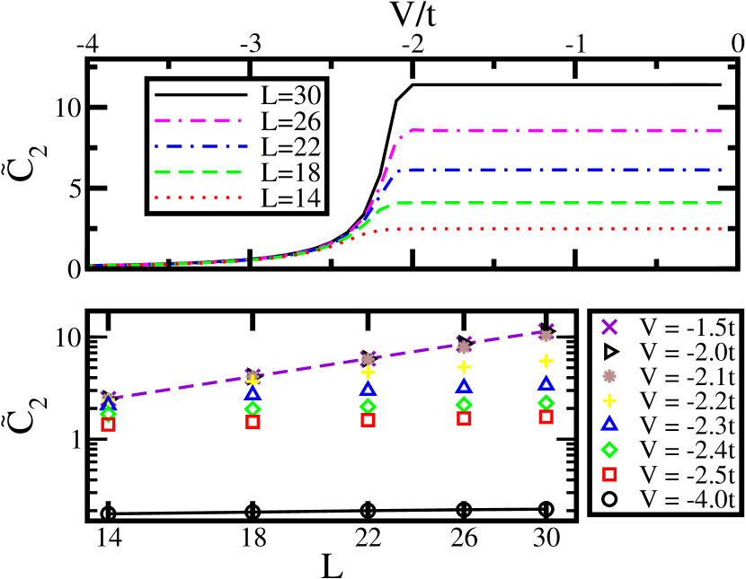
Figure 1: (Color online) Upper panel: $\tilde{C}_{2}$ as a function of $V/t$ for different system sizes. Lower panel: $\tilde{C}_{2}$ as a function of system size for different values of $V$ on a log-log plot. The two lines indicate fits of the function $f(L)=aL^{\gamma}+b$ for the two cases $V=-4.0t$ and $V=-1.5t$.

II Discrete formulas for moments and cumulants

For a system periodic in $L$ we first define the quantity

$$F_{q}=\langle\Psi|\exp(i2\pi q\hat{X}/L)|\Psi\rangle,$$ (1)

where $\hat{X}=\sum_{j=1}^{N}x_{j}\hat{n}_{j}$ . In terms of $F_{q}$ the $n$th moment can be written as

$$M_{n}=\left(\frac{L}{2\pi i}\right)^{n}\left[F_{q}\right]_{q=0}^{(n)}$$ (2)

or the $n$th cumulant as

$$C_{n}=\left(\frac{L}{2\pi i}\right)^{n}\left[\ln F_{q}\right]_{q=0}^{(n)}.$$ (3)

In the above equations the notation $[f_{q}]_{q=0}^{(n)}$ means discrete derivative (finite difference) of order $n$ of the function $f_{q}$ at $q=0$. In a periodic system $q$ take only integer values. Note that Eqs. (2) and (3) amount to interpreting the quantity $F_{q}$ as a discretized characteristic function. It is easily verified that the Resta Resta98 and Resta-Sorella Resta99 formulas for the first and second cumulants, respectively, are reproduced from Eq. (3). Zak also wrote Zak00 an expression for the polarization, which corresponds to $M_{1}$ in a symmetric finite difference approximation.

Below we calculate cumulants by first obtaining the total position $C_{1}$ and redefining $F_{q}$ as follows

$$F_{q}=\langle\Psi|\exp(i2\pi q\hat{X}/L)|\Psi\rangle\exp(-i2\pi qC_{1}/L).$$ (4)

This step is a mere a shift in the coordinate system, and is for numerical convenience. (Cumulants of order greater than one are independent of the average.) We then take the derivative of $\ln F_{q}$ with respect to $F_{q}$ analytically, resulting in a sum of products of moments, and then express the moments via discrete derivatives. For example, the second cumulant is

$$\tilde{C}_{2}=M_{2},$$ (5)

where $M_{2}$ is are given by Eq. (2). $M_{1}$ is zero due to the shift by $C_{1}$. The finite difference derivative expressions in this case are correct up to $\mathcal{O}(L^{-2})$.

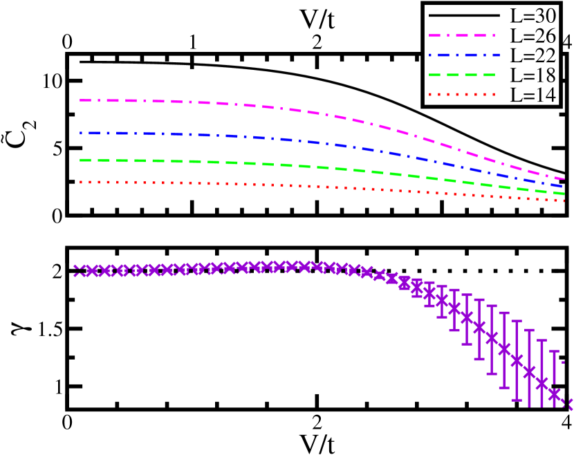
Figure 2: (Color online) Upper panel: $\tilde{C}_{2}$ as a function of $V/t$ for different system sizes. Lower panel: scaling exponent $\gamma$ as a function of $V/t$. The black dotted line indicates the value of two. The error bars were multiplied by ten to make them more visible.

We now show that in a non-interacting framework Eqs.(1) to (3) reproduce the GICs derived by SWM. Souza00 We also derive the criterion which connects Eq. (1) with the characteristic function of the distribution corresponding to the Wannier function, also in a non-interacting system. The derivation is based on the work of Resta. Resta98

Consider a crystalline system of lattice constant $a$ with periodic boundary conditions over $M$ cells ($L=Ma$), leading to $M$ equally spaced Bloch vectors,

$$k_{s}=\frac{2\pi}{Ma}s,\hskip 28.45274pts=0,...,M-1.$$ (6)

The Bloch functions take the form

$$\psi_{k_{s},m}(x)=\exp(ik_{s}x)u_{k_{s},m}(x),$$ (7)

where $u_{q_{x},m}(x)$ is Bloch function periodic in $a$, and $m$ is a band index. There are $N/M$ occupied bands in the ground state wave function, which can be written

$$\Psi_{0}={\bf A}\prod_{m=1}^{N/M}\prod_{s=0}^{M-1}\psi_{k_{s},m},$$ (8)

where ${\bf A}$ is the antisymmetrizer. We now evaluate $F_{q}$ for this wave function,

$$F_{q}=\langle\Psi_{0}|\exp(i2\pi q\hat{X}/L)|\Psi_{0}\rangle=\mbox{det}S,$$ (9)

where

$$S_{sm,s^{\prime}m^{\prime}}=\int_{0}^{L}dx\hskip 2.84544pt\psi^{*}_{k_{s},m}(x)\exp\left(i\frac{2\pi}{L}qx\right)\psi_{k_{s^{\prime}},m^{\prime}}(x).$$ (10)

We used the fact that the overlap of determinants equals the determinant of overlaps. Due to the orthogonality properties of the Bloch wave functions $S_{sm,s^{\prime}m^{\prime}}$ is only finite if $s=s^{\prime}+q$, and $F_{q}$ determinant becomes

$$F_{q}=\prod_{s=0}^{M-1}\mbox{det}S(k_{s},k_{s+q}).$$ (11)

where

$$S_{m,m^{\prime}}(k_{s},k_{s+q})=\int_{0}^{L}dx\hskip 2.84544pt\psi^{*}_{k_{s},m}(x)\exp\left(i\frac{2\pi}{L}qx\right)\psi_{k_{s+q},m^{\prime}}(x).$$ (12)

In terms of the periodic Bloch functions, the matrix $S(k_{s},k_{s+q})$ becomes

$$S_{m,m^{\prime}}(k_{s},k_{s+q})=\int_{0}^{L}dx\hskip 2.84544ptu^{*}_{k_{s},m}(x)u_{k_{s+q},m^{\prime}}(x).$$ (13)

The quantity $F_{q}$ is the moment generating function, whereas $\ln F_{q}$ is the cumulant generating function. Taylor expanding $\ln F_{q}$ in $k_{s+q}-k_{s}=2\pi q/L$ and taking the limit $L\rightarrow\infty$ gives the GICs of SWM (see Eqs. (32) and (33) of Ref. Souza00, ). For example, taking the second derivative of $F_{q}$ in Eq. (11) and the limit $L\rightarrow\infty$ we obtain

$$C_{2}=-\frac{1}{2\pi}\int_{BZ}dk(\langle u_{k,m}|\partial^{2}_{k}|u_{k,m}\rangle-\langle u_{k,m}|\partial_{k}|u_{k,m}\rangle^{2}).$$ (14)

We also derive the condition under which the moments or GICs correspond to the true moments or cumulants of the total position in a band system. The same derivation was used by Zak Zak89 to show that the Zak phase corresponds to the expectation value of the position over the Wannier function of a given band. Using the definition of the Wannier function

$$u_{k,m}(x)=\sum_{p=-\infty}^{\infty}\exp\left(ik(pa-x)\right)a_{m}(x-pa),$$ (15)

we can rewrite the matrix elements as

$$S_{m,m^{\prime}}(k_{s},k_{s+q})=\sum_{p=-\infty}^{\infty}\sum_{p^{\prime}=-\infty}^{\infty}\int_{0}^{L}dx$$ (16)

$$\exp\left(-ik_{s}(pa-x)\right)a^{*}_{m}(x-pa)$$

$$\exp\left(ik_{s+q}(p^{\prime}a-x)\right)a_{m^{\prime}}(x-p^{\prime}a).$$

We can extend the range of the integral to infinity and after further rearrangements obtain

$$S_{m,m^{\prime}}(k_{s},k_{s+q})=\sum_{\Delta p=-\infty}^{\infty}\exp\left(-ik_{s}\Delta pa\right)$$ (17)

$$\int_{-\infty}^{\infty}dx\hskip 2.84544pta^{*}_{m}(x-\Delta pa)a_{m^{\prime}}(x)\exp\left(-i\frac{2\pi}{Ma}qx\right),$$

where $\Delta p=p-p^{\prime}$. Assuming that the overlap between Wannier functions centered in different unit cells is negligible, the matrix elements become

$$S_{m,m^{\prime}}(k_{s},k_{s+q})=\int_{-\infty}^{\infty}dx\hskip 2.84544pta^{*}_{m}(x)a_{m^{\prime}}(x)\exp\left(-i\frac{2\pi}{Ma}qx\right).$$ (18)

In this case $F_{q}=\prod_{s=0}^{M-1}\mbox{det}S(k_{s},k_{s+q})$ is the characteristic function of the squared modulus of the determinant of Wannier functions corresponding to occupied bands. Note that a similar approximation was derived in Ref. Yahyavi17, .

The moments derived above were used to construct the maximally localized Wannier functions Marzari97 ; Marzari12 by optimizing the variance of the position. For a non-interacting system, when the thermodynamic limit is taken, the resulting variance (constructed out of moments) is not gauge invariant. However, one can apply an arbitrary phase to the full many-body wave function in Eqs. (1) and (2) without changing $M_{n}$. In other words, the lack of gauge invariance manifests in the case of separable wave functions, for example, product states of single-particle wave functions, when individual orbitals can take arbitrary phases.

III Interacting model of spinless fermions with nearest neighbor interaction

We study an interacting model of spinless fermions on a lattice in one dimension with Hamiltonian

$$H=\sum_{i=1}^{L}[-t(c^{\dagger}_{i+1}c_{i}+c^{\dagger}_{i}c_{i+1})+Vn_{i}n_{i+1}].$$ (19)

We solve this system via exact diagonalization at half-filling. Our calculations include systems with periodic boundary conditions at half-filling with an odd number of particles (the ground state according to the Perron-Frobenius theorem). At half filling, this model exhibits a transition at $V=2t$ and at $V=-2t$. The former is a continuous transition between a LL at small $V/t$ and a CDW at large $V$, the latter is first-order. For $2t>-V$ the system is also LL, while for $2t<-V$ the ground state is phase separated with particles tending to cluster near each other. In the large $V$ limit the ground state is one in which all particles form a single cluster. This state is highly degenerate, such a state can be displaced by an arbitrary number of sites resulting in states with the same energy.

III.1 Finite size scaling of cumulants

$\tilde{C}_{2}$ is shown in Fig. 1 for the attractive case. The upper panel shows this quantity as a function of $V/t$, while the lower one for fixed values of $V/t$ as a function of system size. In the upper panel, the cumulant increases until the phase transition point, but then levels off to a constant value in the conducting phase. The scaling exponent is difficult to determine in a region close $V=-2t$ in the insulating phase, but it is $\gamma=0.0$ far from the transition point (see line fit to data points for $V=-4.0t$ in Fig. 1), and it gives a value of $\gamma=2.0$ (see line fit to data points for $V=-1.5t$ in Fig. 1) in the conducting phase. Even for values of $V$ closer to the transition point, $\tilde{C}_{2}$ tends to level off to a constant value for larger system sizes, indicating a scaling exponent of $\gamma=0.0$ (see Fig. 1, data for $V=-2.5t$, $V=-2.4t$).

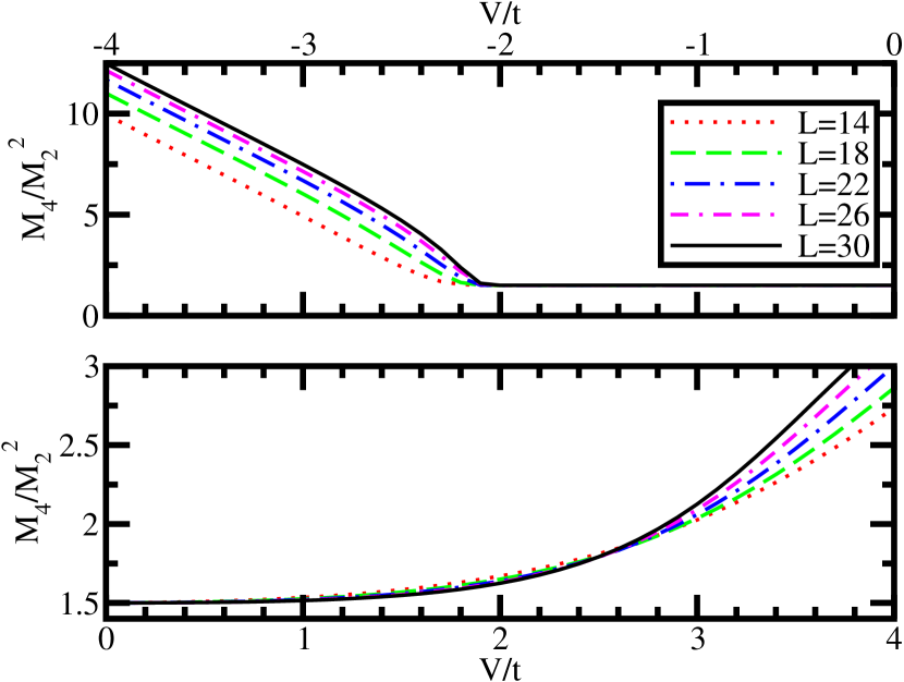
Figure 3: Upper panel(Lower panel): moment ratio $M_{4}/M_{2}^{2}$ for the attractive(repulsive) case.

On the repulsive side, the behavior of these quantities is depicted in Fig. 2. In the upper panel, $\tilde{C}_{2}$ is shown. As $V$ increases, the cumulant decreases monotonically, even in the conducting phase ($V/t<2$). What is remarkable is that, inspite of this, the scaling exponent (lower panel) is very close to a value of $2$ throughout the conducting phase, and starts to decrease as a function of $V$ in the insulating phase. The error bars for the scaling exponent are $\mathcal{O}({10^{-4}})$ in the LL phase, increase around the known phase transition point by several orders of magnitude, until $V/t=3.7$ where they reach a maximum, and start to decrease, indicative of the significant shifting and smearing of the KT transition for these system sizes.

We can connect the fact that in the metallic phase the scaling exponent of the second cumulant with $\gamma$ is two, and decreases when the system enters the insulating phase. It is well-known Chiappe18 that the polarizability obeys precisely this scaling behavior, and the second cumulant gives an upper bound Baeriswyl00 to the polarizability.

\psfrag{x}{$x$}\psfrag{F}{$F$}\psfrag{V/t}{$V/t$}\includegraphics[width=433.62pt,keepaspectratio={true}]{heatmap.eps}

Figure 4: (Color online) Fourier transform of $F_{q}$ as a function of $x$ and the coupling constant $V/t$.

Comparing with the results of Ref. Kobayashi18, we see the advantage of using the cumulants for thermodynamic scaling. There it was determined that $F_{q}\approx L^{\beta(V)}$ for this model, meaning that the scaling of $F_{q}$ depends on the interaction. However, the scaling of $\tilde{C}_{2}$ within the metallic phase is independent of $V$. The scaling exponent $\beta(V)$ is the leading scaling exponent in $F_{q}$ which was found to be linear in $q$ for a number of models. In our definition of the cumulant, we take the derivative of $\ln F_{q}$ analytically with respect to $F_{q}$ (which still results in derivatives of $F_{q}$). For $\tilde{C}_{2}$ two derivatives in $q$ make $\beta{V}$ disappear, so the scaling we find is unaffected by it. We find the expected scaling of the variance of the total position in the LL phase (Figs. 1 and 2) throughout the entire metallic region, while in the attractive region Ref. Kobayashi18, reports definite scaling only for $-t<V<0$.

One way to apply the finite size scaling hypothesis Fisher72 to critical phenomena makes use of the Binder cumulant Binder81 ; Binder92 . One can locate the phase transition point by calculating, for example,

$$U_{4}=1-\frac{\langle\Phi^{4}\rangle}{\langle\Phi^{2}\rangle\langle\Phi^{2}\rangle},$$ (20)

where $\langle\Phi^{m}\rangle$ denotes the $m$th moment of the observable $\Phi$ (the order parameter) for different system sizes as a function of the external parameter under scrutiny, and look for the crossing point of these curves. The essential point is that the product of the powers in the numerator and denominator in the second term are equal. This method has even been applied to locate phase transition points driven by quantum fluctuations Hetenyi99 , but only in cases where the order parameter is an expectation value of an observable, rather than a Berry phase. In this spirit, we calculated $M_{4}/M_{2}^{2}$ (shown in Fig. 3). On the attractive side, in the insulating phase, this quantity has a negative slope as a function of $V$ and exhibits size dependence, while in the conducting phase it is constant and size independent. On the repulsive no size dependence is found until $V/t\approx 2$, but size dependence is found in the insulating phase.

III.2 Total polarization distribution

In Fig. 4 we show the Fourier transform of $F_{q}$ ($\tilde{F}_{x}$) as a function of the variable conjugate to $q$ (denoted by $x$) and the coupling $V$ for a system of size $L=30$. Near $V=0$ $\tilde{F}_{x}$ is flat. Structure begins to develop near $V=\pm 2t$, but much slower on the positive side. The structure eventually consists of two sharp peaks in the region shown, one at half of the lattice, the other at its edge. The fact that there are two is a clear consequence of the filling correction suggested by Aligia and Ortiz Aligia99 . It is interesting that the behavior of this quantity, which is related to the distribution of the center of mass, behaves similar on both $\pm V$, even though the nature of the ground states are very different. In the extreme limits, $V\rightarrow\pm\infty$ one can easily construct the probability distributions for ground states (perfect CDW for $V\rightarrow\infty$, all particles “stuck” together for $V\rightarrow-\infty$).

To show this, let $N$ denote the number of particles, and $L$ the number of lattice sites, and $L/N=2$. At large and positive $V$ the CDW state is doubly degenerate, we can write the expectation value of $\hat{X}$ for each of these as:

$$X_{+}=\sum_{j=1}^{N}(2j-1)=N^{2}$$ (21)

$$X_{-}=\sum_{j=1}^{N}(2j)=N^{2}+N,$$ (22)

each occurring with a probability of one-half. Since the operator $\exp(i2\pi q\hat{X}/L)$ is diagonal in the position representation we can write

$$F_{q}=\frac{1}{2}\left(e^{i\frac{2\pi q}{L}N(N+1)}+e^{i\frac{2\pi q}{L}N^{2}}\right)=\begin{cases}1&\mbox{if $q$ is even}\\ 0&\mbox{if $q$ is odd.}\end{cases}$$ (23)

For the case of extreme clustering ($V\rightarrow-\infty$) the ground state is $L$-fold degenerate. The expectation values of the total position are

$$X_{k}=Nk+\sum_{j=1}^{N}j=Nk+\frac{N(N+1)}{2},$$ (24)

where $k$ corresponds to the $k$th degenerate ground state. In this case, $F_{q}$ becomes

$$F_{q}=\frac{1}{L}\sum_{k=0}^{L-1}e^{i\frac{2\pi}{L}q\left[Nk+\frac{N(N+1)}{2}\right]}.$$ (25)

It is easily shown, using that $N=L/2$ is odd that again we have

$$F_{q}=\begin{cases}1&\mbox{if $q$ is even}\\ 0&\mbox{if $q$ is odd.}\end{cases}$$ (26)

\psfrag{x}{$x$}\psfrag{F}{$F$}\psfrag{V/t}{$V/t$}\includegraphics[width=433.62pt,keepaspectratio={true}]{gamV4.eps}

Figure 5: (Color online) Upper panel: $\tilde{C}_{2}$ as a function of $V^{\prime}/t$ for a system of fermions with nearest and next-nearest neighbor interaction for the case $V=4t$. Four system sizes are shown, $L=22,24,26,28$. Lower panel: Size scaling exponent $\gamma$ for $\tilde{C}_{2}$ as a function of $V^{\prime}/t$. Diamonds show the results based on calculations for systems with sizes $L=4m$, where $m$ is an integer ($L=12,16,20,24,28$), left triangles show the results based on calculations for system sizes $L=4m-2$, where $m$ is an integer ($L=10,14,18,22,26$). The dotted line indicates the value of two. $V_{c}^{\prime}\approx 1.0$ is the critical point for the transition between the charge-density wave and the Luttinger liquid phases. $V_{c}^{\prime}\approx 2.9$ is the critical point for the transition between the Luttinger liquid and the bond-order phases.

IV Interacting model of spinless fermions with nearest and next nearest neighbor interaction

The other model we study is an interacting model of spinless fermions on a lattice in one dimension with Hamiltonian

$$H=\sum_{i=1}^{L}[-t(c^{\dagger}_{i+1}c_{i}+c^{\dagger}_{i}c_{i+1})+Vn_{i}n_{i+1}+V^{\prime}n_{i}n_{i+2}].$$ (27)

The phase diagram of this model was determined by Mishra et al. Mishra11 In addition to the two phases already known (LL and CDW) two more phases were found; a bond order (BO) phase at intermediate $V^{\prime}$ and another charge-density wave (CDW-2) phase for large $V^{\prime}$. The latter consists of alternating pairs of particles and pairs of holes. As $V^{\prime}\rightarrow\infty$ the ordered state that emerges is one which pairs of particles alternate with pairs of holes. We may write the four possible ordered states as

$$X_{1} = \sum_{j=1}^{\frac{N}{2}}(4j-3)+\sum_{j=1}^{\frac{N}{2}}(4j-2),$$ (28)

$$X_{2} = \sum_{j=1}^{\frac{N}{2}}(4j-2)+\sum_{j=1}^{\frac{N}{2}}(4j-1),$$

$$X_{3} = \sum_{j=1}^{\frac{N}{2}}(4j-1)+\sum_{j=1}^{\frac{N}{2}}(4j),$$

$$X_{4} = \sum_{j=1}^{\frac{N}{2}}(4j)+\sum_{j=1}^{\frac{N}{2}}(4j-3).$$

Using these ordered states it can be shown that

$$F_{q}=\begin{cases}-1&\mbox{if $q$ is even}\\ 0&\mbox{if $q$ is odd.}\end{cases}$$ (29)

We see that a sign change occurs between the two CDW phases (compare with Eq. (23)) corresponding to a shift of the maximum of the polarization.

In Fig. 5 we present our results for $\tilde{C}_{2}$ (upper panel) and its finite size scaling exponent (lower panel) for $V=4t$ as a function of $V^{\prime}/t$. In Ref. Mishra11, it was found that the CDW to LL transition occurs at $V_{c}^{\prime}\approx 1.0t$, while the LL to BO at $V_{c}^{\prime}\approx 2.9t$ The BO phase transforms into the second CDW phase at $V_{c}^{\prime}\approx 4.29t$. Other than the LL all other phases are gapped and insulating. In Ref. Mishra11, Fig. 3 shows the gap for this case, which is zero in the region $1.0t<V^{\prime}<2.9t$, exactly where the scaling exponent $\gamma=2$ (Fig. 5 lower panel). Thus, phase transitions accompanied by gap closure (metal-insulator transitions) can be detected by our method.

While transitions between gapped to gapped phases are more difficult, in this case the BO to CDW-2 transition can be approximately located based on comparing calculations for systems of size $L=4m$ and $L=4m-2$ ($m$ integer), since the ordered CDW-2 unit cell is four lattice sites. In the upper panel it is obvious that $\tilde{C}_{2}$ converges to different values for $L=24,28$ from those of $L=26,22$. The two sets of curves start to deviate at $V^{\prime}<4.29t$, since it is expected that the correlations associated with CDW-2 persist in the BO phase. It is interesting that the scaling exponents for $L=4m$ and $L=4m-2$ deviate significantly only after $V^{\prime}\approx 4.3t$.

V Conclusion

Even though the polarization in crystalline systems corresponds to a Berry phase, proper finite size scaling is possible via discrete formulas for gauge invariant cumulants. The variance of the polarization in hte Luttinger liquid (gapless) phase exhibit a finite size-scaling exponent $\gamma=2$. Based on this we were able to identify metal-insulator transitions in several interacting models. The main limitation in our study appears to be the small system sizes accessible to exact diagonalization.

References

- (1) R. D. King-Smith and D. Vanderbilt, Phys. Rev. B 47 1651 (1993).
- (2) R. Resta, Rev. Mod. Phys. 66 899 (1994).
- (3) M. V. Berry, Proc. Roy. Soc. London A392 45 (1984).
- (4) D. Xiao, M.-C. Chang, and Q. Niu, Rev. Mod. Phys. 82 1959 (2010).
- (5) J. Zak, Phys. Rev. 62 2747 (1989).
- (6) B. A. Bernevig and T. L. Hughes, Topological Insulators and Topological Superconductors Princeton University Press, 2013.
- (7) D. J. Thouless, M. Kohmoto, M. P. Nightingale, and M. den Nijs Phys. Rev. Lett 49 405 (1982).
- (8) D. J. Thouless Phys. Rev. B 27 6083 (1983).
- (9) L. Fu and C. L. Kane, Phys. Rev. B 74 195312 (2006).
- (10) I. Souza, T. Wilkens, and R. M. Martin, Phys. Rev. B 62 1666 (2000).
- (11) R. Resta, Phys. Rev. Lett. 80 1800 (1998).
- (12) R. Resta and S. Sorella, Phys. Rev. Lett. 82 370 (1999).
- (13) A. A. Aligia and G. Ortiz, Phys. Rev. Lett. 82 2560 (1999).
- (14) M. Nakamura and J. Voit, Phys. Rev. B 65 153110 (2002).
- (15) M. Oshikawa, Phys. Rev. Lett. 90 236401 (2003).
- (16) W. Kohn, Phys. Rev. 133 A171 (1964).
- (17) M. E. Fisher and M. N. Barber, Phys. Rev. Lett. 28 1516 (1972).
- (18) K. Binder, Phys. Rev. Lett. 47 693 (1981).
- (19) K. Binder, Annu. Rev. Phys. Chem. 43 33 (1992).
- (20) R. Kobayashi, Y. O. Nakagawa, Y. Fukusumi, M. Oshikawa, Phys. Rev. B 97 165133 (2018).
- (21) H. Watanabe and M. Oshikawa, Phys. Rev. X 8 021065 (2018).
- (22) M. Nakamura, arXiv:1807.02864.
- (23) E. Lieb, T. Schultz, and D. Mattix, Ann. Phys. (N.Y.) 16 407 (1961).
- (24) B. Hetényi, Phys. Rev. B 87 235123 (2013).
- (25) S. Patankar, L. Wu, M. Rai, J. D. Tran, T. Morimoto, D. E. Parker, A. G. Grushin, N. L. Nair, J. G. Analytis, J. E. Moore, J. Orenstein, D. H. Torchinsky, P hys. Rev. B 98 165113 (2018).
- (26) M. Yahyavi and B. Hetényi, Phys. Rev. A 95 062104 (2017).
- (27) G. Chiappe, E. Louis, J. A. Vergés, J. Phys. Cond. Mat. 30 175603 (2018).
- (28) D. Baeriswyl, Found. Phys. 30 2033 (2000).
- (29) J. Zak, Phys. Rev. Lett. 85 1138 (2000).
- (30) N. Marzari and D. Vanderbilt, Phys. Rev. B 56 12847 (1997).
- (31) N. Marzari et al., Rev. Mod. Phys. 84 1419 (2017).
- (32) B. Hetényi, M. H. Müser, and B. J. Berne, Phys. Rev. Lett. 83 4606 (1999).
- (33) T. Mishra, J. Carrasquilla, M. Rigol, Phys. Rev. B 84 115135 (2011).