Flow Past a Circular Cylinder on Curved Surfaces

Abstract

We investigate the dynamics of flows past a stationary circular cylinder embedded on spherical and cylindrical surfaces at a fixed Reynolds number of 100. For flows on surfaces, it is convenient to express the Navier-Stokes equations in exterior calculus notation. We employ the discrete exterior calculus (DEC) method (Mohamed et al. (2016)) to numerically solve the equations. We explore the role played by curvature on dynamical quantities of interest: the drag coefficient $\left(C_{d}\right)$, the lift coefficient $\left(C_{l}\right)$, and the Strouhal number $\left(St\right)$. Our simulations indicate that the effect of surface curvature on these quantities and the overall flow dynamics is somewhat insignificant thereby implying that the dynamics of the flow past a stationary circular cylinder exhibits universality, independent of the embedding surface geometry.

¹ Mechanical Engineering, Physical Science and Engineering Division, King Abdullah University of Science and Technology, Thuwal, Saudi Arabia

²Department of Mechanical Design and Production, Faculty of Engineering, Cairo University, Giza, Egypt

1 Introduction

Research on the dynamics of flow past a circular cylinder dates back to the century old discovery of Kármán vortex street (Von Kármán (1912)). Some of the classic studies on this topic include works by Kármán, Taylor and others (Von Kármán (1912); Taylor (1915); Wieselsberger (1921); Fage (1929); Thom (1933)). Comprehensive reviews of the literature on this topic are available in Niemann and Hölscher (1990); Rao et al. (2015). It is evident from the literature that the dynamics of the flow past a cylinder embedded on a flat surface have been extensively studied. One may pose the following question: what, if any, are the changes to the dynamics of flow past a circular cylinder embedded on a curved surface? So far a clear exploration of this question has not been undertaken. This research problem is not only of academic interest, but also motivated by applications related to geophysical flows.

In order to explore the research question expressed above, it is essential to have a robust numerical method with certain desirable conservation and mimetic properties. One such method is discrete exterior calculus (DEC). DEC is a mimetic method that retains, at the discrete level, many of the rules/identities of its continuous counterparts (Hirani (2003); Desbrun et al. (2005)). This results in superior conservation properties for DEC discretization of physical problems. For example, many DEC-based discretizations of the incompressible Navier-Stokes equations are known to exactly conserve mass, vorticity and kinetic energy (Mullen et al. (2009); Mohamed et al. (2016)). This makes such discretizations appropriate for investigating vortex dynamics and flows dominated by long-lived coherent structures. Moreover, DEC is coordinate independent and therefore convenient to investigate flows over arbitrary curved surfaces/manifolds.

Here, we present a study of the dynamics of flows past a stationary cylinder embedded on spherical and cylindrical surfaces. The DEC scheme developed by Mohamed et al. (2016) is used to perform the simulations. Surfaces comprising of different curvatures are employed, and the curvature effect on the flow dynamics is evaluated at a fixed Reynolds number ($Re=100$). A brief outline of this paper is as follows. The details of the physical setup, computational domain are in section 2. The governing equations in the DEC framework are described in section 3. The results are discussed in section 4. The key outcomes of the study are finally summarized in section 5.

2 Physical Setup and Computational Domain

The schematic of the physical setup and computational domain are shown in figures 1a and 1b for the case of spherical and cylindrical surfaces, respectively. The circular cylinder contour embedded on the curved surfaces is generated by intersecting a cylinder of diameter D = 1 with the spherical and cylindrical surfaces. In terms of geodesic distances, the domain lengths upstream and downstream of the cylinder are 10D and 60D, respectively. The domain width on either side of the cylinder is 10D. These domain sizes are typical of computational investigations of flow past a cylinder on a flat surface. The implemented boundary conditions are shown in figure 1 for each domain boundary, where $u$ and $v$ for a specific boundary represent the local normal and tangential velocity components. The radii of the embedding surfaces employed are reported in table 1.

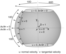
(a) Spherical surface

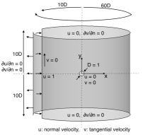
(b) Cylindrical surface

Figure 1: Schematic of the computational domain for both spherical and cylindrical surfaces showing the domain dimensions and the boundary conditions. Velocity components ($u,v$) indicate normal and tangential velocity components to the boundary.

3 Numerical Procedure

The numerical scheme is discussed here only briefly, and the reader may refer to Mohamed et al. (2016) for more details. Unlike the stream function formulation employed in Mohamed et al. (2016), the present simulations adopts the primitive variable formulation. The Navier-Stokes equations, in exterior calculus notation, are expressed as

$$\frac{\partial\mathbf{u}}{\partial t}-\mu\ast d\ast d\mathbf{u}-2\mu\kappa\mathbf{u}+\ast\left(\mathbf{u}\wedge\ast d\mathbf{u}\right)+dp^{d}=0,$$ (1)

$$\ast d\ast\mathbf{u}=0,$$ (2)

The reference for these equations is Mohamed et al. (2016). Note the presence of the term $2\mu\kappa\mathbf{u}$ : this is Gaussian curvature term which results from the divergence of the deformation tensor and the non-commutativity of the second covariant derivative in curved spaces (Nitschke et al. (2017)). Here, $\mathbf{u}$, $\kappa$, $\mu$, $\ast$, $d$, $\wedge$, and $p^{d}$ denote the velocity 1-form, Gaussian curvature, dynamic viscosity, Hodge star, exterior derivative, wedge product, and dynamic pressure 0-form, respectively.

Considering the primal mesh, for the domain discretization, and the corresponding dual mesh, equation (1) in DEC notation reads

$$\frac{U^{n+1}-U^{n}}{\triangle t}-\mu\ast_{1}d_{0}\ast_{0}^{-1}\left[\left[-d_{0}^{T}\right]U+d_{b}V\right]-2\mu\kappa U+\ast_{1}W_{V}\ast_{0}^{-1}\left[\left[-d_{0}^{T}\right]U+d_{b}V\right]+d_{1}^{T}P^{d}=0.$$ (3)

Here, the choice of the velocity 1-form $\mathbf{u}$ represents the velocity integration on the dual edges, except at the first position in the wedge product where the choice has to be on the primal edge (this choice represents tangential velocity 1-form $\mathbf{v}$) for consistency (Mohamed et al. (2016)). $U$, $V$, and $P^{d}$ are vectors representing the discrete dual velocity 1-forms for all mesh dual edges, the primal velocity 1-forms for all mesh primal edges, and the dynamic pressure dual 0-forms for all mesh dual vertices, respectively. The discrete time interval is expressed as $\Delta t$. The $W_{V}$ matrix represents the discrete wedge product of the tangential velocity 1-form with the 0-form *du (as in equation (1)) and contains the values of the tangential velocity 1-form. The operation $\left[-d_{0}^{T}\right]U$ evaluates the circulation of the velocity forms $\mathbf{u}$ along the dual 2-cells boundaries. The operation $d_{b}V$ complements the velocity circulation since a portion of the dual 2-cells boundaries may consists of primal edges, and accounts for the part that depends on the velocity 1-forms $\mathbf{v}$ on the primal boundary edges. The discrete operators $\ast_{1}$, $d_{0}$, $\ast_{0}^{-1}$, $\left[-d_{0}^{T}\right]$, $d_{b}$, $W_{V}$, and $d_{1}^{T}$ are described in detail in Reference Mohamed et al. (2016), and not repeated here for the sake of brevity. Let $U^{\ast}$ be the vector containing mass flux primal 1-form $u^{\ast}$ for all mesh primal edges. We then have $U^{*}=-\ast_{1}^{-1}U$ and $U=\ast_{1}U^{\ast}$. After this substitution, equation (3) can be rewritten as

$$\ast_{1}\left[\frac{\left(U^{*}\right)^{n+1}-\left(U^{*}\right)^{n}}{\triangle t}\right] -\mu\ast_{1}d_{0}\ast_{0}^{-1}\left[\left[-d_{0}^{T}\right]\ast_{1}U^{*}+d_{b}V\right]-2\mu\kappa\ast_{1}U^{\ast}$$ (4)

$$+\ast_{1}W_{V}\ast_{0}^{-1}\left[\left[-d_{0}^{T}\right]\ast_{1}U^{*}+d_{b}V\right]+d_{1}^{T}P^{d}=0.$$

Applying the Hodge star operator $\ast_{1}^{-1}$ to equation (4), and considering the property $\ast_{1}^{-1}\ast_{1}=-1$, we have

$$-\frac{\left(U^{*}\right)^{n+1}-\left(U^{*}\right)^{n}}{\triangle t} +\mu d_{0}\ast_{0}^{-1}\left[\left[-d_{0}^{T}\right]\ast_{1}U^{*}+d_{b}V\right]+2\mu\kappa U^{\ast}$$ (5)

$$-W_{V}\ast_{0}^{-1}\left[\left[-d_{0}^{T}\right]\ast_{1}U^{*}+d_{b}V\right]+\ast_{1}^{-1}d_{1}^{T}P^{d}=0.$$

In the above equation, the viscous and curvature terms are treated implicitly, while the convection term is treated explicitly. Hence, we write

$$\left[-\frac{1}{\triangle t}I+\mu d_{0}\ast_{0}^{-1}\left[-d_{0}^{T}\right]\ast_{1}+2\mu\kappa I\right]\left(U^{*}\right)^{n+1}+\ast_{1}^{-1}d_{1}^{T}\left(P^{d}\right)^{n+1}=F,$$ (6)

with

$$F=\frac{1}{\triangle t}\left(U^{*}\right)^{n}-\mu d_{0}\ast_{0}^{-1}d_{b}V^{n}+W_{V}^{n}\ast_{0}^{-1}\left[\left[-d_{0}^{T}\right]\ast_{1}\left(U^{*}\right)^{n}+d_{b}V^{n}\right].$$ (7)

The continuity equation is expressed as

$$\left[d_{1}\right]\left(U^{*}\right)^{n+1}+\left[0\right]\left(P^{d}\right)^{n+1}=0.$$ (8)

Equations (6) - (8) form a linear system of equations with $U^{\ast}$ and $P^{d}$ at time $(n+1)$ to be the mass flux and dynamic pressure unknown degrees of freedom. This linear system is solved along with the boundary conditions depicted in figure 1.

The computational domain is discretized using a triangular mesh. A representative computational mesh comprising of 80,008 nodes and 159,280 elements is shown in figure 2. Figure 2a shows the mesh for the whole domain, whereas figure 2b shows close up view around the cylinder. The nodes and elements for the meshes employed are in the range 79,960 - 80,628, and 159,184-160,520, respectively.

4 Results and Discussion

In this section, we present simulation results for flow past a cylinder with the configurations corresponding to (i) spherical surfaces and (ii) cylindrical surfaces, both with surface radii R = 12, 18, 24, 30, 36, and 72, and (iii) a flat surface as a reference. The Reynolds number ($Re=\rho u_{\infty}D/\mu$) is fixed at 100 for all the cases. Here, $\rho$, and $u_{\infty}$ denotes for the fluid density (taken to be unity), and the free stream velocity at the inlet, respectively.

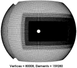
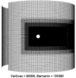
(a) Whole domain

(b) Around the cylinder

Figure 2: A representative computational mesh

The net force acting on the cylinder, due to pressure and viscous terms, is expressed as (Shi et al. (2004))

$$\vec{F}=\int_{S}-p\vec{n}dA+\mu\int_{S}\vec{\omega}\times\vec{n}dA$$ (9)

where $p$ is the static pressure, $\vec{n}$ is the unit normal facing outward of the cylinder, $\vec{\omega}$ is the vorticity vector, $dA$ is an infinitesimal area (actually are lengths), and $S$ denotes for the total surface area of the cylinder. Since the boundary corresponding to the cylinder wall is discretized with $N$ mesh edges, the discrete expression of the force vector is

$$\vec{F}=\sum_{k=1}^{N}-p_{k}\vec{n}_{k}l_{k}+\mu\sum_{k=1}^{N}l_{k}\vec{\omega}_{k}\times\vec{n}_{k}$$ (10)

where the summation is over the cylinder boundary edges. Here, we consider the global $(x,y,z)$ coordinate system with the cylinder axis intersection with the surface as the origin, the cylinder axis along the z-direction, and the x and y directions as shown in figure 1. The pressure $p_{k}$ is the static pressure in the neighbor triangle, $\vec{n}_{k}$ is the unit vector normal to the edge (projected on the x-y plane), and $l_{k}$ is the edge length. For the case of 2D surfaces, the vorticity is calculated as a scalar on the primal mesh nodes (Mohamed et al. (2016)). The vector $\vec{\omega}_{k}=\vec{n}_{k,s}|\omega_{k}|$, with $\vec{n}_{k,s}$ denoting the unit normal facing outward to the surface at the edge midpoint. The vorticity magnitude $|\omega_{k}|$ is calculated by averaging the vorticity on both nodes of the edge. The drag force $F_{d}$ and the lift force $F_{l}$ are respectively the $x$ and $y$ components of the force vector.

The drag coefficient is calculated using the expression $C_{d}=F_{x}/\left(\frac{1}{2}\rho u_{\infty}^{2}D\right)$, where $F_{x}$ denotes for the x-component of the net force on the cylinder. To calculate the lift coefficient, the expression $C_{l}=F_{y}/\left(\frac{1}{2}\rho u_{\infty}^{2}D\right)$ is used, where $F_{y}$ is the y-component of the net force on the cylinder. The Strouhal number is $St=fD/u_{\infty}$, where $f$ is the vortex shedding frequency.

Figure 3 shows the Kármán vortex street in the wake of each cylinder for different radii of the embedding cylindrical or spherical surface. The vortices in magnitude and spacing are similar to those for the flow past a cylinder on a flat surface. The plots of the drag coefficient, $C_{d}$ as a function of time, for a finite time duration after the periodically steady vortex shedding commences, are shown in figures 4a, 4b, and 4c for spherical, cylindrical and flat surfaces, respectively, and the corresponding mean values are reported in table 1. The mean drag coefficient for the flat surface is $1.386$, which is within the range of values reported in the literature (i.e., 1.38 (Russell and Wang (2003)), 1.37 (Le et al. (2006))). For the case of spherical surface, the mean drag coefficient is $1.386$ for $R=72$. The mean drag coefficient decreases slightly with increasing curvature of the surface, and for $R=12$ (the highest curvature case) it is computed to be $1.369$. The change in $C_{d}$ with curvature is about $1\%$ and thus very weakly dependent (or perhaps even independent) of the embedding surface curvature, and the mean drag coefficient almost coincides with that for the flat surface. For the case of embedding cylindrical surface, the mean drag coefficient is constant at $1.386$ coinciding with that for the flat surface. Relative changes in magnitude of $C_{d}$ of about $1\%$ or a few percent are not unexpected when the mesh resolution changes; or a different quadrature used to compute the drag coefficient by integrating the forces on the surface of the cylinder. One may reasonably conclude that the effect of the embedding surface curvature on the drag coefficient is insignificant.

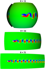
(a) Spherical surface

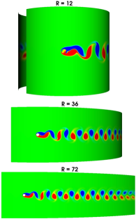
(b) Cylindrical surface

Figure 3: Vortex streets. R denotes radius of the embedding surface.

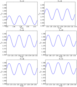
(a) Spherical surface

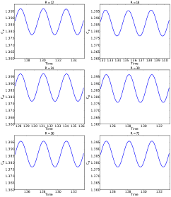
(b) Cylindrical surface

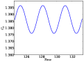
(c) Flat surface

Figure 4: Drag coefficient as a function of time. R denotes radius of the embedding surface

Figures 5a, 5b, and 5c show the lift coefficient as a function of time for the cases of spherical, cylindrical and flat surfaces, respectively. The RMS values of the lift coefficient are reported in table 1. The RMS lift coefficient value is $0.248$ for the flat surface, which is within the range of values reported in the literature. It is computed to to be $0.248$ for the spherical surface of $R=72$ and $0.246$ for $R=12$, i.e. a negligible decrease (less than $1\%$) in the value with changes in curvature of the embedding surface. For the cylindrical surface, all RMS values are constant at $0.248$ coinciding with that for the flat surface. These results suggest insignificant effect of the surface curvature on the lift coefficient RMS value. It is worth noting that there exists a z-component of the net force on the cylinder due to the viscous term, but this is negligibly small for both the spherical and cylindrical embedding surfaces.

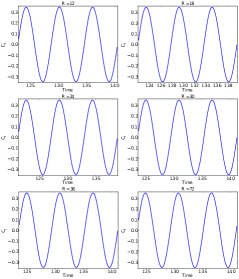
(a) Spherical surface

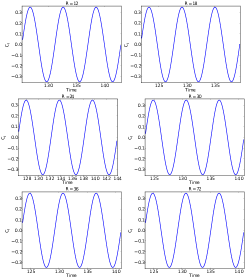
(b) Cylindrical surface

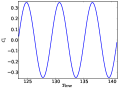
(c) Flat surface

Figure 5: Lift coefficient as a function of time.

The values of shedding frequency or Strouhal number are reported in table 1. For the flat surface, the Strouhal number is computed as $0.171$ which is within the range of values reported in the literature. For the spherical surface, the Strouhal number is $0.171$ for $R=72$. It changes negligibly with the radius, and for $R=12$ it is found to be $0.170$. Thus, it almost coincides with that for the flat surface. The Strouhal number is almost constant at $0.171$ irrespective of the radius for the cylindrical surfaces, which coincides with that for the flat surface. These results suggest the negligible effect of the surface curvature on the Strouhal number.

Surface type	Radius of the surface	$C_{d}$ (mean)	$C_{l}$ (RMS)	$St$
Spherical surface	12	1.369	0.246	0.17
	18	1.379	0.247	0.17
	24	1.383	0.247	0.171
	30	1.384	0.248	0.171
	36	1.384	0.248	0.171
	72	1.386	0.248	0.171
Cylindrical surface	12	1.386	0.248	0.171
	18	1.386	0.248	0.171
	24	1.386	0.248	0.171
	30	1.386	0.248	0.171
	36	1.386	0.248	0.171
	72	1.386	0.248	0.171
Flat surface	Present study	1.386	0.248	0.171
	Russell and Wang (2003)	1.38	-	0.172
	Le et al. (2006)	1.37	-	0.160
	Park et al. (1998)	1.33	0.3321	0.165
	Mittal (2005)	1.322	0.226	0.1644
	Stålberg et al. (2006)	1.32	0.233	0.166
	Posdziech and Grundmann (2001)	1.325	0.228	0.1644
	Li et al. (2009)	1.336	-	0.164
	Qu et al. (2013)	1.319	0.225	0.1648

Table 1: Values of the drag coefficient, the lift coefficient and the Strouhal number.

The pressure coefficient plots $C_{p}=\left(p-p_{\infty}\right)/\left(\frac{1}{2}\rho u_{\infty}^{2}\right)$ as a function of the angular position on the cylinder surface, for all surfaces of different radii as well as the flat surface, are shown in figure 6a, where $p_{\infty}$ denotes the free stream pressure. The plots overlap, which further supports the negligible effect of the surface curvature on the flow dynamics. Similarly, we note the absence of any significant dependence on curvature in the plots of vorticity magnitude $\omega^{\ast}=\omega_{n}D/u_{\infty}$ as a function of the angular position on the cylinder surface as shown in figure 6b, where $\omega_{n}$ is the vorticity in the surface normal direction (considered as a scalar for calculations on surfaces).

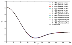
(a) Pressure coefficient

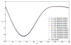
(b) Vorticity magnitude

Figure 6: Pressure coefficient and vorticity magnitude as a function of the angular position on the cylinder surface.

The aforementioned results all suggest that the dynamics of the flow past a stationary circular cylinder embedded on a curved surface is not significantly affected by the surface curvature, and is almost identical to that for a flat surface. In other words, the dynamics of flow past a circular cylinder exhibits universality. For a given embedded cylinder, in addition to the geometry of the embedding surface, there are two other factors that can affect the flow dynamics around the cylinder on a curved surface, the Gaussian curvature term $\left(2\mu\kappa U\right)$ in equation (3) and the departure of the intersection contour between the cylinder and the surface from being a planar circle. In order to quantify the relative magnitude of curvature term influence in the momentum equation, we compared its magnitude with the viscous term magnitude (both terms depend on the fluid viscosity or Reynolds number). For the case of spherical embedding surface, we found that the viscous term ($\mu\ast_{1}d_{0}\ast_{0}^{-1}\left[\left[-d_{0}^{T}\right]U+d_{b}V\right]$) dominates in the region around the cylinder, being almost eight orders of magnitude larger than the curvature term. Therefore, for the simulations considered in the present study, the curvature term in equation (3) has insignificant effect on the flow dynamics around the cylinder. For a cylindrical surface on the other hand, the Gaussian curvature, and therefore the curvature term, is identically equal to zero and does not affect the flow dynamics. Let us now consider the aspect of the domain geometry, i.e., the intersection contour between the cylinder and the embedding surface. For a spherical embedding surface, the intersection is identical to a planar circle. The geometry in the region around the cylinder is therefore not significantly different from that for a flat surface, and does not considerably affect the flow dynamics. On the other hand, for an embedding cylindrical surface, the intersection contour with the cylinder is not planar. However, for the cases considered during the present study, the differences between such intersection contour and a plane circle remains relatively small. This can be quantified by evaluating the maximum variation of the z-coordinate along the intersection contour and also the change in the intersection contour length in comparison to a plane circle, as stated in table 2. The reported values are evidently insignificant. The inconsiderable impact of the curvature term in equation (3) along with the trivial domain geometry changes ultimately resulted in the observed similarity in the flow past a cylinder dynamics on curved surfaces, in comparison to that on a flat surface.

Radius of cylindrical surface	Maximum z – variation	% change in the contour
	along the contour	length when compared
		to that for a flat surface
R = 12	0.01040	0.02419
R = 36	0.00347	0.00477
R = 72	0.00174	0.00318

Table 2: Change in z-coordinate for the intersection contour for cylindrical surfaces

5 Conclusion

In the present study, we have investigated the dynamics of flows past a stationary circular cylinder embedded on spherical and cylindrical surfaces using a DEC-based numerical method at a modest Reynolds number of 100. Various surface curvatures were considered in order to explore the curvature effects on the flow dynamics, and key quantities such as drag, lift coefficients, the vortex shedding frequency, and the magnitude and spacing of the coherent vortices in the wake, are compared with the flow past a cylinder on a flat surface. For a circular cylinder of unit diameter, the embedding spherical and cylindrical surfaces of radii ranging from 12 to 72 were considered. No significant differences were observed in the flow dynamics on the curved surfaces, when compared with the flow on a flat surface. We examined the magnitude of the curvature term in the momentum equation, relative to the other viscous term and found this to be insignificant. In addition, the cylinder contour geometry either is a planar circle as for the case of the embedding spherical surfaces case, or has very minor deviation from a planar circle in the case of the embedding cylindrical surfaces case. The deviation from a planar circle is small enough and the resulting effect on the flow dynamics is also insignificant. A key conclusion is that the dynamics of a flow past a stationary circular cylinder embedded on a surface is not significantly affected by the curvature of the embedding surface, unlike what one may expect based on pure intuition. The following open questions remain: what if the embedding surface curvature was even larger? and how will the results change with increasing Reynolds numbers. We leave exploration of these questions for the future.

References

- Desbrun et al. (2005) Desbrun, M., Hirani, A. N., Leok, M., and Marsden, J. E. (2005). Discrete exterior calculus. arXiv preprint math/0508341.
- Fage (1929) Fage, A. (1929). The effects of turbulence and surface roughness on the drag of a circular cylinder. Rep, Memo., 1283:1.
- Hirani (2003) Hirani, A. N. (2003). Discrete exterior calculus. PhD thesis, California Institute of Technology.
- Le et al. (2006) Le, D., Khoo, B. C., and Peraire, J. (2006). An immersed interface method for viscous incompressible flows involving rigid and flexible boundaries. Journal of Computational Physics, 220(1):109–138.
- Li et al. (2009) Li, Y., Zhang, R., Shock, R., and Chen, H. (2009). Prediction of vortex shedding from a circular cylinder using a volumetric Lattice-Boltzmann boundary approach. European Physical Journal: Special Topics, 171(1):91–97.
- Mittal (2005) Mittal, S. (2005). Excitation of shear layer instability in flow past a cylinder at low Reynolds number. International Journal for Numerical Methods in Fluids, 49(10):1147–1167.
- Mohamed et al. (2016) Mohamed, M. S., Hirani, A. N., and Samtaney, R. (2016). Discrete exterior calculus discretization of incompressible navier–stokes equations over surface simplicial meshes. Journal of Computational Physics, 312:175–191.
- Mullen et al. (2009) Mullen, P., Crane, K., Pavlov, D., Tong, Y., and Desbrun, M. (2009). Energy-preserving integrators for fluid animation. ACM Trans. Graph., 28(3):38.
- Niemann and Hölscher (1990) Niemann, H. and Hölscher, N. (1990). A review of recent experiments on the flow past circular cylinders. Journal of Wind Engineering and Industrial Aerodynamics, 33(1-2):197–209.
- Nitschke et al. (2017) Nitschke, I., Reuther, S., and Voigt, A. (2017). Discrete exterior calculus (dec) for the surface navier-stokes equation. In Transport Processes at Fluidic Interfaces, pages 177–197. Springer.
- Park et al. (1998) Park, J., Kwon, K., and Choi, H. (1998). Numerical solutions of flow past a circular cylinder at Reynolds numbers up to 160. KSME International Journal, 12(6):1200–1205.