Batch-Parallel Euler Tour Trees

Abstract

The dynamic trees problem is to maintain a forest undergoing edge insertions and deletions while supporting queries for information such as connectivity. There are many existing data structures for this problem, but few of them are capable of exploiting parallelism in the batch setting, in which large batches of edges are inserted or deleted from the forest at once. In this paper, we demonstrate that the Euler tour tree, an existing sequential dynamic trees data structure, can be parallelized in the batch setting. For a batch of $k$ updates over a forest of $n$ vertices, our parallel Euler tour trees achieve $O(k\log(1+n/k))$ expected work and $O(\log n)$ depth with high probability. Our work bound is asymptotically optimal, and we improve on the depth bound achieved by Acar et al. for the batch-parallel dynamic trees problem [1].

Our main building block for parallelizing Euler tour trees is a batch-parallel skip list data structure, which we believe may be of independent interest. Euler tour trees require a sequence data structure capable of joins and splits. Traditionally, balanced binary trees are used, but they are difficult to join or split in parallel when processing batches of updates. We show that skip lists, on the other hand, support batches of joins or splits of size $k$ over $n$ elements with $O(k\log(1+n/k))$ work in expectation and $O(\log n)$ depth with high probability. We also achieve the same efficiency bounds for augmented skip lists, which allows us to augment our Euler tour trees to support subtree queries.

Our data structures achieve between $67$–$96\times$ self-relative speedup on 72 cores with hyper-threading on large batch sizes. Our data structures also significantly outperform the fastest existing sequential dynamic trees data structures empirically.

1 Introduction

In the dynamic trees problem proposed by Sleator and Tarjan [46], the objective is to maintain a forest that undergoes link and cut operations. A link operation adds an edge to the forest, and a cut operation deletes an edge. Additionally, we want to maintain useful information about the forest. Most commonly we are concerned with whether pairs of vertices are connected, but we might also be interested in properties like the size of each tree in the forest. Sleator and Tarjan first studied the dynamic trees problem in order to develop fast network flow algorithms [46]. Dynamic trees are also an important component of many dynamic graph algorithms [46, 21, 24, 4, 26].

In the batch-parallel version of the dynamic trees problem, the objective is to maintain a forest that undergoes batches of link and cut operations. Though many sequential data structures exist to maintain dynamic trees, to the best of our knowledge, the only batch-parallel data structure is a very recent result by Acar et al. [1]. Their data structure is based on parallelizing RC-trees, which require transforming the represented forest to have bounded degree in order to perform efficiently [2]. Obtaining a data structure without this restriction is therefore of interest. Furthermore, it is of intellectual interest whether the arguably simplest solution to the dynamic trees problem, Euler tour trees (ETTs), can be parallelized.

In this paper, we answer this question in the affirmative and show that Euler tour trees, a data structure introduced by Henzinger and King [21] and Miltersen et al. [35], achieve asymptotically optimal work and optimal depth in the batch-parallel setting. We also develop a batch-parallel skip list upon which we build our Euler tour trees. Note that batching is not only useful for parallel applications but also for single-threaded applications; our $O(k\log(1+n/k))$ work bounds for $k$ operations over $n$ elements on Euler tour trees and augmented skip lists beat the $O(k\log n)$ bounds achieved by performing each operation one at a time on standard sequential data structures.

Our main contributions are as follows:

Skip lists for simple, efficient parallel joins and parallel splits. We show that we can perform $k$ joins or $k$ splits over $n$ skip list elements with $O(k\log(1+n/k))$ expected work and $O(\log n)$ depth with high probability. To the best of our knowledge, we are the first to demonstrate such efficiency for batch joins and splits on a sequence data structure supporting fast search. Our skip list data structure can also be augmented to support efficient computation over contiguous subsequences within the same efficiency bounds.

A parallel Euler tour tree. We apply our skip lists to develop Euler tour trees that support parallel bulk updates. Our Euler tour tree algorithms for adding and for removing a batch of $k$ edges achieve $O(k\log(1+n/k))$ expected work and $O(\log n)$ depth with high probability. These are the best known bounds for the batch-parallel dynamic trees problem.

Experimental evidence of good performance. Our skip list and Euler tour tree data structures achieve good self-relative speedups, ranging from $67\times$ to $96\times$ for large batch sizes on 72 cores with hyper-threading in our experiments. We also show that they significantly outperform the fastest existing sequential alternatives. Our code is publicly available.

2 Related Work

2.1 Sequences

A common data structure for representing sequences is the search tree. Concurrent binary search trees, however, tend to be hard to maintain because of the frequent tree rebalancing necessary to preserve fast access times. Kung and Lehman present a concurrent binary search tree supporting search, insertion, and deletion [28]. Their implementation grabs locks during rebalancing, which blocks searches from proceeding. Ellen et al. provide a lock-free binary search tree with the downside that the tree has no balance guarantees [14]. Braginsky and Petrank design a lock-free balanced tree in the form of a B+ tree [10].

Batch parallelism for search, insertions, and deletions has been studied in 2–3 trees [37], red-black trees [36], and B-trees [23]. All of these data structures achieve $O(k\log n)$ work and $O(\log n+\log k)$ depth.

Very recently, Akhremtsev and Sanders implement parallel joins and splits for $(a,b)$-trees as subroutines for efficient batch updates [3]. The work for batch joins is $O(k\log(1+n/k))$, and the work for batch splits is $O(k\log n)$. The depth for both operations is $O(\log n)$. Compared to [3], our skip lists are simpler, allow augmentation, and improve on the work for batch splits. However, as $(a,b)$-trees are a deterministic data structure, Akhremtsev and Sanders obtain deterministic bounds whereas our bounds are randomized.

Skip lists. Skip lists are a randomized data structure introduced by Pugh for representing ordered sequences [39]. Concurrent skip lists may be used as the basis for dictionaries [48] and priority queues [30, 41, 49]. Skip lists are also used for storing database indices. For example, the popular database system MemSQL builds its indices upon skip lists [33]. To the best of our knowledge, no existing skip-list implementation supports batch-parallel bounds for performing batches of splits or joins.

Pugh [38], Herlihy et al. [22], and Fraser [16] describe concurrent skip lists supporting search, insertion, and deletion. They allow all operations to run concurrently and do not show theoretical bounds. Gabarró et al. present a skip list supporting batch searches, insertions, or deletions in $O(k(\log n+\log k))$ expected work and $O(\log n+\log k)$ expected depth [18].

2.2 Dynamic Trees

Many sequential data structures exist for the dynamic trees problem. Sleator and Tarjan introduced the problem and gave a sequential data structure known as the ST-tree or the link-cut tree for the problem [46]. ST-trees are difficult to parallelize because they rely on a complicated biased search tree data structure. Sleator and Tarjan later showed that ST-trees can be significantly simplified by using splay trees [47]. However, splay trees are not amenable to parallelization due to the major structural changes on every access caused by splaying nodes. Another data structure is Frederickson’s topology tree, which works by hierarchically clustering the represented forest [17]. Acar et al.’s RC-trees similarly contracts the forest to obtain a clustering [2]. Unfortunately, both of these data structures require the forest to have bounded degree and thus require modifying the original graph by splitting high degree vertices into several bounded degree vertices. Top trees, devised by Alstrup et al., circumvent this restriction and allow for unbounded degree [4]. They also have the most general interface. The Euler tour tree, developed by Miltersen et al. [35] and Henzinger and King [21], is arguably the simplest data structure for solving the dynamic trees problem, but, unlike many other dynamic trees data structures, they do not support path queries.

Acar et al. very recently developed a batch-parallel solution to the dynamic trees problem [1]. They achieve the same work bound as our solution of $O(k\log(1+n/k))$ in expectation, but their depth bound is $O(C(k)\log n)$ where $C(k)$ is the depth of compacting $k$ elements. As $C(k)$ is $\Omega\mathopen{}\mathclose{{}\left(\log^{*}k}\right)$ [31], our Euler tour trees achieve better depth. Their data structures also require transforming the input forest into a bounded-degree forest in order to use parallel tree-contraction efficiently [34].

2.3 Parallel Dynamic Connectivity

The dynamic trees problem with connectivity queries is the dynamic connectivity problem restricted to acyclic graphs. A nearly ubiquitous strategy for dynamic connectivity is to maintain a spanning forest of the graph as it undergoes modifications. The difficulty of dynamic connectivity comes from discovering a replacement edge going across a cut after deleting an edge in the maintained spanning forest. Stipulating that the represented graph is acyclic, as we do in this paper, simplifies the problem because it guarantees that edge removal breaks a connected component into two.

Though there is much work on sequential dynamic connectivity [17, 21, 51, 24, 26], parallel dynamic connectivity is not well explored. McColl et al. provide a parallel algorithm for batch dynamic connectivity including edge deletions, but their goal is to achieve fast experimental results on real-world graphs rather than to achieve provable efficiency bounds across all graphs [32]. The worst-case work and depth of their algorithm is the same as that of a breadth-first search on the graph. Simsiri et al. give a work-efficient, logarithmic-depth algorithm for batch incremental (no deletions) dynamic connectivity [45]. Kopelowitz et al.  have recently shown that the sparsified version of Frederickson’s algorithm [17, 15] can be parallelized nearly work-efficiently for a single update [27]. However, they do not consider parallelizing the algorithm when processing batches of edge updates.

3 Preliminaries

In this paper we analyze our algorithms on the Multi-Threaded Random-Access Machine (MT-RAM), a simple work-depth model that is closely related to the Parallel Random-Access Machine (PRAM) but more closely models current machines and programming paradigms that are asynchronous and support dynamic forking. We define the model in Appendix A and refer the interested reader to [9] for more details. Our efficiency bounds are stated in terms of work and depth, where work is the total number of vertices in the thread directed acyclic graph (DAG) and where depth (span) is the length of the longest path in the DAG [8].

We design algorithms using nested fork-join parallelism in which a procedure can fork off another procedure call to run in parallel and then wait for forked calls to complete with a join synchronization [8]. In our implementations, we use Cilk Plus [29] for fork-join parallelism. We borrow its use of spawn to mean “fork” and sync to mean “join” to disambiguate from the other sense in which we use “join” in this work (that is, as an operation that concatenates two sequences).

Our algorithms only require the compare-and-swap atomic primitive, which is widely available on modern multicores. A $\textsc{compare-and-swap}(\&x,o,n)$ (CAS) instruction takes a memory location $x$ and atomically updates the value at location $x$ to $n$ if the value is currently $o$, returning $\mathit{true}$ if it succeeds and $\mathit{false}$ otherwise.

Parallel Primitives. The following parallel procedures are used throughout the paper.

A semisort takes an input array of elements, where each element has an associated key, and reorders the elements so that elements with equal keys are contiguous. Elements with different keys are not necessarily ordered. The purpose is to collect equal keys together rather than sort them. Semisorting a sequence of length $n$ can be performed in $O(n)$ expected work and $O(\log n)$ depth with high probability assuming access to a uniformly random hash function mapping keys to integers in the range $\mathopen{}\mathclose{{}\left[1,n^{O(1)}}\right]$ [40, 20].

A parallel dictionary data structure supports batch insertion, batch deletion, and batch lookup of elements from some universe with hashing. Gil et al. describe a parallel dictionary that uses linear space and achieves $O(k)$ work and $O(\log^{*}k)$ depth with high probability for a batch of $k$ operations [19].

The list tail-finding problem is to assign each node in a linked list a pointer to the last node in the list. There are also other variants referred to as list ranking in the literature in which we wish to compute the distance to the last node. Many solutions for this problem that have $O(n)$ work and $O(\log n)$ depth exist [11, 5, 12, 6].

The pack operation takes an $n$-length sequence $A$ and an $n$-length sequence $B$ of booleans as input. The output is a sequence $A^{\prime}$ of all the elements $a\in A$ such that the the corresponding entry in $B$ is $\mathit{true}$. The elements of $A^{\prime}$ appear in the same order that they appear in $A$. Packing can be easily implemented in $O(n)$ work and $O(\log n)$ depth [25].

4 Sequences and Parallel Skip Lists

We start by first specifying a high-level interface for batch-parallel sequences. We then describe our batch-parallel skip lists which implement the interface, and finally, end by discussing how our data structure can be extended to support augmentation.

4.1 Batch-Parallel Sequence Interface

The goal of a batch-parallel sequence data structure is to represent a collection of sequences under batches of parallel operations that split and join the sequences. To join two sequences is to concatenate them together. To split a sequence $A$ at element $x$ is to separate the sequence into two subsequences, the first of which consists of all elements in $A$ before and including $x$, the second of which consists of all elements after $x$.

Sequences. We now give a formal description of the interface for sequences. The data structure supports the following functions:

• $\textsc{BatchJoin}(\mathopen{}\mathclose{{}\left\{(x_{1},y_{1}),\dots,(x_{k},y_{k})}\right\})$ takes an array of tuples where the $i$-th tuple is a pointer to the last element $x_{i}$ of one sequence and a pointer to the first element $y_{i}$ of a second sequence. For each tuple, the first sequence is concatenated with the second sequence. For any distinct tuples $(x_{i},y_{i})$ and $(x_{j},y_{j})$ in the input, we must have $x_{i}\not=x_{j}$ and $y_{i}\not=y_{j}$.

• $\textsc{BatchSplit}(\mathopen{}\mathclose{{}\left\{x_{1},\ldots,x_{k}}\right\}$ takes an array of pointers to elements and, for each element $x_{i}$, breaks the sequence immediately after $x_{i}$.

• $\textsc{BatchFindRep}(\mathopen{}\mathclose{{}\left\{x_{1},\ldots,x_{k}}\right\}$ takes an array of pointers to elements. It returns an array where the $i$-th entry is the representative of the sequence in which $x_{i}$ lives. The representative is defined so that $\operatorname{representative}(u)=\operatorname{representative}(v)$ if and only if $u$ and $v$ live in the same sequence. Representatives are invalidated after sequences are modified.

Augmented Sequences. To augment a sequence, we take an associative function $f:D^{2}\to D$ where $D$ is an arbitrary domain of values. A value from $D$ is assigned to each element in the sequence, $A$. An augmented sequence data structure supports querying for the value of $f$ over contiguous subsequences of $A$. Specifically, our interface for augmented sequences extends the interface for unaugmented sequences with the following functions:

• $\textsc{BatchUpdateValue}(\mathopen{}\mathclose{{}\left\{(x_{1},a_{1}),\dots,(x_{k},a_{k})}\right\})$ takes an array of tuples where the $i$-th tuple contains a pointer to an element $x_{i}$ and a new value $a_{i}\in D$ for the element. The value for $x_{i}$ is set to $a_{i}$ in the sequence.

• $\textsc{BatchQueryValue}(\mathopen{}\mathclose{{}\left\{(x_{1},y_{1}),\dots,(x_{k},y_{k})}\right\})$ takes an array of $k$ tuples where the $i$-th tuple contains pointers to elements $x_{i}$ and $y_{i}$. The return value is an array where the $i$-th entry holds the value of $f$ applied over the subsequence between $x_{i}$ and $y_{i}$ inclusive. For $1\leq i\leq k$, $x_{i}$ and $y_{i}$ must be elements in the same sequence, and $y_{i}$ must appear after $x_{i}$ in the sequence.

4.2 Skip Lists

Skip lists are a simple randomized data structure that can be used to represent sequences [39]. To represent a sequence, skip lists assign a height to each element of the sequence, where each height is drawn independently from a geometric distribution. The $\ell$-th level of a skip list consists of a linked list over the subsequence formed by all elements of height at least $\ell$. This structure allows efficient search. Figure 1 shows an example skip list.

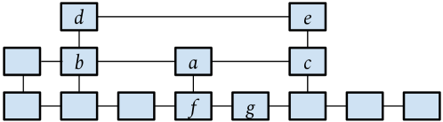
Figure 1: An example skip list over a sequence of eight elements. On the bottom are all the level-$1$ nodes.

For an element $x$ of height $h$, we allocate a node $v_{i}$ for every level $i=1,2,\dots,h$. Each node has four pointers left, right, up, and down. We set $v_{i}\rightarrow\textsc{up}=v_{i+1}$ and $v_{i}\rightarrow\textsc{down}=v_{i-1}$ for each $i$ to connect between levels. We set $v_{i}\rightarrow\textsc{right}$ to the $i$-th node of the next element of height at least $i$ and similarly $v_{i}\rightarrow\textsc{left}$ to the $i$-th node of the previous element of height at least $i$.

Our skip lists support cyclicity, which is to say that our algorithms are valid even if we link the tail and head of a skip list together. Though this is not conventionally done with sequence data structures, we will find it useful for representing Euler tours of graphs in Section 5 since Euler tours are naturally cyclic sequences. We cannot join upon cyclic sequences, but splitting a cyclic sequence at element $x$ corresponds to unraveling it into a linear sequence with its last element being $x$. Figure 2 illustrates joining and splitting on our skip lists.

Definitions. We now introduce definitions that describe the relationship between nodes. Say we have a node $v$ that represents element $x$ at some level $i$. We call $v\rightarrow\textsc{right}$ $v$’s successor. Similarly, $v\rightarrow\textsc{left}$ is its predecessor. We call $v\rightarrow\textsc{up}$ its direct parent and $v\rightarrow\textsc{down}$ its direct child. For example, in Figure 1, consider node $a$. Its predecessor is $b$, its successor is $c$, its direct child is $f$, and it has no direct parent.

The left parent is the level-$(i+1)$ node of the latest element preceding and including $x$ that has height at least $i+1$. The right parent is defined symmetrically. Under this definition, if $v$ has a direct parent, then its left and right parents are both its direct parent. When we refer to $v$’s parent, we refer to its left parent. In Figure 1, $a$’s (left) parent is $d$, and $a$’s right parent is $e$. The (left) ancestors consist of $v$’s parent, $v$’s parent’s parent, and so on, and similarly for $v$’s right ancestors. Thus the ancestors for both $f$ and $g$ in Figure 1 are $a$ and $d$. A child is inverse to a parent, and a descendant is inverse to an ancestor.

The following definitions describe the relationship between the links connecting nodes. The parent of a link between $v$ and its successor is the link between $v$’s parent and its successor. Similarly, the ancestors of the link are links between $v$’s ancestors and their successors. The children of the link are the links between $v$’s children and their successors.

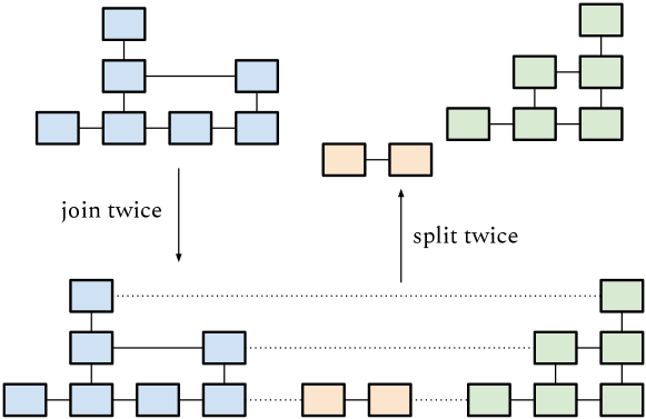
Figure 2: Joins and splits on skip lists.

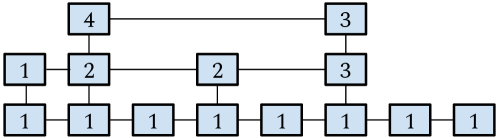
Figure 3: Each node in this skip list is augmented with a size value, summing all the values of its children.

Joins, Splits, and Augmentation on Skip Lists. Recall that in an augmented sequence, we take an associative function $f:D^{2}\to D$ for some domain $D$. Each element in the sequence $A$ is assigned some value from $D$. By storing these values in the bottom level of our skip list and storing partial “sums” at higher levels, we can compute $f$ over contiguous subsequences of $A$ in logarithmic time. For instance, in Figure 3, we assign the value $1$ to every element and choose $f:\mathbb{N}^{2}\to\mathbb{N}$ to be the sum function. For each node $v$, we store the sum of the values of $v$’s children. By looking at $O(\log n)$ nodes, we can then compute the size of the sequence. These augmented values are also easy to maintain as the skip list undergoes joins and splits.

Our skip lists support batch joins, batch splits, batch point updates of augmented values, and batch finding representatives in $O(k\log(1+n/k))$ work in expectation and $O(\log n)$ depth with high probability, where $k$ is the batch size and $n$ is the number of elements in the lists. We analyze efficiency in Appendix D.

This improves on the $\Theta(k\log n)$ expected work bound achieved by conventional sequential joins and splits on augmented skip lists. Intuitively, the reason we can achieve improved work-bounds is that if a node has many updated descendants, our algorithm updates its augmented value only once rather than multiple times.

4.3 Algorithms for unaugmented lists

Algorithm 1 Creates an element with height distributed according to $\operatorname{Geometric}(1-p)$.

1:procedure CreateNode()

2:    allocate $\mathit{node}$

3:    With probability $p$:     

4:         $\mathit{node}\rightarrow\textsc{up}=\textsc{CreateNode}(\hbox{})$

5:         $\mathit{node}\rightarrow\textsc{up}\rightarrow\textsc{down}=\mathit{node}$     

6:    return $\mathit{node}$

We begin by describing unaugmented skip lists. For creating elements in our skip list, we fix a probability $0<p<1$ representing the expected proportion of nodes at a particular level that have a direct parent at the next level. We generate heights of elements by allocating a node and giving each node a direct parent with probability $p$ independently, as seen in Algorithm 1. This is equivalent to drawing heights from a $\operatorname{Geometric}(1-p)$ distribution.

Algorithm 2 Searches for the left parent of the input node. The mirror function SearchRight is defined symmetrically.

1:procedure SearchLeft($\mathit{v}$)

2:    $\mathit{current}=\mathit{v}$

3:    while $\mathit{current}\rightarrow\textsc{up}=\mathit{null}$ do

4:         $\mathit{current}$ = $\mathit{current}\rightarrow\textsc{left}$

5:         if $\mathit{current}=\mathit{null}$ or $\mathit{current}=\mathit{v}$ then

6:             return $\mathit{null}$              

7:    return $\mathit{current}\rightarrow\textsc{up}$

We give pseudocode for Join and Split over unaugmented lists in Algorithms 3 and 4 respectively. To perform a batch of joins, we simply call Join on each join operation in the batch concurrently, and similarly for a batch of splits. As each batch of splits and joins must be run in separate phases, our data structure is phase-concurrent over joins and splits, which is more general than being batch-parallel [42].

Both algorithms employ two simple helper procedures, SearchLeft and SearchRight, for finding the left and right parents of a node. We show SearchLeft in Algorithm 2, and SearchRight is implemented symmetrically. Note that these procedures avoid looping forever on cyclic skip lists.

Algorithm 3 Joins two lists together given their endpoints.

1:procedure Join($\mathit{v}_{L}$, $\mathit{v}_{R}$)

2:    if $\textsc{CAS}(\&\mathit{v}_{L}\rightarrow\textsc{right},\mathit{null},\mathit{v}_{R})$ then

3:         $\mathit{v}_{R}\rightarrow\textsc{left}=\mathit{v}_{L}$

4:         $\mathit{parent}_{L}$ = SearchLeft($v_{L}$)

5:         $\mathit{parent}_{R}$ = SearchRight($v_{R}$)

6:         if $\mathit{parent}_{L}\neq\mathit{null}$ and $\mathit{parent}_{R}\neq\mathit{null}$ then

7:             Join($\mathit{parent}_{L},\mathit{parent}_{R}$)              

Join. Recall that the definition of Join takes a pointer to the last element of one list and a pointer to the first element of a second list and concatenates the first list with the second list. Starting at the bottom level, our algorithm links the given nodes, searches upwards to find parents to link at the next level, and repeats. We set the link with a CAS, and if the CAS is lost, the algorithm quits. This permits only one thread to set a particular link, preventing repeated work.

Theorem 1.

Let $B$ be a set of valid Join inputs. Then calling Join concurrently over the inputs in $B$ gives the same result as joining over the inputs in $B$ sequentially.

Proof.

(Proof sketch) We argue inductively level-by-level that all necessary links are added and no unnecessary links are added. For the base case, at the bottom level, the links we add are exactly those given as input to the algorithm, which are the necessary links to add at that level. For the inductive step, assume that the correct links will be added on level $i$. Consider any link $\ell$ from nodes $v_{L}$ to $v_{R}$ on level $i+1$ that should be added. In order for this to be a link we need to add, there must be a rightward path from $v_{L}$’s direct child to $v_{R}$’s direct child once all links on level $i$ are added. Then consider the last execution of join on level $i$ to add a link on that path by finishing line 3 of Algorithm 3. That execution will have a complete path to find parents $v_{L}$ and $v_{R}$ when searching and thus will find $\ell$ as a link to add. Conversely, any level-$(i+1)$ link from nodes $v_{L}$ to $v_{R}$ found by a join execution was found via a complete path (albeit perhaps temporarily missing some left pointers due to some executions of join completing line 2 but not yet completing line 3) between $v_{L}$’s direct child and $v_{R}$’s direct child, which indicates that this link should be added. We present a formal proof using this idea in Appendix C.1. ∎

Algorithm 4 Separates the input node from its successor.

1:procedure Split($\mathit{v}$)

2:    $\mathit{ngh}=\mathit{v}\rightarrow\textsc{right}$

3:    if $\mathit{ngh}\neq\mathit{null}$ and $\textsc{CAS}(\&\mathit{v}\rightarrow\textsc{right},\mathit{ngh},\mathit{null})$ then

4:         $\mathit{ngh}\rightarrow\textsc{left}=\mathit{null}$

5:         $\mathit{parent}=\textsc{SearchLeft}(v)$

6:         if $\mathit{parent}\neq\mathit{null}$ then

7:             $\textsc{Split}(\mathit{parent})$              

Split. Split takes a pointer to an element and breaks the list right after that element. Similar to join, it cuts the link at the bottom level and then loops in searching upwards to find parent links to remove at higher levels. Like Join, this uses CAS to avoid duplicate work.

Theorem 2.

Let $B$ be a set of elements. Then calling Split concurrently over the elements in $B$ gives the same result as splitting over the elements in $B$ sequentially.

Proof.

(Proof sketch) Like in the proof sketch of Theorem 1, we look at the links that are removed inductively level-by-level. The argument is similar, except that in the inductive step, to see that a link $\ell$ on level $i+1$ from nodes $\mathit{v}_{L}$ to $\mathit{v}_{R}$ that should be removed will indeed be removed by the phase of splits, we note that the leftmost split on the path from $\mathit{v}_{L}\rightarrow\textsc{down}$ to $\mathit{v}_{R}\rightarrow\textsc{down}$ will be able to find parent $\mathit{v}_{L}$ in its SearchLeft call. We present a formal proof using this idea in Appendix C.2. ∎

Finding representative nodes.

Algorithm 5 Finds a representative node of the list that the input node lives in.

1:procedure FindRep($\mathit{v}$)

2:    while $\textsc{SearchRight}(\mathit{v})\not=\mathit{null}$ do

3:         $\mathit{v}=\textsc{SearchRight}(\mathit{v})$     

4:    while $\textsc{SearchLeft}(\mathit{v})\not=\mathit{null}$ do

5:         $\mathit{v}=\textsc{SearchLeft}(\mathit{v})$     

6:    $\mathit{rep}=\mathit{v}$

7:    while true do

8:         if $\mathit{v}\rightarrow\textsc{left}=\mathit{null}$ then $\triangleright$ List is acyclic

9:             return $\mathit{v}$          

10:         $\mathit{v}=\mathit{v}\rightarrow\textsc{left}$

11:         if $\mathit{v}=\mathit{rep}$ then $\triangleright$ List is cyclic

12:             return $\mathit{rep}$          

13:         if $\mathit{v}<\mathit{rep}$ then

14:             $\mathit{rep}=\mathit{v}$              

A simple phase-concurrent implementation of FindRep that takes $O(k\log n)$ expected work for $k$ concurrent calls is to start at the input node and walk to the top level of the list. Then on the top level, for an acyclic list, we return the leftmost node, or for a cyclic list, we return the node with the lowest memory address. This is shown in Algorithm 5.

However, if we are given a batch of $k$ calls up front, we can in fact achieve $O(k\log(1+n/k))$ expected work and $O(\log n)$ depth with high probability. The idea is that each call of FindRep takes some path up the skip list to the top level, and calls whose paths intersect somewhere can be combined at that point to avoid duplicate work. Then the return value gets propagated back down to both original calls. The code would look similar to the code for batch updating augmented values for augmented skip lists (Subsection 4.4) in Algorithm 7. We omit the full details.

4.4 Algorithm for augmented lists

We now describe how to augment our skip lists. In addition to its four pointers, each node is given a value val from some domain $D$ and a boolean needs_update. We provide an associative function $f:D^{2}\to D$ and, for each element in the list, a value from $D$. We assign values to val on nodes at the bottom level and then compute val at higher levels by applying $f$ over nodes’ children. The boolean needs_update is initialized to $\mathit{false}$ and is used to mark nodes whose values need updating.

Algorithm 6 Helper function for BatchUpdateValues that updates the augmented value for $v$ and all its descendants.

1:procedure UpdateTopDown($v$)

2:    $v\rightarrow\textsc{needs\_update}=\mathit{false}$

3:    if $v\rightarrow\textsc{down}=\mathit{null}$ then $\triangleright$ Reached bottom level

4:         return     

5:    $\mathit{current}=v\rightarrow\textsc{down}$

6:    do

7:         if $\mathit{current}\rightarrow\textsc{needs\_update}$ then

8:             spawn $\textsc{UpdateTopDown}(current)$          

9:         $\mathit{current}=\mathit{current}\rightarrow\textsc{right}$

10:    while $\mathit{current}\not=\mathit{null}$ and $\mathit{current}\rightarrow\textsc{up}=\mathit{null}$

11:    sync

12:    $\mathit{sum}=v\rightarrow\textsc{down}\rightarrow\textsc{val}$

13:    $\mathit{current}=v\rightarrow\textsc{down}\rightarrow\textsc{right}$

14:    while $\mathit{current}\not=\mathit{null}$ and $\mathit{current}\rightarrow\textsc{up}=\mathit{null}$ do

15:         $\mathit{sum}=f(\mathit{sum},\mathit{current}\rightarrow\textsc{val})$

16:         $\mathit{current}=\mathit{current}\rightarrow\textsc{right}$     

17:    $v\rightarrow\textsc{val}=\mathit{sum}$

Algorithm 7 Takes a batch of (node, value) pairs, updates each node with its associated value, and updates other affected augmented values stored throughout the list.

1:procedure BatchUpdateValues($\mathopen{}\mathclose{{}\left\{(v_{1},a_{1}),\dots,(v_{k},a_{k})}\right\}$)

2:    $\mathit{top}=\mathopen{}\mathclose{{}\left\{\mathit{null},\mathit{null},\dots,\mathit{null}}\right\}$ $\triangleright$ $k$-length array

3:    for $i\in\mathopen{}\mathclose{{}\left\{1,\dots,k}\right\}$ do in parallel

4:         $v_{i}\rightarrow\textsc{val}=a_{i}$

5:         $\mathit{current}=v_{i}$

6:         while $\textsc{CAS}(\&\mathit{current}\rightarrow\textsc{needs\_update},\mathit{false},\mathit{true})$ do

7:             $\mathit{parent}=\textsc{SearchLeft}(current)$

8:             if $\mathit{parent}=\mathit{null}$ then

9:                 $\mathit{top}[i]=current$

10:                 break              

11:             $\mathit{current}=\mathit{parent}$              

12:    for $i\in\mathopen{}\mathclose{{}\left\{1,\dots,k}\right\}$ do in parallel

13:         if $\mathit{top}[i]\not=\mathit{null}$ then

14:             $\textsc{UpdateTopDown}(\mathit{top}[i])$              

We give the main algorithm BatchUpdateValues for batch augmented value update in Algorithm 7. This takes a set of nodes at the bottom level along with values to give to the associated elements. For each node in the set, we start by updating its value (line 5). Then each of its ancestors have values that need updating, so we walk up its ancestors, CASing on each ancestor’s needs_update variable (line 6). If an execution loses a CAS, then it may quit because some other execution will take care of all the node’s ancestors.

Now over all the input nodes that won all CASes on their ancestors, we know the union of their topmost ancestors’ descendants contain all the input nodes. By calling the helper function UpdateTopDown (Algorithm 6) on every such topmost ancestor in lines 12–14, we traverse back down and update these descendants’ augmented values. Given a node, this helper function calls itself recursively on all the node’s children $c$ who need an update as indicated by $c\rightarrow\textsc{needs\_update}$ (lines 5–10). Then, after all the childrens’ values are updated, we may update the original node’s value (lines 11–17).

Algorithm 8 Batch join for augmented skip lists.

1:procedure BatchJoin($\mathopen{}\mathclose{{}\left\{(l_{1},r_{1}),(l_{2},r_{2}),\dots,(l_{k},r_{k})}\right\}$)

2:    for $i\in\mathopen{}\mathclose{{}\left\{1,\dots,k}\right\}$ do in parallel

3:         $\textsc{Join}(l_{i},r_{i})$     

4:    $\textsc{BatchUpdateValues}(\mathopen{}\mathclose{{}\left\{(l_{1},l_{1}\rightarrow\textsc{val}),\dots,(l_{k},l_{k}\rightarrow\textsc{val})}\right\})$

Algorithm 9 Batch split for augmented skip lists.

1:procedure BatchSplit($\mathopen{}\mathclose{{}\left\{v_{1},v_{2},\dots,v_{k}}\right\}$)

2:    for $i\in\mathopen{}\mathclose{{}\left\{1,\dots,k}\right\}$ do in parallel

3:         $\textsc{Split}(v_{i})$     

4:    $\textsc{BatchUpdateValues}(\mathopen{}\mathclose{{}\left\{(v_{1},v_{1}\rightarrow\textsc{val}),\dots,(v_{k},v_{k}\rightarrow\textsc{val})}\right\})$

With this algorithm for batch augmented value update, batch joins (Algorithm 8) and batch splits (Algorithm 9) are simple. We first perform all the joins or splits. Then we batch update on the nodes we joined or split on. We keep all the values on the bottom level the same, but the update fixes all the values on the higher levels that are changed by adding or removing links.

Algorithm 10 Query for the augmented value over the subsequence between $v_{L}$ and $v_{R}$ inclusive. Here we let $f(\mathit{none},x)=x$ for all $x\in D$.

1:procedure QueryValue($v_{L}$, $v_{R}$)

2:    $\mathit{sum}_{L}=\mathit{none}$

3:    $\mathit{sum}_{R}=v_{R}\rightarrow\textsc{val}$

4:    while $v_{L}\not=v_{R}$ do

5:         while $v_{L}\rightarrow\textsc{up}\not=\mathit{null}$ and $v_{R}\rightarrow\textsc{up}\not=\mathit{null}$ do

6:             $v_{L}=v_{L}\rightarrow\textsc{up}$

7:             $v_{R}=v_{R}\rightarrow\textsc{up}$          

8:         if $v_{L}\rightarrow\textsc{up}=\mathit{null}$ then

9:             $\mathit{sum}_{L}=f(\mathit{sum}_{L},v_{L}\rightarrow\textsc{val})$

10:             $v_{L}=v_{L}\rightarrow\textsc{right}$

11:         else

12:             $v_{R}=v_{R}\rightarrow\textsc{left}$

13:             $\mathit{sum}_{R}=f(v_{R}\rightarrow\textsc{val},\mathit{sum}_{R})$              return $f(\mathit{sum}_{L},\mathit{sum}_{R})$

A batch of $k$ queries for the augmented values over contiguous subsequences of lists can be processed in $O(k\log n)$ expected work and $O(\log n)$ depth with high probability by simply performing each query with Algorithm 10 in parallel at $O(\log n)$ expected work per query.

4.5 Implementation

We provide details about our skip list implementations in Appendix B.1.

5 Batch-Parallel Euler Tour Trees

In this section we present batch-parallel Euler tour trees, a solution to the batch-parallel dynamic trees problem. In order to ease exposition, we first present a batch-parallel interface for the dynamic trees problem.

Batch-Parallel Dynamic Trees Interface. A solution to the batch-parallel dynamic trees problem supports representing a forest as it undergoes batches of links, cuts, and connectivity queries. Links link two trees in the forest. Cuts delete an edge from the forest and break one tree into two trees. Connectivity queries take two vertices in the forest and return whether they are connected (that is, whether they are in the same tree). We now give a formal description of the interface. The data structure maintains a graph $G=(E,V)$, which is assumed to be a forest under the following operations:

• $\textsc{BatchLink}(\mathopen{}\mathclose{{}\left\{\mathopen{}\mathclose{{}\left\{u_{1},v_{1}}\right\},\ldots,\mathopen{}\mathclose{{}\left\{u_{k},v_{k}}\right\}}\right\})$ takes an array of edges and adds them to the graph $G$. The input edges must not create a cycle in $G$.

• $\textsc{BatchCut}(\mathopen{}\mathclose{{}\left\{\mathopen{}\mathclose{{}\left\{u_{1},v_{1}}\right\},\ldots,\mathopen{}\mathclose{{}\left\{u_{k},v_{k}}\right\}}\right\})$ takes an array of edges and removes them from the graph $G$.

• $\textsc{BatchConnected}(\mathopen{}\mathclose{{}\left\{\mathopen{}\mathclose{{}\left\{u_{1},v_{1}}\right\},\ldots,\mathopen{}\mathclose{{}\left\{u_{k},v_{k}}\right\}}\right\})$ takes an array of tuples representing queries. The output is an array where the $i$-th entry returns whether vertices $u_{i}$ and $v_{i}$ are connected by a path in $G$.

We also support augmenting the trees with an associative and commutative function $f:D^{2}\to D$ with values from $D$ assigned to vertices and edges of the forest. The goal of augmentation is to compute $f$ over subtrees of the represented forest. Note that we assume that the function is commutative in order to allow implementations to not maintain any specific order over each vertex’s children. The interface supports batch updates over vertices and edges. The primitives are similar to the batch updates of values for augmented skip lists, so we elide the details. The interface for subtree queries is different, and we present it below:

• $\textsc{BatchSubtree}(\mathopen{}\mathclose{{}\left\{(u_{1},p_{1}),\ldots,(u_{k},p_{k})}\right\})$ takes an array of tuples, where the $i$-th tuple contains a vertex $u_{i}$ and its parent $p_{i}$ in the tree. It returns an array where the $i$-th entry contains the value of $f$ summed over $u_{i}$’s subtree relative to its parent $p_{i}$ in $G$. Note that because the represented trees are unrooted, we require providing the parent $p_{i}$ in order to determine the intended subtree for $u_{i}$.

(Some dynamic trees data structures allow queries for augmented values summed over paths rather than subtrees in the represented forest, but Euler tour trees do not.)

Euler Tour Trees. We focus on a variant of Euler tour trees presented by Tarjan [50]. To represent a tree as an Euler tour tree, replace each edge $\mathopen{}\mathclose{{}\left\{u,v}\right\}$ with two directed edges $(u,v)$ and $(v,u)$ and add a loop $(v,v)$ to each vertex $v$, as shown in Figure 4. This construction produces a connected graph in which each vertex has equal indegree and outdegree, and therefore the graph admits an Euler tour. We represent the tree as any of its Euler tours.

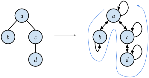
Figure 4: We take the tree on the left and transform it so that we get the following Euler tour of edges: $(a,b)$ $(b,b)$ $(b,a)$ $(a,c)$ $(c,d)$ $(d,d)$ $(d,c)$ $(c,c)$ $(c,a)$ $(a,a)$.

Now linking two trees corresponds to splicing their Euler tours together, and cutting a tree corresponds to cutting out part of its Euler tour. Each of these operations reduces to a few joins and splits on the tours. We may also answer whether two vertices $u$ and $v$ are connected by asking whether their loops, $(u,u)$ and $(v,v)$, reside in the same tour. Moreover, because a subtree appears as a contiguous section of an Euler tour, we can efficiently compute information about subtrees if we can efficiently compute information about contiguous sections of tours.

Traditionally, Euler tour trees store an Euler tour by breaking it into a sequence at an arbitrary location and then placing the sequence in a balanced binary tree. We instead store Euler tours as cycles using our skip lists from Section 4. Because skip lists are easy to join and split in parallel, we can process batches of links and cuts on Euler tour trees efficiently.

We show that for a batch of $k$ joins, $k$ splits, or $k$ connectivity queries over an $n$-vertex forest, we can achieve $O(k\log(1+n/k))$ expected work and $O(\log n)$ depth with high probability. If we build our Euler tour trees over augmented skip lists, we can also answer subtree queries efficiently.

5.1 Description

Our Euler tour trees crucially rely on our parallel skip lists to represent Euler tours. Since a graph of $n$ vertices has Euler tours whose lengths sum to $O(n)$, the skip lists hold $O(n)$ elements. Thus a batch of $k$ joins or splits on the Euler tours takes $O(k\log(1+n/k))$ expected work and $O(\log n)$ depth with high probability.

Construction. For clarity, we describe our Euler tour trees using the phase-concurrent unaugmented skip lists given in Section 4. However, it is easy to organize the joins and splits into batches so as to match the augmented skip list interface seen in Subsection 4.4. We also treat our dictionary data structure as phase-concurrent for clarity, but again, this is easy to circumvent.

We add fields twin and mark to each skip list element. For an element representing a directed edge $(u,v)$, twin is a pointer to the element representing the directed edge $(v,u)$ in the opposite direction. We initialize the field mark to $\mathit{false}$ and use it during splitting to mark elements that will be removed.

Algorithm 11 Euler tour tree data structure initialization.

1:procedure Initialize($n$)

2:    $\mathit{verts}=\mathopen{}\mathclose{{}\left\{}\right\}$ $\triangleright$ $n$-length array

3:    for $i\in\mathopen{}\mathclose{{}\left\{1,\dots,n}\right\}$ do in parallel

4:         $\mathit{verts[i]}=\textsc{CreateNode}(\hbox{})$

5:         Join($\mathit{verts}[i],\mathit{verts}[i]$)     

6:    $\mathit{edges}=\textsc{dict}(\hbox{})$ $\triangleright$ empty dictionary

7:    $\mathit{successors}=\mathopen{}\mathclose{{}\left\{}\right\}$ $\triangleright$ $n$-length array

At initialization (Algorithm 11), the represented graph is an $n$-vertex forest with no edges, and we assume the vertices are labeled with integers $1,2,\dots,n$. We create an $n$-length array $\mathit{verts}$ such that $\mathit{verts}[i]$ stores a pointer to the skip list element representing the loop edge $(i,i)$. As such, in parallel, for $i=1,\dots,n$, we create a skip list element, assign it to $\mathit{verts}[i]$, and join it to itself to form a singleton cycle. These cycles are the Euler tours in an empty graph. We also keep a dictionary $\mathit{edges}$ that maps edges $(u,v)$ with $u\not=v$ to corresponding skip list elements. Lastly, we create an array $\mathit{successors}$ that will be used as scratch space for batch linking.

Connectivity queries. To check whether two vertices are connected, we simply check whether they live in the same Euler tour by comparing the representatives of their tours’ skip lists. The complexity of this can be made $O(k\log(1+n/k))$ expected work and $O(\log n)$ depth with high probability using an efficient BatchFindRep algorithm.

Algorithm 12 Add a batch of edges to Euler tour tree.

1:procedure BatchLink($\mathopen{}\mathclose{{}\left\{\mathopen{}\mathclose{{}\left\{u_{1},v_{1}}\right\},\mathopen{}\mathclose{{}\left\{u_{2},v_{2}}\right\},\dots,\mathopen{}\mathclose{{}\left\{u_{k},v_{k}}\right\}}\right\}$)

2:    $\triangleright$ Adding input edges must not create a cycle in graph

3:    $\triangleright$ Create nodes representing new edges

4:    for $i\in\mathopen{}\mathclose{{}\left\{1,\dots,k}\right\}$ do in parallel

5:         $\mathit{uv}=\textsc{CreateNode}(\hbox{})$

6:         $\mathit{vu}=\textsc{CreateNode}(\hbox{})$

7:         $\mathit{uv}\rightarrow\textsc{twin}=\mathit{vu}$

8:         $\mathit{vu}\rightarrow\textsc{twin}=\mathit{uv}$

9:         $\mathit{edges}[(u_{i},v_{i})]=uv$

10:         $\mathit{edges}[(v_{i},u_{i})]=vu$     

11:    $\triangleright$ Cut at locations at which we splice in other tours

12:    for $i\in\mathopen{}\mathclose{{}\left\{1,\dots,k}\right\}$ do in parallel

13:         for $w\in\mathopen{}\mathclose{{}\left\{u_{i},v_{i}}\right\}$ do

14:             $\mathit{w\_node}=\mathit{verts}[w]$

15:             $\mathit{w\_succ}=\mathit{w\_node}\rightarrow\textsc{right}$

16:             if $\mathit{w\_succ}\not=\mathit{null}$ then

17:                 $\triangleright$ benign race; this assignment and split are idempotent

18:                 $\mathit{successors}[w]=\mathit{w\_succ}$

19:                 Split($\mathit{w\_node}$)                           

20:    $\mathit{sorted\_edges}=\newline \makebox[27.00005pt]{}\textsc{Semisort}(\mathopen{}\mathclose{{}\left\{(u_{1},v_{1}),(v_{1},u_{1}),\dots,(u_{k},v_{k}),(v_{k},u_{k})}\right\})$

21:    $\triangleright$ Join together tours with new edge nodes in between

22:    for $i\in\mathopen{}\mathclose{{}\left\{1,\dots,2k}\right\}$ do in parallel

23:         $(\mathit{u},\mathit{v})=\mathit{sorted\_edges}[i]$

24:         $(\mathit{u\_prev},\mathit{v\_prev})=\mathit{sorted\_edges}[i-1]$

25:         $(\mathit{u\_next},\mathit{v\_next})=\mathit{sorted\_edges}[i+1]$

26:         if $i=1$ or $u\not=u\_prev$ then

27:             Join($(\mathit{verts}[\mathit{u}],\mathit{edges}[(\mathit{u},\mathit{v})])$)          

28:         if $i=2k$ or $\mathit{u}\not=\mathit{u\_next}$ then

29:             Join($(\mathit{edges}[(\mathit{v},\mathit{u})],\mathit{successors}[\mathit{u}])$)

30:         else

31:             Join($(\mathit{edges}[(\mathit{v},\mathit{u})],\mathit{edges}[(\mathit{u\_next},\mathit{v\_next})])$)              

Batch Link. Algorithm 12 shows our algorithm for adding a batch of edges. The algorithm takes an array of edges $A$ to add as input. We assume that adding the input edges preserves acyclity.

To add a single edge $\mathopen{}\mathclose{{}\left\{u,v}\right\}$ sequentially, we can find locations where $u$ and $v$ appear in their tours by looking up $\mathit{verts}[u]$ and $\mathit{verts}[v]$. We split on those locations and join the resulting cut up tours back together with new nodes representing $(u,v)$ and $(v,u)$ in between. If we want to add several edges in parallel, we need to be careful when inserting edges that are incident to the same vertex and thus attempt to join on the same location.

With that in mind, we proceed to describe our algorithm. In lines 3-10, for each input edge $\mathopen{}\mathclose{{}\left\{u,v}\right\}$, we allocate new list elements representing directed edges $(u,v)$ and $(v,u)$. Then, in lines 11-19, for each vertex $u$ that appears in the input, we split $u$’s list at $\mathit{verts}[u]$ as a location to splice in other tours. We also save the successor of $\mathit{verts}[u]$ in $\mathit{successors}[u]$ so that we can join everything back together at the end.

For each vertex $u$, say that the input tells us that we want to newly connect $u$ to vertices $w_{1},w_{2},\dots,w_{k}$. Then we join together the nodes representing $(u,u)$ to $(u,w_{1})$, $(w_{i},u)$ to $(u,w_{i+1})$ for $1\leq i<k$, and $(w_{k},u)$ to what was the successor to $(u,u)$ before splitting. In our code, we arrange this in lines 20-31 by semisorting the input to collect together all edges incident on a vertex. The ordering of $w_{1},w_{2},\dots,w_{k}$ is unimportant, only corresponding to the order in which they appear after $u$ in the Euler tour.

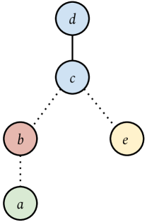
Figure 5: An example graph for illustrating batch linking . The dashed edges $\mathopen{}\mathclose{{}\left\{a,b}\right\},\mathopen{}\mathclose{{}\left\{b,c}\right\},\mathopen{}\mathclose{{}\left\{c,e}\right\}$ are new edges to add in a batch, whereas the solid edge is an already existing edge.

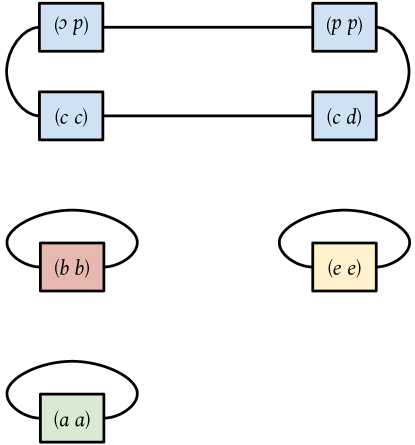
Figure 6: We represent the graph from Figure 5 prior to adding the dashed edges with Euler tours stored in cyclic linked lists.

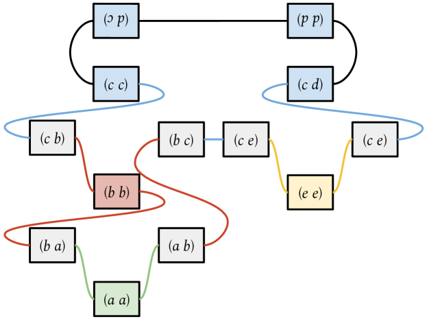
Figure 7: After adding the dashed edges in figure 5, the Euler tour stored in a linked list may look like this. In this figure, we color links in the list the same colors as the nodes “responsible” for adding those links in through calls to Join.

As an example of the desired result from a batch link, consider the graph in Figure 5 on which we wish to perform a batch link with input $\mathopen{}\mathclose{{}\left\{\mathopen{}\mathclose{{}\left\{a,b}\right\},\mathopen{}\mathclose{{}\left\{b,c}\right\},\mathopen{}\mathclose{{}\left\{c,e}\right\}}\right\}$. Prior to the batch link, the Euler tour may look like Figure 6, and after the batch link, the Euler tour may look like Figure 7. Let us focus on what happens to the list containing vertex $c$. After allocating the new nodes representing the new edges to add, we split node $(c,c)$ from its successor $(c,d)$. We want to add edges connecting $c$ to $b$ and to $e$. As such, we perform joins adding links from nodes $(c,c)$ to $(c,b)$, $(b,c)$ to $(c,e)$, and $(e,c)$ to $(c,d)$. These new links correspond to the blue links in figure 7. Doing this over all vertices provides all the joins needed to form an Euler tour over the whole graph.

Using our skip lists and an efficient semisort [20], we see that the work is $O(k\log(1+n/k))$ in expectation, and the depth is $O(\log n)$ with high probability.

Algorithm 13 Computes locations at which to join for batch cut.

1:procedure GetNextUnmarked($\mathit{elements}=\mathopen{}\mathclose{{}\left\{z_{1},z_{2},\dots,z_{k}}\right\}$)

2:    $\triangleright$ Input is a set of skip list elements

3:    for $i\in\mathopen{}\mathclose{{}\left\{1,\dots,k}\right\}$ do in parallel

4:         $\mathit{next}=z_{i}\rightarrow\textsc{twin}\rightarrow\textsc{right}$

5:         if $\mathit{next}\rightarrow\textsc{mark}$ then

6:             $z_{i}\rightarrow\textsc{next\_edge}=\mathit{next}$

7:         else

8:             $z_{i}\rightarrow\textsc{next\_edge}=\mathit{null}$              

9:    $\triangleright$ Use list tail-finding on the linked lists induced by next_edge pointers. Get an array $\mathit{last\_marked}$ such that $\mathit{last\_marked}[i]$ points to the last node in $z_{i}$’s linked list.

10:    $\mathit{last\_marked}=\textsc{ListTailFind}(\mathit{elements})$

11:    $\mathit{result}=\mathopen{}\mathclose{{}\left\{}\right\}$ $\triangleright$ $k$-length array

12:    for $i\in\mathopen{}\mathclose{{}\left\{1,\dots,k}\right\}$ do in parallel

13:         $\mathit{result}[i]=\mathit{last\_marked}[i]\rightarrow\textsc{twin}\rightarrow\textsc{right}$     

14:    return $\mathit{result}$

Algorithm 14 Remove a batch of edges from Euler tour tree.

1:procedure BatchCut($\mathopen{}\mathclose{{}\left\{\mathopen{}\mathclose{{}\left\{u_{1},v_{1}}\right\},\mathopen{}\mathclose{{}\left\{u_{2},v_{2}}\right\},\dots,\mathopen{}\mathclose{{}\left\{u_{k},v_{k}}\right\}}\right\}$)

2:    $\triangleright$ Input edges must be in graph and must have no duplicates.

3:    $\mathit{directed\_edges}=\mathopen{}\mathclose{{}\left\{}\right\}$ $\triangleright$ $2k$-length array

4:    for $i\in\mathopen{}\mathclose{{}\left\{1,\ldots,k}\right\}$ do in parallel

5:         $\mathit{directed\_edges}[2i-1]=\mathit{edges}[(u_{i},v_{i})]$

6:         $\mathit{directed\_edges}[2i]=\mathit{edges}[(v_{i},u_{i})]$     

7:    for $i\in\mathopen{}\mathclose{{}\left\{1,\ldots,k}\right\}$ do in parallel

8:         $\mathit{edges}\rightarrow\textsc{RemoveFromDict}((u_{i},v_{i}))$

9:         $\mathit{edges}\rightarrow\textsc{RemoveFromDict}((v_{i},u_{i}))$     

10:    $\mathit{join\_lefts}=\mathopen{}\mathclose{{}\left\{}\right\}$ $\triangleright$ $2k$-length array

11:    for $i\in\mathopen{}\mathclose{{}\left\{1,\ldots,2k}\right\}$ do in parallel

12:         $\mathit{join\_lefts}[i]=\mathit{directed\_edges}[i]\rightarrow\textsc{left}$

13:         $\mathit{directed\_edges}[i]\rightarrow\textsc{mark}=\mathit{true}$     

14:    $\mathit{join\_rights}=\textsc{GetNextUnmarked}(\mathit{directed\_edges})$

15:    $\triangleright$ Cut edges out of tour

16:    for $i\in\mathopen{}\mathclose{{}\left\{1,\ldots,2k}\right\}$ do in parallel

17:         Split($\mathit{directed\_edges}[i]$)

18:         $\mathit{pred}=\mathit{directed\_edges}[i]\rightarrow\textsc{Left}$

19:         if $\mathit{pred}\not=\mathit{null}$ then

20:             $\textsc{Split}(\mathit{pred})$              

21:    $\triangleright$ Join tours back together

22:    for $i\in\mathopen{}\mathclose{{}\left\{1,\ldots,2k}\right\}$ do in parallel

23:         if not $\mathit{join\_lefts}[i]\rightarrow\textsc{mark}$ then

24:             Join($\mathit{join\_lefts}[i],\mathit{join\_rights}[i]$)              

25:    for $i\in\mathopen{}\mathclose{{}\left\{1,\ldots,2k}\right\}$ do in parallel

26:         DeleteNode($\mathit{directed\_edges}[i]$)     

Batch Cut. Algorithm 14 describes how to remove a batch of edges. Our algorithm assumes that each edge exists in the forest and that there are no duplicates.

Cutting a single edge is simple. If we cut an edge $\mathopen{}\mathclose{{}\left\{u,v}\right\}$, we split before and after $(u,v)$ and $(v,u)$ in the tour and join their neighbors together appropriately. However, as with batch linking, the task gets more difficult if we want to cut many edges out of a single node, because those neighbors that we want to join together may themselves be split off.

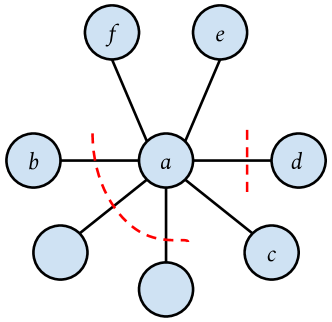
Figure 8: Batch cutting four edges. If we take an Euler tour counter-clockwise around this graph, this batch cuts may require us to join $(f,a)$ to $(a,c)$ in the tour.

As an example, consider the graph in Figure 8 in which we remove four edges. If our tour on the graph goes counter-clockwise around the diagram, then we may need to join $(c,a)$ to $(a,e)$ in the tour as a result of cutting $\mathopen{}\mathclose{{}\left\{a,d}\right\}$ and join $(f,a)$ all the way around to $(a,c)$ as a result of the three contiguous cuts. How do we identify that we need to join $(f,a)$ to $(a,c)$? We could mark edges that are going to be cut, then start from $(f,a)$ and walk along “adjacent” edges incident to $a$ using the twin pointers until we reach an edge that will not be cut. Then we would know to join $(f,a)$ to that edge. However, the search for an unmarked edge will have poor depth if lots of edges will be cut.

To achieve low depth in this step, we use list tail-finding. Consider the linked lists induced by having each edge point at its adjacent edge if it is marked. Note that each linked list must terminate because traversing adjacent edges will eventually reach a loop edge of the form $(v,v)$, which will certainly be unmarked. Then running list tail-finding on these linked lists finds for every edge the next unmarked edge as desired.

In Algorithm 14, we first fetch all the skip list nodes corresponding to the edges in lines 2-6. Then we invoke Algorithm 13 on line 14, which performs the list tail-finding described above. We cut out all the input edges on lines 15-20 and rejoin all the tours together on lines 21-24. In total these steps take $O(k\log(1+n/k))$ expected work and $O(\log n)$ depth with high probability.

Augmentation. We build our augmented Euler tour trees over the concurrent augmented skip lists from Subsection 4.4 and achieve the same efficiency bounds. Recall that we have an associative and commutative function $f:D^{2}\to D$ and assign values from $D$ to vertices and edges of the forest. The goal is to compute $f$ over subtrees of the represented forest.

Say we want to compute $f$ over a vertex $v$’s subtree relative to $v$’s parent in the tree, $p$. Then if we look up the skip list elements corresponding to $(p,v)$ and $(v,p)$ in $\mathit{edges}$, the value of $f$ over $v$’s subtree is the result of applying $f$ on the subsequence between $(p,v)$ and $(v,p)$. This may be done by calling BatchQueryValue with the elements corresponding to $(p,v)$ and $(v,p)$ in the underlying augmented skip list. The complexity for $k$ such queries is $O(k\log n)$ expected work and $O(\log n)$ depth with high probability.

5.2 Implementation

We provide details about our implementation of Euler tour trees in Appendix B.2.

6 Experiments

We run our experiments on a 72-core Dell PowerEdge R930 (with two-way hyper-threading) with 4 $\times$ 2.4GHz Intel 18-core E7-8867 v4 Xeon processors (with a 4800MHz bus and 45MB L3 cache) and 1TB of main memory. Our programs use Cilk Plus to express parallelism and are compiled with the g++ compiler (version 5.5.0). When running in parallel, we use the command numactl -i all to evenly distribute the allocated memory among the processors. On our figures, a thread count of 72(h) denotes using all $72$ cores with hyper-threading, i.e. using 144 threads.

6.1 Unaugmented Skip Lists

We evaluate the performance of our skip lists (with the probability of a node having a direct parent set to $p=1/2$) by comparing them against other sequence data structures. In particular, we compare against sequential skip lists, which are the same as our skip lists except that they do not use CAS to set pointers. In addition, for an element of height $h$, they allocate an array of exactly length $h$ for holding pointers rather than an array of length $O(h)$ as our parallel skip list implementation does (see Appendix B.1). We also implemented splay trees [47] and treaps [7].

So that we can compare against another parallel data structure, we implement parallel batch join and batch split operations on treaps. To batch join, we first ignore a constant fraction of the joins. If we imagine each join from treap $T$ to treap $S$ as a pointer from $T$ to $S$, we get lists on the treaps. No list can be very long because of the ignored joins. We get parallelism by processing each list independently. If we store extra information on the treap nodes, we can walk along a list and perform its joins sequentially. Then we recursively process the previously ignored joins. For batch split, we semisort the splits keyed on the root of the treap to be split. This lets us find all splits that act on a particular treap. We process each treap independently. When performing multiple splits on a treap, we get parallelism by divide and conquer—we perform a random split and recursively split the resulting two treaps in parallel. The randomized efficiency bounds are $O(k\log n)$ work for batch join, $O(k\log n\log k)$ work for batch split, and $O(\log n\log k)$ depth for both. In the future, we would like to further compare our skip lists against other parallel data structures, such as the $(a,b)$-trees of Akhremtsev and Sanders [3].

For an experiment, we take $n=10^{8}$ elements and fix a batch size $k$. We set up a trial by joining all the elements in a chain, and then we time how long it takes to split and rejoin the sequence at $k$ pseudorandomly sampled locations. We report the median time over three trials. As an artifact of this setup, the splay tree has an advantage on joining small batches after splitting due to how splay trees exploit locality.

Data structure	Batch size $k$	Operation	Number of threads
			1	2	4	8	16	32	64	72	72(h)
Concurrent skip list	$10^{4}$	join	.0301	.0165	.0101	.00632	.00298	.00166	.000937	.000839	.000530
		split	.0331	.0173	.0113	.00579	.00298	.00154	.000865	.000775	.000542
	$10^{7}$	join	12.6	6.43	4.07	2.05	1.03	.528	.279	.267	.156
		split	10.4	5.34	3.34	1.86	.869	.426	.228	.214	.122

Table 1: Running time (in seconds) of our concurrent skip lists with $n=10^{8}$.

Figure 9: Speedup of our concurrent skip lists with $n=10^{8}$.

Data structure	Operation	Batch size $k$
		$10^{2}$	$10^{3}$	$10^{4}$	$10^{5}$	$10^{6}$	$10^{7}$	$10^{8}-1$
Concurrent skip list (72(h))	join	.0000629	.000122	.000595	.00461	.0347	.161	.684
	split	.0000629	.000132	.000660	.00363	.0254	.131	.559
Concurrent skip list (1)	join	.000300	.00260	.0295	.376	2.44	12.8	54.7
	split	.000383	.00355	.0325	.281	1.90	10.6	47.6
Sequential skip list	join	.000324	.00265	.0275	.362	2.26	11.7	44.9
	split	.000396	.00359	.0319	.272	1.80	9.87	45.0
Parallel treap (72(h))	join	.000227	.000758	.00141	.00475	.0250	.112	.447
	split	.000335	.00186	.00521	.0277	.265	2.54	22.8
Sequential treap	join	.0000989	.00104	.00712	.183	1.23	6.86	25.2
	split	.000231	.00213	.0189	.168	1.30	7.69	33.5
Splay tree	join	.0000689	.000688	.00575	.106	1.09	7.79	32.1
	split	.000329	.00284	.0255	.215	1.63	9.21	36.3

Table 2: Running time (in seconds) of sequence data structures with $n=10^{8}$ and varying batch size.

(a) Join

(b) Split

Figure 10: Running time of sequence data structures operations with varying batch size.

Table 1 and Figure 9 illustrate that our skip list implementation running on $72$ cores with hyper-threading demonstrates over $80\times$ speedup relative to the implementation running on a single thread for $k=10^{7}$ and over $55\times$ speedup for $k=10^{4}$. We compare our skip list to our other sequence data structures in Table 2 and Figure 10 . Our implementation of parallel batch join on treaps is $1.4\times$ faster than our batch join on skip lists on the largest batch sizes, but, as seen in Figure 10, the parallel batch split on treaps is much slower due to lots of overhead work. Moreover, through parallelism, our data structure is significantly faster than all the sequential algorithms at all batch sizes. When used sequentially, our data structure behaves similarly to a traditional sequential skip list, suggesting that using CAS does not significantly degrade the performance of a skip list.

6.2 Augmented Skip Lists

We compare the performance of our batch-parallel augmented skip lists against a sequential augmented skip list. Besides not using CAS, the sequential skip list updates augmented values after every join and split. This achieves only an $O(k\log n)$ work bound for $k$ operations. Our experiment is the same as in Subsection 6.1.

Data structure	Batch size $k$	Operation	Number of threads
			1	2	4	8	16	32	64	72	72(h)
Parallel skip list	$10^{4}$	join	.0908	.0457	.0251	.0164	.00871	.00487	.00292	.00282	.00227
		split	.0546	.0283	.0195	.0134	.00561	.00306	.00177	.00164	.00113
	$10^{7}$	join	24.9	12.7	9.39	4.41	2.10	1.09	.614	.61	.374
		split	19.7	10.1	7.49	3.48	1.61	.810	.422	.398	.253

Table 3: Running time (in seconds) of our parallel augmented skip lists with $n=10^{8}$.

Figure 11: Speedup of our parallel augmented skip lists with $n=10^{8}$.

Data structure	Operation	Batch size $k$
		$10^{2}$	$10^{3}$	$10^{4}$	$10^{5}$	$10^{6}$	$10^{7}$	$10^{8}-1$
Parallel skip list (72(h))	join	.000301	.000559	.00205	.0131	.0825	.357	1.35
	split	.000152	.000312	.00117	.00727	.0450	.229	1.03
Parallel skip list (1)	join	.000823	.00697	.0893	1.04	5.73	25.5	102
	split	.00079	.00625	.0514	.557	3.74	20.2	83.7
Sequential skip list	join	.000716	.00575	.0764	.724	4.79	27.5	131
	split	.000712	.00647	.0583	.489	3.35	19.6	93.3

Table 4: Running time (in seconds) of augmented skip lists with $n=10^{8}$ on random batches of varying size.

(a) Join

(b) Split

Figure 12: Running time of augmented sequence data structure operations with $n=10^{8}$ on random batches of varying size.

Table 3 and Figure 11 show that when running our augmented skip list with a random batch of size $k=10^{7}$ on $72$ cores with hyper-threading, we see a speedup of $67\times$ for joins and $78\times$ for splits. For $k=10^{4}$, we found a speedup of $33\times$ for joins and $48\times$ for splits. The running times are a factor of two worse than the times for the unaugmented skip list of Subsection 6.1, which is expected due to the extra passes through the skip list to update augmented values. Moreover, the batch-parallel skip list hugely outperforms single-threaded skip lists on all tested batch sizes, as seen in Table 4 and Figure 12.

Data structure	Operation	Batch size $k$
		$10^{2}$	$10^{3}$	$10^{4}$	$10^{5}$	$10^{6}$	$10^{7}$	$10^{8}-1$
Parallel skip list (72(h))	split	.000111	.000192	.000272	.000596	.00281	.0259	.252
Parallel skip list (1)	split	.0000350	.000148	.00119	.0115	.119	1.20	11.9
Sequential skip list	split	.000296	.00258	.0219	.210	2.11	21.5	205

Table 5: Running time (in seconds) of splitting augmented skip lists with $n=10^{8}$ as batch size varies with splits taking single elements off the end of the list. This is a difficult test case for standard augmented skip lists.

Figure 13: Running time of splitting augmented skip lists with $n=10^{8}$ as batch size varies with splits taking off single elements off the end of the list.

To more prominently display the work savings that batching provides, we try a different test case in which a batch of $k$ splits, rather than being chosen at random, consists of splitting at the last $k$ elements of the sequence in right-to-left order. This is particularly bad for the sequential skip list because after every split, it walks to the top of the skip list to update augmented values. In comparison, when processing the splits as a batch, we update the augmented values in only one pass. Table 5 and Figure 13 show that, as expected, even on a single thread, our skip list is significantly faster than the standard sequential one in this adversarial experiment.

6.3 Euler Tour Trees

We compare against sequential dynamic trees data structures. Using the sequential skip list and splay trees from Subsection 6.1, we build traditional Euler tour trees. We also compare to ST-trees built on splay trees [46, 47]. They achieve $O(\log n)$ amortized work links and cuts. Though conceptually more complicated than Euler tour trees, ST-trees are a more streamlined data structure that do not require allocation beyond initialization and do not require dictionary lookups. We wrote all of these implementations. In future work, we would like to compare against parallel data structures such as that of Acar et al. [1]

Because one of the important uses of Euler tour trees is to answer connectivity queries, we also compare with statically computing the connected components of the graph. We use the work-efficient parallel connectivity algorithm designed and implemented by Shun et al. [44]. We optimistically measure the execution time of the implementation based only on the execution time of the connectivity algorithm; we do not include the time taken to maintain the graph itself, which is non-trivial because the adjacency array graph representation used in their implementation does not support edge insertion or deletion easily.

For our experiment, we fix a tree. We set up a trial by adding all the edges of the tree in pseudorandom order to our data stucture. Then we time how long it takes to cut and relink the forest at $k$ pseudorandomly sampled edges. We report median times over three trials. Again, note that our experimental setup may give the splay tree data structures an advantage on linking small batches after cutting due to how splay trees exploit locality. We experimented on three trees, all with $n=10^{7}$ vertices: a path graph, a star graph, and a random recursive tree. To form a random recursive tree over $n$ vertices, for each $1<i\leq n$, draw $j$ uniformly at random from $\mathopen{}\mathclose{{}\left\{1,2,\ldots,i-1}\right\}$ and add the edge $\mathopen{}\mathclose{{}\left\{j,i}\right\}$.

Data structure	Graph	Batch size $k$	Operation	Number of threads
				1	2	4	8	16	32	64	72	72(h)
Parallel ETT	Path graph	$10^{4}$	link	.175	.109	.0559	.0172	.00988	.00595	.00374	.00345	.0029
			cut	.185	.129	.0641	.0270	.0139	.00743	.00417	.00378	.00267
		$10^{6}$	link	7.25	5.10	2.53	1.10	.548	.279	.143	.131	.0813
			cut	8.74	6.48	3.22	1.36	.672	.348	.177	.159	.0980
	Random recursive tree	$10^{4}$	link	.111	.0579	.0266	.0162	.00849	.00524	.00334	.00316	.00278
			cut	.149	.0759	.0358	.0192	.00962	.00525	.00301	.00275	.00199
		$10^{6}$	link	8.77	6.31	3.20	1.34	.684	.344	.182	.161	.0972
			cut	7.87	5.87	2.96	1.26	.628	.323	.171	.147	.0882
	Star graph	$10^{4}$	link	.0154	.0147	.00693	.00533	.00344	.00249	.00203	.00191	.00198
			cut	.0170	.0112	.00733	.00442	.00247	.00136	.00102	.00102	.000922
		$10^{6}$	link	3.49	2.05	1.01	.454	.237	.125	.0681	.0618	.0408
			cut	2.60	1.56	.740	.339	.171	.0883	.0467	.0419	.0271

Table 6: Running time (in seconds) of our batch-parallel Euler tour tree on various graphs with $n=10^{7}$.

(a) Path graph

(b) Random recursive tree

(c) Star graph

Figure 14: Speedup of our parallel Euler tour trees on a various forests of size $n=10^{7}$.

Data structure	Graph
Static connectivity (72(h))	Path graph	.576
	Random recursive tree	.174
	Star graph	.113

Table 7: Running time (in seconds) of static connectivity on various graphs with $n=10^{7}$

Graph	Data structure	Operation	Batch size $k$
			$10^{2}$	$10^{3}$	$10^{4}$	$10^{5}$	$10^{6}$	$10^{7}-1$
Path graph	Parallel ETT (72(h))	link	.000276	.000642	.00290	.0165	.0813	.305
		cut	.000297	.000714	.00267	.0169	.0980	.408
	Parallel ETT (1)	link	.000950	.00784	.175	1.29	7.25	29.2
		cut	.00223	.0187	.185	1.40	8.74	37.6
	Seq. skip list ETT	link	.000767	.00617	.131	1.04	6.77	33.4
		cut	.00148	.0144	.129	1.03	6.73	35.0
	Splay ETT	link	.000408	.00345	.0631	.605	4.82	27.3
		cut	.00109	.0103	.0922	.484	5.51	31.7
	ST-tree	link	.0000420	.000418	.00499	.0818	1.04	5.09
		cut	.000562	.00471	.0405	.310	1.88	7.27
Random recursive tree	Parallel ETT (72(h))	link	.000208	.000584	.00279	.0153	.0972	.430
		cut	.000237	.000599	.00195	.013	.0882	.420
	Parallel ETT (1)	link	.000674	.00560	.144	1.25	8.77	42.3
		cut	.00113	.0100	.137	1.12	7.82	37.9
	Seq. skip list ETT	link	.000572	.00520	.107	1.06	9.17	45.5
		cut	.00110	.0106	.105	1.05	9.06	45.9
	Splay ETT	link	.000326	.00311	.0461	.594	6.14	35.3
		cut	.000942	.00890	.0856	.839	7.20	39.4
	ST-tree	link	.0000780	.000975	.0115	.171	1.79	9.17
		cut	.000298	.00284	.0263	.259	2.09	9.62
Star graph	Parallel ETT (72(h))	link	.000190	.000465	.00198	.00558	.0408	.359
		cut	.000221	.000475	.000922	.00323	.0271	.251
	Parallel ETT (1)	link	.000182	.00170	.0154	.357	3.49	32.7
		cut	.000196	.00194	.0170	.289	2.60	23.1
	Seq. skip list ETT	link	.000189	.00212	.0197	.293	2.97	29.4
		cut	.000323	.00317	.0303	.311	3.15	30.1
	Splay ETT	link	.000151	.00124	.0131	.207	2.09	19.7
		cut	2.85	2.85	2.86	3.07	5.09	25.9
	ST-tree	link	.0000150	.000144	.00123	.0169	.257	2.56
		cut	.0000379	.000367	.00336	.0325	.323	3.24

Table 8: Running time (in seconds) of dynamic trees data structures on various graphs with $n=10^{7}$.

(a) Path graph, link

(b) Path graph, cut

(c) Random recursive tree, link

(d) Random recursive tree, cut

(e) Star graph, link

(f) Star graph, cut

Figure 15: Running time of dynamic trees data structure operations on trees of size $n=10^{7}$ with varying batch size.

Table 6 and Figure 14 display the speedup of our parallel Euler tour tree algorithms with a batch sizes of $k=10^{4}$ and $k=10^{6}$. When running on $72$ cores with hyper-threading, we get good speedup ranging from $82\times$ to $96\times$ for $k=10^{6}$ across all tested graphs. For $k=10^{4}$, we found speedup ranging from $7.5\times$ to $75\times$ where the worst speedup was on the star graph. On the star graph, the single-threaded running time is already fast for batch size $k=10^{4}$, so there is not as much room for speedup.

In Table 8 and Figure 15, we show the running times of our Euler tour tree along with the times for sequential dynamic trees data structures. We also show in Table 7 the time to run the static connectivity algorithm on the full graphs for comparison. On large batch sizes, parallelism beats all the sequential data structures, as expected. Though ST-trees are faster than Euler tour trees sequentially and are unusually fast on the star graph due to them performing well on graphs with small diameter, our parallel Euler tour tree eventually outspeeds ST-trees on large batches even on the star graph. (As an artifact of our testing setup, the splay-tree-based Euler tour tree performs poorly on the star graph. The access pattern on the splay trees when constructing the graph leads to a very deep splay tree, so the first few cut operations after the graph construction setup are expensive.) In addition, the performance of our Euler tour tree running on a single thread is similar to that of conventional sequential Euler tour trees. We also see that the time to update our Euler tour tree is much less than the time to statically compute connectivity for all but the largest batch sizes.

7 Discussion

We showed that skip lists are a simple, fast data structure for parallel joining and splitting of sequences and that we can use these skip lists to build a batch-parallel Euler tour tree. Both of these data structures have good theoretical efficiency bounds and achieve good performance in practice. We hope that our work not only brings greater understanding to the field of parallel data structures but also serves as a stepping stone towards efficient parallel algorithms for dynamic graph problems. In particular, Holm et al. give a dynamic connectivity algorithm achieving $O\mathopen{}\mathclose{{}\left(\log^{2}n}\right)$ amortized work per update in which augmented Euler tour trees play a crucial role [24]. We believe that applying our parallel Euler tour trees along with several other techniques can efficiently parallelize Holm et al.’s algorithm. Obtaining a batch-parallel solution for the general dynamic connectivity problem is an interesting research problem that has not been adequately addressed in the literature.

Appendix A Model

The Multi-Threaded Random-Access Machine (MT-RAM) consists of a set of threads that share an unbounded memory. Each thread is essentially a Random Access Machine—it runs a program stored in memory, has a constant number of registers, and uses standard RAM instructions (including an end to finish the computation). The only difference between the MT-RAM and a RAM is the fork instruction that takes a positive integer $k$ and forks $k$ new child threads. Each child thread receives a unique identifier in the range $[1,\ldots,k]$ in its first register and otherwise has the same state as the parent, which has a $0$ in that register. All children start by running the next instruction. When a thread performs a fork, it is suspended until all the children terminate (execute an end instruction). A computation starts with a single root thread and finishes when that root thread terminates. This model supports what is often referred to as nested parallelism. If the root thread never forks, it is a standard sequential program.

We note that we can simulate the CRCW PRAM equipped with the same operations with an additional $O(\log^{*}n)$ factor in the depth due to load-balancing. Furthermore, a PRAM algorithm using $P$ processors and $T$ time can be simulated in our model with $PT$ work and $T$ depth. We equip the model with a compare-and-swap operation (see Section 3) in this paper.

Lastly, we define the cost-bounds for this model. A computation can be viewed as a series-parallel DAG in which each instruction is a vertex, sequential instructions are composed in series, and the forked subthreads are composed in parallel. The work of a computation is the number of vertices and the depth (span) is the length of the longest path in the DAG. We refer the interested reader to [9] for more details about the model.

Appendix B Algorithm Implementation

B.1 Skip Lists

In our implementation of our skip lists, instead of representing an element of height $h$ as $h$ distinct nodes, we instead allocate an array holding $h$ left and right pointers. This avoids jumping around in memory when traversing up direct parents. In fact, we allocate an array whose size is $h$ rounded up to the next power of two. This decreases the number of distinct-sized arrays, which makes memory allocation easier when performing concurrent allocation. We also cap the height at $32$, again for easier allocation. We set the probability of a node having a direct parent to be $p=1/2$.

We also need to be careful about read-write reordering on architectures with relaxed memory consistency. For Join (Algorithm 3), if the reads from the searches in lines 4 to 5 are reordered before the write on line 3, then we can fail to find a parent link that should be added. Thus we disallow reads from being reordered before line 3.

For augmented skip lists, instead of keeping $h$ needs_update booleans for each element, we keep a single integer that saves the lowest level on which the element needs an update. This works because if a node needs updating, then all its direct ancestors need updating as well.

Another optimization saves a constant factor in the work for batch split. In BatchUpdateValues, we first walk up the skip list claiming nodes and then walk back down to update all the augmented values. We perform these two passes because in order to update a node’s value, we need to know all of its childrens’ values are already updated too, which is easier to coordinate when walking top-down through the list. However, in a batch split, after cutting up the list, no nodes on the bottom level share any ancestors. As a result, we can update all augmented values in a single pass walking up the list without even using CAS.

B.2 Euler Tour Trees

We implemented our parallel Euler tour tree algorithms, making several adjustments for performance and for ease of implementation. For simplicity, we use the unaugmented skip lists and do not support subtree queries.

To achieve good parallelism, we need to allocate and deallocate skip list nodes in parallel. We use lock-free concurrent fixed-size allocators that rely on both global and local pools. To reduce the number of fixed-size allocators used, we constrain the skip list heights and arrays as described in Appendix B.1.

For the dictionary $\mathit{edges}$, we use the deterministic hash table dictionary from the Problem Based Benchmark Suite (PBBS) [43]. This hash table is based upon a phase-concurrent hash table developed by Shun and Blelloch [42]. As an additional storage optimization, for an edge $\mathopen{}\mathclose{{}\left\{u,v}\right\}$ where $u<v$, we only store $(u,v)$ in our dictionary and use the twin pointer to look up $(v,u)$.

Instead of performing a semisort when batch joining, we found it faster to use the parallel radix sort from PBBS.

For batch cut, we do not use list tail-finding because efficient list tail-finding is challenging to implement. Instead, we opt for a recursive batch cut algorithm. Recall why we used list tail-finding in Algorithm 14: we do not want to spend too much time walking around adjacent edges to find one that is unmarked. In our recursive batch cut algorithm, we resolve the issue by randomly selecting a constant fraction of the edges from the input to ignore and not cut. Then if we walk around adjacent edges naively, the number of edges we need to walk around until we see an unmarked edge is constant in expectation and $O(\log n)$ with high probability. Thus we can cut out the unignored edges quickly. Then we recurse on the ignored edges. This increases the depth by a factor of $O(\log k)$ but does not asymptotically affect the work.

Appendix C Skip list correctness

C.1 Proof of Theorem 1 — Concurrent Join Correctness

Here we want to prove that a phase of concurrent Join (Algorithm 3) calls on unaugmented skip lists behaves correctly.

We first set up several definitions. Start by fixing a finite set of elements in an initial, valid skip list. All the up and down pointers are fixed, but new left and right pointers will be set throughout a phase of joins. As such, we will identify the state of a list $L^{\prime}$ with the set of left and right links set in $L^{\prime}$. For two nodes $u$ and $v$, we write $(u,v)_{R}$ to refer to the link $u\rightarrow\textsc{right}=v$ and $(u,v)_{L}$ to refer to the link $v\rightarrow\textsc{left}=u$. We write $(u,v)$ to refer to $(u,v)_{L}$ and $(u,v)_{R}$ collectively; for a set $S$, $(u,v)\in S$ if $(u,v)_{L}\in S$ and $(u,v)_{R}\in S$.

We define an operator $\textsc{ToAdd}(K,L^{\prime})$ that takes a set of links $K$ and a skip list $L^{\prime}$. If $K$ is a set of links that are to be added to $L$ through calls to Join, $\textsc{ToAdd}(K,L^{\prime})$ defines what additional links at higher levels Join should find and add to $L^{\prime}$ as a result of adding $K$. We define $\textsc{ToAdd}(K,L^{\prime})=\bigcup_{i}\textsc{ToAdd}^{(i)}(K,L^{\prime})$ level-by-level. For level $0$, $\textsc{ToAdd}^{(0)}(K,L^{\prime})$ consists of all level-$0$ links in $K$. For $i>0$, a level-$i$ link $\ell=(v_{L},v_{R})$ is in $\textsc{ToAdd}^{(i)}(K,L^{\prime})$ if

1. $\ell\in K$, or

2. $\ell\not\in L^{\prime}$ and there is a rightward path from $v_{L}\rightarrow\textsc{down}$ to $v_{R}\rightarrow\textsc{down}$ consisting of links from $K$ and $\textsc{ToAdd}^{(i-1)}(K,L^{\prime})$, and at least one link on this path is from $\textsc{ToAdd}^{(i-1)}(K,L^{\prime})$.

As an example, in the lower diagram in figure 2, if the solid links are in $L^{\prime}$ and the dashed links at the bottom level are in $K$, then the dashed links as a whole form $\textsc{ToAdd}(K,L^{\prime})$.

Note that in the second condition of the definition of $\textsc{ToAdd}^{(i)}(K,L^{\prime})$, we require that at least one link on the path is from from $\textsc{ToAdd}^{(i-1)}(K,L^{\prime})$. This signifies that there is at least one pending link $\ell^{\prime}$ at level $i-1$ such that calling Join on $\ell^{\prime}$ might find $\ell$ when searching for the parent link of $\ell^{\prime}$. This requirement also enforces that $\textsc{ToAdd}(\emptyset,L^{\prime})=\emptyset$.

We formally present the theorem we wish to prove:

Theorem 3.

Starting with a valid skip list $L$ and a set of initially disjoint join operations $J$ (given as a set of links to add at the bottom level of $L$), after all join operations in $J$ complete, the final skip list is $L_{F}=L\cup\textsc{ToAdd}(J,L)$.

We assume all instructions are linearizable and consider the linearized sequential ordering of operations, stepping through them one by one. Note that to simplify analysis, we assume we know all the client calls $J$ (calls not generated by a recursive call from line 7) to Join that will occur in this phase. All these calls will be considered to have begun but to have not yet executed line 2.

We prove this theorem by proving that an invariant always holds through a phase of joins. We will need to keep track of a set of active links $A_{t}$ that are being added at time $t$. At time $t$, for an execution of Join$(\mathit{v}_{L},\mathit{v}_{R})$ on link $\ell=(\mathit{v}_{L},\mathit{v}_{R})$:

1. If the execution has not yet performed the CAS on line 2 and $v_{L}\rightarrow\textsc{right}$ is null (that is, the CAS could succeed), then $\ell$ is in $A_{t}$.

2. If the execution has performed the CAS on line 2 but not the write on line 3, then $\ell$ is in $A_{t}$.

3. If the execution is within the searches on lines 4-5 and either search returns null, we reject $\ell$ from $A_{t}$. In fact, as soon the read happens on line 4 of the search that destines the search call to return null, we reject $\ell$ from $A_{t}$.

4. Otherwise, if the execution is within the searches on lines 4-5, consider the nodes $p_{L}$ and $p_{R}$ that would be found by calling $\textsc{SearchLeft}(v_{L})$ and $\textsc{SearchRight}(v_{R})$ relative to $L_{F}$. If $p_{L}$ and $p_{R}$ are both non-null and $p_{L}\rightarrow\textsc{right}$ is null (that is, the CAS at the next level could succeed), then $\ell$ is in $A_{t}$.

5. As soon as the SearchRight on 5 returns, if variables $\mathit{parent}_{L}$ and $\mathit{parent}_{R}$ are both non-null, immediately consider this execution as finished and consider $\textsc{Join}(\mathit{parent}_{L},\mathit{parent}_{R})$ as begun.

Letting $L_{t}$ be the state of the linked list at time $t$ with $L_{0}=L$, we show that following invariant holds:

$$\text{for all $t$,}\quad L\cup\textsc{ToAdd}(J,L)=L_{t}\cup\textsc{ToAdd}(A_{t},L_{t}).$$

After all operations are done at some time step $T$, we will have $A_{T}=\emptyset$ and hence $L\cup\textsc{ToAdd}(J,L)=L_{T}\cup\textsc{ToAdd}(A_{T},L_{T})=L_{T}\cup\textsc{ToAdd}(\emptyset,L_{T})=L_{T}$, showing that the final list $L_{T}$ is $L\cup\textsc{ToAdd}(J,L)=L_{F}$ as desired. Since $L_{F}$ is fixed, we can proceed by showing that the invariant holds initially and that $L_{t}\cup\textsc{ToAdd}(A_{t},L_{t})$ is constant as time progresses.

We induct on $t$ to show the invariant holds at all times. The invariant is true at time $0$ because $L_{0}=L$ and $A_{0}=J$. For $t>0$, we consider each event that can change $L_{t}$ and $A_{t}$ from $L_{t-1}$ and $A_{t-1}$. These events are when we write to pointers on lines 2-3 and when we finish searching on lines 4-5.

The first such event is a join succeeding on the CAS conditional statement on line 2, writing a pointer from $v_{L}$ to $v_{R}$ on some level $i$. At time $t-1$, $\ell=(v_{L},v_{R})$ was already in $A_{t-1}$ by case (a) in the definition of $A_{t-1}$, and the link stays in $A_{t}$ by case (b). We add a directional link $(v_{L},v_{R})_{R}$ to $L_{t}$, which could remove other active links from $A_{t}$ who are in case (a) or case (d). Any other affected active links who are in case (a) are equal to $(v_{L},v_{R})$, so their removal does not affect $A_{t}$. Any affected active link $\ell^{\prime}$ in case (d) is a child link of $(v_{L},v_{R})$ who has already set pointers to add $\ell^{\prime}\in L_{t-1}$. Because $\ell^{\prime}$ is already in $L_{t-1}$, removing $\ell^{\prime}$ from $A_{t}$ and thus from $\textsc{ToAdd}(A_{t},L_{t})$ does not cause issues on level $i-1$. However, we should check that $\textsc{ToAdd}(A_{t},L_{t})$ is unaffected at higher levels. Indeed, the next link $\ell^{\prime}$ could directly affect in the inductively-defined $\textsc{ToAdd}(A_{t},L_{t})$ is its parent $\ell$, but $\ell$ stays in $\textsc{ToAdd}^{(i)}(A_{t},L_{t})$ due to $\ell$ being added to $A_{t}$. Thus $\textsc{ToAdd}^{(i)}(A_{t},L_{t})$ is unchanged, and inductively each $\textsc{ToAdd}^{(k)}(A_{t},L_{t})$ for $k>i$ is unchanged as well. Therefore, only $\ell^{\prime}$ is removed from $\textsc{ToAdd}(A_{t},L_{t})$, which still preserves the invariant. As a whole, $L_{t}$ is changed by adding $(v_{L},v_{R})_{R}$ (which is acceptable because $(v_{L},v_{R})\in A_{t-1}\subseteq L_{t-1}\cup\textsc{ToAdd}(A_{t-1},L_{t-1})$ already), and $\textsc{ToAdd}(A_{t},L_{t})$ is changed by possibly removing some children of $\ell^{\prime}$ who were already in $L_{t-1}$. With this, we see that the invariant is preserved with $L_{t}\cup\textsc{ToAdd}(A_{t},L_{t})=L_{t-1}\cup\textsc{ToAdd}(A_{t-1},L_{t-1})$.

Another such event is a join finishing the write to a pointer $v_{R}\rightarrow\textsc{left}=v_{L}$ on line 3. Let $\ell=(v_{L},v_{R})$ be on level $i$. This event adds $\ell_{L}$ to $L_{t}$, and now $\ell\in L_{t}$ since the opposite direction link $\ell_{R}$ was added at an earlier time when this join completed the CAS on line 2. We also know $\ell\in A_{t-1}$ since this join was in case (b) of the definition of $A_{t-1}$ before time $t$. Now we enter case (d). There are a few possibilities to consider here. The first is that one of $p_{L}$ or $p_{R}$ as described in case (d) does not exist, in which case we remove $\ell$ from $A_{t}$. The only effect this has on $\textsc{ToAdd}(A_{t},L_{t})$ is to remove $\ell$ from $\textsc{ToAdd}(A_{t},L_{t})$; nothing in $\textsc{ToAdd}^{(i+1)}(A_{t},L_{t})$ depends on $\ell$ since $\ell$ has no parent, so the only link removed is $\ell$ from $\textsc{ToAdd}(A_{t},L_{t})$. Since $\ell\in L_{t}$, $L_{t}\cup\textsc{ToAdd}(A_{t},L_{t})$ is preserved. The second possibility is that $p_{L}$ and $p_{R}$ exist, but $(p_{L},p_{R})_{R}\in L_{t}$ already. Again we remove $\ell$ from $A_{t}$, and again the invariant is preserved so long as we show that $\textsc{ToAdd}^{(i+1)}(A_{t},L_{t})$ is unchanged and thus we only remove $\ell$ from $\textsc{ToAdd}(A_{t},L_{t})$. Removing $\ell$ can only affect $\textsc{ToAdd}^{(i+1)}(A_{t},L_{t})$ by removing its parent $(p_{L},p_{R})$ from $\textsc{ToAdd}^{(i+1)}(A_{t},L_{t})$. This can only happen if $(p_{L},p_{R})$ is in $\textsc{ToAdd}^{(i+1)}(A_{t-1},L_{t-1})$ but $(p_{L},p_{R})\not\in A_{t-1}$. Then whichever execution of join set $p_{L}\rightarrow\textsc{right}$ to non-null must have also completed the corresponding write on line 3 because otherwise $(p_{L},p_{R})$ would be in $A_{t-1}$. This means that $(p_{L},p_{R})\in L_{t-1}$, which combined with $(p_{L},p_{R})\not\in A_{t-1}$ gives that $(p_{L},p_{R})$ could not have been in $\textsc{ToAdd}^{(i+1)}(A_{t-1},L_{t-1})$, a contradiction. Hence $\textsc{ToAdd}^{(i+1)}(A_{t},L_{t})=\textsc{ToAdd}^{(i+1)}(A_{t-1},L_{t-1})$, so the invariant is preserved. The last possibility is that $\ell$ stays in $A_{t}$, in which case the invariant is still preserved.

A third event is that a join that wrote some link $\ell\in L_{t-1}$ finishes its searches on line 5 and successfully passes the conditional statement on line 6. This removes a link $\ell$ from $A_{t}$ and adds its parent link $\ell^{\prime}=(v^{\prime}_{L},v^{\prime}_{R})$ to $A_{t}$. This removes $\ell$ from $\textsc{ToAdd}^{(i)}(A_{t},L_{t})$ but leaves $\textsc{ToAdd}^{(i+1)}(A_{t},L_{t})$ unchanged — in order for the join’s search to find $\ell^{\prime}$, $\ell^{\prime}$ must have already been in $\textsc{ToAdd}^{(i+1)}(A_{t-1},L_{t-1})$ by virtue of a rightward path from $v^{\prime}_{L}\rightarrow\textsc{down}$ to $v^{\prime}_{R}\rightarrow\textsc{down}$ passing through $\ell\in A_{t-1}\subset\textsc{ToAdd}(A_{t-1},L_{t-1})$. Then $\textsc{ToAdd}(A_{t},L_{t})=\textsc{ToAdd}(A_{t-1},L_{t-1})\setminus\mathopen{}\mathclose{{}\left\{\ell}\right\}$, and $\ell$ must already be in $L_{t-1}=L_{t}$. Thus the invariant is preserved.

The last interesting event that can occur is that a join that wrote some link $\ell$ on level $i$ finishes its searches on line 5 and fails the conditional statement on line 6. If this is because one of the parent nodes ($p_{L}$ and $p_{R}$) does not exist, then already $\ell\not\in A_{t}$ by case (d) in the definition of $A_{t}$, and nothing is changed. Otherwise this is because $\ell$ fails to find a parent node even those both parent nodes exist in $L_{F}$. In this case we remove $\ell$ from $A_{t}$. We note that $\ell\in L_{t}$, so once again, if we can show that $\textsc{ToAdd}^{(i+1)}(A_{t},L_{t})=\textsc{ToAdd}^{(i+1)}(A_{t-1},L_{t-1})$ and hence $\textsc{ToAdd}(A_{t},L_{t})=\textsc{ToAdd}(A_{t-1},L_{t-1})\setminus\mathopen{}\mathclose{{}\left\{\ell}\right\}$, then the invariant is preserved. The only way $\textsc{ToAdd}^{(i+1)}(A_{t},L_{t})$ may change is if $(p_{L},p_{R})\in\textsc{ToAdd}^{(i+1)}(A_{t-1},L_{t-1})$ by virtue of there being a rightward path from $p_{L}\rightarrow\textsc{down}$ to $p_{R}\rightarrow\textsc{down}$, and removing $\ell$ from $A_{t}$ removes the last link from $\textsc{ToAdd}^{(i)}(A_{t},L_{t})$ in this path. But this is impossible because if $\ell$ is the last link from $\textsc{ToAdd}^{(i)}(A_{t},L_{t})$, then the remainder of the links on the path are already in $L_{t}$, so the join should have been able to traverse this path to find parents $p_{L}$ and $p_{R}$. Hence the invariant is preserved too in this final case.

Note that the event that a join fails the conditional statement on the CAS on line 2 changes neither $L_{t}$ nor $A_{t}$. This is because we carefully define $A_{t}$ to not include such joins that are doomed to fail.

Finally, we must argue that this whole process terminates. Consider any particular call to join. The whole set of nodes is bounded by some finite height, and each recursive join call generated walks up one level, so the number of recursive join calls is finite. It now suffices to show that each individual call takes a finite number of steps. The only place the algorithm may loop indefinitely is if the searches get stuck in a cycle, never succeeding on the conditional on line 5 of the search algorithm (Algorithm 2). In particular, it never detects that $\mathit{current}=\mathit{v}$. Yet, if a path out of $\mathit{v}$ leads to a cycle that does not contain $\mathit{v}$ itself, then this contradicts that the links in $L_{t}\subseteq L_{t}\cup\textsc{ToAdd}(A_{t},L_{t})=L_{F}$ are a subset of those of the well-formed list $L_{F}$; a cycle at a level in a well-formed list loops fully around the level.

This completes the proof that the invariant holds at all time steps, proving the theorem.

C.2 Proof of Theorem 2 — Concurrent Split Correctness

Here we want to prove that a phase of concurrent Split (Algorithm 4) calls on unaugmented skip lists behaves correctly.

Fix a finite set of nodes in an initial, valid skip list $L$. We will share much of the notation used in the proof of correctness for join in Appenxdix C.1.

Each split operation is specified by a pointer to a node $v$, indicating the intent to cut the list between $v$ and its successor. In our analysis, we still want to talk about links, so we write $\textsc{NextLink}(v)$ to indicate the two directional link between $v$ and its successor in the original skip list $L$, with $\textsc{NextLink}(v)_{L}$ and $\textsc{NextLink}(v)_{R}$ distinguishing between the directional links. For a set of nodes $V$, we let $\textsc{NextLink}(V)=\bigcup_{v\in V}\textsc{NextLink}(v)$.

We let $P(v,L^{\prime})$ denote $v$’s left parent relative to $L^{\prime}$, which is the result of $\textsc{SearchLeft}(v)$ on the list $L^{\prime}$. For a set of nodes $V$, we let $P(V,L^{\prime})=\bigcup_{v\in V}\mathopen{}\mathclose{{}\left\{P(v,L^{\prime})}\right\}$ where we let $\mathopen{}\mathclose{{}\left\{P(v,L^{\prime})}\right\}=\emptyset$ if $v$ does not have a left parent in $L^{\prime}$.

Using the following rules, we define $\textsc{Reachable}(v,L^{\prime})$ to represent the set of nodes, which we will call reachable ancestors of $v$, whose links $\textsc{Split}(v)$ is capable of cutting in $L^{\prime}$:

1. If $v\rightarrow\textsc{right}$ is non-null in $L^{\prime}$, then $v\in\textsc{Reachable}(v,L^{\prime})$.

2. If $u\in\textsc{Reachable}(v,L^{\prime})$, $P(u,L^{\prime})$ exists, and $P(u,L^{\prime})\rightarrow\textsc{right}$ is non-null in $L^{\prime}$, then $P(u,L^{\prime})\in\textsc{Reachable}(v,L^{\prime})$.

For a set of nodes $V$, we let $\textsc{Reachable}(V,L^{\prime})=\bigcup_{v\in V}\textsc{Reachable}(v,L^{\prime})$.

Now we formally present the theorem we wish to prove:

Theorem 4.

Starting with a well-formed skip list $L$ and a set of split operations operations $S$ (given as a set of nodes at the bottom level of $L$ whose links between their successor should be cut), after all split operations in $S$ complete, the final skip list is $L\setminus\textsc{NextLink}(\textsc{Reachable}(S,L))$.

Note that $\textsc{Reachable}(S,L)$ is the set of all ancestors of nodes of $S$, which is precisely the set of nodes whose links to their successors we hope to remove in a phase of splits.

We assume all instructions are linearizable and consider the linearized sequential ordering of operations, stepping through them one by one. Again, to simplify analysis, we assume that we know all the client calls $S$ (calls not generated by a recursive call from line 7) to Split that will occur in this phase and that they all begin at time $0$.

To prove this theorem, we define an invariant and show that it always holds. This time, we will distinguish several sets of active nodes $B_{t},C_{t},E_{t}$ that are being worked on at time $t$. The set $B_{t}$ represents split calls that have not yet CASed, $C_{t}$ represents split calls that have CASed but have not yet cleared the pointer in the opposite direction, and $E_{t}$ represents the progress of a search for a parent. At time $t$, for an execution of Split$(v)$:

1. If the execution has not yet performed the CAS on line 3 and $\mathit{ngh}$ is non-null, then $v$ is in $B_{t}$.

2. If the execution finished the CAS on line 3 but has not yet cleared the pointer in the opposite direction on line 4, then $v\in C_{t}$.

3. If the execution finished the write on line 4, then we are in the search phase. Let $u$ be the latest value written to the local variable $\mathit{current}$ in the execution of SearchLeft (Algorithm 2). Then $u$ is in $E_{t}$. For convenience we consider $\mathit{current}$ to be written to as soon as the pointer read occurs in line 4 of SearchLeft, and consider $\mathit{current}$ to be null if the subsequent conditional on line 5 will fail.

4. Once the recursive call begins on line 7, this execution is finished.

Letting $L_{t}$ be the state of the linked list at time $t$ with $L_{0}=L$, we show that following invariant holds:

$$\text{for all $t$,}\quad L\setminus\textsc{NextLink}(\textsc{Reachable}(S,L))=L_{t}\setminus\textsc{ToDelete}_{t}$$

where

$$\textsc{ToDelete}_{t}=\textsc{NextLink}(\textsc{Reachable}(B_{t}\cup P(C_{t}\cup E_{t},L_{t}),L_{t})\cup C_{t}).$$

After all operations are done at some time step $T$, we have $B_{T}=C_{T}=E_{T}=\emptyset$ and hence $L\setminus\textsc{NextLink}(\textsc{Reachable}(S,L))=L_{T}\setminus\textsc{ToDelete}_{T}=L_{T}\setminus\textsc{NextLink}(\textsc{Reachable}(\emptyset\cup P(\emptyset,L_{T}),L_{T})\cup\emptyset)=L_{T}$, showing that the final list is $L\setminus\textsc{NextLink}(\textsc{Reachable}(S,L))$ as desired. Since $L\setminus\textsc{NextLink}(\textsc{Reachable}(S,L))$ is fixed, we proceed by showing that the invariant holds initially and that $L_{t}\setminus\textsc{ToDelete}_{t}$ is constant.

We induct on $t$ to show the invariant holds at all times. At time $0$, we have $L_{0}=L$, $B_{0}=S$, $C_{0}=E_{0}=\emptyset$, and $\textsc{ToDelete}_{0}=\textsc{NextLink}(\textsc{Reachable}(S\cup P(\emptyset,L),L)\cup\emptyset=\textsc{NextLink}(\textsc{Reachable}(S))$. Then $L_{0}\setminus\textsc{ToDelete}_{0}=L\setminus\textsc{NextLink}(\textsc{Reachable}(S))$ and the invariant holds. For $t>0$, we consider each event that can change $L_{t},B_{t},C_{t}$, and $E_{t}$.

When a split on node $v$ succeeds on the CAS, we move a $v$ from $B_{t}$ to $C_{t}$, and we remove $\textsc{NextLink}(v)_{R}$ from $L_{t}$. Moving an element from $B_{t}$ to $C_{t}$ when that element had a non-null successor at time $t-1$ does not affect $\textsc{ToDelete}_{t}$. Removing $\textsc{NextLink}(v)_{R}$ from $L_{t}$ has the effect of possibly shrinking $\textsc{Reachable}(u,L_{t})$ for various nodes $u$. If $\textsc{Reachable}(u,L_{t})$ shrinks, it is because removing $\textsc{NextLink}(v)_{R}$ from $L_{t}$ removes $v$ from $\textsc{Reachable}(u,L_{t})$ and then subsequently removes all nodes that come from repeatedly applying rule (b) from the definition of Reachable to $v$. But these removed nodes are exactly covered by $\textsc{NextLink}(\textsc{Reachable}(P(v,L_{t}),L_{t})\cup\mathopen{}\mathclose{{}\left\{v}\right\})\subseteq\textsc{ToDelete}_{t}$. In other words, the loss of some of $u$’s reachable ancestors is acceptable because $v$ can still reach those ancestors. We see then that we preserve $\textsc{ToDelete}_{t}$. Also, since $\textsc{NextLink}(v)$ was already in $\textsc{ToDelete}_{t-1}$, $L_{t}\setminus\textsc{ToDelete}_{t}$ is preserved despite the loss of $\textsc{NextLink}(v)_{R}$ from $L_{t}$.

When a split on node $v$ fails its CAS or fails the check that $\mathit{ngh}$ is non-null, we remove a $v$ from $B_{t}$. However, this means that $v\rightarrow\textsc{right}$ was null already before this time step, so $\textsc{Reachable}(v,L_{t-1})=\emptyset$. Hence removing $v$ from $B_{t}$ does not change $\textsc{ToDelete}_{t}$, and the invariant is preserved.

When a split on node $v$ succeeds on clearing the pointer on line 4, we move $v$ from $C_{t}$ to $E_{t}$ and remove $\textsc{NextLink}(v)_{L}$ from $L_{t}$. Moving $v$ from $C_{t}$ to $E_{t}$ removes $\textsc{NextLink}(v)$ from $\textsc{ToDelete}_{t}$. This is exactly compensated by removing $\textsc{NextLink}(v)$ from $L_{t}$, which happens as a result of this split clearing $\textsc{NextLink}(v)_{L}$ on this time step and having cleared $\textsc{NextLink}(v)_{R}$ on some previous time step. Removing $\textsc{NextLink}(v)_{L}$ from $L_{t}$ may also invalidate $P(u,L_{t})$ for various nodes $u$ and subsequently affect $\textsc{Reachable}(\cdot,L_{t})$ for other nodes. However, if $P(u,L_{t})$ becomes non-existent as a result of the removal of $\textsc{NextLink}(v)_{L}$, then $P(v,L_{t})=P(v,L_{t-1})=P(u,L_{t-1})$. As a corollary, if a node $u$ loses reachable ancestors in $\textsc{Reachable}(u,L_{t})$ due to removing $\textsc{NextLink}(v)_{L}$, those lost ancestors are covered by $\textsc{Reachable}(P(v,L_{t}),L_{t})$. Then we see that these changes in $P(\cdot,L_{t})$ and $\textsc{Reachable}(\cdot,L_{t})$ do not affect $\textsc{ToDelete}_{t}$, so as a whole $L_{t}\setminus\textsc{ToDelete}_{t}$ is preserved.

When we update $\mathit{current}$ in the search for a parent to something that does not fail the conditional on line 5 of SearchLeft, we remove a $v$ from $E_{t}$ where $v\rightarrow\textsc{up}$ is null and add its predecessor $v\rightarrow\textsc{left}$ to $E_{t}$. Since $v$ has no up parent, $P(v)=P(v\rightarrow\textsc{left})$, and we see $\textsc{ToDelete}_{t}$ is preserved.

When a search for a parent returns null and causes a split call to exit without making a recursive call, we remove some node $u$ from $E_{t}$. However, the fact that the search returned a null indicates that $P(u,L_{t-1})$ already did not exist, so the removal of $u$ from $E_{t}$ does not change $\textsc{ToDelete}_{t}$. Thus the invariant is preserved.

Lastly, when a search for a parent gives a non-null node $p$ and leads to a recursive call $\textsc{Split}(p)$, we add $p$ to $B_{t}$ and remove its direct child $v$ from $E_{t}$. Note that $P(v,L_{t})=p$, so $\textsc{ToDelete}_{t}$ is unchanged and the invariant is preserved.

Finally, we must argue that this whole process terminates. The argument is the same as for join. Each recursive split call walks up one level in our finite-height set of nodes. Each individual call cannot loop in its search since, as the only pointer modifications are setting pointers to null, the links of $L_{t}$ are always a subset of the well-formed list $L$.

Appendix D Skip list efficiency

Recall that in our skip lists, each node independently has a direct parent with probability $0<p<1$.

D.1 Work

We prove a work bound of $O(k\log(1+n/k))$ in expectation over a set of $k$ splits over $n$ elements for unaugmented skip lists. The same strategy proves the bound for joins and for operations on augmented skip lists.

For a set of $k$ splits, we first show that $O(k\log(1+n/k))$ links need to be cut in expectation. Over the first $h=\mathopen{}\mathclose{{}\left\lceil\log_{1/p}(1+n/k)}\right\rceil$ levels, each split needs to remove at most $h$ links (one at each level), so there are $O(kh)$ pointers to remove over the first $h$ levels. For each level $k>h$, the number of links to remove is bounded by the number of nodes on the level. The probability that a particular node has height at least $\ell$ is $p^{\ell-1}$, so the expected number of nodes reaching level $\ell$ is $np^{\ell-1}$. Then the number of links summed across all levels $\ell>h$ is at most

$$n\sum_{\ell=h+1}^{\infty}p^{\ell-1}=np^{h}\frac{1}{1-p}\leq np^{\log_{1/p}(1+n/k)}\frac{1}{1-p}$$

$$=\frac{n}{(1-p)(1+n/k)}\leq\frac{n}{(1-p)(n/k)}=O(k).$$

Therefore, the expected number of links we need to cut in total is $O(kh)+O(k)=O(k\log(1+n/k))$.

For each link to remove, the amount of work to find that link from the previous child link in a split is $O(1)$ in expectation. To search for a link at level $i+1$ that needs removal, we call SearchLeft, which walks left from the previous place we removed a link on level $i$ until we see a direct parent. The amount of work is proportional to the number of nodes we touch when walking left. The probability a node has a direct parent is $p$ independently, so the number of nodes we must touch until we see a direct parent is distributed according to $\operatorname{Geometric}(p)$ with expected value $1/(1-p)=O(1)$. (If we quit early due to reaching the beginning of a list or due to detecting a cycle, that only reduces the amount of work we do.) Thus this traversal work to find parent links only affects the expected work by a constant factor.

Moreover, no two split operations can both remove the same link because we remove links with a CAS. Whoever CASes the link first successfully clears the link, and whoever comes afterwards quits. The quitting execution only does $O(1)$ expected extra work from the extra traversal to find the already claimed link. Thus there is no significant duplicate work per split.

Therefore, the work overall for $k$ splits is $O(k\log(1+n/k))$.

D.2 Depth

For analyzing depth, we know that with high probability, every search path (a path from the top level of a skip list to a particular node on the bottom level, or the reverse) in an $n$-element skip list has length $O(\log n)$. A proof is given in [13]. The main critical paths of our operations consist of traversing search paths and doing up to a constant amount of extra work at each step, so we get a depth bound of $O(\log n)$ with high probability for any of our operations.

References

- [1] U. A. Acar, V. Aksenov, and S. Westrick. Brief announcement: parallel dynamic tree contraction via self-adjusting computation. In Proceedings of the 29th Annual ACM Symposium on Parallelism in Algorithms and Architectures, pages 275–277. Association for Computing Machinery, 2017.
- [2] U. A. Acar, G. E. Blelloch, R. E. Harper, J. Vittes, and S. L. M. Woo. Dynamizing static algorithms, with applications to dynamic trees and history independence. In Proceedings of the 15th Annual ACM-SIAM Symposium on Discrete Algorithms, pages 531–540. Society for Industrial and Applied Mathematics, 2004.
- [3] Y. Akhremtsev and P. Sanders. Fast parallel operations on search trees. In 23rd International Conference on High Performance Computing, pages 291–300. IEEE, 2016.
- [4] S. Alstrup, J. Holm, K. de Lichtenberg, and M. Thorup. Maintaining information in fully dynamic trees with top trees. ACM Transactions on Algorithms, 1(2):243–264, 2005.
- [5] R. J. Anderson and G. L. Miller. Deterministic parallel list ranking. In Aegean Workshop on Computing, pages 81–90. Springer, 1988.
- [6] R. J. Anderson and G. L. Miller. A simple randomized parallel algorithm for list-ranking. Information Processing Letters, 33(5):269–273, 1990.
- [7] C. R. Aragon and R. G. Seidel. Randomized search trees. In 30th Annual Symposium on Foundations of Computer Science, pages 540–545. IEEE, 1989.
- [8] G. E. Blelloch. Programming parallel algorithms. Communications of the ACM, 39(3):85–97, 1996.
- [9] G. E. Blelloch and L. Dhulipala. Introduction to parallel algorithms 15-853: Algorithms in the real world. 2018.
- [10] A. Braginsky and E. Petrank. A lock-free B+ tree. In Proceedings of the 24th Annual ACM Symposium on Parallelism in Algorithms and Architectures, pages 58–67. Association for Computing Machinery, 2012.
- [11] R. Cole and U. Vishkin. Approximate parallel scheduling. part i: the basic technique with applications to optimal parallel list ranking in logarithmic time. SIAM Journal on Computing, 17(1):128–142, 1988.
- [12] R. Cole and U. Vishkin. Faster optimal parallel prefix sums and list ranking. Information and Computation, 81(3):334–352, 1989.
- [13] E. Demaine and S. Goldwasser. 6.046J/18.410J lecture notes on skip lists. March 2004.
- [14] F. Ellen, P. Fatourou, E. Ruppert, and F. van Breugel. Non-blocking binary search trees. In Proceedings of the 29th ACM SIGACT-SIGOPS Symposium on Principles of Distributed Computing, pages 131–140. Association for Computing Machinery, 2010.
- [15] D. Eppstein, Z. Galil, G. Italiano, and A. Nissenzweig. Sparsification — a technique for speeding up dynamic graph algorithms. Journal of the ACM, 44(5):669–696, 1997.
- [16] K. Fraser. Practical lock-freedom. Technical report, University of Cambridge, Computer Laboratory, 2004.
- [17] G. N. Frederickson. Data structures for on-line updating of minimum spanning trees, with applications. SIAM Journal on Computing, 14(4):781–798, 1985.
- [18] J. Gabarró, C. Martínez, and X. Messeguer. A design of a parallel dictionary using skip lists. Theoretical Computer Science, 158(1-2):1–33, 1996.
- [19] J. Gil, Y. Matias, and U. Vishkin. Towards a theory of nearly constant time parallel algorithms. In Proceedings of the 32nd Annual Symposium on Foundations of Computer Science, pages 698–710. IEEE Computer Society, 1991.
- [20] Y. Gu, J. Shun, Y. Sun, and G. E. Blelloch. A top-down parallel semisort. In Proceedings of the 27th Annual ACM Symposium on Parallelism in Algorithms and Architectures, pages 24–34. Association for Computing Machinery, 2015.
- [21] M. R. Henzinger and V. King. Randomized dynamic graph algorithms with polylogarithmic time per operation. In Proceedings of the 27th Annual ACM Symposium on Theory of Computing, pages 519–527. Association for Computing Machinery, 1995.
- [22] M. Herlihy, Y. Lev, V. Luchangco, and N. Shavit. A provably correct scalable concurrent skip list. In Conference On Principles of Distributed Systems. Citeseer, 2006.
- [23] L. Higham and E. Schenk. Maintaining B-trees on an EREW PRAM. Journal of Parallel and Distributed Computing, 22(2):329–335, 1994.
- [24] J. Holm, K. de Lichtenberg, and M. Thorup. Poly-logarithmic deterministic fully-dynamic algorithms for connectivity, minimum spanning tree, 2-edge, and biconnectivity. Journal of the ACM, 48(4):723–760, 2001.
- [25] J. JáJá. An introduction to parallel algorithms, volume 17. Addison-Wesley Reading, 1992.
- [26] B. Kapron, V. King, and B. Mountjoy. Dynamic graph connectivity in polylogarithmic worst case time. In Proceedings of the 24th Annual ACM-SIAM Symposium on Discrete Algorithms, pages 1131–1142. Society for Industrial and Applied Mathematics, 2013.
- [27] T. Kopelowitz, E. Porat, and Y. Rosenmutter. Improved worst-case deterministic parallel dynamic minimum spanning forest. In Proceedings of the 30th Annual ACM Symposium on Parallelism in Algorithms and Architectures, pages 333–341, 2018.
- [28] H. Kung and P. Lehman. Concurrent manipulation of binary search trees. ACM Transactions on Database Systems, 5(3):354–382, 1980.
- [29] C. Leiserson. The Cilk++ concurrency platform. In Proceedings of the 46th Annual Design Automation Conference, pages 522–527, 2009.
- [30] J. Lindén and B. Jonsson. A skiplist-based concurrent priority queue with minimal memory contention. In International Conference On Principles Of Distributed Systems, pages 206–220. Springer, 2013.
- [31] P. D. MacKenzie. Load balancing requires expected time. In Proceedings of the 3rd Annual ACM-SIAM Symposium on Discrete Algorithms, pages 94–99. Society for Industrial and Applied Mathematics, 1992.
- [32] R. McColl, O. Green, and D. A. Bader. A new parallel algorithm for connected components in dynamic graphs. In 20th International Conference on High Performance Computing, pages 246–255. IEEE, 2013.
- [33] MemSQL. MemSQL docs: Indexes. [Online; accessed 22-December-2018].
- [34] G. L. Miller and J. Reif. Parallel tree contraction and its application. In Proceedings of the 26th Annual Symposium on Foundations of Computer Science. IEEE Computer Society Press, 1985.
- [35] P. B. Miltersen, S. Subramanian, J. S. Vitter, and R. Tamassia. Complexity models for incremental computation. Theoretical Computer Science, 130(1):203–236, 1994.
- [36] H. Park and K. Park. Parallel algorithms for red-black trees. Theoretical Computer Science, 262(1-2):415–435, 2001.
- [37] W. Paul, U. Vishkin, and H. Wagener. Parallel dictionaries on 2–3 trees. In International Colloquium on Automata, Languages, and Programming, pages 597–609. Springer, 1983.
- [38] W. Pugh. Concurrent maintenance of skip lists. University of Maryland, Institute for Advanced Computer Studies, 1990.
- [39] W. Pugh. Skip lists: a probabilistic alternative to balanced trees. Communications of the ACM, 33(6):668–677, 1990.
- [40] J. H. Reif and S. Sen. Parallel computational geometry: An approach using randomization. In Handbook of Computational Geometry, pages 765–828. Elsevier, 2000.
- [41] N. Shavit and I. Lotan. Skiplist-based concurrent priority queues. In Proceedings of the 14th International Parallel and Distributed Processing Symposium, pages 263–268. IEEE, 2000.
- [42] J. Shun and G. E. Blelloch. Phase-concurrent hash tables for determinism. In Proceedings of the 26th Annual ACM Symposium on Parallelism in Algorithms and Architectures, pages 96–107. Association for Computing Machinery, 2014.
- [43] J. Shun, G. E. Blelloch, J. Fineman, P. Gibbons, A. Kyrola, H. V. Simhadri, and K. Tangwongsan. Brief announcement: the problem based benchmark suite. In Proceedings of the 24th Annual ACM Symposium on Parallelism in Algorithms and Architectures, pages 68–70. Association for Computing Machinery, 2012.
- [44] J. Shun, L. Dhulipala, and G. E. Blelloch. A simple and practical linear-work parallel algorithm for connectivity. In Proceedings of the 26th Annual ACM Symposium on Parallelism in Algorithms and Architectures, pages 143–153. Association for Computing Machinery, 2014.
- [45] N. Simsiri, K. Tangwongsan, S. Tirthapura, and K.-L. Wu. Work-efficient parallel union-find with applications to incremental graph connectivity. In European Conference on Parallel Processing, pages 561–573. Springer, 2016.
- [46] D. D. Sleator and R. E. Tarjan. A data structure for dynamic trees. Journal of Computer and System Sciences, 26(3):362–391, 1983.
- [47] D. D. Sleator and R. E. Tarjan. Self-adjusting binary search trees. Journal of the ACM, 32(3):652–686, 1985.
- [48] H. Sundell and P. Tsigas. Scalable and lock-free concurrent dictionaries. In Proceedings of the 2004 ACM Symposium on Applied Computing, pages 1438–1445. Association for Computing Machinery, 2004.
- [49] H. Sundell and P. Tsigas. Fast and lock-free concurrent priority queues for multi-thread systems. Journal of Parallel and Distributed Computing, 65(5):609–627, 2005.
- [50] R. E. Tarjan. Dynamic trees as search trees via Euler tours, applied to the network simplex algorithm. Mathematical Programming, 78(2), 1997.
- [51] M. Thorup. Near-optimal fully-dynamic graph connectivity. In Proceedings of the 32nd Annual ACM Symposium on Theory of Computing, pages 343–350. Association for Computing Machinery, 2000.