Quantum data compression by principal component analysis

Abstract

Data compression can be achieved by reducing the dimensionality of high-dimensional but approximately low-rank datasets, which may in fact be described by the variation of a much smaller number of parameters. It often serves as a preprocessing step to surmount the curse of dimensionality and to gain efficiency, and thus it plays an important role in machine learning and data mining. In this paper, we present a quantum algorithm that compresses an exponentially large high-dimensional but approximately low-rank dataset in quantum parallel, by dimensionality reduction (DR) based on principal component analysis (PCA), the most popular classical DR algorithm. We show that the proposed algorithm achieves exponential speedup over the classical PCA algorithm when the original dataset are projected onto a polylogarithmically low-dimensional space. The compressed dataset can then be further processed to implement other tasks of interest, with significantly less quantum resources. As examples, we apply this algorithm to reduce data dimensionality for two important quantum machine learning algorithms, quantum support vector machine and quantum linear regression for prediction. This work demonstrates that quantum machine learning can be released from the curse of dimensionality to solve problems of practical importance.

PACS numbers

03.67.Dd, 03.67.Hk

I Introduction

In recent years, quantum machine learning (QML), an emerging interdisciplinary area that combines both quantum physics and machine learning, has become a booming research field attracting worldwide attention. Apart from applying classical machine learning methods to certain tasks of analysing quantum systems, such as quantum state separability classification MY18 ; Luetal18 , Hamiltonian learning WGFCA14 ; WGFCL14 ; Wangetal17 and characterization of an unknown unitary operation Betal10 ; Betal14 , the study of QML focuses more on designing quantum algorithms that can solve machine learning problems faster than the classical methods. As of now, and especially since the proposal of quantum linear system algorithm by Harrow et al. (HHL) HHL09 , a variety of quantum algorithms have been proposed to tackle various machine learning tasks, such as data classification LMR13 ; QSVM14 ; CD16 ; SFP17 ; DYLL17 ; SBSW18 ; SP18 , linear regression WBL12 ; SSP16 ; Wang17 ; QRR17 ; Yuetal18 , clustering analysis LMR13 ; ABG13 , association rules mining QARM16 , anomaly detection LR18 , and so on, achieving significant speedup over their classical counterparts. Moreover, some of them have been implemented experimentally Caietal15 ; Lietal15 . Overviews on QML can be seen in DB18 ; QML17 . Despite these achievements, QML has paid little attention to the important issue of curse of dimensionality that might cause overfitting and degrade the performance of QML algorithms when processing high-dimensional datasets (sets of data points) PRML06 ; HML17 .

In the era of big data, a large high-dimensional dataset often lies in a lower-dimensional space. To reveal the intrinsic structure and mitigate the effects of the curse of dimensionality PRML06 ; HML17 , the technique of Dimensionality reduction (DR), a process of reducing the number of features (dimensions) of a given dataset, but preserving the original dataset’s information as well as possible, was put forward. Furthermore, since DR can be seen as the procedure of compressing the original high-dimensional dataset into the low-dimensional dataset, which needs less resource in space and time to process, DR in practice is often performed as a preprocessing step to support other machine learning tasks, such as classification and clustering analysis PRML06 . Generally, depending on whether the dimensionality is reduced by a linear or nonlinear method, DR is classified into two types: linear DR and nonlinear DR. The most representative example of linear DR is principal component analysis (PCA), which constructs a linear map that projects a high-dimensional dataset into a low-dimensional space, spanned by a few mutually orthogonal unit vectors, the principal components, that maximally preserve the data variance PRML06 ; HML17 . Moreover, PCA mechanism is widely applied to a variety of both linear and nonlinear DR algorithms PRML06 , such as linear discriminant analysis (LDA) PRML06 , another important linear DR approach.

In the context of quantum computing, DR was first addressed in the PCA-based quantum state tomography algorithm by Lloyd et al.QPCA14 . Given sufficient copies of a quantum state with density matrix $\rho$ encoding the correlation matrix of a dataset, the algorithm creates a quantum state $\sigma=\sum_{i}r_{i}\left|\chi_{i}\rangle\langle\chi_{i}\right|\otimes\left|\hat{r}_{i}\rangle\langle\hat{r}_{i}\right|$, where $r_{i}$, $\left|\chi_{i}\right\rangle$, and $\hat{r}_{i}$ are respectively the eigenvalues, corresponding eigenvectors (principal components), and the estimates of the eigenvalues of $\rho$. Then $\left|\chi_{i}\right\rangle$ and $\hat{r}_{i}$ can be obtained by sampling the eigenvalue estimate register of $\sigma$ and this procedure will be highly efficient when $\rho$ is approximately low-rank QPCA14 . For a more general Hermitian matrix $\mathcal{H}$ with eigenvalues $\lambda_{i}$ and corresponding eigenvectors $\left|\varphi_{i}\right\rangle$, Daskin Daskin16 subsequently proposed another PCA-based quantum algorithm that uses amplitude amplification AA02 to obtain a linear combination of eigenvectors $\left|\varphi_{i}\right\rangle$, together with $\lambda_{i}$ , $\sum_{a\leq\lambda_{i}\leq b}\alpha_{i}\left|\lambda_{i}\right\rangle\left|\varphi_{i}\right\rangle$, where the eigenvalues $\lambda_{i}$ lie in a range $[a,b]$ and $\alpha_{i}$ are the coefficients dependent on $\left|\varphi_{i}\right\rangle$. Later, Cong and Duan CD16 suggested a quantum LDA algorithm for DR, which is similar to Llyod’s algorithm QPCA14 and also yields a quantum state as $\sigma$, but the state $\rho$ involved encodes some scatter matrices of a dataset. However, all of these quantum algorithms only output the quantum basis states ($\left|\chi_{i}\right\rangle$ or $\left|\varphi_{i}\right\rangle$), that can be used to span the low-dimensional space. In other words, these quantum algorithms have not provided the desired quantum data compression, namely mapping the high-dimensional dataset into the low-dimensional space and obtaining its corresponding low-dimensional dataset. An intuitive idea to further complete this task based on these algorithms is to estimate the low-dimensional representation of each high-dimensional quantum data point by suitably performing swap tests QSVM14 ; SSP16 ; BCWW01 between it and the quantum basis states. Let us take Lloyd et al.’s algorithm QPCA14 as an example. For an arbitrary original data point prepared in a quantum state $\left|\mathbf{x}\right\rangle$, its corresponding low-dimensional data can be represented, for some low dimension $d$, by the vector $\mathbf{y}=(\left\langle\chi_{1}|\mathbf{x}\right\rangle,\cdots,\left\langle\chi_{d}|\mathbf{x}\right\rangle)$, and each element $\left\langle\chi_{i}|\mathbf{x}\right\rangle$ can be estimated by swap tests QSVM14 ; SSP16 ; BCWW01 ; note that $\left\langle\chi_{i}|\mathbf{x}\right\rangle$ can be assumed to be non-negative because both $\left|\chi_{i}\right\rangle$ and $-\left|\chi_{i}\right\rangle$ are eigenvectors (principal components). However, it would be extremely exhausting to do so over an exponentially large high-dimensional dataset, and moreover, the low-dimensional classical data points cannot be directly applied to QML algorithms DB18 ; QML17 , which commonly require data points to be fed in quantum parallel. Therefore, it is important to design a quantum algorithm that can compress an exponentially large high-dimensional dataset by reducing its dimensionality and can be well adapted directly to QML to support other QML algorithms.

In this paper, we present a quantum algorithm for compressing big data by PCA, which is shown to be exponentially faster than the classical PCA when the data mostly lie in a polylogarithmically low-dimensional subspace of the original space. Given a large set of high-dimensional data points, it maps them into a polylogarithmically low-dimensional space in quantum parallel by PCA. This algorithm in fact can be seen as a PCA-based quantum data compression scheme that compresses a register of qubits storing the original high-dimensional dataset into significantly fewer qubits storing the compressed low-dimensional dataset. It is worth noting that this algorithm is different from the existing quantum data compression schemes that compress an ensemble of identically prepared pure or mixed qubit states RMHetal14 ; YCH16 ; YCE16 , while our method compresses a sequence of different or even entangled qubit states. The compressed data can then be used further to implement other tasks of interest and can be processed with significantly less quantum resources in terms of the number of qubits and the number of quantum logic gates. As examples, we also show that our algorithm can be applied to reduce the data dimensionality for two well-known quantum machine learning algorithms, quantum support vector machine QSVM14 and quantum linear regression for prediction SSP16 . This demonstrates that our algorithm has the potential to release QML from the curse of dimensionality.

The paper is organized as follows. Sec. II describes our quantum data compression algorithm by PCA, and analyses its runtime. In Sec. III, we discuss the adaptation of our algorithm to the existing QML algorithms. Conclusions are drawn in the last section.

II Quantum data compression by PCA

PCA is by far the most popular DR algorithm PRML06 ; HML17 . Given a dataset $\{\mathbf{x}_{i}\}_{i=1}^{N}$ that has $N$ data points and each one is represented by a $D$-dimensional column vector $\mathbf{x}_{i}=(x_{i1},x_{i2},\cdots,x_{iD})^{T}\in\mathbb{R}^{D}$, the dataset can be represented by a $N\times D$ matrix $X=(\mathbf{x}_{1},\cdots,\mathbf{x}_{N})^{T}$. PCA projects the dataset onto a low-dimensional space that can maximally preserve the data variance.

If we take the singular value decomposition form, i.e.,

$$X=\sum_{j=1}^{D}\sigma_{j}\left|\mathbf{u}_{j}\right\rangle\left\langle\mathbf{v}_{j}\right|,$$ (1)

$\{\sigma_{j}\in\mathbb{R}_{\geq 0}\}_{j=1}^{D}$, $\{\left|\mathbf{u}_{j}\right\rangle\in\mathbb{R}^{N}\}_{j=1}^{D}$ and $\{\left|\mathbf{v}_{j}\right\rangle\in\mathbb{R}^{D}\}_{j=1}^{D}$ are, respectively, its singular values in descending order, the left singular vectors, and the right singular vectors being the principal components HML17 .

The original dataset can then be projected to a low-dimensional space of dimension $d$, which is spanned by the first $d$ principal components, $\left|\mathbf{v}_{1}\right\rangle,\left|\mathbf{v}_{2}\right\rangle,\cdots,\left|\mathbf{v}_{d}\right\rangle$. The value of $d$ is commonly taken as the minimum $s$, such that the first $s$ principal components account for an accumulated variance larger than a pre-specified threshold $\vartheta$ that is close to 1, e.g., 0.95, that is

$$d=\min_{s}\left\{s:\frac{\sum_{j=1}^{s}\sigma_{j}^{2}}{\sum_{j=1}^{D}\sigma_{j}^{2}}\geq\vartheta\right\}.$$ (2)

The projection is a linear map (operator) denoted by $V_{d}=(\left|\mathbf{v}_{1}\right\rangle,\left|\mathbf{v}_{2}\right\rangle,\cdots,\left|\mathbf{v}_{d}\right\rangle)$ and the new dataset is obtained by

$$Y = XV_{d}$$ (3)

$$= \sum_{j=1}^{d}\sigma_{j}\left|\mathbf{u}_{j}\right\rangle\left\langle j\right|.$$ (4)

Here the $i$th row of the $N\times d$ matrix $Y$ is the transpose of the column vector

$$\mathbf{y}_{i}=V_{d}^{T}\mathbf{x}_{i},$$ (5)

where $\mathbf{y}_{i}=(y_{i1},y_{i2},\cdots,y_{id})^{T}\in\mathbb{R}^{d}$ and corresponds to the $i$th resultant $d$-dimensional data point after projecting $\mathbf{x}_{i}$ into the $d$-dimensional space.

In the context of quantum computing, all data points will be mapped in quantum parallel. The corresponding quantum algorithm transforms the quantum state (denoted by $\left|\psi_{s}\right\rangle$) storing the original data points into another quantum state (denoted by $\left|\psi_{e}\right\rangle$) storing the new low-dimensional data points, in quantum parallel:

$$\left|\psi_{s}\right\rangle:=\frac{\sum_{i=1}^{N}\left|i\right\rangle\otimes\mathbf{x}_{i}}{\left\lVert X\right\rVert_{F}}\mapsto\left|\psi_{e}\right\rangle:=\frac{\sum_{i=1}^{N}\left|i\right\rangle\otimes\mathbf{y}_{i}}{\left\lVert Y\right\rVert_{F}},$$ (6)

where $\left\lVert X\right\rVert_{F}$ and $\left\lVert Y\right\rVert_{F}$ are the Frobenius norms of $X$ and $Y$, and

$$\mathbf{x}_{i}=\sum_{j=1}^{D}x_{ij}\left|j\right\rangle=\left\lVert\mathbf{x}_{i}\right\rVert\left|\mathbf{x}_{i}\right\rangle,$$ (7)

$$\mathbf{y}_{i}=\sum_{j=1}^{d}y_{ij}\left|j\right\rangle=\left\lVert\mathbf{y}_{i}\right\rVert\left|\mathbf{y}_{i}\right\rangle.$$ (8)

Firstly, we assume the dataset $\{\mathbf{x}_{i}\}_{i=1}^{N}$, also represented by the matrix $X$, are stored in a quantum random access memory (QRAM) QRAM08 with a suitable data structure, where sums of selected subsets of $\{\left\lvert X_{ij}\right\rvert^{2}:i=1,2,\cdots,N,j=1,2,\cdots,D\}$ are subtly stored in binary trees KP16 ; WZP18 . The details about this structure can be found in its initial proposal for designing quantum recommendation systems KP16 , as well as its successful application in designing the quantum linear system algorithm for dense matrices WZP18 . Moreover, the structure allows us to efficiently perform the following two unitary operations in $O(\polylog(ND))$ time KP16 ; WZP18 .

$$U_{\mathcal{M}}: \left|i\right\rangle\left|0\right\rangle\mapsto\frac{\sum_{j=1}^{D}x_{ij}\left|i\right\rangle\left|j\right\rangle}{\left\lVert\mathbf{x}_{i}\right\rVert},$$ (9)

$$U_{\mathcal{N}}: \left|0\right\rangle\left|j\right\rangle\mapsto\frac{\sum_{i=1}^{N}\left\lVert\mathbf{x}_{i}\right\rVert\left|i\right\rangle\left|j\right\rangle}{\left\lVert X\right\rVert_{F}}.$$ (10)

The operation $U_{\mathcal{M}}$ allows the preparation of a quantum state encoding an original data point, while $U_{\mathcal{N}}$ acts on the first register to encode the norm of the data points in the amplitudes. If we start with a quantum state $\left|0\right\rangle\left|0\right\rangle$ with a suitable number of qubits, we can use these two unitary operations to generate the desired initial state

$$\left|\psi_{s}\right\rangle = U_{\mathcal{M}}U_{\mathcal{N}}\left|0\right\rangle\left|0\right\rangle$$ (11)

$$= U_{\mathcal{M}}\frac{\sum_{i=1}^{N}\left\lVert\mathbf{x}_{i}\right\rVert\left|i\right\rangle\left|0\right\rangle}{\left\lVert X\right\rVert_{F}}$$

$$= \frac{\sum_{i=1}^{N}\sum_{j=1}^{D}x_{ij}\left|i\right\rangle\left|j\right\rangle}{\left\lVert X\right\rVert_{F}}.$$

Therefore, thanks to this data structure in QRAM, $\left|\psi_{s}\right\rangle$ can be efficiently generated in $O(\polylog(ND))$ time.

II.1 Algorithm

To generate the final desired state $\left|\psi_{e}\right\rangle$ in the transformation of Eq. (6), our algorithm works as the following steps.

(1) Extract quantum principal components. This step aims to obtain the first $d$ principal components in the quantum state form, $\left|\mathbf{v}_{1}\right\rangle,\left|\mathbf{v}_{2}\right\rangle,\cdots,\left|\mathbf{v}_{d}\right\rangle$. The corresponding variance proportions they account for are

$$\lambda_{j}:=\frac{\sigma_{j}^{2}}{\sum_{j=1}^{D}\sigma_{j}^{2}},j=1,2,\cdots,D.$$ (12)

According to the singular value decomposition form (Eq. (1)) of $X$, $\left|\psi_{s}\right\rangle$ (Eq. (11)) can be rewritten as

$$\left|\psi_{s}\right\rangle=\sum_{j=1}^{D}\sqrt{\lambda_{j}}\left|\mathbf{u}_{j}\right\rangle\left|\mathbf{v}_{j}\right\rangle.$$ (13)

The second register is in the state

$$\rho = \textmd{Tr}_{1}(\left|\psi_{s}\right\rangle)$$ (14)

$$= \sum_{j=1}^{D}\lambda_{j}\left|\mathbf{v}_{j}\right\rangle\left\langle\mathbf{v}_{j}\right|,$$

which is actually equal to $X^{T}X/\textmd{Tr}(X^{T}X)$.

Based on the density matrix exponentiation technique, which takes a number of copies of $\rho$ to apply $e^{-i\rho t}$ (for some time $t$) QPCA14 , we perform phase estimation on the second register of $\left|\psi_{s}\right\rangle$, and obtain the state

$$\sum_{j=1}^{D}\sqrt{\lambda_{j}}\left|\mathbf{u}_{j}\right\rangle\left|\mathbf{v}_{j}\right\rangle\left|\lambda_{j}\right\rangle.$$ (15)

Then we sample this state by measuring the last register to reveal the eigenvalues $\lambda_{j}$, and obtain the corresponding states $\left|\mathbf{u}_{j}\right\rangle$ and $\left|\mathbf{v}_{j}\right\rangle$. Apparently, $\lambda_{j}$ can be revealed with probability $\lambda_{j}$. Since the sum $\sum_{j=1}^{d}\lambda_{j}\geq\vartheta\approx 1$, sampling the state of Eq. (15) for $O(d)$ times suffices to obtain $\lambda_{j}$ if each $\lambda_{j}$ scales as $O(1/d)$ .

(2) Introduce the anchor state. We randomly pick out one original data point $\mathbf{x}\in\{\mathbf{x}_{i}\}_{i=1}^{N}$ and, via an unitary operation $U_{\mathbf{x}}:\left|0\right\rangle\mapsto\left|\mathbf{x}\right\rangle$, prepare its corresponding quantum state $\left|\mathbf{x}\right\rangle$, which we call the anchor state. It is easy to see that $U_{\mathbf{x}}$ can be readily implemented via $U_{\mathcal{M}}$ (Eq. (9)) and thus can be efficiently implemented in $O(\polylog D)$ time.

Since $\{\left|\mathbf{v}_{j}\right\rangle\}_{j=1}^{D}$ constitutes a basis for the space $\mathbb{R}^{D}$, $\left|\mathbf{x}\right\rangle$ can be written as a linear combination of these basis states, that is,

$$\left|\mathbf{x}\right\rangle=\beta_{1}\left|\mathbf{v}_{1}\right\rangle+\beta_{2}\left|\mathbf{v}_{2}\right\rangle+\cdots+\beta_{D}\left|\mathbf{v}_{D}\right\rangle,$$ (16)

where $\beta_{j}=\left\langle\mathbf{v}_{j}\right|\left|\mathbf{x}\right\rangle$. Without loss of the generality, we assume every $\beta_{j}\geq 0$; if $\beta_{j}<0$, we can replace $\left|\mathbf{v}_{j}\right\rangle$ with $-\left|\mathbf{v}_{j}\right\rangle$ so that $\beta_{j}=\left\lvert\beta_{j}\right\rvert\geq 0$. Note that, just as for $\left|\mathbf{v}_{j}\right\rangle$, $-\left|\mathbf{v}_{j}\right\rangle$ is also the eigenvector of $X^{T}X$ with eigenvalue $\lambda_{j}$ and it can also be seen as a principal component.

As the original dataset $\{\mathbf{x}_{i}\}_{i=1}^{N}$ approximately lie in the subspace spanned by the first $d$ principal components $\{\left|v_{j}\right\rangle\}_{j=1}^{d}$, $\left|\mathbf{x}\right\rangle$ will with high probability have a large support in this subspace. This means that $\sum_{j=1}^{d}\beta_{j}^{2}\approx 1$ and $\beta_{j}^{2}=O(1/d)$. The value of $\beta_{j}^{2}$ can be estimated to accuracy $O(\epsilon_{\beta}/\sqrt{d})$, or equivalently, $\beta_{j}$ can be estimated to accuracy $O(\epsilon_{\beta})$, with $O\left(\beta_{j}^{2}(1-\beta_{j}^{2})d/\epsilon_{\beta}^{2}\right)=O(1/\epsilon_{\beta}^{2})$ swap tests QSVM14 ; SSP16 ; BCWW01 .

(3) Projection. This step is to generate the final desired state $\left|\psi_{e}\right\rangle$. To understand the basic idea of transforming $\left|\psi_{s}\right\rangle$ to $\left|\psi_{e}\right\rangle$, we rewrite any original data point $\mathbf{x}_{i}$ in the basis $\{\left|\mathbf{v}_{1}\right\rangle,\left|\mathbf{v}_{2}\right\rangle,\cdots,\left|\mathbf{v}_{D}\right\rangle\}$ as

$$\mathbf{x}_{i}=(\sum_{j=1}^{D}\left|\mathbf{v}_{j}\right\rangle\left\langle\mathbf{v}_{j}\right|)\mathbf{x}_{i}=\sum_{j=1}^{D}y_{ij}\left|\mathbf{v}_{j}\right\rangle.$$

This means that $\left|\psi_{s}\right\rangle$ can be mathematically reformulated as

$$\left|\psi_{s}\right\rangle=\frac{\sum_{i=1}^{N}\left|i\right\rangle\otimes\sum_{j=1}^{D}y_{ij}\left|\mathbf{v}_{j}\right\rangle}{\left\lVert X\right\rVert_{F}},$$ (17)

and further implies that $\left|\psi_{e}\right\rangle$ can be obtained if we can perform the mapping: $\left|\mathbf{v}_{j}\right\rangle\mapsto\left|j\right\rangle$ on $\left|\psi_{s}\right\rangle$ and then truncate it to keep the first $d$ terms. Based on this idea, the projection is achieved as follows.

(3.1) Phase estimation. Again use the ability to apply $e^{-i\rho t}$ to perform phase estimation on the second register of the state of Eq. (17), and obtain the state

$$\frac{\sum_{i=1}^{N}\sum_{j=1}^{D}y_{ij}\left|i\right\rangle\left|\mathbf{v}_{j}\right\rangle\left|\lambda_{j}\right\rangle}{\left\lVert X\right\rVert_{F}},$$ (18)

which is mathematically equal to the state of Eq. (15).

(3.2) Append an index register. We append an index register of $\lceil\log(d+1)\rceil$ qubits in the state $\left|0\right\rangle$, perform $d$ controlled unitary operations, $CU(\lambda_{1}),CU(\lambda_{2}),\cdots,CU(\lambda_{d})$, where

$$CU(\lambda_{j}):\left|\lambda_{j}\right\rangle\left|0\right\rangle\mapsto\left|\lambda_{j}\right\rangle\left|j\right\rangle,$$ (19)

and then obtain the state

$$\frac{\sum_{i=1}^{N}y_{ij}\left|i\right\rangle\left|\mathbf{v}_{j}\right\rangle\left|\lambda_{j}\right\rangle(\sum_{j=1}^{d}\left|j\right\rangle+\sum_{j=d+1}^{D}\left|0\right\rangle)}{\left\lVert X\right\rVert_{F}}.$$ (20)

Each controlled unitary operation $CU_{j}$ can be implemented efficiently because the eigenvalues $\lambda_{j}$ have been revealed in step (1). Assuming $L$ qubits are used to store the eigenvalues $\lambda_{j}$ ($j=1,2,\cdots,d$), and $\lambda_{j}$ and $j$ respectively have the binary representation $\lambda_{j}=\lambda_{j}^{1}\lambda_{j}^{2}\cdots\lambda_{j}^{L}$ and $j=j_{1}j_{2}\cdots j_{\lceil\log(d+1)\rceil}$, the quantum circuit for $CU_{j}$ is shown in Fig. 1.

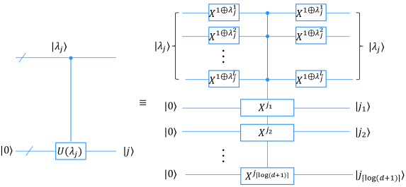
Figure 1: Quantum circuit for $CU_{j}$, where the upper register stores the eigenvalues $\left|\lambda_{j}\right\rangle$ and the lower one is the index register. Here / denotes a bundle of qubits, and $X$ denotes quantum NOT gate. $X^{1\oplus\lambda_{j}^{k}}=I(X)$ if $\lambda_{j}^{k}=1(0)$ for $k=1,2,\cdots,L$, and $X^{j_{l}}=I(X)$ if $j_{l}=0(1)$ for $l=1,2,\cdots,\lceil\log(d+1)\rceil$. The circuit implements the map $\left|0\right\rangle\mapsto\left|j\right\rangle\equiv\left|j_{1}j_{2}\cdots j_{\lceil\log(d+1)\rceil}\right\rangle$ on the index register if the eigenvalue register is in the state $\left|\lambda_{j}\right\rangle\equiv\left|\lambda_{j}^{1}\lambda_{j}^{2}\cdots\lambda_{j}^{L}\right\rangle$, and otherwise does nothing.

(3.3) Inverse phase estimation. We undo step (3.1), discard the eigenvalue register, and have the state

$$\frac{\sum_{i=1}^{N}y_{ij}\left|i\right\rangle\left|\mathbf{v}_{j}\right\rangle(\sum_{j=1}^{d}\left|j\right\rangle+\sum_{j=d+1}^{D}\left|0\right\rangle)}{\left\lVert X\right\rVert_{F}}.$$ (21)

(3.4) Controlled rotation. Append another qubit in the state $\left|0\right\rangle$ as the last register, and perform $d$ controlled unitary rotation operations $CR(\beta_{1}),CR(\beta_{2}),\cdots,CR(\beta_{d})$, conditioned on $\left|j\right\rangle$, where

$$CR(\beta_{j}):\left|j\right\rangle\left|0\right\rangle\mapsto\left|j\right\rangle\left(\frac{C}{\hat{\beta}_{j}}\left|1\right\rangle+\sqrt{1-\frac{C^{2}}{\hat{\beta}_{j}^{2}}}\left|0\right\rangle\right),$$ (22)

for $j=1,2,\cdots,d$. Here $\hat{\beta}_{j}$ denotes the estimate of $\beta_{j}$ obtained in step (2) and $C=O(\min_{j}\hat{\beta_{j}})=O(1/\sqrt{d})$. After rotation, we have the state of the whole system,

$$\sum_{i=1}^{N}\frac{y_{ij}}{\left\lVert X\right\rVert_{F}}\left|i\right\rangle\left|\mathbf{v}_{j}\right\rangle\left(\sum_{j=1}^{d}\left|j\right\rangle\Big{(}\frac{C}{\hat{\beta}_{j}}\left|1\right\rangle+\sqrt{1-\frac{C^{2}}{\hat{\beta}_{j}^{2}}}\left|0\right\rangle\Big{)}+\sum_{j=d+1}^{D}\left|0\right\rangle\left|0\right\rangle\right).$$ (23)

It should be noted that, since the classical information of each $\hat{\beta}_{j}$ is provided, each controlled rotation $CR(\beta_{j})$ can be directly constructed and efficiently implemented. This is much more resource-saving than the controlled rotations which are widely used in the HHL-based quantum algorithms HHL09 ; CD16 ; DYLL17 ; WBL12 ; SSP16 ; QRR17 ; Yuetal18 , but need quantum arithmetic circuits HRS18 taking substantially more qubits and runtime.

(3.5) Projective measurement. Measure the second register of $\left|\mathbf{v}_{j}\right\rangle$ to see whether it is in the state $\left|\mathbf{x}\right\rangle=U_{\mathbf{x}}\left|0\right\rangle$ by performing $U_{\mathbf{x}}^{-1}$ followed by the projective measurement $\left|0\right\rangle\left\langle 0\right|$. At the same time, measure the last qubit to see whether it is in the state $\left|1\right\rangle$ by performing the projective measurement $\left|1\right\rangle\left\langle 1\right|$. If both measurements succeed, we trace out these two registers and have the state of the other two registers

$$\frac{\sum\limits_{i=1}^{N}\sum\limits_{j=1}^{d}\frac{y_{ij}}{\left\lVert X\right\rVert_{F}}\frac{C\beta_{j}}{\hat{\beta}_{j}}\left|i\right\rangle\left|j\right\rangle}{\sqrt{\sum\limits_{i=1}^{N}\sum\limits_{j=1}^{d}\left(\frac{y_{ij}}{\left\lVert X\right\rVert_{F}}\frac{C\beta_{j}}{\hat{\beta}_{j}}\right)^{2}}} \approx \frac{\sum\limits_{i=1}^{N}\sum\limits_{j=1}^{d}y_{ij}\left|i\right\rangle\left|j\right\rangle}{\sqrt{\sum\limits_{i=1}^{N}\sum\limits_{j=1}^{d}y_{ij}^{2}}}.$$ (24)

The approximation holds because $\beta_{j}\approx\hat{\beta}_{j}$ as shown in step (2), and the right-hand side is exactly $\left|\psi_{e}\right\rangle$ by plugging Eq. (8) into the right-hand side of Eq. (6). This means that we finally obtain a state $\approx\left|\psi_{e}\right\rangle$ storing the new low-dimensional dataset $\{\mathbf{y}_{i}\}_{i=1}^{N}$ in quantum parallel, and thus complete the transformation of Eq. (6) we desire. Due to the linearity of the entire process, our algorithm can reduce the dimensionality of only a subset of the original data points,

$$\frac{\sum_{i\in S}\left|i\right\rangle\otimes\mathbf{x}_{i}}{\sqrt{\sum_{i\in S}\left\lVert\mathbf{x}_{i}\right\rVert^{2}}}\mapsto\frac{\sum_{i\in S}\left|i\right\rangle\otimes\mathbf{y}_{i}}{\sum_{i\in S}\sqrt{\left\lVert\mathbf{y}_{i}\right\rVert^{2}}},$$ (25)

where $S\subseteq\{1,2,\cdots,N\}$. Furthermore, for each individual data point prepared in the quantum state $\left|\mathbf{x}_{i}\right\rangle$, it is also straight forward to see that our algorithm implements

$$\left|\mathbf{x}_{i}\right\rangle\mapsto\left|\mathbf{y}_{i}\right\rangle,$$ (26)

without introducing the first register $\left|i\right\rangle$.

Now, we have finished describing the whole algorithm. The first two steps can be seen as supports to step (3), the key step in our algorithm. The quantum circuit for step (3) is shown in Fig. 2

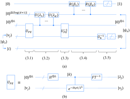
Figure 2: (a) Quantum circuit for step (3), where the unitary operation $U_{PE}$ represents the phase estimation algorithm and its quantum circuit is depicted in (b). The unitary operations controlled-$U(\lambda_{1}),\cdots,U(\lambda_{d})$ and controlled-$R(\beta_{1}),\cdots,R(\lambda_{d})$ correspond with $CU(\lambda_{1}),\cdots,CU(\lambda_{d})$ and $CR(\beta_{1}),\cdots,CR(\beta_{d})$, respectively. The five substeps of step (3) are marked as $(3.1),(3.2),\cdots,(3.5)$. (b) The quantum circuit for $U_{PE}$, where the unitary operations $H$ and $FT$ denotes the Hadamard gate and the quantum Fourier transformation QCQI10 , resepctively.

II.2 Runtime analysis

In step (1), according to QPCA14 , taking $O(1/\epsilon_{\lambda}^{3})$ copies of $\rho$ to implement the phase estimation algorithm QCQI10 ensures that the eigenvalues $\lambda_{j}$ can be estimated within error $\epsilon_{\lambda}$. Since preparing each copy of $\rho$ needs preparation of one copy of $\left|\psi_{s}\right\rangle$ with time complexity $O(\polylog(ND))$, generating the state of Eq. (15) takes runtime $O\left(\polylog(ND)/\epsilon_{\lambda}^{3}\right)$. In addition, as mentioned in step (1), sampling the state of Eq. (15) for $O(d)$ times guarantees that, with high probability, we can obtain each $\lambda_{j}$ and one copy of each $\left|\mathbf{v}_{j}\right\rangle$.

In step (2), based on the natural assumption that $\beta_{j}=O(1/\sqrt{d})$ for $j=1,2,\cdots,d$, each $\beta_{j}$ can be estimated within error $O(\epsilon_{\beta})$ with $O(1/\epsilon_{\beta}^{2})$ swap tests QSVM14 ; SSP16 ; BCWW01 , which takes $O(1/\epsilon_{\beta}^{2})$ copies of $\left|\mathbf{x}\right\rangle$ as well as $\left|\mathbf{v}_{j}\right\rangle$. Since generating one copy of $\left|\mathbf{x}\right\rangle$ takes $O(\polylog D)$ time and each swap test takes $O(\log D)$ elementary gates, the total runtime for step (2) is $O(d\polylog D/\epsilon_{\beta}^{2})$ under the condition that those copies of $\left|\mathbf{v}_{j}\right\rangle$ are provided by step (1). For step (1), the requirement of $O(1/\epsilon_{\beta}^{2})$ copies of $\left|\mathbf{v}_{j}\right\rangle$ implies the overall runtime

$$O\left(\frac{d\polylog(ND)}{\epsilon_{\beta}^{2}\epsilon_{\lambda}^{3}}\right).$$

The runtime for steps (3.1) and (3.3) obviously coincides with that for the procedure of generating the state of Eq. (15) in step (1). In step (3.2), each $CU_{j}$ for $j=1,2,\cdots,d$ takes $O(\log(1/\epsilon_{\lambda})\log(d+1))$ elementary gates QCQI10 ; QGate95 , so step (3.2) takes $O\left(d\log(1/\epsilon_{\lambda})\log(d+1)\right)$ time. According to QGate95 , step (3.4) generally takes $O(d\log(d+1))$ time. In step (3.5), just as $U_{\mathbf{x}}$ in step (2), the unitary operation $U_{\mathbf{x}}^{-1}$ also runs in time $O\left(\polylog D\right)$. Finally, the success probability of measurement in step (3.5) is

$$p: = \sum_{i=1}^{N}\sum_{j=1}^{d}\left(\frac{y_{ij}}{\left\lVert X\right\rVert_{F}}\frac{C\beta_{j}}{\hat{\beta}_{j}}\right)^{2}$$ (27)

$$\approx \frac{C^{2}\left\lVert Y\right\rVert_{F}^{2}}{\left\lVert X\right\rVert_{F}^{2}}$$

$$= O(1/d),$$

because $C=O(1/\sqrt{d})$, and

$$\frac{\left\lVert Y\right\rVert_{F}^{2}}{\left\lVert X\right\rVert_{F}^{2}}=\frac{\sum_{j=1}^{d}\sigma_{j}^{2}}{\sum_{j=1}^{D}\sigma_{j}^{2}}\geq\vartheta=O(1),$$

according to Eqs. (1) and (4). That is to say, $O(d)$ measurements are required to obtain $\left|\psi_{e}\right\rangle$ with high probability; the number of repetitions can be reduced to $O(\sqrt{d})$ via amplitude amplification AA02 .

Table 1: The time complexity of each step of our algorithm. Here the $\sqrt{d}$ factor occurring in each substep of step (3) corresponds to the number of repetitions for amplitude amplification in step (3.5).

Steps	Time complexity
(1)	$O(\epsilon_{\beta}^{-2}\epsilon_{\lambda}^{-3}d\polylog(ND))$
(2)	$O(d\polylog D/\epsilon_{\beta}^{2})$
(3.1)	$O(\sqrt{d}\cdot\polylog(ND)/\epsilon_{\lambda}^{3})$
(3.2)	$O(\sqrt{d}\cdot d\log(1/\epsilon_{\lambda})\log(d+1))$
(3.3)	$O(\sqrt{d}\cdot\polylog(ND)/\epsilon_{\lambda}^{3})$
(3.4)	$O(\sqrt{d}\cdot d\log(d+1))$
(3.5)	$O(\sqrt{d}\cdot\polylog D)$

Moreover, according to the analysis of the HHL algorithm HHL09 , the final error for generating $\left|\psi_{e}\right\rangle$ mainly comes from the inverse of $\beta_{j}$. Since $\beta_{j}$ is estimated with error $O(\epsilon_{\beta})$, the relative error of estimating $1/\beta_{j}$ is $O(\epsilon_{\beta}/\beta_{j})=O(\epsilon_{\beta}/\sqrt{d})$ and thus the final state $\left|\psi_{e}\right\rangle$ induces error $O(\epsilon_{\beta}/\sqrt{d})$. To ensure the final error be within $\epsilon$, we should take $\epsilon_{\beta}=O(\sqrt{d}\epsilon)$.

The time complexity of each step of our algorithm is shown in the Table 1. Putting all runtime together and taking $\epsilon_{\beta}=O(\sqrt{d}\epsilon)$ as shown above, our algorithm has the overall runtime

$$O\left(\epsilon^{-2}\epsilon_{\lambda}^{-3}\polylog(ND)+d^{3/2}\log(1/\epsilon_{\lambda})\log(d+1)\right).$$

In addition, if every $\lambda_{j}=O(1/d)$, $\epsilon_{\lambda}$ should take $O(1/d)$ and thus the overall runtime will be $O(d^{3}\polylog(ND)/\epsilon^{2})$. This means that it has runtime $O(\polylog(N,D))$ when $d=O(\polylog(D))$, achieving exponential speedup over the classical PCA algorithm whose runtime is $O(\poly(N,D))$ PRML06 ; HML17 .

According to the above analysis and the transformation of Eq. (26), it is easy to see that our algorithm can efficiently transform each quantum data point $\left|\mathbf{x}_{i}\right\rangle$ of the high-dimensional quantum dataset $\{\left|\mathbf{x}_{i}\right\rangle\}_{i=1}^{N}$ into a polylogarithmically lower-dimensional quantum data $\left|\mathbf{y}_{i}\right\rangle$ of polylogarithmically fewer qubits. This implies that, under certain conditions, our algorithm breaks the limits on quantum dimensionality reduction QDR15 . The result of QDR15 shows that the dimension of a set of high-dimensional quantum states cannot be significantly reduced while preserving the 2-norm distance of each pairwise states. This leaves an open question of whether significant dimension reduction is possible when multiple copies of the input states (whose dimensionality is to be reduced) are available QDR15 . Our algorithm gives an positive answer to this question, in the sense that, by taking take polylogarithmically fewer copies of the input states $\{\left|\mathbf{x}_{i}\right\rangle\}_{i=1}^{N}$, as shown above, our algorithm can map each state $\left|\mathbf{x}_{i}\right\rangle$ into the polylogarithmically lower-dimensional state $\left|\mathbf{y}_{i}\right\rangle$, while well preserving the 2-norm distances of most pairwise states. The 2-norm distances of most pairwise states are well preserved because our quantum algorithm is based on PCA which guarantees that $\left\langle\mathbf{y}_{i_{1}}|\mathbf{y}_{i_{2}}\right\rangle\approx\left\langle\mathbf{x}_{i_{1}}|\mathbf{x}_{i_{2}}\right\rangle$ for most $i_{1},i_{2}\in\{1,2,\cdots,n\}$. Note that $\left\lVert\left|a\right\rangle-\left|b\right\rangle\right\rVert_{2}=\sqrt{2(1-\left\langle a|b\right\rangle)}$ for any two same-dimensional quantum states with real amplitudes.

III Adaptation to quantum machine learning

In this section, we show that, to reduce the data dimensionality, our quantum algorithm can be applied to two well-known supervised quantum machine learning algorithms, quantum support vector machine (QSVM) QSVM14 and quantum linear regression for prediction SSP16 .

III.1 Quantum support vector machine

Support vector machine (SVM) is an important supervised machine learning algorithm for data classification. Given $N$ training data points $\{(\mathbf{x}_{i},z_{i}):\mathbf{x}_{i}\in\mathbb{R}^{D},z_{i}=\pm 1\}_{i=1}^{N}$, where $z_{i}$ identifies which class $\mathbf{x}_{i}$ belongs to, the task of SVM is to classify a vector into one of two classes. The least-squares approximation of SVM is found by solving the following system of linear equations:

$$F\left(\begin{matrix}a\\ \mathbf{b}\end{matrix}\right)=\left(\begin{matrix}0&\mathbf{1}\\ \mathbf{1}&K+\gamma I\end{matrix}\right)\left(\begin{matrix}a\\ \mathbf{b}\end{matrix}\right)=\left(\begin{matrix}0\\ \mathbf{z}\end{matrix}\right).$$ (28)

Here, $\mathbf{1}=(1,\cdots,1)^{T}$, $\gamma\in\mathbb{R}$ is a constant, $K_{ij}=\mathbf{x}_{i}^{T}\mathbf{x}_{j}$; $a\in\mathbb{R}$ and $\mathbf{b}=(b_{1},\cdots,b_{N})$; and $\mathbf{z}=(z_{1},\cdots,z_{N})$. When obtaining $a$ and $\mathbf{b}$, one can predict the class of a new data point $\mathbf{x}_{0}$ by $z_{0}=\text{sgn}(\sum_{j=1}^{N}b_{j}\mathbf{x}_{0}^{T}\mathbf{x}_{j}+a)$.

Following the above approach, the QSVM algorithm QSVM14 can be briefly summarized by the following steps and the corresponding schematic quantum circuit is shown in Fig. 3.

(1) Assuming quantum oracles accessing the training data points, denoted by $O_{\textbf{x}}$, are provided, QSVM generates a number of copies of the quantum state $\left|\chi_{1}\right\rangle=\sum_{i=1}^{N}\left|i\right\rangle\otimes\mathbf{x}_{i}/\sqrt{\sum_{i=1}^{N}\left\lVert\mathbf{x}_{i}\right\rVert^{2}}$.

(2) By using the quantum matrix insertion approach HHL09 together with exponentiation of the density matrix $K/\textmd{Tr}(K)=\textmd{Tr}_{2}(\left|\chi_{1}\right\rangle\left\langle\chi_{1}\right|)$ QPCA14 , QSVM solves the above linear system of equations (i.e., Eq. (28)), creates the quantum state $\left|a,\mathbf{b}\right\rangle=a\left|0\right\rangle+\sum_{j=1}^{N}b_{j}\left|j\right\rangle$, and, by calling $O_{\textbf{x}}$, further generates

$$\left|\psi_{1}\right\rangle=\frac{a\left|0\right\rangle\otimes\left|0\right\rangle+\sum_{j=1}^{N}b_{j}\left|j\right\rangle\otimes\mathbf{x}_{j}}{\sqrt{a^{2}+\sum_{j=1}^{N}b_{j}^{2}\left\lVert\mathbf{x}_{j}\right\rVert^{2}}}.$$

(3) Prepare the state $\left|\psi_{2}\right\rangle=(\left|0\right\rangle\otimes\left|0\right\rangle+\sum_{j=1}^{N}\left|j\right\rangle\otimes\mathbf{x_{0}})/\sqrt{1+N\left\lVert\mathbf{x_{0}}\right\rVert^{2}}$, and obtain $\left\langle\psi_{1}\right|\psi_{2}\rangle$ via swap test QSVM14 , which reveals $z_{0}$, the predictive class of the data point $\mathbf{x}_{0}$.

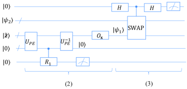
Figure 3: Schematic quantum circuit for QSVM, where $U_{PE}$ represents the phase estimation algorithm whose circuit is same as Fig. 2 (b) except that the unitary operation controlled is now $e^{-iF/\textmd{Tr}(F)t}$ for some $t$. Here the state $\left|\tilde{\mathbf{z}}\right\rangle$ corresponds to the normalized right-hand side of Eq. (28), controlled-$R_{1}$ denotes the controlled rotation required in step (2) for matrix inversion QSVM14 , and SWAP corresponds to the swap operation. The numbers (2) and (3) respectively mark steps (2) and (3).

Our quantum algorithm can be applied to QSVM to reduce the data dimensionality. Specifically, in step (1) our algorithm transforms $\left|\chi_{1}\right\rangle$ into another state $\left|\chi_{1}^{\prime}\right\rangle=\sum_{i=1}^{N}\left|i\right\rangle\otimes\mathbf{y}_{i}/\left\lVert Y\right\rVert_{F}$, where $\mathbf{y}_{i}$ is the low-dimensional data representation of $\mathbf{x}_{i}$ by PCA. In addition, step (2) will instead proceed with exponentiation of the density matrix $\textmd{Tr}_{2}(\left|\chi_{1}^{\prime}\right\rangle\left\langle\chi_{1}^{\prime}\right|)$, which encodes the low-dimensional data points $\{\mathbf{y}_{1},\cdots,\mathbf{y}_{N}\}$, and $\mathbf{x}_{j}$ in the state $\left|\psi_{1}\right\rangle$ will be replaced with $\mathbf{y}_{j}$. Finally, in step 3, $\mathbf{x}_{0}$ is projected to the low-dimensional space with the data point $\mathbf{y}_{0}$ in the state $\left|\psi_{2}\right\rangle$, and $\mathbf{y}_{0}$ can be successfully classified via swap tests.

III.2 Quantum linear regression algorithm for prediction

Linear regression is another important supervised learning task. Given $N$ training data points, for simplicity also denoted by $\{(\mathbf{x}_{i},z_{i}):\mathbf{x}_{i}\in\mathbb{R}^{D},z_{i}\in\mathbb{R}\}_{i=1}^{N}$, the objective is to construct a linear model $f(x)=\mathbf{x}^{T}\mathbf{w}$ that can best describe the linear relationship between $\mathbf{x}_{i}$ and $z_{i}$ and use this model to predict $z_{0}=f(\mathbf{x}_{0})$ for a new input $\mathbf{x}_{0}$. Using the least-squares method, the optimal $\mathbf{w}$ is given by $\mathbf{w}=(X^{T}X)^{-1}X^{T}\mathbf{z}$, where $X=(\mathbf{x}_{1},\cdots,\mathbf{x}_{N})^{T}$ and $\mathbf{z}=(z_{1},\cdots,z_{N})$, and thus $z_{0}=\sum_{j=1}^{D}\mathbf{w}^{T}\mathbf{x}_{0}$. Taking the singular value decomposition form, $X=\sum_{j=1}^{R}\sigma_{j}\left|\mathbf{u}_{j}\right\rangle\left\langle\mathbf{v}_{j}\right|$, where $R$ is the rank of $X$, $z_{0}=\sigma_{j}^{-1}\mathbf{x}_{0}^{T}\left|\mathbf{v}_{j}\right\rangle\left\langle\mathbf{u}_{j}\right|\mathbf{z}$.

In the context of quantum computing, Schuld et al. in 2016 proposed a quantum algorithm (QLR) SSP16 for implementing the above task, where, for simplicity, $\left\lVert X\right\rVert_{F}$, $\left\lVert\mathbf{z}\right\rVert$ and $\left\lVert\mathbf{x}_{0}\right\rVert$ are all assumed to be 1. The algorithm can be outlined as follows and the corresponding schematic quantum circuit is depicted in Fig. 4.

(1) Assuming quantum oracles accessing the training data points, also denoted by $O_{\textbf{x}}$, are provided, QLR generates the initial quantum state $\left|\chi_{2}\right\rangle=\sum_{i=1}^{N}\mathbf{x}_{i}\otimes\left|i\right\rangle/\sqrt{N}=\sum_{j=1}^{R}\sigma_{j}\left|\mathbf{v}_{j}\right\rangle\left|\mathbf{u}_{j}\right\rangle$.

(2)Using the quantum matrix insertion approach HHL09 together with the exponentiation of the density matrix $\textmd{Tr}_{2}(\left|\chi_{2}\right\rangle\left\langle\chi_{2}\right|)$ SSP16 , QLR transforms $\left|\chi_{2}\right\rangle$ into another state $\left|\phi_{1}\right\rangle\propto\sum_{j=1}^{R}1/\sigma_{j}\left|\mathbf{v}_{j}\right\rangle\left|\mathbf{u}_{j}\right\rangle$.

(3) Prepare the state $\left|\phi_{2}\right\rangle=\left|\mathbf{x}_{0}\right\rangle\left|\mathbf{z}\right\rangle$ with $\left|\mathbf{z}\right\rangle$ being the quantum-state form of (normalized) $\mathbf{z}$, and then estimate $\left\langle\phi_{1}\right|\phi_{2}\rangle\propto z_{0}$ up to some measurable factor SSP16 , via swap test QSVM14 with an ancilla qubit.

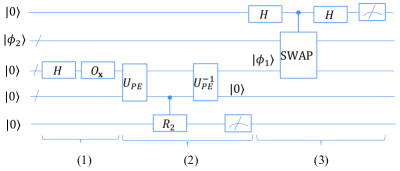
Figure 4: Schematic quantum circuit for QLR, where $U_{PE}$ also represents the phase estimation algorithm (as shown in Fig. 2 (b)) for the unitary operation $e^{-i\textmd{Tr}_{2}(\left|\chi_{2}\right\rangle\left\langle\chi_{2}\right|)t}$ for some $t$. Also, the controlled-$R_{2}$ also denotes the controlled rotation involved in matrix inversion SSP16 ; HHL09 in step (2), and the numbers (1)-(3) correspond to the three steps.

Our quantum algorithm can also be applied to QLR. In step (1), by our quantum algorithm, the state $\left|\chi_{2}\right\rangle$ is transformed into $\left|\chi_{2}^{\prime}\right\rangle\propto\sum_{i=1}^{N}\mathbf{y}_{i}\otimes\left|i\right\rangle$, where $\mathbf{y}_{i}$ is the low-dimensional data corresponding to $\mathbf{x}_{i}$. Step (2) will work with the density matrix $Tr_{2}(\left|\chi_{2}^{\prime}\right\rangle\left\langle\chi_{2}^{\prime}\right|)$, which encodes the low-dimensional data points $\{\mathbf{y}_{1},\cdots,\mathbf{y}_{N}\}$, and transform $\left|\chi_{2}^{\prime}\right\rangle$ into $\left|\phi_{1}^{\prime}\right\rangle$. In the last step, we by our algorithm generate the state $\left|\phi_{2}^{\prime}\right\rangle:=\left|\mathbf{y}_{0}\right\rangle\left|\mathbf{z}\right\rangle$ from $\left|\phi_{2}\right\rangle$, where $\left|\mathbf{y}_{0}\right\rangle$ is the normalized quantum state representation of low-dimensional $\mathbf{x}_{0}$. Just as predicting $\mathbf{x}_{0}$, $\left|\phi_{2}^{\prime}\right\rangle$ is then taken into swap tests with $\left|\phi_{1}^{\prime}\right\rangle$ to predict the target of $\left|\mathbf{y}_{0}\right\rangle$.

In addition to the above two examples, it is promising that, to reduce the data dimensionality and avoid the curse of dimensionality, our algorithm could also be applied to other QML algorithms, where the states as $\left|\psi_{s}\right\rangle$, storing the data points in quantum parallel, are involved.

IV Conclusions

We have presented a quantum algorithm that compresses a large high-dimensional dataset in quantum parallel by reducing their dimensionality based on PCA. The algorithm is shown to be exponentially faster than the classical PCA algorithm, when the compressed dataset is of polylogarithmically low dimensionality. The compressed dataset can then be further processed to implement other tasks of interest with significantly less quantum resource. As examples, we show that the algorithm can be applied to reduce the data dimensionality of two well-known quantum machine learning algorithms, quantum support vector machine and quantum linear regression for prediction. This demonstrates that our algorithm has the potential to be well adapted to QML, and to free it from the curse of dimensionality to solve some problems of practical importance. Since PCA underlies a variety of linear or nonlinear DR algorithms, our quantum algorithm may be promising to inspire more quantum data compression algorithms based on other linear or nonlinear DR approaches.

References

- (1) Y. C. Ma and M. H. Yung, Transforming Bell’s inequalities into state classifiers with machine learning, npj Quantum Information 4, 34 (2018).
- (2) S. Lu et al., Separability-entanglement classifier via machine learning, Phys. Rev. A 98, 012315 (2018).
- (3) N. Wiebe, C. Granade, C. Ferrie, and D. G. Cory, Quantum Hamiltonian learning using imperfect quantum resources, Phys. Rev. A 89, 042314 (2014).
- (4) N. Wiebe, C. Granade, C. Ferrie, and D. G. Cory, Hamiltonian learning and certification using quantum resources, Phys. Rev. Lett. 112, 190501 (2014).
- (5) J. Wang et al., Experimental quantum Hamiltonian learning, Nature Physics 13 551 (2017).
- (6) A. Bisio et al., Optimal quantum learning of a unitary transformation, Phys. Rev. A 81, 032324 (2010).
- (7) J. Bang et al., A strategy for quantum algorithm design assisted by machine learning, New J. Phys. 16, 073017 (2014).
- (8) A. W. Harrow, A. Hassidim, and S. Lloyd, Quantum algorithm for linear systems of equations, Phys. Rev. Lett. 103, 150502 (2009).
- (9) S. Lloyd, M. Mohseni, and P. Rebentrost, Quantum algorithms for supervised and unsupervised machine learning, arXiv:1307.0411 (2013).
- (10) P. Rebentrost, M. Mohseni, and S. Lloyd, Quantum support vector machine for big data classification, Phys. Rev. Lett. 113, 130503 (2014).
- (11) I. Cong and L. Duan, Quantum discriminant analysis for dimensionality reduction and classification, New J. Phys. 18, 073011 (2016).
- (12) M. Schuld, M. Fingerhuth, F. Petruccione, Implementing a distance-based classifier with a quantum interference circuit, Europhys. Lett. 119, 60002 (2017).
- (13) B. Duan, J. Yuan, Y. Liu, and D. Li, Quantum algorithm for support matrix machines, Phys. Rev. A 96, 032301 (2017).
- (14) M. Schuld, A. Bocharov, K. Svore, and N. Wiebe,Circuit-centric quantum classifiers, arXiv:1804.00633, (2018).
- (15) M. Schuld and F. Petruccione, Quantum ensembles of quantum classifiers, Sc. Rep. 8, 2772 (2018).
- (16) N. Wiebe, D. Braun, and S. Lloyd, Quantum algorithm for data fitting, Phys. Rev. Lett. 109, 050505 (2012).
- (17) M. Schuld, I. Sinayskiy, and F. Petruccione, Prediction by linear regression on a quantum computer, Phys. Rev. A 94, 022342 (2016).
- (18) G. Wang, Quantum algorithm for linear regression, Phys. Rev. A 96, 012335 (2017).
- (19) C.-H. Yu, F. Gao, and Q.-Y. Wen. Quantum algorithm for ridge regression, arXiv:1707.09524 (2017).
- (20) C.-H. Yu et al., Quantum algorithm for visual tracking, arXiv:1807.00476 (2018).
- (21) E Aïmeur E, G. Brassard and S. Gambs, Quantum speed-up for unsupervised learning, Mach. Learn. 90, 261 (2013).
- (22) C.-H. Yu, F. Gao, Q.-L. Wang and Q.-Y. Wen, Quantum algorithm for association rules mining, Phys. Rev. A 94, 042311 (2016).
- (23) N. Liu and P. Rebentrost, Quantum machine learning for quantum anomaly detection, Phys. Rev. A 97, 042315.
- (24) X.-D. Cai et al., Entanglement-Based Machine Learning on a Quantum Computer, Phys. Rev. Lett. 114, 110504 (2015).
- (25) Z. Li, et al., Experimental realization of a quantum support vector machine, Phys. Rev. Lett. 114, 140504 (2015).
- (26) V. Dunjko and H. J Briegel, Machine learning & artificial intelligence in the quantum domain: a review of recent progress, Rep. Prog. Phys. 81, 074001 (2018).
- (27) J. Biamonte, P. Wittek, N. Pancotti, P. Rebentrost, N. Wiebe, and Seth Lloyd, Quantum machine learning, Nature 549, 195-202 (2017).
- (28) C. M. Bishop, Pattern Recognition and Machine Learning (Springer, 2006).
- (29) A. Gron, Hands-on machine learning with Scikit-Learn and TensorFlow: concepts, tools, and techniques to build intelligent systems (O’Reilly Media, Inc., 2017).
- (30) S. Lloyd, M. Mohseni, and P. Rebentrost, Quantum principal component analysis, Nature Physics 10, 631 (2014).
- (31) A. Daskin, Obtaining a linear combination of the principal components of a matrix on quantum computers, Quantum Inform. Process. 15, 4013 (2016).
- (32) G. Brassard, P. Høyer, M. Mosca, and A. Tapp, Quantum Amplitude Aplification and Estimation, Contemporary Mathematics Series Millenium Volumn 305 (AMS, New York, 2002).
- (33) H. Buhrman, R. Cleve, J. Watrous, and R. de Wolf, Quantum fingerprinting, Phys. Rev. Lett. 87, 167902 (2001).
- (34) Lee A. Rozema, et. al., Quantum Data Compression of a Qubit Ensemble, Phys. Rev. Lett. 113, 160504 (2014).
- (35) Y. Yang, G. Chiribella, M. Hayashi, Optimal compression for identically prepared qubit states, Phys. Rev. Lett. 117, 090502 (2016).
- (36) Y. Yang, G. Chiribella, D. Ebler, Efficient quantum compression for ensembles of identically prepared mixed states, Phys. Rev. Lett. 116, 080501 (2016).
- (37) V. Giovannetti, S. Lloyd and L. Maccone, Quantum random access memory, Phys. Rev. Lett. 100, 160501 (2008).
- (38) I. Kerenidis and A. Prakash, Quantum recommendation systems, arXiv:1603.08675 (2016).
- (39) L. Wossnig, Z. Zhao and A. Prakash, Quantum linear system algorithm for dense matrices, Phys. Rev. Lett. 120, 050502 (2018).
- (40) T. Häner , M. Roetteler, and K. M. Svore. Optimizing quantum circuits for arithmetic arXiv:1805.12445, (2018).
- (41) M. A. Nielsen and I. L Chuang, Quantum computation and quantum information (Cambridge university press, 2010).
- (42) A. Barenco, C. H. Bennett, R. Cleve, D. P. DiVincenzo, N. Margolus, P Shor, T. Sleator, J. A. Smolin, and H. Weinfurter, Elementary gates for quantum compution, Phys. Rev. A 52, 3457 (1995).
- (43) A. W. Harrow, A. Montanaro and A. J. Short, Limitations on quantum dimensionality reduction, Int. J. of Quantum Inform. 13, 1440001 (2015).