A New Class of Symmetric Distributions Including the Elliptically Symmetric Logistic

Abstract

We introduce a new broad and flexible class of multivariate elliptically symmetric distributions including the elliptically symmetric logistic and multivariate normal. Various probabilistic properties of the new distribution are studied, including the distribution of linear transformations, marginal distributions, conditional distributions, moments, stochastic representations and characteristic function.

Keywords: elliptically symmetric logistic distributions; elliptically symmetric distributions; logistic distribution; spherically symmetric distribution

1 Introduction

The elliptically symmetric logistic distribution with density

$$f({\bf x})=\frac{\Gamma(\frac{n}{2})|\Sigma|^{-\frac{1}{2}}}{\pi^{\frac{n}{2}}\int_{0}^{\infty}u^{\frac{n}{2}-1}\frac{\exp(-u)}{(1+\exp(-u))^{2}}du}\frac{\exp(-({\bf x}-{\boldsymbol{\mu}})^{T}{\bf\Sigma}^{-1}({\bf x-{\boldsymbol{\mu}}}))}{(1+\exp(-({\bf x}-{\boldsymbol{\mu}})^{T}{\bf\Sigma}^{-1}({\bf x-{\boldsymbol{\mu}}})))^{2}},\;{\bf x}\in\mathbb{R}^{n},$$

has been originally introduced by Jensen (1985) (as the generalization of the multivariate normal distribution) and studied by Fang et al. (1990), Arnold (1992), Kano (1994), Volodin (1999) and Gómez-Sánchez-Manzano et al. (2006). Several applications of multivariate symmetric logistic distribution in risk management, quantitative finance and actuarial science can be found in many literatures such as Valdez and Chernih(2003), Landsman (2004), Landsman and Valdez (2003) and Landsman et al. (2003, 2016, 2018), Xiao and Valdez (2015). Note that several authors (cf. Gumbel (1961) Malik and Abraham (1973), Ali et al. (1978), Fang and Xu (1989), Kotz, Balakrishnan and Johnson (2000), Yeh (2010), Hu and Lin (2018), Ghosh and Alzaatreh (2018)) have studied the multivariate logistic distribution using different definitions.

The elliptically symmetric logistic distribution belongs to the elliptically contoured distributions family (also called an elliptically symmetric distributions family) $Ell_{n}({\boldsymbol{\mu}},{\bf\Sigma},g)$ with the location parameter ${\boldsymbol{\mu}}$, the scale parameter ${\bf\Sigma}$ and the density generator

$$g(u)=\frac{\exp(-u)}{(1+\exp(-u))^{2}}.$$

However, research work on the multivariate symmetric logistic distribution in recent decade is rather scarce compared to much research has focused on other elliptical distributions such as multivariate normal, multivariate Student $t$, multivariate Cauchy, multivariate power exponential distribution, Kotz-type distribution and multivariate skew-normal distributions; see the books and papers of Fang, Kotz and Ng (1990), Johnson, Kotz and Balakrishnan (1995) and Kotz, Balakrishnan and Johnson (2000), Azzalini and Regoli (2002), Arellano-Valle and Azzalini (2013), Battey and Linton (2014), Arashi and Nadarajah (2016), Arellano-Valle et al.(2018) and the references therein. The relative few literatures on the properties of elliptically symmetric logistic distribution drive the authors to further study the properties of this distribution. Moreover, we will define a new family of multivariate distributions including the elliptically symmetric logistic and multivariate normal and study the probabilistic properties of the distributions included by this family.

In some literature, the joint pdf of $n$-dimensional elliptically symmetric logistic distribution is defined as

$$f({\bf x})=c_{n}|\Sigma|^{-\frac{1}{2}}\frac{\exp(-\frac{1}{2}q({\bf x}))}{(1+\exp(-\frac{1}{2}q({\bf x})))^{2}},{\bf x}\in\mathbb{R}^{n},$$

where $q({\bf x})=({\bf x}-{\boldsymbol{\mu}})^{T}{\bf\Sigma}^{-1}({\bf x-{\boldsymbol{\mu}}})$. The density generator is

$$g_{n}(u)=\frac{\exp(-u)}{(1+\exp(-u))^{2}},$$

and the normalizing constant $c_{n}$ is given by

$$c_{n}=\frac{\Gamma(\frac{n}{2})}{(2\pi)^{\frac{n}{2}}}\left[\int_{0}^{\infty}x^{\frac{n}{2}-1}g_{n}(x)dx\right]^{-1}.$$ (1.1)

Interested readers may refer to Landsman and Valdez (2003) and Landsman et al. (2003, 2016, 2018), for more details on the elliptically symmetric logistic distribution and its applications. As pointed out by Landsman and Valdez (2003) this normalizing constant has been mistakenly pointed in Fang et al. (1990), Gupta et al. (2013), Xiao and Valdez (2015). Further simplification of the normalizing constant $c_{n}$ suggests by Landsman and Valdez (2003):

$$c_{n}=(2\pi)^{-\frac{n}{2}}\left[\sum_{j=1}^{\infty}(-1)^{j-1}j^{1-\frac{n}{2}}\right]^{-1}$$ (1.2)

by using the expansion

$$\frac{e^{-x}}{(1+e^{-x})^{2}}=\sum_{j=1}^{\infty}(-1)^{j-1}je^{-jx},\;x>0.$$ (1.3)

We observe that the formula (1.2) has no meaning when $n=1$ and 2, since the series

$$\sum_{j=1}^{\infty}(-1)^{j-1}\sqrt{j}\;\;{\rm and}\;\;\sum_{j=1}^{\infty}(-1)^{j-1}$$

are divergent.

We now give the definition of a generalized elliptically symmetric logistic distribution including the elliptically symmetric logistic distribution and multivariate normal.

Definition 1.1 The $n$-dimensional random vector $\bf{X}$ is said to have a generalized elliptically symmetric logistic distribution with location parameter $\boldsymbol{\mu}$ ($n$-dimensional vector) and dispersion matrix $\bf{\Sigma}$ ($n\times n$ matrix with $\bf{\Sigma}>0$) if its pdf has the form

$$f({\bf x})=d_{n}|{\bf\Sigma}|^{-\frac{1}{2}}g(({\bf x}-{\boldsymbol{\mu}})^{T}{\bf\Sigma}^{-1}({\bf x-{\boldsymbol{\mu}}})),\;{\bf x}\in\mathbb{R}^{n},$$ (1.4)

where $d_{n}$ is the normalizing constant and will be determined in the next section, $a,b,r>0$ are constants and

$$g(u)=\frac{\exp(-bu)}{(1+\exp(-au))^{r}},$$ (1.5)

is its density generator. If $\bf X$ belongs to the generalized elliptically symmetric logistic distribution, we shall write ${\bf{X}}\sim GML_{n}({\boldsymbol{\mu}},{\bf\Sigma},g)$.

The generalized elliptically symmetric logistic distribution is a particular case of an elliptically distribution, so $\bf X$ admits the stochastic representation

$${\bf X}={\boldsymbol{\mu}}+\sqrt{R}{\bf A}^{\prime}{\bf U}^{(n)},$$ (1.6)

where ${\bf A}$ is a square matrix such that ${\bf A}^{\prime}{\bf A}={\bf\Sigma}$, ${\bf U}^{(n)}$ is uniformly distributed on the unit sphere surface in $\mathbb{R}^{n}$, and $R\geq 0$ is independent of ${\bf U}^{(n)}$ and has the pdf given by

$$f_{R}(v)=\frac{1}{\int_{0}^{\infty}t^{\frac{n}{2}-1}g(t)dt}v^{\frac{n}{2}-1}g(v),v\geq 0.$$ (1.7)

For more details see Cambanis et al. (1981). Note that the $n$-dimensional elliptically symmetric logistic distribution can be deduced as a special case of (1.4) by setting $a=b=1$ and $r=2$; For $b=\frac{1}{2}$ and $r=0$, we obtain the multivariate normal distribution; The density generator (1.5) covers all the density generators of the generalized logistic types I-IV distributions in Arashi and Nadarajah (2017). Figures 1-5 illustrate the density functions of (1.4) with $n=2,a=b=1$ and $r=0.5,1,2,5,10$.

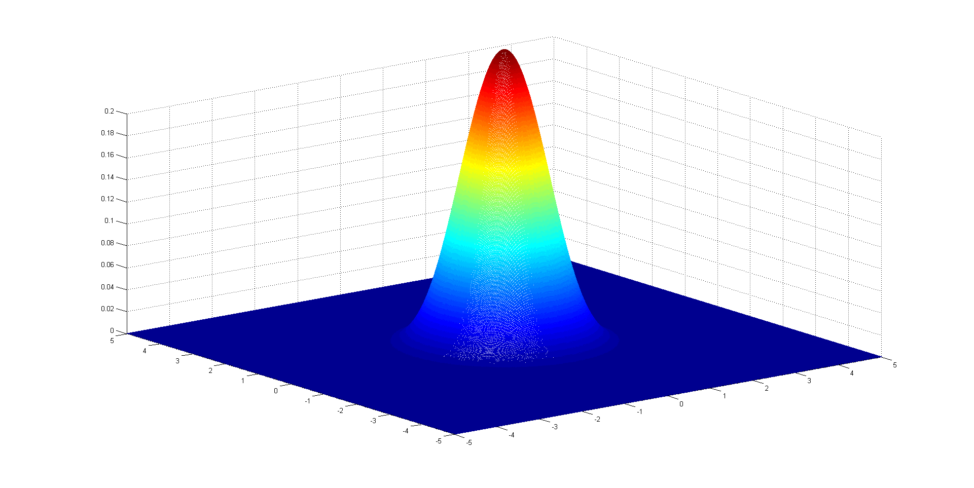
Figure 1: $r=0.5$

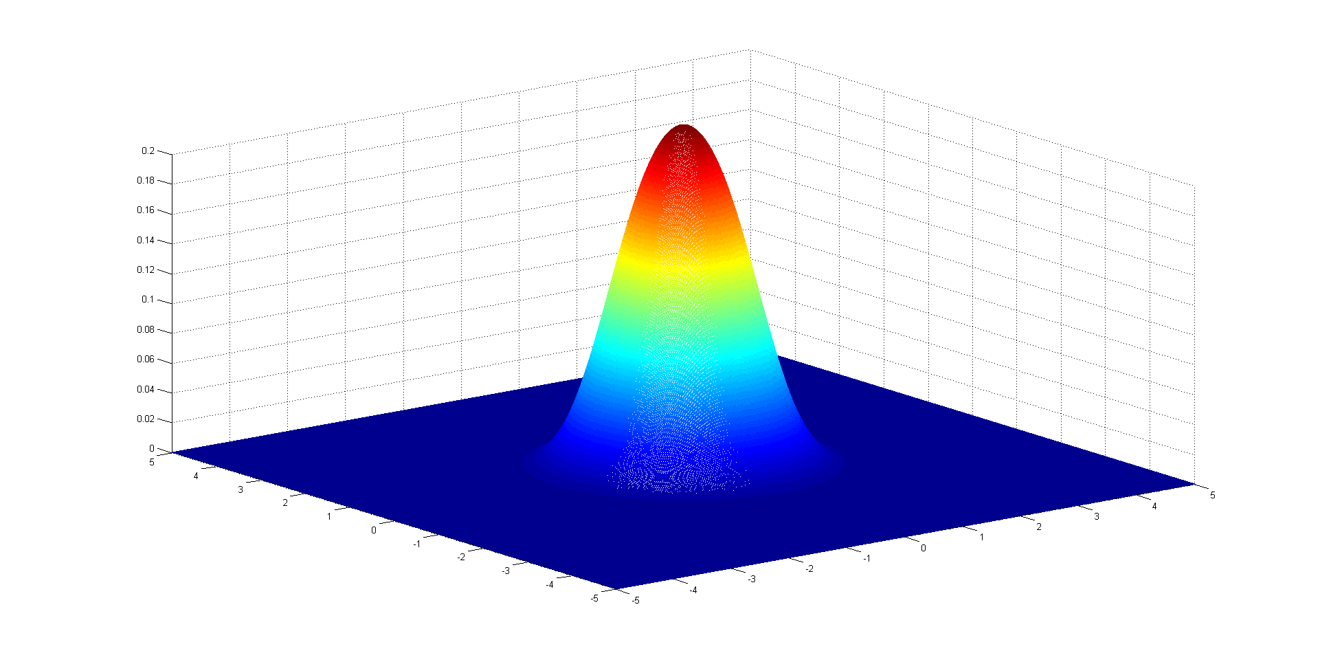
Figure 2: $r=1$

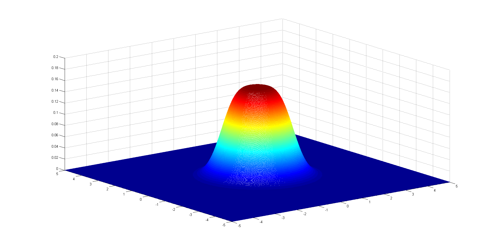
Figure 3: $r=2$

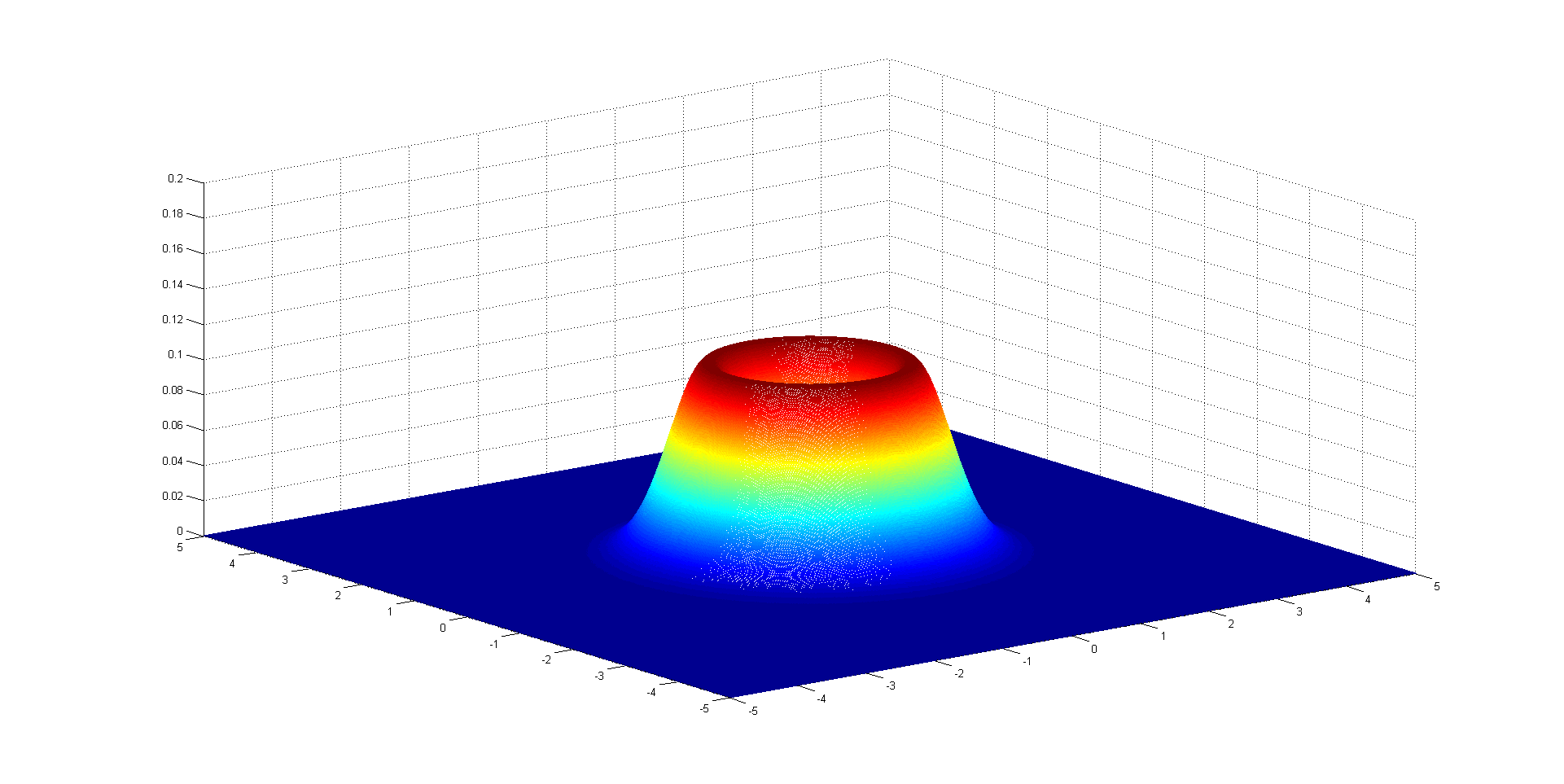
Figure 4: $r=5$

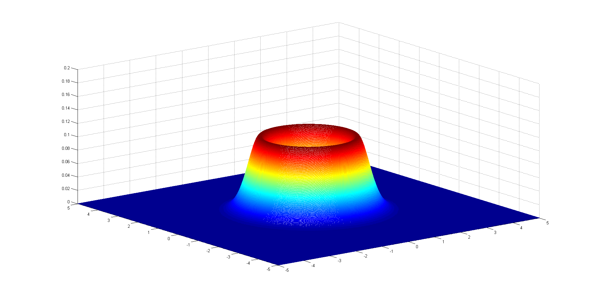
Figure 5: $r=10$

The rest of the paper is organized as follows. In Section 2, we discuss the expression of the normalizing constant in (1.1) and give the correct values for $c_{1}$ and $c_{2}$, and provide a equivalent expression for $c_{n},n\geq 3.$ In Sections 3-6 we will investigate some of the properties of this new class of the multivariate distributions. More specifically, we find the distributions of linear transformations, the marginal and conditional distributions, the moments and the characteristic functions.

2 Evaluation of the normalizing constants

We first collect some facts of the Riemann zeta function and the generalized Hurwitz-Lerch Zeta function which will be used in the sequel. The Riemann Zeta function $\zeta$ is defined as

$$\zeta(s)=\left\{\begin{array}[]{ll}\sum_{n=1}^{\infty}\frac{1}{n^{s}}=\frac{1}{1-2^{-s}}\sum_{n=1}^{\infty}\frac{1}{(2n-1)^{s}},&{\rm if}\;{\cal{R}}(s)>1,\\ \frac{1}{1-2^{1-s}}\sum_{n=1}^{\infty}\frac{(-1)^{n+1}}{n^{s}},&{\rm if}\;{\cal{R}}(s)>0,s\neq 1,\end{array}\right.$$

which can, except for a simple pole at $s=1$ with its residue 1, be continued meromorphically to the whole complex $s$-plane; see, for details Srivastava(2003), Choi et al. (2004). Recall that (see Arakawa et al. (2014), Cvijović and Klinowski (2002))

$$\zeta(2n)=(-1)^{n+1}\frac{2^{2n-1}}{(2n)!}\pi^{2n}B_{2n},n\in\mathbb{N}_{0},$$ (2.2)

and

$$\zeta(2n+1)=(-1)^{n+1}\frac{(2\pi)^{2n+1}}{2(2n+1)!}\int_{0}^{1}B_{2n+1}(u)\cot(\pi u)du,n\in\mathbb{N},$$ (2.3)

where $B_{n}=B_{n}(0)$ are the $n$th Bernoulli numbers and $B_{n}(x)$ are Bernoulli polynomials defined by the generating function

$$\frac{te^{tx}}{e^{t}-1}=\sum_{n=0}^{\infty}B_{n}(x)\frac{t^{n}}{n!},\;|t|<2\pi.$$

The Bernoulli numbers are well-tabulated (see, for example, Srivastava(2003)):

$$B_{0}=1,B_{1}=-\frac{1}{2},B_{2}=\frac{1}{6},B_{4}=-\frac{1}{30},B_{6}=\frac{1}{42},B_{2n+1}=0\;(n=1,2,\cdots),\cdots.$$

The functions $\zeta(s)$ has the following integral representations (cf. Srivastava and Choi (2012, p.169, p.172))

$$\zeta(s)=\frac{1}{\Gamma(s)}\int_{0}^{\infty}\frac{t^{s-1}}{e^{t}-1}dt,\;\;{\cal{R}}(s)>1,$$

and

$$\zeta(s)=\frac{(1-2^{1-s})^{-1}}{\Gamma(s+1)}\int_{0}^{\infty}\frac{t^{s}e^{t}}{(e^{t}+1)^{2}}dt,\;\;{\cal{R}}(s)>0.$$

Note that there is an extra 2 in (51) of Srivastava and Choi (2012, p.172).

The generalized Hurwitz-Lerch Zeta function is defined by (cf. Lin et al.(2006))

$$\Phi^{*}_{\mu}(z,s,a)=\frac{1}{\Gamma(\mu)}\sum_{n=0}^{\infty}\frac{\Gamma(\mu+n)}{n!}\frac{z^{n}}{(n+a)^{s}},$$

which has an integral representation

$$\Phi^{*}_{\mu}(z,s,a)=\frac{1}{\Gamma(s)}\int_{0}^{\infty}\frac{t^{s-1}e^{-at}}{(1-ze^{-t})^{\mu}}dt,$$ (2.4)

where ${\cal{R}}(a)>0$; ${\cal{R}}(s)>0$ when $|z|\leq 1(z\neq 1);{\cal{R}}(s)>1$ when $z=1).$

Theorem 2.1.

Consider the normalizing constant $d_{n}$ defined in (1.4).
Then

$$d_{n}=\left(\frac{a}{\pi}\right)^{\frac{n}{2}}\left[\Phi^{*}_{r}\left(-1,\frac{n}{2},\frac{b}{a}\right)\right]^{-1},$$ (2.5)

where $\Phi^{*}_{r}$ is the generalized Hurwitz-Lerch Zeta function.

Proof  By using the formula (1.37) in Denuit et al. (2005), we have

$$d_{n} = \frac{\Gamma(\frac{n}{2})}{(\pi)^{\frac{n}{2}}}\left[\int_{0}^{\infty}x^{\frac{n}{2}-1}g(x)dx\right]^{-1}$$

$$= \frac{\Gamma(\frac{n}{2})}{(\pi)^{\frac{n}{2}}}\left[\int_{0}^{\infty}x^{\frac{n}{2}-1}\frac{\exp(-bx)}{(1+\exp(-ax))^{r}}dx\right]^{-1}$$

$$= \frac{\Gamma(\frac{n}{2})a^{\frac{n}{2}}}{\pi^{\frac{n}{2}}}\left[\int_{0}^{\infty}x^{\frac{n}{2}-1}\frac{\exp(-\frac{b}{a}x)}{(1+\exp(-x))^{r}}dx\right]^{-1}$$

$$= \left(\frac{a}{\pi}\right)^{\frac{n}{2}}\left[\Phi^{*}_{r}\left(-1,\frac{n}{2},\frac{b}{a}\right)\right]^{-1},$$

as desired.

Corollary 2.1.

Consider the normalizing constant $c_{n}$ defined in (1.1).
(i) If $n=1$, then

$$c_{1}=\frac{1}{\sqrt{2\pi}}\left(\Phi^{*}_{2}(-1,\frac{1}{2},1)\right)^{-1},$$

where $\Phi^{*}_{\mu}$ is the generalized Hurwitz-Lerch Zeta function.
(ii) If $n=2$, then $c_{2}=\pi^{-1}.$
(iii) If $n=4$, then $c_{4}=\frac{1}{4\pi^{2}\ln 2}.$
(iv) If $n\geq 3,n\neq 4$, then

$$c_{n}=\pi^{-\frac{n}{2}}\left[\left(2^{\frac{n}{2}}-4\right)\zeta\left(\frac{n}{2}-1\right)\right]^{-1},$$

where $\zeta$ is the Riemann zeta function.

Proof  (i) The result follows by letting $n=1,a=b=1,r=2$ in (2.4) and some algebras.
(ii) If $n=2$, by (1.1) we have

$$c_{n}=\frac{\Gamma(\frac{2}{2})}{(2\pi)^{\frac{2}{2}}}\left[\int_{0}^{\infty}x^{\frac{2}{2}-1}\frac{\exp(-x)}{(1+\exp(-x))^{2}}dx\right]^{-1}=\frac{1}{\pi},$$

where we have used the fact that

$$h(x)=\frac{2\exp(-x)}{(1+\exp(-x))^{2}},\;x>0,$$

is the pdf of the half-logistic distribution.
(iii) By (1.2),

$$c_{4}=(2\pi)^{-2}\left[\sum_{j=1}^{\infty}(-1)^{j-1}\frac{1}{j}\right]^{-1}=\frac{1}{4\pi^{2}\ln 2},$$

where we have used the well known fact

$$\sum_{n=1}^{\infty}(-1)^{n-1}\frac{1}{n}=\ln 2.$$

(iv) If $n\geq 3,n\neq 4$, by making use of

$$\zeta(s)=\frac{1}{1-2^{1-s}}\Phi^{*}_{2}(-1,s+1,1),\;{\cal{R}}(s)>0,$$

we have

$$c_{n}=(2\pi)^{-\frac{n}{2}}\left[\Phi^{*}_{2}(-1,\frac{n}{2},1)\right]^{-1}=\pi^{-\frac{n}{2}}\left[\left(2^{\frac{n}{2}}-4\right)\zeta\left(\frac{n}{2}-1\right)\right]^{-1},$$

where $\zeta$ is the Riemann zeta function.

Remark 2.1.

When $\frac{n}{2}-1$ are even or odd positive integers, we apply formulae (2.1) and (2.2) to (2.4): For $n=4m+2,m=1,2,\cdots$, the following formula holds,

$$c_{n}=\frac{(2m)!}{(-1)^{m+1}2^{2m-2}\pi^{\frac{n}{2}+2m}(2^{\frac{n}{2}}-4)B_{2m}};$$

For $n=4m+4,m=1,2,\cdots$, the following formula holds,

$$c_{n}=\frac{(2m+1)!}{2^{\frac{n}{2}-1}(2^{\frac{n}{2}}-4)(-1)^{m+1}(2\pi)^{2m+1}\int_{0}^{1}B_{2m+1}(u)\cot(\pi u)du}.$$

Example 2.1.  Let us compute $c_{n}$ for small even $n$. By using the fact that (cf. Srivastava and Choi (2012, p.167))

$$\zeta(2)=\frac{\pi^{2}}{6},\;\zeta(4)=\frac{\pi^{4}}{90},\;\zeta(6)=\frac{\pi^{6}}{945},\;\zeta(8)=\frac{\pi^{8}}{9450},$$

we get

$$c_{6}=\frac{3}{2}\pi^{-5},\;c_{10}=\frac{45}{14}\pi^{-9},\;c_{14}=\frac{945}{124}\pi^{-13},\;c_{18}=\frac{4725}{254}\pi^{-17}.$$

Remark 2.2.

Using the relationship of $c_{n}$ and $d_{n}$ above we find the following formula

$$\Phi^{*}_{2}(-1,1,1)=\frac{1}{2},\;\;\Phi^{*}_{2}(-1,2,1)=\ln 2,$$

and

$$\Phi^{*}_{2}\left(-1,\frac{n}{2},1\right)=\left(2^{\frac{n}{2}}-4\right)\zeta\left(\frac{n}{2}-1\right),n\geq 3,n\neq 4.$$

3 Linear transformations

Consider the affine transformations of the form ${\bf Y=BX+b}$ of a random vector ${\bf{X}}\sim GML_{n}({\boldsymbol{\mu}},{\bf\Sigma},g)$. If ${\bf B}$ is a nonsingular $n\times n$ matrix it can be easily verified by definition or by the characteristic function in Section 6 that ${\bf{Y}}\sim GML_{n}({\bf B}{\boldsymbol{\mu}}+{\bf b},{\bf B}{\bf\Sigma}{\bf B}^{\prime},g)$. However, when $\bf B$ is a $m\times n$ matrix with $m<n$ and $rank({\bf B})=m$, the following theorem shows that the density generator of $\bf Y$ is not necessarily $g$, it may dependent on $n$ and $m$.

Theorem 3.1.

Let ${\bf{X}}\sim GML_{n}({\boldsymbol{\mu}},{\bf\Sigma},g)$, with stochastic representation ${\bf X}={\boldsymbol{\mu}}+\sqrt{R}{\bf A}^{\prime}{\bf U}^{(n)}$. Let ${\bf Y=BX+b}$, where $\bf B$ is a $m\times n$ matrix with $m<n$ and $rank({\bf B})=m$ and ${\bf b}\in\mathbb{R}^{m}$. Then ${\bf Y}\sim Ell_{n}({\bf B}{\boldsymbol{\mu}}+{\bf b},{\bf B}{\bf\Sigma}{\bf B}^{\prime},g_{y})$ with

$$g_{y}(t)=e^{-bt}a^{-\frac{n-m}{2}}\Gamma\left(\frac{n-m}{2}\right)\Phi^{*}_{r}\left(-e^{-at},\frac{n-m}{2},\frac{b}{a}\right),$$

where $\Phi^{*}_{r}$ is the generalized Hurwitz-Lerch Zeta function. Moreover, ${\bf Y}$ admits the stochastic representation

$${\bf Y}={\boldsymbol{\mu}}_{Y}+\sqrt{R}_{Y}{\bf A}_{Y}^{\prime}{\bf U}^{(m)},$$

where ${\bf A}_{Y}^{\prime}{\bf A}_{Y}={\bf B}{\bf\Sigma}{\bf B}^{\prime}$ and $R_{Y}=R_{X}B$. Here $B$ is the nonnegative random variable independent of $R$ with distribution $Beta(\frac{m}{2},\frac{n-m}{2})$.

Proof The result follows from Theorems 2.15 and 2.16 in Fang et al. (1990). In the sequel, we provided an alternative proof. In dong so we consider the transformation

$${\bf Y^{*}}=\left(\begin{array}[]{c}{\bf Y_{1}}\\ {\bf Y_{2}}\end{array}\right)=\left(\begin{array}[]{c}{\bf B}\\ {\bf C}\end{array}\right){\bf X}+\left(\begin{array}[]{c}{\bf b}\\ {\bf 0}_{n-m}\end{array}\right),$$

where ${\bf C}$ is any given matrix such that $\left(\begin{array}[]{c}{\bf B}\\ {\bf C}\end{array}\right)$ is nonsingular. So that

$${\bf{Y}^{*}}\sim GML_{n}\left(\left(\begin{array}[]{c}{\bf B}{\boldsymbol{\mu}}+{\bf b}\\ {\bf C{\boldsymbol{\mu}}}\end{array}\right),\left(\begin{array}[]{cc}{\bf B}{\bf\Sigma}{\bf B}^{\prime}\;{\bf B}{\bf\Sigma}{\bf C}^{\prime}\\ {\bf C}{\bf\Sigma}{\bf B}^{\prime}\;{\bf C}{\bf\Sigma}{\bf C}^{\prime}\\ \end{array}\right),g\right),$$

The result follows, since

$$\int_{\mathbb{R}^{n-m}}g\left(\sum_{i=1}^{n}x_{i}^{2}\right)\prod_{j=m+1}^{n}dx_{j} = 2^{n-m}\int_{\mathbb{R}_{+}^{n-m}}g\left(\sum_{i=1}^{n}x_{i}^{2}\right)dx_{m+1}\cdots dx_{n}$$

$$= \int_{\mathbb{R}_{+}^{n-m}}g\left(\sum_{i=1}^{m}x_{i}^{2}+\sum_{j=m+1}^{n}u_{j}\right)\prod_{j=m+1}^{n}u_{j}^{-\frac{1}{2}}du_{m+1}\cdots du_{n}$$

$$= \int_{D_{1}}g\left(\sum_{i=1}^{m}x_{i}^{2}+y_{n}\right)\prod_{j=m+1}^{n-1}y_{j}^{-\frac{1}{2}}\left(y_{n}-\sum_{j=m+1}^{n-1}y_{j}\right)^{-\frac{1}{2}}dy_{m+1}\cdots dy_{n}$$

$$= \int_{D_{2}}\left(1-\sum_{j=m+1}^{n-1}v_{j}\right)^{-\frac{1}{2}}\prod_{j=m+1}^{n-1}\left(v_{j}^{-\frac{1}{2}}dv_{j}\right)\int_{0}^{\infty}g\left(\sum_{i=1}^{m}x_{i}^{2}+y\right)y^{\frac{n-m}{2}-1}dy$$

$$= \frac{\pi^{\frac{n-m}{2}}}{\Gamma(\frac{n-m}{2})}\int_{0}^{\infty}g\left(\sum_{i=1}^{m}x_{i}^{2}+y\right)y^{\frac{n-m}{2}-1}dy,$$

where

$$D_{1}=\{(y_{m+1},\cdots,y_{n})|y_{i}\geq 0,i=m+1,\cdots,n,\sum_{j=m+1}^{n-1}y_{i}\leq y_{n}\},$$

and

$$D_{2}=\{(v_{m+1},\cdots,v_{n-1})|v_{i}\geq 0,i=m+1,\cdots,n-1,\sum_{j=m+1}^{n-1}v_{i}\leq 1\}.$$

This ends the proof.

Taking $B=(\alpha_{1},\cdots,\alpha_{n}):={\boldsymbol{\alpha}}^{\prime}$ in Theorem 3.1 leads to

$${\boldsymbol{\alpha}}^{\prime}{\bf X}\sim Ell_{1}({\boldsymbol{\alpha}}^{\prime}{\boldsymbol{\mu},{\boldsymbol{\alpha}}^{\prime}{\bf\Sigma}{\boldsymbol{\alpha}},g_{1,n}}).$$

In particular,

$$X_{k}\sim Ell_{1}(\mu_{k},\sigma_{k}^{2},g_{1,n}),\;\;k=1,2,\cdots,n,$$

and

$$\sum_{k=1}^{n}X_{k}\sim Ell_{1}\left(\sum_{k=1}^{n}\mu_{k},\sum_{k=1}^{n}\sum_{l=1}^{n}\sigma{{}_{k}l},g_{1,n}\right),$$

where

$$g_{1,n}(t)=a^{-\frac{n-1}{2}}\Gamma\left(\frac{n-1}{2}\right)\Phi^{*}_{r}\left(-e^{-at},\frac{n-1}{2},\frac{b}{a}\right).$$

4 Marginal and conditional distributions

For fixed $m<n$, consider the partitions of $\bf X$, ${\boldsymbol{\mu}},{\bf\Sigma}$ given below

$${\bf X}=\left(\begin{array}[]{c}{\bf X^{(1)}}\\ {\bf X^{(2)}}\end{array}\right),\;\;{\boldsymbol{\mu}}=\left(\begin{array}[]{c}{{\boldsymbol{\mu}}^{(1)}}\\ {{\boldsymbol{\mu}}^{(2)}}\end{array}\right),\;{\bf\Sigma}=\left(\begin{array}[]{cc}{\bf\Sigma}_{11}\;{\bf\Sigma}_{12}\\ {\bf\Sigma}_{21}\;{\bf\Sigma}_{22}\\ \end{array}\right),$$

where ${\bf X^{(1)}},{{\boldsymbol{\mu}}^{(1)}}\in\mathbb{R}^{m}$ $(m<n)$, ${\bf X^{(2)}},{{\boldsymbol{\mu}}^{(2)}}\in\mathbb{R}^{n-m}$, ${\bf\Sigma}_{11}$ is $m\times m$ matrix, ${\bf\Sigma}_{12}$ is $m\times(n-m)$ matrix, ${\bf\Sigma}_{21}$ is $(n-m)\times m$ matrix, ${\bf\Sigma}_{22}$ is $(n-m)\times(n-m)$ matrix.

The following theorem gives the result on the marginal distributions of ${\bf X^{(1)}}$ and ${\bf X^{(2)}}$.

Theorem 4.1.

Let ${\bf{X}}\sim GML_{n}({\boldsymbol{\mu}},{\bf\Sigma},g)$, where $g$ is defined as (1.6), then
(i)

$${\bf{X}^{(1)}}\sim Ell_{m}({\boldsymbol{\mu}}^{(1)},{\bf\Sigma}_{11},g_{(m)}),$$

(ii)

$${\bf{X}^{(2)}}\sim Ell_{n-m}({\boldsymbol{\mu}}^{(2)},{\bf\Sigma}_{22},g_{(n-m)}),$$

where $g_{(k)}$ is the function given by

$$g_{(k)}(t)=e^{-bt}a^{-\frac{n-k}{2}}\Gamma\left(\frac{n-k}{2}\right)\Phi^{*}_{r}\left(-e^{-at},\frac{n-k}{2},\frac{b}{a}\right),$$

where $\Phi^{*}_{r}$ is the generalized Hurwitz-Lerch Zeta function.

In particular, if $m=n-2$ and $a=b$, then

$$g_{(n-2)}(t)=\left\{\begin{array}[]{ll}\frac{1}{a(r-1)}\left(1-\frac{1}{(1+e^{-at})^{r-1}}\right),&{\rm if}\;r\neq 1,\\ \frac{1}{a}\ln(1+e^{-at}),&{\rm if}\;r=1.\end{array}\right.$$

Proof.  Taking ${\bf B}=({\bf I}_{m}\;{\bf 0}_{m\times(n-m)})$ in Theorem 3.1, where ${\bf I}_{m}$ is the $m\times m$ identity matrix and ${\bf 0}_{m\times(n-m)}$ is the $m\times(n-m)$ null matrix, we get ${\bf X}^{(1)}={\bf B}{\bf X}$. Applying Theorem 3.1 the result (i) follows. The proof of (ii) is similarly.

An interesting question is to know whether the marginal pdfs of (1.4) have (1.5) as their density generator. From Theorem 4.1 we see that the marginal pdfs of (1.4) depending on the dimension $n$ and have not (1.5) as their density generator. Conversely, if an $n$-dimensional multivariate elliptically symmetric distribution with $p$-dimensional marginal generalized elliptically symmetric logistic, then the density generator $g$ is determined by

$$\frac{\exp(-bu)}{(1+\exp(-au))^{r}}=\int_{t}^{\infty}(w-t)^{\frac{n-p}{2}-1}g(w)dw.$$ (4.2)

For example, if $a=b=1,n=2,r=2,p=1$, then (4.1) becomes

$$\frac{\exp(-t)}{(1+\exp(-t))^{2}}=\int_{0}^{\infty}w^{-\frac{1}{2}}g(t+w)dw,$$ (4.3)

from which we get

$$g(t)=\sum_{k=1}^{\infty}(-1)^{k-1}k^{\frac{3}{2}}e^{-kt},\;t>0.$$ (4.4)

The $2$-dimensional multivariate elliptically symmetric distribution with the density generator (4.3) is not a generalized elliptically symmetric logistic distribution. If $a=b=1,n=3,r=2,p=1$, then (4.1) becomes

$$\frac{\exp(-t)}{(1+\exp(-t))^{2}}=\int_{t}^{\infty}g(w)dw,$$ (4.5)

from which we get

$$g(t)=\frac{e^{-t}-e^{-2t}}{(1+e^{-t})^{3}},\;t>0.$$ (4.6)

The $3$-dimensional multivariate elliptically symmetric distribution with the density generator (4.5) is not a generalized elliptically symmetric logistic distribution.

Therefore, the distribution (1.4) is not dimensionally coherent or consistent. A spherical distribution with density generator $f$ is said to have the consistency property if

$$\int_{-\infty}^{\infty}f\left(\sum_{i=1}^{n+1}x_{i}^{2}\right)dx_{n+1}=f\left(\sum_{i=1}^{n}x_{i}^{2}\right)$$ (4.7)

for any integer $n$ and almost aa ${\bf x}\in\mathbb{R}^{n}$. This consistency property ensures that any marginal distribution of ${\bf X}$ also belongs to the same spherical family. Kano (1994) gave several necessary and sufficient conditions for a spherical distribution to satisfy (4.6) and list some examples. Dimensionally coherent elliptically distributions are multivariate Normal, multivariate Student $t$, multivariate Cauchy and symmetric stable. Distributions that do not have this property include the multivariate Logistic $\{\frac{e^{-u}}{1+e^{-u}}\}$, Pearson type II $\{(1-u)^{v-1}\}$ with $v>1$, Pearson type VII $\{(1+u)^{-v}\}$ with $v>\frac{n}{2}$, Kotz type $\{u^{N-1}e^{-ru^{s}}\}$ with $r,s>0,2N+n>2$, and multivariate Bessel distributions.

Voldin(1999) provided exact formulae for pdf of spherically symmetric distribution with logistic marginals. Applying formulae (1) and (2) in Voldin(1999) to elliptically symmetric logistic distribution with density generator (1.5) yields the density generators of pdf of spherically symmetric distribution with generalized elliptically symmetric logistic marginals. That is for $n=2m+1,m\in\mathbb{N}^{+}$,

$$g_{n}(t)=\frac{(-1)^{m}}{\pi^{m}}\frac{\partial^{m}}{\partial t^{m}}\left(\frac{\exp(-bt)}{(1+\exp(-at))^{r}}\right),t\geq 0,$$ (4.8)

and for $n=2m,m\in\mathbb{N}^{+}$,

$$g_{n}(t)=\frac{(-1)^{m}}{\pi^{m}}\frac{\partial^{m}}{\partial t^{m}}\int_{0}^{\infty}\left(\frac{\exp(-b(t+z^{2}))}{(1+\exp(-a(t+z^{2})))^{r}}\right)dz,t\geq 0.$$ (4.9)

The following theorem gives the conditional distribution of ${\bf X}^{(2)}$ given ${\bf X}^{(1)}$.

Theorem 4.2.

Let ${\bf{X}}\sim GML_{n}({\boldsymbol{\mu}},{\bf\Sigma},g)$, where $g$ is defined as (1.5). Conditionally on ${\bf X}^{(1)}={\bf x}^{(1)}$, we have the conditional distribution of ${\bf X}^{(2)}$ is the elliptical distribution $Ell_{n-m}({\boldsymbol{\mu}}_{2.1},{\bf\Sigma}_{22.1},g_{(2.1)})$, where

$${\boldsymbol{\mu}}_{2.1}={\boldsymbol{\mu}}^{(2)}+{\bf\Sigma}_{21}{\bf\Sigma}_{11}^{-1}({\bf x}^{(1)}-{\boldsymbol{\mu}}^{(1)}),$$

$${\bf\Sigma}_{22.1}={\bf\Sigma}_{22}-{\bf\Sigma}_{21}{\bf\Sigma}_{11}^{-1}{\bf\Sigma}_{12},$$

and

$$g_{(2.1)}(t)=\frac{e^{-b[t+({\bf x}^{(1)}-{\boldsymbol{\mu}}^{(1)})^{\prime}{\bf\Sigma}_{11}^{-1}({\bf x}^{(1)}-{\boldsymbol{\mu}}^{(1)})]}}{(1+e^{-a[t+({\bf x}^{(1)}-{\boldsymbol{\mu}}^{(1)})^{\prime}{\bf\Sigma}_{11}^{-1}({\bf x}^{(1)}-{\boldsymbol{\mu}}^{(1)})]})^{r}},\;t\geq 0.$$

Proof. The conditional density of ${\bf X}^{(2)}$ given ${\bf X}^{(1)}={\bf x}^{(1)}$ is given by

$$f({\bf x}^{(2)}|{\bf x}^{(1)})=\frac{f({\bf x})}{P({\bf X}^{(1)}={\bf x}^{(1)})},$$

the result follows from (1.4) and Theorem 4.1(i), since

$$|{\bf\Sigma}|=|{\bf\Sigma}_{11}|\cdot|{\bf\Sigma}_{22}-{\bf\Sigma}_{21}{\bf\Sigma}_{11}^{-1}{\bf\Sigma}_{12}|,$$

and for each ${\bf x}\in\mathbb{R}^{n}$,

$${\bf x}^{\prime}{\bf\Sigma}^{-1}{\bf x}={\bf x^{(1)}}^{\prime}{\bf\Sigma}_{11}^{-1}{\bf x^{(1)}}+{\bf x_{2.1}}^{\prime}{\bf\Sigma}_{22.1}^{-1}{\bf x_{2.1}}.$$

Here

$${\bf x_{2.1}}={\bf x^{(2)}}-{\bf\Sigma}_{21}{\bf\Sigma}_{11}^{-1}{\bf x^{(1)}}.$$

Remark 4.1.

Note that this conditional pdf is not a $(n-m)$-variate multivariate elliptically symmetric logistic distribution unless ${\bf x^{(1)}}={\boldsymbol{\mu}}^{(1)}$.

5 Moments

In this section we derive the moments of ${\bf X}$. From (1.7), we get, for real number $l>0$,

$$E(R^{l}) = \frac{1}{\int_{0}^{\infty}t^{\frac{n}{2}-1}g(t)dt}\int_{0}^{\infty}z^{\frac{n}{2}+l-1}g(z)dz$$

$$= \frac{1}{\int_{0}^{\infty}t^{\frac{n}{2}-1}g(t)dt}\int_{0}^{\infty}z^{\frac{n}{2}+l-1}\frac{e^{-bz}}{(1+e^{-az})^{r}}dz$$

$$= \frac{1}{\int_{0}^{\infty}t^{\frac{n}{2}-1}g(t)dt}\left(\frac{1}{a}\right)^{\frac{n}{2}+l}\int_{0}^{\infty}z^{\frac{n}{2}+l-1}\frac{e^{-\frac{b}{a}z}}{(1+e^{-z})^{r}}dz$$

$$= \frac{\left(\frac{1}{a}\right)^{l}\Gamma\left(\frac{n}{2}+l\right)\Phi_{r}^{*}\left(-1,\frac{n}{2}+l,\frac{b}{a}\right)}{\Gamma\left(\frac{n}{2}\right)\Phi_{r}^{*}\left(-1,\frac{n}{2},\frac{b}{a}\right)},$$

where $\Phi^{*}_{r}$ is the generalized Hurwitz-Lerch Zeta function.

Theorem 5.1.

Let ${\bf{X}}\sim GML_{n}({\boldsymbol{\mu}},{\bf\Sigma},g)$, where $g$ is defined as (1.5).
(i) The expectation and the covariance are:

$$E({\bf X})={\boldsymbol{\mu}},\;Cov({\bf X})=\frac{\Phi_{r}^{*}\left(-1,\frac{n}{2}+1,\frac{b}{a}\right)}{2a\Phi_{r}^{*}\left(-1,\frac{n}{2},\frac{b}{a}\right)}{\bf\Sigma};$$

(ii) For any integers $m_{1},\cdots,m_{n}$, with $m=\sum_{i=1}^{n}m_{i}$, the product moments of ${\bf Y}:={\bf\Sigma}^{-\frac{1}{2}}({\bf X}-{\boldsymbol{\mu}})$ are

$$E\left(\prod_{i=1}^{n}Y_{i}^{2m_{i}}\right)=\frac{\left(\frac{1}{a}\right)^{m}\Gamma\left(\frac{n}{2}+m\right)\Phi_{r}^{*}\left(-1,\frac{n}{2}+m,\frac{b}{a}\right)}{(\frac{n}{2})^{[m]}\Gamma\left(\frac{n}{2}\right)\Phi_{r}^{*}\left(-1,\frac{n}{2},\frac{b}{a}\right)}\prod_{i=1}^{n}\frac{(2m_{i})!}{4^{m_{i}}(m_{i})!},$$

where $a^{[k]}=a(a+1)\cdots(a+k-1)$, $\Phi^{*}_{r}$ is the generalized Hurwitz-Lerch Zeta function.

Proof (i) By using (1.6) we have $E({\bf X})={\boldsymbol{\mu}}$ since $E{\bf U}^{(n)}=0$, and

$$Cov({\bf X})=\frac{1}{n}E(R){\bf\Sigma}=\frac{\Phi_{r}^{*}\left(-1,\frac{n}{2}+1,\frac{b}{a}\right)}{2a\Phi_{r}^{*}\left(-1,\frac{n}{2},\frac{b}{a}\right)}{\bf\Sigma}.$$

(ii) By Eq. (2.18) in Fang et al. (1990), the product moments of $\bf Y$ are:

$$E\left(\prod_{i=1}^{n}Y_{i}^{2m_{i}}\right)=E(R^{m})E\left(\prod_{i=1}^{n}U_{i}^{2m_{i}}\right).$$

The result follows since (cf. Fang et al. (1990))

$$E\left(\prod_{i=1}^{n}U_{i}^{2m_{i}}\right)=\frac{1}{(\frac{n}{2})^{[m]}}\prod_{i=1}^{n}\frac{(2m_{i})!}{4^{m_{i}}(m_{i})!}.$$

6 Characteristic function

Theorem 6.1.

Let ${\bf{X}}\sim GML_{n}({\boldsymbol{\mu}},{\bf\Sigma},g)$, where $g$ is defined as (1.5).
The characteristic function of ${\bf X}$ can be expressed in the following form:
(i) If $n=1$, assume that

$$f(x)=\frac{d_{1}}{\sigma}g\left(\frac{(x-\mu)^{2}}{\sigma^{2}}\right),\;-\infty<x<\infty,$$

where $\mu,\sigma>0$ are real number. Then

$$\psi_{\bf X}(t)=d_{1}e^{it\mu}\int_{0}^{\infty}\cos(t\sigma\sqrt{y})\frac{e^{-by}}{\sqrt{y}(1+e^{-ay})^{r}}dy,\;t\in(-\infty,\infty).$$

(ii) If $n\geq 2$, then

$$\psi_{\bf X}({\bf t})=\frac{1}{B(\frac{n-1}{2},\frac{1}{2})}\frac{1}{\Phi^{*}_{r}(-1,\frac{n}{2},\frac{b}{a})}e^{i{\bf t}^{\prime}{\boldsymbol{\mu}}}\int_{0}^{\pi}\Phi^{*}_{r}\left(-1,\frac{n}{2},\frac{b}{a}-\frac{i}{a}{\bf t}^{\prime}{\bf\Sigma}{\bf t}\cos\theta\right)\sin^{n-2}\theta d\theta,$$

where $\Phi^{*}_{r}$ is the generalized Hurwitz-Lerch Zeta function.

Proof (i) By definition, we have

$$\psi_{\bf X}(t) = \int_{-\infty}^{\infty}e^{itx}\frac{d_{1}}{\sigma}g\left(\frac{(x-\mu)^{2}}{\sigma^{2}}\right)dx$$

$$= 2d_{1}e^{it\mu}\int_{0}^{\infty}\cos(t\sigma x)g(x^{2})dx$$

$$= d_{1}e^{it\mu}\int_{0}^{\infty}\cos(t\sigma\sqrt{y})y^{-\frac{1}{2}}g(y)dy$$

$$= d_{1}e^{it\mu}\int_{0}^{\infty}\cos(t\sigma\sqrt{y})\frac{e^{-by}}{\sqrt{y}(1+e^{-ay})^{r}}dy.$$

(ii) Using (1.6) and note that the independence of $R$ and ${\bf U}^{(n)}$,

$$\psi_{\bf X}({\bf t}) = E(e^{i{\bf t}^{\prime}{\bf X}})=e^{i{\bf t}^{\prime}{\boldsymbol{\mu}}}E(e^{i{\bf t}^{\prime}{\sqrt{R}{\bf\Sigma}^{\frac{1}{2}}{\bf U}^{(n)}}})$$

$$= e^{i{\bf t}^{\prime}{\boldsymbol{\mu}}}E[E(e^{i({{\sqrt{R}{\bf\Sigma}^{\frac{1}{2}}\bf t})^{\prime}{\bf U}^{(n)}}}|R)]$$

$$= e^{i{\bf t}^{\prime}{\boldsymbol{\mu}}}E[\Omega_{n}(R{\bf t}^{\prime}{\bf\Sigma}{\bf t})]$$

$$= e^{i{\bf t}^{\prime}{\boldsymbol{\mu}}}\int_{0}^{\infty}\Omega_{n}(v{\bf t}^{\prime}{\bf\Sigma}{\bf t})P(R\in v)$$

$$= e^{i{\bf t}^{\prime}{\boldsymbol{\mu}}}\int_{0}^{\infty}\Omega_{n}(v{\bf t}^{\prime}{\bf\Sigma}{\bf t})\frac{1}{\int_{0}^{\infty}t^{\frac{n}{2}-1}g(t)dt}v^{\frac{n}{2}-1}\frac{\exp(-bv)}{(1+\exp(-av))^{r}}dv$$

$$= \frac{1}{\int_{0}^{\infty}t^{\frac{n}{2}-1}g(t)dt}e^{i{\bf t}^{\prime}{\boldsymbol{\mu}}}\int_{0}^{\infty}\Omega_{n}(v{\bf t}^{\prime}{\bf\Sigma}{\bf t})\frac{v^{\frac{n}{2}-1}\exp(-bv)}{(1+\exp(-av))^{r}}dv$$

$$= \frac{1}{\int_{0}^{\infty}t^{\frac{n}{2}-1}g(t)dt}e^{i{\bf t}^{\prime}{\boldsymbol{\mu}}}\int_{0}^{\infty}\left(\frac{1}{B(\frac{n-1}{2},\frac{1}{2})}\int_{0}^{\pi}\exp(iv{\bf t}^{\prime}{\bf\Sigma}{\bf t}\cos\theta)\sin^{n-2}\theta d\theta\right)\frac{v^{\frac{n}{2}-1}\exp(-bv)}{(1+\exp(-av))^{r}}dv$$

$$= \frac{1}{B(\frac{n-1}{2},\frac{1}{2})}\frac{1}{\int_{0}^{\infty}t^{\frac{n}{2}-1}g(t)dt}e^{i{\bf t}^{\prime}{\boldsymbol{\mu}}}\int_{0}^{\pi}\sin^{n-2}\theta\left(\int_{0}^{\infty}\exp(iv{\bf t}^{\prime}{\bf\Sigma}{\bf t}\cos\theta)\frac{v^{\frac{n}{2}-1}\exp(-bv)}{(1+\exp(-av))^{r}}dv\right)d\theta$$

$$= \frac{1}{B(\frac{n-1}{2},\frac{1}{2})}\frac{1}{\Phi^{*}_{r}(-1,\frac{n}{2},\frac{b}{a})}e^{i{\bf t}^{\prime}{\boldsymbol{\mu}}}\int_{0}^{\pi}\Phi^{*}_{r}\left(-1,\frac{n}{2},\frac{b}{a}-\frac{i}{a}{\bf t}^{\prime}{\bf\Sigma}{\bf t}\cos\theta\right)\sin^{n-2}\theta d\theta,$$

where $\Omega_{n}({\bf t}^{\prime}{\bf t})$ is the characteristic function of ${\bf U}^{(n)}$ (see Fang et al. (1990, (3.1))):

$$\Omega_{n}(||{\bf t}||^{2})=\frac{1}{B(\frac{n-1}{2},\frac{1}{2})}\int_{0}^{\pi}\exp(i||{\bf t}||\cos\theta)\sin^{n-2}\theta d\theta.$$

Remark 6.1.

Using the following equivalent forms of $\Omega_{n}(||{\bf t}||^{2})$ (see Fang et al. (1990, (3.2), (3.3))

$$\Omega_{n}(||{\bf t}||^{2})=\frac{\Gamma(\frac{n}{2})}{\sqrt{\pi}\Gamma(\frac{n-1}{2})}\sum_{k=0}^{\infty}\frac{(-1)^{k}||{\bf t}||^{2k}\Gamma(\frac{n-1}{2})\Gamma(\frac{2k+1}{2})}{(2k)!\Gamma(\frac{n+2k}{2})}$$

and

$$\Omega_{n}(||{\bf t}||^{2})={}_{0}F_{1}\left(\frac{n}{2};\frac{1}{4}||{\bf t}||^{2}||\right),$$

we get the following equivalent forms of the characteristic function $\psi_{\bf X}({\bf t})$:

$$\psi_{\bf X}({\bf t})=\frac{e^{i{\bf t}^{\prime}{\boldsymbol{\mu}}}\Gamma(\frac{n}{2})}{\sqrt{\pi}\Phi^{*}_{r}\left(-1,\frac{n}{2},\frac{b}{a}\right)}\sum_{k=0}^{\infty}\frac{(-1)^{k}({\bf t}^{\prime}{\bf\Sigma}{\bf t})^{k}\Gamma(\frac{2k+1}{2})}{(2k)!\Gamma(\frac{n+2k}{2})}\Phi^{*}_{r}\left(-1,\frac{n}{2}+k,\frac{b}{a}\right),$$

and

$$\psi_{\bf X}({\bf t})=\frac{e^{i{\bf t}^{\prime}{\boldsymbol{\mu}}}}{\Phi^{*}_{r}\left(-1,\frac{n}{2},\frac{b}{a}\right)}\sum_{k=0}^{\infty}\frac{(\frac{1}{4}{\bf t}^{\prime}{\bf\Sigma}{\bf t})^{k}}{(\frac{n}{2})^{[k]}k!}\Phi^{*}_{r}\left(-1,\frac{n}{2}+k,\frac{b}{a}\right),$$

where ${}_{0}F_{1}(\cdot;\cdot)$ is the generalized hypergeometric function, $\Phi^{*}_{r}$ is the generalized Hurwitz-Lerch Zeta function and $a^{[k]}$ are the ascending factorials, i.e. $a^{[k]}=a(a+1)\cdots(a+k-1).$

Acknowledgements

The research was supported by the National Natural Science Foundation of China (No. 11171179, 11571198).

References

• [1] V.S. Adamchik, H.M. Srivastava, Some series of the zeta and related functions, Analysis 18 (1998) 131-144.
• [2] M.M. Ali, N.N. Mikhail, M.S. Haq, A class of bivariate distributions including the bivariate logistic, Journal of Multivariate Analysis 8(3) (1978) 405-412.
• [3] B.C. Arnold, in: N. Balakrishnan (Ed.), Handbook of the Logistic Distribution, Marcel Dekker, New York, 1992, pp. 237-261.
• [4] T. Arakawa, T. Ibukiyama, M. Kaneko, Bernoulli numbers and zeta functions, with an appendix by Don Zagier, Springer Monographs in Math, Springer, Tokyo, 2014.
• [5] M. Arashi, S. Nadarajah, Generalized elliptical distributions, Communications in Statistics-Theory and Methods 46(13)(2017) 6412-6432.
• [6] R.B. Arellano-Valle, A. Azzalini, The centred parameterization and related quantities of the skew-$t$ distribution, Journal of Multivariate Analysis 113 (2013) 73-90.
• [7] R.B. Arellano-Valle, C.S. Ferreira, M.G. Genton, Scale and shape mixtures of multivariate skew-normal distributions, Journal of Multivariate Analysis 166 (2018) 98-110.
• [8] A. Azzalini, G. Regoli, Some properties of skew-symmetric distributions, Ann Inst Stat Math 64 (2002) 857-879.
• [9] H. Battey, O. Linton, Nonparametric estimation of multivariate elliptic densities via finite mixture sieves, Journal of Multivariate Analysis 123 (2014) 43-67.
• [10] S. Cambanis, S. Huang, G. Simons, On the theory of elliptically contoured distributions, Journal of Multivariate Analysis 11 (1981) 365-385.
• [11] J. Choi, Y.J. Cho, H.M. Srivastava, Series involving the zeta function and multiple Gamma functions, Applied Mathematics and Computation 159 (2004) 509-537.
• [12] D. CvijoviΔ‡, J. Klinowski, Integral representations of the Riemann zeta function for odd-integer arguments, J. Comput. Appl. Math. 142 (2002) 435-439.
• [13] M. Denuit, J. Dhaene, M. Goovaerts, R. Kaas, Actuarial Theory for Dependent Risks: Measures, Orders and Models, John Wiley and Sons, Chichester, 2005.
• [14] K.T. Fang, A review: on the theory of elliptically contoured distributions, Math. Advance Sinica 16(1987) 1-15.
• [15] K.T. Fang, S. Kotz, K.W. Ng, Symmetric Multivariate and Related Distributions, Chapman and Hall, London, 1990.
• [16] K.T. Fang, J.L. Xu, A class of multivariate distributions induding the multivariate logistic, J. Math. Research and Exposition 9(1989) 91-100.
• [17] I. Ghosh, A. Alzaatreh, A new class of generalized logistic distribution, Communications in Statistics-Theory and Methods 47(9) (2018) 2043-2055.
• [18] E. GΓ³mez, M.A. GΓ³mez-Villegas, J.M. MarΓ­n, A survey on continuous elliptical vector distributions, Rev. Mat. Comput. 16 (2003) 345-361.
• [19] E. GΓ³mez-SΓ‘nchez-Manzano, M.A. GΓ³mez-Villegas, J.M. MarΓ­n, Sequences of elliptical distributions and mixtures of normal distributions, Journal of Multivariate Analysis 97(2006) 295-310.
• [20] E.J. Gumbel, Bivariate logistic distribution, Journal of the American Statistical Association 56(1961) 335-349.
• [21] A.K, Gupta, T. Varga, T. Bodnar, Elliptically Contoured Models in Statistics and Portfolio Theory (Second Edition), Springer Science+Business Media, New York, 2013.
• [22] C.y. Hu, G.D. Lin, Characterizations of the logistic and related distributions, Journal of Mathematical Analysis and Applications 463 (1) (2018) 7992.
• [23] D.R. Jensen, Multivariate distributions. Encyclopedia of Statistical Sciences, 6, (eds S., Kotz, N.L., Johnson, and C.B. Read), Wiley, pp. 43-55, 1985.
• [24] N.L. Johnson, S. Kotz, N. Balakrishnan, Continuous Univariate Distributions, 2nd ed., vol. 2, Johnson Wiley & Sons, Inc, 1995, pp. 113-163.
• [25] Y. Kano, Consistency property of elliptic probability density functions, Journal of Multivariate Analysis 51(1994) 139-147.
• [26] Samuel Kotz, N. Balakrishnan, Norman L. Johnson, Continuous Multivariate Distributions, Volume 1: Models and Applications, John Wiley & Sons, Inc., 2000.
• [27] Z.M. Landsman, E.A. Valdez, Tail conditional expectations for elliptical distributions, North American Actuarial Journal 7(2003) 55-71.
• [28] Z. Landsman, On the generalization of Esscher and variance premiums modified for the elliptical family of distributions, Insurance: Mathematics and Economics 35 (2004) 563-579.
• [29] Z. Landsman, U. Makov, T. Shushi, Tail conditional moments for elliptical and log-elliptical distributions, Insurance: Mathematics and Economics 71 (2016) 179-188.
• [30] Z. Landsman, U. Makov, T. Shushi, A multivariate tail covariance measure for elliptical distributions, Insurance: Mathematics and Economics 81 (2018) 27-35.
• [31] S.D. Lin, H.M. Srivastava, P. Y. Wang, Some expansion formulas for a class of generalized Hurwitz-Lerch Zeta functions, Integral Transforms and Special Functions 17(11) (2006), 817-827.
• [32] G.D. Lin, C. Y. Hu, On characterizations of the logistic distribution, Journal of Statistical Planning and Inference 138 (2008) 1147-1156.
• [33] H.J. Malik, B. Abraham, (1973) Multivariate logistic distribution, Annals of Statistics 1 (1973), 588-590.
• [34] H.M. Srivastava. Certain classes of series associated with the zeta and related functions, Applied Mathematics and Computation 141 (2003) 13-49
• [35] H.M. Srivastava, J. Choi, Zeta and q-zeta Functions and Associated Series and Integrals, Elsevier, Amsterdam, 2012.
• [36] E.C. Titchmaxsh, The Theory of the Riemann Zeta-Function, Oxford University (Clarendon) Press, Oxford and London, 1951; Second Edition (Revised by D.R. Heath- Brown), 1986.
• [37] Emiliano A. Valdez, Andrew Chernih, Wang’s capital allocation formula for elliptically contoured distributions, Insurance: Mathematics and Economics 33 (2003) 517-532.
• [38] A. Volodin, Spherically symmetric logistic distribution, Journal of Multivariate Analysis 70(2)(1999) 202-206.
• [39] Y. Xiao, Emiliano A. Valdez, A Black-Litterman asset allocation model under elliptical distributions, Quantitative Finance 15(3) (2015), 509-519.
• [40] H.C. Yeh, Multivariate semi-logistic distributions, Journal of Multivariate Analysis 101 (2010) 893-908.