Near/Far Side Asymmetry in the Tidally Heated Moon
Abstract
Using viscoelastic mass spring model simulations to track heat distribution inside a tidally perturbed body, we measure the near/far side asymmetry of heating in the crust of a spin synchronous Moon in eccentric orbit about the Earth. With the young Moon within Earth radii of the Earth, we find that tidal heating per unit area in a lunar crustal shell is asymmetric due to the octupole order moment in the Earth’s tidal field and is 10 to 20% higher on its near side than on its far side. Tidal heating reduces the crustal basal heat flux and the rate of magma ocean crystallization. Assuming that the local crustal growth rate depends on the local basal heat flux and the distribution of tidal heating in latitude and longitude, a heat conductivity model illustrates that a moderately asymmetric and growing lunar crust could maintain its near/far side thickness asymmetry but only while the Moon is near the Earth.
keywords:
Moon — Tides, solid body – Moon, interior1 Introduction
Gravity anomaly maps show that the Moon exhibits a crustal dichotomy with a crust that is about twice as thick (50–60 km) on the Earth’s far side as on the nearside (20–30 km) (Zuber et al., 1994; Wieczorek et al., 2013). Lunar crustal rocks are extremely old, many with ages within the first 200 Myr after the formation of the first solids in the solar system; for reviews see Borg et al. (1999); McCallum (2001); Shearer et al. (2006); Elkins-Tanton (2012). Evidence that there was a lunar magma ocean, and that it solidified fractionally rather than in bulk, comes from measurements of crustal composition, ages of crustal rocks and trace elements in suites of rocks (including KREEP; the potassium, rare-earth elements and phosphorus rich geochemical component of some lunar rocks). As the lunar magma ocean solidified, the remaining liquid became progressively enriched in incompatible elements. The lunar magma ocean solidified to 80% in approximately a thousand years after the formation of the Moon (Elkins-Tanton et al., 2011), at which time plagioclase began to crystallize. The plagioclase crystals were lower density than the surrounding magma and so rose to form the anorthitic crust (Wood et al., 1970; Snyder et al., 1992; Abe, 1997). When plagioclase crystallization began, the remaining lunar magma ocean would have been about 100 km deep (Elkins-Tanton et al., 2011). Heat was probably transferred conductively through the lunar crust, and convectively in the lunar magma ocean. Once a solid crustal lid was formed, magma ocean cooling slowed, taking about 200 Myr to completely solidify (Elkins-Tanton et al., 2011), with tidal heating serving as an additional crustal heat source that significantly delayed (by a factor of about 10) the time for the lunar magma ocean to completely solidify (Meyer et al., 2010; Elkins-Tanton et al., 2011).
A number of models have been proposed to account for the Moon’s crustal dichotomy. For example, Jutzi and Asphaug (2011) propose that the asymmetry formed by accretion of two moonlets that were formed by a larger previous impact. However, the high magnesium fraction compared to iron in the far side lunar crust compared to the nearside crust suggests that the crustal dichotomy occurred during its formation, and with the far side forming earlier than the nearside (Ohtake et al., 2012). Asymmetric heating from earthshine could have induced a tilted global convection pattern in the magma ocean, where parcels rise and sink at an angle from the vertical, and this could have caused uneven crust growth due to crystal transport from the near to farside (Loper and Werner, 2002). Chemical stratification could cause large wavelength gravitational instability that causes a thick dense crustal layer to grow (Parmentier et al., 2002). Wasson and Warren (1980) explored the role of Earthshine (also see Roy et al. 2014), asymmetric thermal insulation by the crust (a floating continent), asymmetric bombardment and an asymmetric internal core, discarding all but the asymmetric core model. In their floating continent crustal insulation model, asymmetric crystallization in the lunar magma ocean is caused by differences in the local cooling rate associated with a detached and floating anorthosite continent that insulates the magma ocean beneath it. Inefficient lateral mixing in the magma ocean is required to allow temperatures beneath the floating continent to be appreciably higher than those in the opposite hemisphere. Lunar magma ocean dynamical models estimate a high Rayleigh number (up to ) for the early lunar magma ocean (Spera, 1992), implying that it is well mixed. Mixing caused by vigorous convection presents a challenge for models of asymmetric lunar crustal growth.
1.1 Event timeline
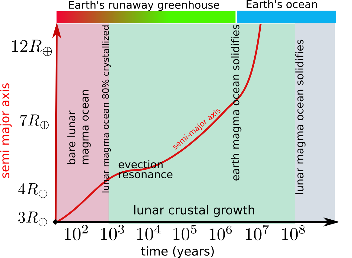
We summarize a rough timeline for events occurring during the formation and growth of the Moon’s crust, according to prevailing current understanding (see Figure 1). For more details on this timeline and alternate scenarios, see Ćuk and Stewart (2012); Zahnle et al. (2015); Ćuk et al. (2016); Tian et al. (2017). The ages of the oldest terrestrial and lunar zircons imply that the Earth’s surface must have cooled before crystallization of the lunar magma ocean was complete (Nemchin et al., 2009; Elkins-Tanton, 2012). Because of its water content, the Earth would have formed a thick greenhouse atmosphere a few thousand years after Moon formation (Zahnle et al., 2007; Sleep et al., 2014; Lupu et al., 2014; Zahnle et al., 2015). The optically thick atmosphere slows the cooling of the Earth and reduces its effective radiative temperature. The Moon is expected to have spun down into a spin synchronous or tidally locked state 1–100 years after formation (Garrick-Bethell et al., 2006, 2014).
For a few thousand years, the Earth’s radiative temperature would be a few hundred degrees higher than the effective temperature set by the Solar constant (see Figure 3 by Zahnle et al. 2015). During this time Earthshine could cause moderate heating on the Earth’s near side compared to the far side (Roy et al., 2014). Equations 2 and 3 by Roy et al. (2014) estimate the temperatures of the near and far sides of the Moon
| (1) | ||||
| (2) |
where are the distance to the Sun, and the radius and effective temperature of the Sun, are the distance of the Moon from the Earth, and the radius and effective temperature of the Earth. We estimate that at distance of and with the Earth’s radiative temperature at K, the near side of the Moon would be about K hotter than the far side. This is 4% of the Moon’s effective surface temperature of about K, set by the Solar constant.
The Earth’s greenhouse atmosphere lasts until the Earth’s magma ocean freezes, or a few million years after Moon formation (Zahnle et al., 2007; Sleep et al., 2014; Lupu et al., 2014; Zahnle et al., 2015). At this time the tidal dissipation rate in the Earth drops from to (Zahnle et al., 2015). A higher implies a slower drift rate of the Moon’s semi-major axis (Sleep et al., 2014; Zahnle et al., 2015). This scenario is called the ‘tethered Moon’ scenario. With such a high value of , coupled tidal evolution and thermal modeling imply that the Moon must solidify prior to reaching a semi-major axis of in order to maintain its orbital inclination going through the Cassini state transition at (Chen and Nimmo, 2016).
Touma and Wisdom (1998) showed that a resonance between perigee and perihelion, the evection resonance, could increase the Moon’s orbital eccentricity. The evection resonance occurs when the precession period of the Moon’s pericenter (due to torque from the oblate Earth) is equal to the Earth’s orbital period. The evection resonance location given by , the semi-major axis of the Moon’s orbit about the Earth, depends on the semi-major axis of the Earth’s orbit around the Sun, , and the Earth’s gravitational moment, . The resonance occurs where
| (3) |
where is the Earth’s mean motion in orbit about the Sun (center of mass of Earth/Moon binary), is the Moon’s mean motion about the Earth, and the mean radius of the Earth is . Touma and Wisdom (1998) estimated the location of the eviction resonance assuming that the Earth’s gravitational moment , proportional to the square of the Earth’s rotation rate. This assumption is consistent with a core and mantle hydrostatic model (Dermott, 1979). The resonance condition
| (4) |
where is the orbital semi-major axis of resonance. With the Earth’s rotation period of 5.2 hours, scaling from the Earth’s current gives a location for the resonance , as estimated by Touma and Wisdom (1998). However, if the Earth’s spin period is only 3 hours, as in a fast spinning Earth scenario (Ćuk and Stewart, 2012), the evection resonance is more distant, at .
If the Moon’s semi-major axis is drifting slowly, due to a high , capture into the evection resonance is assured, however the ratio of tidal heating parameters (known as the Mignard parameter) would limit the orbital eccentricity growth while in the evection resonance (Zahnle et al., 2015). A non-zero but low eccentricity might have been present when the Moon was near the Earth. The non-zero eccentricity allows the Moon to be tidally heated during this time. Zahnle et al. (2015) find that the eccentricity can grow to higher values when is between 20 and 40 due to the higher tidal dissipation in the Earth after it has solidified.
The Moon cannot coalesce within a semi-major axis of (Kokubo et al., 2000) equal to the Roche limit. The Roche limit is fairly large due to the higher mean density of Earth compared to that of the Moon. Because the evection resonance is located at a semi-major axis of only a few Earth radii, passage through evection resonance took place soon after Moon formation. Passage through evection resonance may also decrease the Moon’s semi-major axis (Tian et al., 2017; Touma and Wisdom, 1998). The evection resonance may have reduced the total angular momentum of the Earth-Moon system (Ćuk and Stewart, 2012). The Moon can escape the evection resonance if the tidal drift rate is fast enough to be non-adiabatic (Touma and Wisdom, 1998) or if tidal parameters (Love number and dissipation factor) vary and in this case the Moon could have passed through the resonance multiple times (Tian et al., 2017). Zahnle et al. (2015) estimate that the evection resonance is encountered sufficiently early that the Earth would be molten during the encounter. The Earth’s molten state implies that tidal dissipation in the Earth would be lower than estimated for a solid Earth giving slower orbital evolution (Zahnle et al., 2015). Thus tidal evolution could have taken place quite slowly in the vicinity of the evection resonance, and when the eccentricity was non-zero.
In summary, a magma ocean on the Earth may have reduced the drift rate in semi-major axis of the Moon, prolonging its passage through the evection resonance and allowing the lunar magma ocean to solidify when the Moon’s orbit was eccentric enough to be tidally heated and when the Moon was quite near the Earth.
1.2 Tidal heating when the Moon is near the Earth
In this paper we reconsider the notion that the lunar crust grew asymmetrically, rather than acquired its dichotomy after formation (as in the impact scenario by Jutzi and Asphaug 2011). In icy satellites with a crust decoupled from the mantle by a subsurface ocean, tidal dissipation in the crust is enhanced and can lead to global crustal thickness variations due to differences in the spatial distribution of tidal heating (Ojakangas and Stevenson, 1989; Tobie et al., 2003, 2005; Nimmo et al., 2007; Garrick-Bethell et al., 2010). In the absence of strong tidal heating, the equilibrium crustal thickness would be set by the equilibrium surface temperature, which varies as a function of latitude. This is ruled out by crustal thickness measurements, implying that additional processes, such as tidal heating must have affected crustal growth (Garrick-Bethell et al., 2010). Garrick-Bethell et al. (2010) proposed that degree 2 structure in the lunar highlands topography could be due to tidal heating that was enhanced near the poles.
Garrick-Bethell et al. (2010) computed the tidal heating rate using the quadrupole term in the expansion of the gravitational potential from the tidal perturber (here the Earth), as is commonly done because this term is the strongest (Kaula, 1964; Peale and Cassen, 1978). The gravitational potential of a point mass perturber (the Earth) of mass , raising a tide on a body (the Moon) of radius can be expanded in powers of , the distance between the two bodies, and spherical harmonics (Kaula, 1964; Peale and Cassen, 1978). Neglecting the angular dependence, the quadrupole term where is the gravitational constant. The next term in the expansion is the octupole term with . The relevant octupole spherical harmonic is lopsided with strength on the Moon’s near side opposite in sign to that on the far side. The octupole term arises because gravitational attraction from a perturber is stronger on the near side. The closer the perturber is to the body, the worse the quadrupole tidal approximation and the more important are higher order moment terms such as the octupole.
As the radius of a tidally heated body is usually small compared to its semi-major axis (for example the ratio of semi-major axis to radius for Io is 230 and that for Enceladus is 944), the octupole and higher order moments are usually neglected in tidal heating computations. An exception is Phobos, at only 2.76 Mars radii away from Mars, higher order terms are considered in modeling its tidal evolution (and drift rate in semi-major axis) due to tidal dissipation in Mars (rather than Phobos) (Bills. et al., 2005). If the Earth’s tidal dissipation parameter is large, to (corresponding to weak dissipation), while it hosted a magma ocean, as proposed by Zahnle et al. (2015), then lunar crustal growth could take place while the Moon’s semi-major axis was only . We explore the possibility that the octupole tidal perturbation could influence the tidal heating pattern during the era of lunar crustal growth, and cause a near/far side asymmetry.
Taking into account the body’s spin rate and the orbit variations, the tidal potential perturbation is expanded in a Fourier series where each term depends on a different frequency (e.g., equation 1 by Kaula 1964 and Peale and Cassen 1978). An elastic body is deformed by the tidal perturbation giving stress and strain tensors that are similarly expanded as a Fourier series with the same frequency spectrum. The strain tensor is computed from the displacement vector and with strain tensor components and displacement vector proportional to the potential perturbation (Love, 1944; Peale and Cassen, 1978). For the quadrupole potential tidal perturbation the strain tensor components
| (5) |
(equations 10–15 by Peale and Cassen 1978). Here is a unit-less Love number. Because these components are proportional to the potential term, the octupole term in the tidal perturbation induces a similar strain, but proportional to one higher power of ;
| (6) |
where is the Love number for the octupole perturbation term. The total strain is a sum of multipole terms and is sensitive to the angular dependence of each component (on spherical coordinate angles ).
Tidal dissipation, giving heat per unit volume, , is computed from the average over time of stress times strain rate
| (7) |
where both the stress and strain rate consist of a sum of terms (see equation 20 by Peale and Cassen 1978). Here the stress tensor is , the strain rate is , and the stress and strain are related by the shear modulus which can be a complex function, to take into account phase lag due to viscoelastic relaxation.
The strain rate depends on the strain times the tidal perturbation frequency. If the octupole term in the expansion is considered alone, we would expect the tidal heating rate to be times weaker than the classical tidal heating rate computed from the quadrupole term alone. However, the product of stress times strain rate contains equivalent frequency terms that are proportional to the product or and so are only a factor times weaker than the quadrupole tidal heating rate. The quadrupole heating pattern is symmetrical, heating the near and far sides of the Moon equivalently. However, inclusion of the octupole potential term in a computation of the heating rate would give a difference between near and far sides of order . This would give a 5–10% asymmetry in the tidal heating rate during the era of lunar crustal growth. An even larger asymmetry might be present as the ratio of maximum to minimum in the distribution of tidal heat could be larger than 1. With the quadrupole alone, the heat flux (heat per unit area) on the surface can vary by a factor of 2 (see for example, Beuthe 2013). Asymmetric tidal heating could be more important than a few percent difference in heat flux through the lunar crust due to Earth-shine (as we estimated in section 1.1).
1.3 Outline
The tidal dissipation rate inside the Moon has predominantly been predicted using a semi-analytical expansion method (e.g., Peale and Cassen 1978; Beuthe 2013, 2015). We use a numerical simulation technique instead. Because of their simplicity and speed, compared to more computationally intensive grid-based or finite element methods, mass-spring computations are a rough but straightforward method for simulating deformable bodies. By including spring damping forces they can model viscoelastic tidal deformation. Because all forces are applied between pairs of particles, angular momentum conservation is ensured. Extremely small strains can be precisely measured between two mass nodes so tidal deformation is measurable. We have previously used a mass-spring model to study tidal encounters (Quillen et al., 2016a), measure tidal spin down for spherical bodies over a range of viscoelastic relaxation timescales (Frouard et al., 2016), spin-down of triaxial bodies spinning about a principal body axis aligned with the orbit normal (Quillen et al., 2016b), obliquity evolution of minor satellites in the Pluto-Charon binary system (Quillen et al., 2017), excitation of normal modes and seismic waves on a non-spherical body (Quillen et al., 2019b) and dissipation in ellipsoids undergoing non-principal axis rotation (Quillen et al., 2019a).
In this study we use the mass spring models to track the distribution of tidally generated heat in a soft nearly spherical body, mimicking the Moon. The Moon is resolved with nodes and a spring network, and is in an eccentric orbit about its tidal perturber, here the Earth, that is modeled as a point mass. We measure the heat distribution from the dissipation rates in the springs. Tidal heating computations often assume spherically symmetric shell models for internal material properties such as density, composition, rigidity and viscosity (e.g., Peale and Cassen 1978; Ojakangas and Stevenson 1989; Tobie et al. 2005; Wahr et al. 2006; Nimmo et al. 2007; Wahr et al. 2009; Beuthe 2013, 2015). Our mass spring model simulations are not restricted to spherical symmetry.
We integrate the tidally generated heat giving a heat flux pattern as a function of latitude and longitude. Our simulated Moon has a dissipating shell, approximating a thin crust, on a soft interior, mimicking the lunar magma ocean. Our simulations are described in section 2. In section 3 we compare tidally generated heat distributions for a series of simulations with uniform crustal shell thickness that have different orbital semi-major axes. We examine the tidal heat distribution of a simulation with a crustal shell that has varying thickness. Models for asymmetric lunar crust growth are discussed in section 4. A summary and discussion follows in section 5.
2 Simulations
| Mean radius | 1737.1 km | |
|---|---|---|
| Mass | kg | |
| Mean density | 3344 kg m-3 | |
| Surface gravity | 1.62 m s-2 | |
| Equatorial surface temperature | 255∘ K | |
| Magma ocean temperature | 1175∘ C = K | |
| Crustal thermal conductivity | 1.8 W m | |
| Parameter for viscosity activation | 44 | |
| Latent heat of fusion in magma ocean | J/kg | |
| Density of plagioclase | 2670 kg m-3 | |
| Proportion of plagioclase in ocean | 0.2 |
Notes: In the second half of the table, the nominal value of is that used by Garrick-Bethell et al. (2010). The parameter for viscosity activity is discussed in section 4. The proportion is that used by Snyder et al. (1992); Warren (1986). The latent heat is the nominal value used by Tian et al. (2017).
| Minimum interparticle spacing | ||
| Maximum spring length | ||
| Number of nodes | ||
| Mass of a node | ||
| Number of springs | ||
| Length of a spring | ||
| Rest length of a spring | ||
| Spring constant (elastic) | ||
| Spring damping parameter | ||
| Strain of a spring | ||
| Energy dissipation rate of a spring | ||
| Simulation time step | ||
| Initial damping time | ||
| Total mass of resolved body | or | |
| Radius of resolved body | or | |
| Angular spin rate | ||
| Mass of perturber | or | |
| Orbital Eccentricity | ||
| Orbital semi-major axis | ||
| Orbital mean motion | ||
| Poisson ratio | ||
| Shear modulus | ||
| Viscosity | ||
| Viscoelastic relaxation time | ||
| Strain tensor | ||
| Stress tensor | ||
| Temperature | ||
| Heating rate per unit volume | ||
| Heat flux or heating rate per unit area | ||
| Crustal or shell thickness | ||
| Thermal conductivity | ||
| Latitude | ||
| Longitude | ||
| Coordinate for depth in crust | ||
| Tidal frequency | ||
| Hard/Soft Shell coupling parameter |
Notes: A subscript is put on a quantity at a mass node with index . Subscript refers to a spring connecting mass node to node . Subscripts for the stress and strain tensors refer to coordinate directions.
| Minimum interparticle distance | 0.11 | |
| Max spring length to min particle spacing | 2.3 | |
| Number of nodes | ||
| Number of springs per node | ||
| Spring constant in interior | ||
| Spring constant in shell | ||
| Damping parameter in interior | ||
| Damping parameter in shell | 1 | |
| Young’s modulus of interior | 1.3 | |
| Young’s modulus of shell | 7 | |
| Viscoelastic relaxation time in shell | 0.0015 | |
| Shell boundary equatorial radius | 0.7 | |
| Initial body spin | 0.5 | |
| Orbital eccentricity | 0.2 | |
| Time step | 0.005 | |
| Damping time | 20 | |
| Orbital period |
Notes: Due to variations in the generation of the random spring network, the number of springs per node and number of nodes varies from simulation to simulation; varies by about and varies by about . Additional simulation parameters are listed in Table 4.
| Simulation | M1 | M2 | M3 | M4 | O2 |
|---|---|---|---|---|---|
| 7 | 15 | 30 | 60 | 15 | |
| 2 | 4 | 8 | 16 | 4 | |
| Mass ratio | 81 | 813 | 6500 | 813 |
Notes: is the ratio of orbital semi-major axis to lunar radius. 3.7 times this represents the the semi-major axis in units of Earth radius. The M1–M4 simulations have spherical symmetry. The O2 simulation has an uneven crustal shell thickness. Additional simulation parameters are listed in Table 3.
To simulate tidal viscoelastic response of non-spherical bodies we use the mass-spring model (Quillen et al., 2016a; Frouard et al., 2016; Quillen et al., 2016b, 2017, 2019b) that is built on the modular N-body code rebound (Rein and Liu, 2012). An elastic solid is approximated as a collection of mass nodes that are connected by a network of massless springs. Springs between mass nodes are damped and so the spring network approximates the behavior of a Kelvin-Voigt viscoelastic solid with Poisson ratio of 1/4 (Kot et al., 2015).
The mass particles in the resolved spinning body are subjected to three types of forces: the gravitational forces acting on every pair of particles in the body and from external masses, and the elastic and damping spring forces acting only between sufficiently close particle pairs with previously identified springs connecting them. When a large number of particles is used to resolve the spinning body, the mass-spring model behaves like an isotropic continuum elastic solid (Kot et al., 2015; Kot and Nagahashi, 2016), including its ability to exhibit normal mode oscillations and transmit seismic waves (Quillen et al., 2019b). The Kelvin-Voigt model arises because spring forces are exerted in parallel with damping. The spring forces keep a self-gravitating body from collapsing. A Maxwell viscoelastic model, with spring and damper in series between pairs of massive particles, would collapse due to self-gravity. Symbols used to describe our simulations are summarized in Table 2.
The code has been checked by comparing simulated and predicted tidal heating rates for tidal spin down (Frouard et al., 2016) and by comparing simulated and predicted energy dissipation rates (wobble damping) for ellipsoids undergoing non-principal axis rotation (Quillen et al., 2019a). The code matches analytical predictions within 30%, even at low stress and strain. We attribute the discrepancies in the tidal spin down comparison to the neglect of bulk viscosity in the analytical calculation, not to a problem in the simulation technique. The differences between measured and predicted dissipation rates for wobble damping are the same size as differences between different two different analytical predictions and match these predictions over 4 orders of magnitude variation in the energy dissipation rate (Quillen et al., 2019a). We have also compared predictions using a quality factor (constant ) dissipation model, a Maxwell model and our simulations which obey a Kelvin-Voigt viscoelastic model (Quillen et al., 2019a). Sensitivity to numbers of particles simulated, spring network or lattice and particle generation technique is discussed by Quillen et al. (2016b). Normal mode frequencies and seismic wave propagation speeds were checked for a near-spherical shape model by Quillen et al. (2019b). We have also used this code to study spin-orbit resonance capture and crossing in multiple body systems (Quillen et al., 2017).
2.1 Sizes and units
Physical quantities are summarized in Table 1. Our simulations work with mass in units of , the mass of the resolved spinning body, here that of the Moon, and distances in units of volumetric radius, , the radius of a spherical body with the same volume. Here we take , the Moon’s mean equatorial radius. The ratio and we use this factor to compute the ratio of semi-major axis to Earth radius, .
For our mass-spring simulations it is convenient to work with time in units of a gravitational timescale
| (8) |
where on the last line we have used the mean density of the Moon, (listed in Table 1). It is helpful to define a unit of energy density
| (9) |
where we are using the Moon’s mass and mean radius . Pressure, energy density and elastic moduli are given in units of . The velocity of a massless particle in a circular orbit just grazing the surface of the body is , and the period of this orbit is .
2.2 Initial conditions
As done previously (Frouard et al., 2016), we consider two masses in orbit. One mass is the spinning body resolved with masses and springs. The other body, the tidal perturber, is a point mass with mass . The resolved body is the Moon, and the point mass perturber is the Earth. For our random spring model, particle or node positions for the resolved body are drawn from an isotropic uniform distribution but only accepted into the spring network if they are within the surface bounding a triaxial ellipsoid, , and if they are more distant than from every other previously generated particle. Particles nodes that are not inside the ellipsoid are deleted. Here are the body’s semi-major axes. For modeling the Moon we generate a spherical body with . Once the particle positions have been generated, every pair of particles within of each other are connected with a single spring. Springs are initiated at their rest lengths. Because of self-gravity the body is not exactly in hydrostatic equilibrium at the beginning of the simulation and the body initially vibrates. We apply additional damping at the beginning of the simulation for a time to remove these vibrations. Only after do we process simulation outputs for measurements of dissipation. After this time spring parameters are not varied.
The spherical resolved body is initially spinning at rate with spin axis aligned with the orbital angular momentum axis, and in an eccentric orbit about the point mass. As we are modeling a tidally locked Moon we start with spin with , the orbital mean motion. Here and are the orbital semi-major axis and eccentricity.
2.3 Energy Dissipation in the Mass-Spring model
We describe how we use the mass spring model simulations to track the energy dissipation in each spring. We consider a spring between two particles with coordinate positions , . The vector between the particles gives a spring length that we compare with the spring rest length . The spring strain is
| (10) |
The strain rate of a spring with length is
| (11) |
The elastic force on particle by the spring connecting is
| (12) |
with the spring constant and the unit vector . Our damping force on particle is proportional to the strain rate
| (13) |
with damping coefficient that is equivalent to the inverse of a damping time scale. Here is the reduced mass . The elastic and damping forces on particle have the opposite sign as in equations 12 and 13.
Taking the sum of damping force times velocity for both masses we find the energy dissipation rate in a single spring connecting node to is
| (14) |
At each time step of a simulation, we record for every spring. In a frame rotating with the body we average the tidal power per unit volume taking values of for each spring over a series of time steps. The mid-point of the spring is used to identify the location of generated heat. By counting the number of springs per unit volume and measuring their dissipation rate we create 3-dimensional internal maps of the tidal heating rate per unit volume.
2.4 Viscous relaxation time
We summarize the relation between the springs in the model and the approximated continuum material (following Kot et al. 2015; Quillen et al. 2016a; Frouard et al. 2016). Taking the continuum limit, the static Young’s modulus for the random mass spring model is computed from a sum over springs within a volume (Kot et al., 2015)
| (15) |
where is the rest length of a spring connecting node to node and is the spring constant of that spring. This equation expresses how a network with stronger springs and more springs per unit volume would give a stronger material. The shear modulus is
| (16) |
where the Poisson ratio for the random spring model.
The shear viscosity is similarly computed (Quillen et al., 2016a; Frouard et al., 2016) from a sum over springs within a volume
| (17) |
giving a relaxation time
| (18) |
Equation 17 expresses how a network with more heavily damped springs mimic a higher viscosity material. With nodes of the same mass, , and springs with the same damping parameter and spring constant , the viscoelastic relaxation time
| (19) |
where the factor 2 arises because we have used the reduced mass in equation 13.
We use a two layer model with properties in the interior denoted with subscript and those in the outer shell denoted with subscript , giving moduli , viscosities and relaxation timescales .
A body in spin synchronous or tidally locked state has tidal frequency the mean motion. The tidal frequency in units of the relaxation time . For , the quality function, giving the torque and integrated energy dissipation, is (see section 2.3 by Frouard et al. 2016) . In our simulations we chose damping parameter so as to remain in the linear regime and approximately giving a constant time lag tidal dissipation model. The tidal quality factor as a function of frequency for the Kelvin-Voigt rheology is qualitatively similar to that of the Maxwell rheology (Frouard et al., 2016). Both rheologies have quality factor that is linear at low frequencies and both reach a peak near (Frouard et al., 2016). Because we remain in the linear regime, our simulated material should give a tidal heat distribution similar to that predicted by a Maxwell model and with the same frequency dependence.
2.5 Simulation parameters
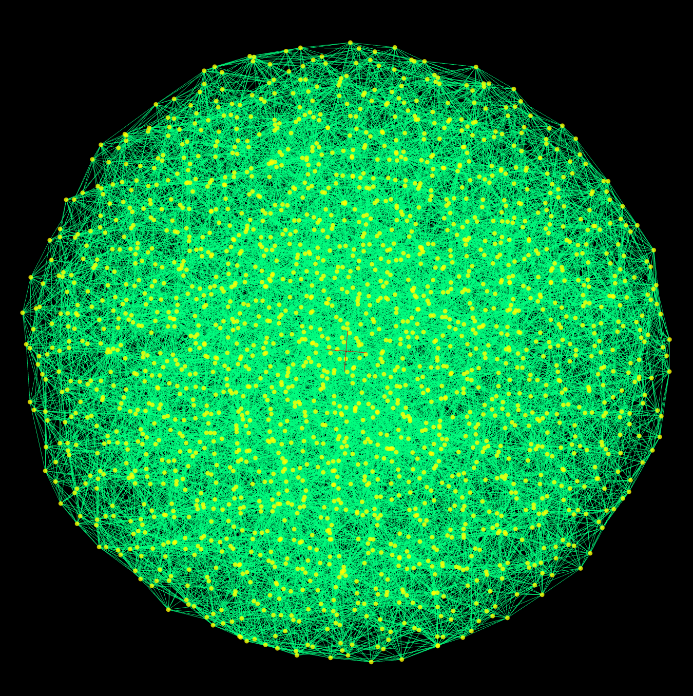
Common simulation parameters are listed in Table 3. A simulation visualization (a screen shot) showing the spring network from one of the simulation is shown in Figure 2. The resolved body is generated with mass nodes all identical in mass and is approximately uniform in mass density. Springs are generated with a two layer model. We use an ellipsoidal boundary to separate the crustal shell from the soft interior. Springs with midpoint inside this boundary have spring constants and damping parameter, , and those outside it, in the stiffer shell, are . The interior is adjusted to have a low damping coefficient, giving it a low dissipation rate. To mimic crustal heating we set the damping rate in the shell springs higher than that in the interior, . A low Young’s modulus is chosen for the interior to mimic a magma ocean. Our simulations do not model fluids and because the springs keep the body from collapsing due to self-gravity, we cannot simulate a material with Young’s modulus less than 1. A higher Young’s modulus is chosen for the shell, , to mimic the behavior of a stiffer but deformable elastic crust. The Young’s modulus for our simulation is in gravitational units, but for the Moon GPa (equation 9) so a modulus of 2 in gravitational units is similar to that of rock (80 GPa). Our simulations have a shell that is significantly harder than rock so that we can mimic the behavior of a hard shell on top of a softer interior.
We require accurate measurement of gravitational forces so that small variations in stresses and strains in the springs can be computed. As a result, we compute the gravitational forces between all pairs of particles during every time step and the the number of computations depends on the square of the number of mass nodes, (Quillen et al., 2016a; Frouard et al., 2016; Quillen et al., 2016b). The mean distance between mass nodes depends on , so a large increase in the number of nodes is required to increase the resolution of the simulation. The simulation time-step depends on the time for elastic waves to travel between mass nodes and so also scales with . Our simulations are not yet parallelized, so we cannot yet extend them to significantly larger numbers of nodes than a few thousand for simulations that are carried out for a few hundred orbital periods. The choice of run time depends upon which quantities we want to measure and their sensitivity to various oscillation frequencies (such as precession and libration).
We show five simulations, listed in Table 4 and with additional parameters in Table 3. Each has initial body spin in gravitational units and orbital mean motion , so the body starts in tidal lock (a spin synchronous state). The simulations each have a different semi-major axis. So that all simulations have the same body spin and the same orbital period, the mass of the perturber is adjusted so that the mean motion , (here is in units of ) giving larger perturber masses at larger orbital semi-major axes. The tidal heating rate is proportional to the mass of the perturber, however, the distribution of heat is not dependent on the perturber mass. We opted to adjust the perturber mass rather than the orbital frequency so we could fix the tidal frequency and viscoelastic relaxation time.
By varying the ratio of semi-major axis to body radius we can look at how proximity affects the tidal heating distribution. The orbital eccentricities for our simulations is 0.2. The tidal heating rate increases with eccentricity, however the predicted pattern of tidal heating as a function of latitude and longitude is not dependent on it (Peale and Cassen, 1978). We checked that the normalized heating distributions in our simulations are insensitive to orbital eccentricity.
The simulations M1, M2, M3, and M4 have spherical, uniform thickness crustal shells with inner radius but differing orbital semi-major axes. The simulation O2 has an asymmetric crustal shell and its orbital semi-major axis is the same as the M2 simulation. The shell boundary for this simulation is described with an ellipsoid
| (20) |
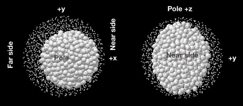
with positive initially toward the perturber and the axis pointing toward a pole. The O2 simulation has shell boundary equatorial radius , polar semi-axis and offset so that the shell is thinner at the poles and on the near side. By enlarging the rendered radii of the interior mass nodes we show in Figure 3 the shape of the shell with polar and equatorial views.
Due to the uneven particle distribution in the resolved body the initial body spin vector differs slightly from the desired value and the body spin axis is not exactly aligned with its principal body axes. Our simulations are not initially exactly at the lowest spin energy state and the body can oscillate about the spin synchronous state. This oscillation is sometimes called free libration. We don’t yet know how to set the initial conditions accurately enough to minimize the free libration amplitude. The time for an amplitude in free libration to die away is long as the libration frequency is slow for a nearly homogeneous sphere in a near spin synchronous state. We attempt to set the initial spin so that the initial obliquity is zero, however, the uneven particle distribution causes the spin vector to be slightly misaligned with principal body axes giving slow body precession. Longer simulations often showed true polar wander. We mitigate these problems with a high initial damping rate in the shell and by only running the simulations for 15 orbital periods afterward.
3 The spatial distribution of tidally generated heat
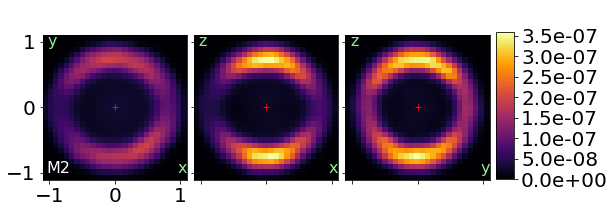
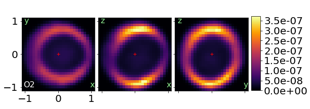
The distribution of tidally generated heat per unit volume on three planes that bisect the body are shown in Figure 4 for simulations M2 and O2 with parameters listed in Tables 3 and 4. In Figure 4 the positive axis points toward the perturber (the Earth) so is the Moon’s near side. The axis is aligned with spin axis and is perpendicular to the orbital plane, giving the poles. Positive corresponds to trailing side in the orbital plane (away from the direction of rotation). The Moon’s equator is in the plane. Units of energy dissipation per unit volume, , are gravitational or . The heating rate is measured from a sum of dissipation rates in the individual springs, but only springs near the bisecting plane and with midpoints within the pixel are summed. To decrease the sensitivity of the heat maps to node positions, we weight the sum with a Gaussian weight that depends on distance from the bisecting plane and has a dispersion of 0.2 in units of radius. The resulting weighted heat distribution for three bisecting planes and for two simulations is shown in Figure 4.
The heat distributions in the center and right panels of Figure 4 show that the heat per unit volume is highest at the poles. This is expected for a tidally locked body that is librating in an eccentric orbit (Peale and Cassen, 1978; Ojakangas and Stevenson, 1989; Tobie et al., 2005; Beuthe, 2013, 2015). Tidal heating is low in the interior because the springs there are only weakly damped. Because the tidal stress is higher at the base of the shell, the heating rate is higher at the shell base than near the surface; this too is predicted from semi-analytical tidal heating models (Peale and Cassen, 1978; Garrick-Bethell et al., 2010; Tobie et al., 2005; Beuthe, 2013, 2015).
In the O2 simulation (shown in the bottom row of panels in Figure 4), the shell is thinner at the poles and on the near side. The thickness of the far side shell is evident in the heat distribution in the equatorial plane shown in the leftmost panel. The heating pattern is similar to the M2 simulation even though the heat distribution appears oval for the right two panels because the core is extended in the direction. The heat distribution is a tilted oval because the body has not remained oriented so that it is aligned with the orbit and with the direction of the perturber.
The panels on the left, show heating in the equatorial plane. In the M2 simulations, there is a weak asymmetry, with the near side (positive ) somewhat hotter than the far side. The asymmetry can also be seen in the middle panel as the polar heating pattern is slightly warmer on the near side. We attribute the asymmetry to the proximity of the tidal perturber, making the octupole moment in the gravitational potential from the perturber strong enough to cause asymmetry in the heating rate. We discuss this asymmetry in more detail below.
3.1 Tidal heat distribution as a function of latitude and longitude
Tidal heating rate integrated from the heating rate per unit volume along radial rays and as a function of latitude and longitude are shown in Figure 5 for the same simulations we displayed in Figure 4. As heating may be asymmetric we show the entire range of longitude . Longitude corresponds to the near side, facing the Earth, whereas corresponds to the far side. Latitude is at the poles and zero at the equator. Our axis extends past on the right so that the far side can be examined. The region with on the right is the same as the region on the left with . Our plots differ from many studies that plot a restricted range with longitude because of the expected symmetry. Usually tidal heating from the quadrupole potential term significantly dominates over the octupole term. Heat maps in Figure 5 are normalized so that the average heating rate, computed from integrating over the surface, is equal to 1.
In Figure 5 we show on the lower right panel the heat pattern predicted with the thin shell model by Beuthe (2013). We have computed the tidal heating rate per unit area for eccentricity tides using associated Legendre polynomials, the function, equations 34, 36, and the coefficients in Table 1 by Beuthe (2013). The heat pattern in our simulations with larger semi-major axis (the M3,M4 simulations) resembles that predicted for thin shells (e.g., Peale and Cassen 1978; Ojakangas and Stevenson 1989; Tobie et al. 2005; Beuthe 2013) though the contrast between pole and equator is somewhat larger than in the predicted heat map. We attribute the difference to the coarseness of our simulation (numbers of mass nodes) and to a free libration amplitude in the simulation that is not present in the predicted heat distribution. The correspondence between predicted and numerically predicted heat maps demonstrates that the mass/spring model can match tidally generated internal heat distributions.
Figure 5 shows simulations that have the same spin and orbital periods. However the perturber mass and semi-major axes differ in the M1–M4 simulations. For the more distant perturbers (M3, M4 simulations), the tidal heating pattern is symmetric between near and far sides and resembles the heat flux distribution predicted for a thin shell and eccentricity tides. However, the heating pattern for the near and far sides differ for a closer perturber (the M1 and M2 simulations). The ratio of the heat flux on near and far sides is about for the M2 simulation with ratio of semi-major axis to body radius , corresponding to (using ). In section 1.2 we estimated that an octupole tidal heating term would be smaller than that of the dominant quadrupole by a factor of or 7% for the M2 simulation. The contrast in the quadrupole heat distribution exceeds 2 so a somewhat larger contrast than 7% is not necessarily unexpected.
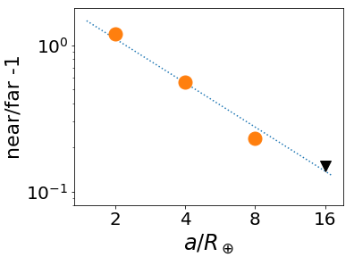
In Figure 6 we plot the ratio of near to far side heat flux subtracted by 1, , against orbital semi-major axis for the M1–M4 simulations as a function of semi-major axis ratio, . These are measured from averages of the heat maps in Figure 5 in regions centered at latitude 0 and longitudes and . The blue dotted line in the plot is a linear relation . We plot an upper limit for the M4 simulation. Comparison between M1–M4 simulations shows that the ratio of near and far side heat flux subtracted by 1 decreases approximately linearly as a function of inverse semi-major axis, or . This is consistent with our expectation that the asymmetry in heating arises from the octupole tidal term, as discussed in section 1.2. We attribute the near/far side asymmetry in the tidal heating distributions in the M1 and M2 simulations to the proximity of the Earth.
3.2 Tidal heat distribution in a shell with uneven thickness
The lower left panel in Figure 5 shows the O2 simulation that has an uneven thickness shell. Despite the extreme variations in shell thickness (see Figure 3), the distribution of tidal heat flux integrated radially through the shell resembles that of the other simulations. This surprised us as we had expected the heating rates per unit volume to be similar. We show only a single lopsided shell simulation here, however we found that simulations with different shaped shell boundaries and radial offsets and shell strengths exhibited similar behavior. We find that the heat flux, or heat per unit area integrated through the shell, as a function of latitude and longitude, is insensitive to shell thickness variations and is approximately proportional to the same function computed for a uniform thickness shell.
Recent analytical studies of elastic shells with variable thickness predict a phenomenon called stress amplification where stress is inversely proportional to the shell thickness (Behounkova et al., 2017; Beuthe, 2018). Physically, thinner and weaker areas of the shell deform and dissipate more than thicker areas which are stiffer. The insensitivity of our simulated tidal heat distribution to shell thickness is consistent with this behavior.
For body with a crust or shell over a subsurface ocean, a coupling parameter, , is used to classify systems as being in a ‘hard-shell’ or ‘soft-shell’ limit (e.g., Goldreich and Mitchell 2010; Beuthe 2018). Following equation 72 by Beuthe (2018),
| (21) |
with mean shell thickness, the surface gravitational acceleration and as defined in Equation 9. With a body is said to be in a hard-shell limit, with Enceladus having a hard shell due to its small size, but Ganymede, Europa (A et al., 2014) and the Moon when it had a magma ocean, in the soft-shell regime. The parameter increases with radius, putting larger bodies with thin shells or crusts in the soft-shell regime. The stress amplification phenomenon is predicted for hard shells, such as Enceladus, and in these the deformation of the surface depends on the depth integrated shear modulus and the surface stresses are inversely dependent on depth (Beuthe, 2018).
Our O2 simulation with thickness ratio and has and is in the hard-shell regime. However during lunar magma ocean solidification, the Moon, with GPa and crustal thickness 1 – 2%, has , and would have been in the soft-shell regime. We attempted to run simulations with thinner and softer shells, (so as to mimic the lunar crust). However, because the springs themselves keep the simulated body from collapsing from self-gravity, we are limited to materials with Young’s modulus . To decrease the shell thickness we would require more particles and shorter springs. As the number of particles is proportional to the mean inter-particle spacing to the third power, a significant reduction in shell thickness pushes us out of the realm of our code’s current capabilities (set primarily by the order direct gravity computation). Springs not only connect shell nodes to shell nodes and core nodes to core nodes, but also connect shell nodes to core nodes. Our simulated shell base cannot slide on top of the core. Even if we were able to simulate thin shells, the simulated body would not be consistent with hard shell floating on an ocean.
Previous computations of tidal heating in bodies that have a shell over an internal ocean (such as Europa or Enceladus) often assume a constant shell thickness when computing the heating rate per unit volume (e.g., Peale and Cassen 1978; Ojakangas and Stevenson 1989; Tobie et al. 2005; Wahr et al. 2006; Nimmo et al. 2007; Wahr et al. 2009; Beuthe 2013, 2015). This gives a pattern for the spatial heat distribution as a function of latitude and longitude or a function for the tidally generated heat per unit area as a function of latitude and longitude . Many studies necessarily have adopted the simple (but incorrect) assumption that , the tidal heating rate per unit volume, follows the same spatial distribution in latitude and longitude as the that is predicted from a constant thickness shell model. Then viscoelastic tidal heat with a temperature dependent viscosity is assumed when computing the temperature profile through a conductive crust. The result is a crust or shell thickness as a function of latitude and longitude that is consistent with the depth dependent tidal heating and the basal heat flux from the subsurface ocean (e.g., Ojakangas and Stevenson 1989; Tobie et al. 2005; Wahr et al. 2006; Nimmo et al. 2007; Wahr et al. 2009) but not necessarily with the elasticity of a variable thickness shell.
For soft shells, radial displacements due to tidal perturbation are set by the subsurface ocean and are insensitive to shell thickness, however latitude and longitude dependent stress functions are still dependent on shell thickness (see Beuthe 2018; section 5.2.4). Is the soft shell regime consistent with tidal heating rate per unit volume proportional to the tidal heating pattern predicted with a uniform thickness shell? The shell must stretch and slide over an ocean surface that is a gravitational equipotential surface. We would guess that an integral of the total elastic energy in the shell would be minimized. Taking only the stress and strain components tangential to the shell, the total elastic energy in the shell integrated over its volume , where the integral on the right is over solid angle. To minimize the total elastic energy from tidal deformation, stress and strain would tend to be lower where the shell is thickest. We lack simple analytical solutions and can’t yet extend our simulations to cover the soft-shell regime, however we suspect that in this regime too, the tidal heat distribution should depend on shell thickness and would be reduced in thicker regions.
The insensitivity to thickness variations, exhibited by our simulations and predicted for the hard-shell regime, gives a constraint on the tidally generated heat per unit volume;
| (22) |
where the function on the left is the heating pattern for of a uniform thickness shell and the integral on the right is a function of depth in the shell. The shell surface is at and the shell base is set by the shell thickness as a function of latitude and longitude. If the heating rate per unit volume is proportional to then a region with a thicker crust experiences more tidal heating. The crust cannot continue to grow as its base then would start to melt. However, if the heating rate per unit area is proportional to then thicker regions are cooler. The crust in a cool region, such as on the far side of the Moon, can continue to grow.
In summary, our simulations show that when the Moon was within a few Earth radii of the Earth, eccentricity tides are asymmetric, with the far side experiencing less heating than the near side and poles. Simulations with perturbers at different orbital semi-major axes illustrate that the asymmetry is dependent on the distance between the Earth and the Moon. The size of the asymmetry is approximately consistent with that estimated from the ratio of the octupole gravitational component of the perturber to the quadrupole component. A simulation with a variable shell thickness surprisingly showed a similar heating pattern to one with a uniform thickness shell. The insensitivity of the tidal heat flux to shell thickness implies that thicker areas of a shell deform less than thinner regions, a phenomena dubbed stress amplification by Beuthe (2018). This phenomena is predicted for a hard-shell regime and our simulations also lie in this regime, however the lunar crust during the epoch of magma ocean solidification is in a soft-shell regime. We lack predictions for the sensitivity of heating distributions to thickness (though see Beuthe 2018) and the ability to simulate in the soft-shell regime, but we suspect that here too crustal thickness variations would affect the tidal heating rate, with thicker regions less strongly tidally heated. With both asymmetric heating and tidal heating rate per unit area insensitive to crustal thickness, the lunar far side might form a thicker crust which could continue to grow. The asymmetry would persist as long as the Moon remains near the Earth and the octupole moment is strong, and would rapidly diminish as the Moon recedes from the Earth.
4 A tidally heated and conductive crustal lid
The asymmetry in the tidal heat flux between lunar near and far sides seen in our simulation ranges between 10– 50% (expressed as a ratio in nearside to farside heat flux). Can this weak asymmetry contribute to uneven lunar crustal growth? A thermal model was used by Garrick-Bethell et al. (2010) to account for the thinner polar lunar crust compared to the far side equatorial value with a latitude dependent tidal heating distribution. We extend their model to take into account asymmetric tidal heating. Parameters for our thermal models are listed in Table 1 and additional symbols and nomenclature are listed in Table 2. For the temperature at the lunar crust base, we take a magma ocean temperature of C, typical of solidus (and following Garrick-Bethell et al. 2010) and a surface temperature of K (typical of the lunar equator and following Vasavada et al. 1999).
We assume that the crust is in conductive thermal equilibrium with tidal heating in the crust and the basal heat flux into the crust from the top of the lunar magma ocean. We neglect radiogenic heating, as it is probably not an important contributor to the heat budget during the early evolution of the Moon (see section 2 by Tian et al. 2017, or the supplemental discussion by Garrick-Bethell et al. 2010). The time independent conductive heat diffusion equation for the crust
| (23) |
where is the tidal heating rate per unit volume. The tidal heating rate should be a function of latitude, longitude and temperature. Here is the thermal conductivity which we assume is independent of temperature, , or depth, . Following Garrick-Bethell et al. (2010) we adopt a conductivity of . This value is an average of conductivity for feldspar rich plutonic rocks including anorthsite over the temperature range of C (Clauser and Huenges, 1995).
The basal and surface heat fluxes
| (24) | ||||
| (25) |
The integrated tidal heat flux
| (26) |
Following previous studies (Ojakangas and Stevenson, 1989; Nimmo et al., 2007; Garrick-Bethell et al., 2010), rather than adopt an Arrhenius relationship for the temperature dependence of the viscosity, we instead use the simplified Frank-Kamenetski approximation (e.g., Solomatov 1995);
| (27) |
where is the reference viscosity at the crust base (at temperature ) and , where is an activation energy and is the gas constant. The viscosity is high at low temperature and reaches a minimum of at the crustal base with temperature equal to that of the well-mixed magma ocean. Using (a value for dry anorthsite; Rybacki and Dresen 2000) and gas constant (the nominal values from table S2 by Garrick-Bethell et al. 2010), we compute . With a Maxwell viscoelastic model and a viscosity estimated for the lunar crust, the viscoelastic relaxation time is long compared to the tidal oscillation period. In this limit, , the tidal energy dissipation rate per unit volume and is maximum at the crust base. With the viscosity following equation 27, the tidally generated heat per unit volume obeys
| (28) |
where is the maximum value at the crust base.
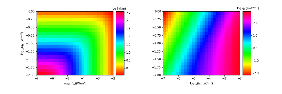
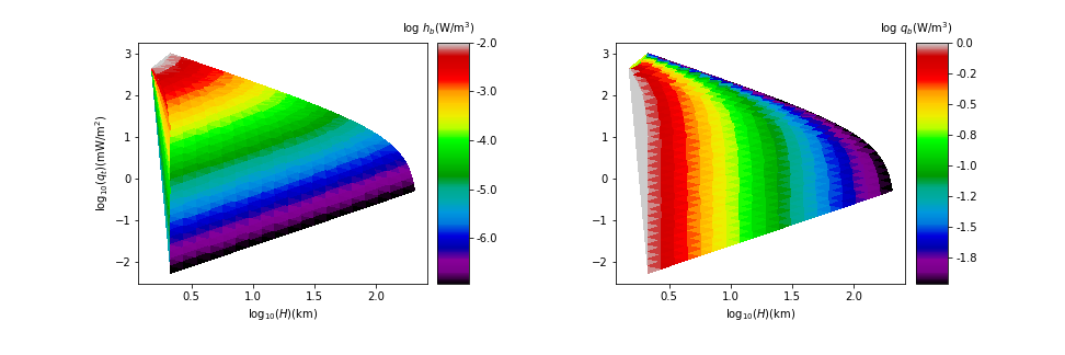
With an initial basal heat flux at temperature and basal tidal heating rate per unit volume we integrate the 1 dimensional conductive heat diffusion equation 23 upward in until the temperature reaches the surface temperature . We measure the crustal thickness and integrated tidal flux using equation 26. We repeat this procedure for a grid of and values. We show in the top panels of Figure 7 crustal thicknesses (top left, in km) and tidal flux (top right, in W/m2) computed from these 1-dimensional integrations. The bottom two panels in Figure 7 were constructed via triangulation from the points shown in the top two panels. The points shown in the bottom two panels were then used to construct smooth interpolation functions giving and . We use these functions to estimate the basal heat flux and basal tidal heat per unit volume given a particular crustal thickness and integrated tidally heat flux .
The left hand side of the top left panel in Figure 7 shows that at low levels of tidal heating, the crustal thickness depends inversely on the basal heat flux. This is expected for a conductive crust with no additional heating as a high heat flux gives a high temperature gradient. At higher levels of tidal heating, the crustal thickness is reduced because the tidal heat flux adds to the basal heat flux giving a higher heat flux through the crust. The top right panel shows that higher level of basal tidal heating and higher level of tidal heating integrated through the shell, (lower right on the top right panel) reduce the basal heat flux. The tidal heating acts like a blanket, preventing the magma ocean from cooling.
An interesting region in the lower right panel of Figure 7 is at = 10 km and at high tidal heat flux. The basal heat flux is quite sensitive to the level of tidal heating. Small variations in the tidal heating pattern could cause significant variations in the basal heat flux and so on the rate of magma ocean crystallization below the crust.
4.1 Estimates for crustal thickness variations
We can estimate the growth rate of the crust with
| (29) |
The factor is the proportion of plagioclase in the solidified portion of the melt. We assume (Snyder et al., 1992; Warren, 1986) and adopt a latent heat of J/kg for the magma ocean, following Tian et al. (2017) and a density of . We only allow crustal growth, and do not allow previously grown crust to melt.
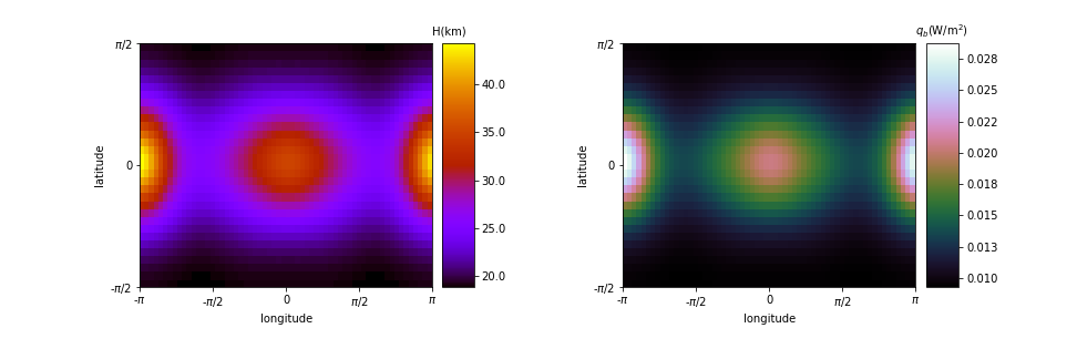
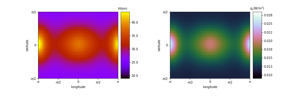
To estimate a crustal growth rate from a tidal heat distribution, we make some additional assumptions. Starting with km, we use either or to compute the basal heat flux . We assume that the local basal heat flux sets the local crustal growth rate, ignoring mixing in the magma ocean. The crustal thickness is updated using equation 29. The procedure is repeated, at each time step, updating the crustal thickness model. Each growth model is integrated for years with final crustal thickness distribution and basal heat flux at the end of the integration shown in the left and right panels of Figure 8. The basal heat flux maps resembles the crustal thickness maps. With higher basal heat flux beneath the lunar far side, the magma ocean preferentially crystallizes below the moon’s far side.
In our first growth model, shown in the top two panels of Figure 8, we assume that the distribution of tidal heating rate per unit area follows a pattern similar to those seen in our simulations. To match our asymmetric heating distribution we start with the heat distribution for a thin shell and eccentricity tide by Beuthe (2013) and shown in the lower right panel of Figure 4. To this we add a term to match the near and far side asymmetry we saw in our M2 simulation. We assume that follows this distribution, even though we allow the viscosity in the crust to depend on temperature. We assume that the average (over the sphere) tidal heating flux is mW m-2 and is constant in time. From and we use our interpolation function to compute the basal heat flux as a function of latitude and longitude.
In our second growth model, shown in the top two panels of Figure 8, we assume that the tidal heating rate per unit volume at the crust base, , follows the tidal heating pattern seen in our simulations. This and the crustal thickness as a function of latitude and longitude are used to compute the basal heat flux , and the crust thickness increased using that value. For this model we use a constant tidal heat per unit volume at the crust base of .
We found that the growth models were insensitive to the actual value used for . We have neglected surface temperature variations, though the poles could be cooler than the equator (Vasavada et al., 1999) and this could increase the thickness of the crust at the poles.
The model based on a tidal heat per unit area or distribution gives a moderate crustal asymmetry with thickness km on the near side and 44 km on the far side. The thickness variations are larger for this model than for that based on the tidal heating rate per unit volume at the crust base or distribution, with a similar far side thickness but a thicker near side at about 38 km. We also explored a heating model with and with the same heat pattern, with a result similar to the constant model.
In these models we have maintained a constant rate of asymmetric tidal heating throughout crustal growth. Once the Earth’s magma ocean solidifies, the semi-major axis of the Moon can more rapidly increase. The orbital eccentricity can grow, so tidal heating could continue to be important (see Zahnle et al. 2015), however tidal heating would no longer be asymmetric. We explored removing the heating asymmetry at different times in the first growth model (based on ) finding that a moderate crustal thickness asymmetry persists when the transition to quadrupolar heating takes place at greater than 40 Myr and is completely absent if the transition takes place earlier than 20 Myr. This time for crustal asymmetry to persist exceeds the time when Earth’s magma ocean solidifies, which is at most 6 Myr (Zahnle et al., 2015) and when the Moon would start to more rapidly drift away from the Earth. Our simple crustal models predict that the asymmetry is wiped out once the tidal heating becomes entirely quadrupolar.
In summary, simple heat conductivity and crustal growth models show that a moderate crustal asymmetry could persist during crustal growth, and if the thicker parts of the crust deform less than the thinner parts, the asymmetry would be larger. However, these simple heat conductivity models neglect mixing in the magma ocean and fail to match the extent of the observed lunar crustal thickness asymmetry. Moreover, the crustal thickness asymmetry fails to persist once the heating becomes entirely quadrupolar.
5 Summary and Discussion
Recent work on the early evolution of the Earth (Zahnle et al., 2007; Sleep et al., 2014; Lupu et al., 2014; Zahnle et al., 2015) have shown that a magma ocean on the Earth may have reduced the tidally induced drift rate of the Moon’s orbital semi-major axis. This prolongs the Moon’s passage through the evection resonance and allows the lunar magma ocean to partially slowly solidify when the Moon’s orbit was eccentric and when it was quite near the Earth.
We use a mass spring model viscoelastic code to model tidal heating of a spin synchronous Moon in eccentric orbit about the Earth. By tracking energy dissipation in the springs we measure the distribution of internally dissipated heat. We ran simulations of a spinning body with a dissipative shell, mimicking an elastic lunar crust, overlaying a softer interior with lower viscoelastic dissipation, mimicking a magma ocean. The distribution of tidally generated heat per unit area for perturbers at larger orbital semi-major axes resembles that predicted for eccentricity tides with a thin hard shell model (that by Beuthe 2013).
Our simulations show that when the Moon was within a few Earth radii of the Earth, eccentricity tides are asymmetric. The far side is less strongly heated than the near side and poles. The simulations show that the near/far side asymmetry decreases with increasing orbital semi-major axis, and the size of the asymmetry is consistent with that estimated from the ratio of the octupole gravitational component of the perturber to the quadrupole component. The asymmetry is due to the octupole component of the gravitational potential of the perturber. This term is only significant when the perturber is nearby, and is usually neglected from tidal heating computations as a consequence.
A simulation with a variable shell thickness surprisingly showed a similar heating pattern to one with an uniform thickness shell. The insensitivity of the tidal heat flux to shell thickness could arise when thicker areas of a shell deform less than thinner regions, a phenomena recently dubbed stress amplification by Beuthe (2018). Stress amplification is predicted for bodies, such as Enceladus, that lie in a hard-shell regime (Beuthe, 2018). During the epoch of lunar magma ocean solidification, the lunar crust would have been in a soft-shell regime. Unfortunately, we lack predictions for the sensitivity of heating distributions to thickness and the ability to simulate in the soft-shell regime, but we suspect that here too crustal thickness variations would affect the tidal heating rate, with thicker regions less strongly heated. Insensitivity of the heat flux distribution to thickness variations reduces the tidal heating rate in thicker crustal regions. With both asymmetric heating and tidal heating rate per unit area insensitive to crustal thickness, the lunar far side might form a stiff, thick and cool crust which could continue to grow.
We constructed thermal conductivity models for the lunar crust to take into account the distribution of tidal heating. We used an asymmetric heating pattern like those seen in our simulations as input to the crustal growth model. The local tidal heating rate affects the basal heat flux which we used to compute the local crustal growth rate. The basal heat flux sets the rate of magma ocean cooling and crystallization. The resulting models illustrated moderate crustal thickness variations after years of crustal growth, at a constant rate of tidal heating and with asymmetric tidal heating. Larger thickness variations were present at the end of crust growth for a tidal heating rate per unit area independent of crustal thickness variations, than with heating rate per unit volume independent of crustal thickness variations. However, thickness near/far side asymmetry did not persist in our simple models without asymmetric heating. Thus once the moon moves away from the Earth, following solidification of the Earth’s magma ocean, the crustal thickness near/far side asymmetry is not maintained. Because recent scenarios exhibit a range of possible orbital eccentricity and semi-major axis evolutionary paths, our models also neglect variation in the tidal heating rate. Thus we have not taken into account possible of episodes of melting or that most crustal growth could have taken place when the Moon was at larger semi-major axis.
Our crustal growth models also neglect mixing in the magma ocean and fail to match the extent of the observed lunar crustal thickness variations even if the tidal heating asymmetry is maintained. We assumed that the crust would grow where the basal heat flux was high. This makes the crust base akin to a refrigerated plate that is floating on ice-water, with ice more likely to collect on the most strongly cooled regions of the plate. However, the magma ocean in the cooler regions could also be more turbulent and this could prevent accumulation of floating plagioclase crystals (e.g., Tonks and Melosh 1990). Models of convection and crystal sedimentation in the lunar magma are complex (Snyder et al., 1992; Solomatov, 2000; Parmentier et al., 2002; Nemchin et al., 2009; Lavorel and LeBars, 2009; Ohtake et al., 2012; Laneuville et al., 2013; Charlier et al., 2018), but could in future explore sedimentation with uneven heat flux through the upper lunar magma ocean boundary.
The recent tidal heating models by Garrick-Bethell et al. (2014), estimate the lunar tidal heat flux for an eccentricity of – 0.03 and at a semi-major axis of (see their Table S13). Using the standard formula (e.g., equation 1 by Yoder and Peale 1981) the integrated tidal heating rate is proportional to . To achieve the same heating rate at a semi-major axis of as at 20 , the eccentricity must be 31 times lower, or in the range 0.0006 – 0.001. For lunar crustal growth to take place when the Moon was closer to the Earth, the orbital eccentricity must be substantially lower than adopted by recent models. With the tethered Moon scenario (Zahnle et al., 2015), the Moon does not acquire much eccentricity passing through the evection resonance. These models have not yet estimated a range of possible values. To estimate it, tidal evolution could be explored taking into account the degree of solidification and variations in the dissipation rates in both Earth and Moon.
Even if the early tidal heating asymmetry found here does not directly induce asymmetric crustal growth through variations in basal heat flux, it might serve as a trigger for continued asymmetric crustal growth. If crustal growth is unstable (as discussed by Garrick-Bethell et al. 2010), with thicker and stronger regions tending to grow faster, as suggested by the stress amplification scenario for hard-shells (Behounkova et al., 2017; Beuthe, 2018), then early asymmetric tidal heating might be amplified via later crustal growth, after tidal heating becomes predominantly quadrupolar. Alternatively, we could also conclude that an early episode of asymmetric tidal heating does not affect the later development of lunar crustal thickness variations.
We have explored the possibility that the distribution of tidal heating could affect the difference in near and far side lunar crust thickness. Our scenario is similar to that proposed to explain thinner crust at the poles by Garrick-Bethell et al. (2010), (also see Garrick-Bethell et al. 2014) however our model relies on proximity to the Earth as it depends on the strength of the Earth’s octupole gravitational potential term. Our mass spring simulations are not restricted to spherical symmetry and we used that flexibility to search for asymmetric heating and sensitivity of the tidal heating pattern to crustal thickness variations. The similarity between predicted and simulated heat flux distributions suggests that this type of simulation, if expanded, may become increasingly flexible and powerful. However, the simulations were difficult to adjust to minimize free libration, and we often saw unintended polar wander and spin precession. Currently our simulations only simulate Kelvin-Voigt viscoelastic solids with a Poisson ratio of 1/4 and we cannot yet simulate other rheologies, thinner crusts or hybrid models containing subsurface oceans.
Acknowledgements.
A.C. Quillen thanks L’Observatoire de la Côte d’Azur for their warm welcome and hospitality March and April 2018. This study was initiated with the help of Genn Shroeder. We thank Patrick Michel, Mark Wieczorek, Marco Delbo, Randal Nelson, Mohamed Zaghoo, Cynthia Ebinger, Jing Luan, Esteban Wright, and Alexander Gysi for helpful discussions.
A. C. Quillen is grateful for generous support from the Simons Foundation. This material is based upon work supported in part supported by NASA grant 80NSSC17K0771, National Science Foundation Grant No. PHY-1757062 and NASA grant NNX15AI46G (PGGURP) to PI Tracy Gregg.
Code used in this paper is available at https://github.com/aquillen/moon_heat .
Bibliography
References
- A et al. (2014) A, G., Wahr, J., Zhong, S., 2014. The effects of laterally varying icy shell structure on the tidal response of Ganymede and Europa. Journal of Geophysical Research Planets 119, 659–678.
- Abe (1997) Abe, Y., 1997. Thermal and chemical evolution of the terrestrial magma ocean. Physics of the Earth and Planetary Interiors 100, 27–39.
- Behounkova et al. (2017) Behounkova, M., Soucek, O., Hron, J., Cadek, O., 2017. Plume activity and tidal deformation on Enceladus influenced by faults and variable ice shell thickness. Astrobiology 17, 941–954.
- Beuthe (2013) Beuthe, M., 2013. Spatial patterns of tidal heating. Icarus 223, 308–329.
- Beuthe (2015) Beuthe, M., 2015. Tides on Europa: The membrane paradigm. Icarus 248, 109–134.
- Beuthe (2018) Beuthe, M., 2018. Enceladus’s crust as a non-uniform thin shell: I tidal deformations. Icarus 302, 145–174.
- Bills. et al. (2005) Bills., B.G., Neumann, G.A., Smith, D.E., Zuber, M.T., 2005. Improved estimate of tidal dissipation within Mars from MOLA observations of the shadow of phobos. Journal of Geophysical Research 110, E07004.
- Borg et al. (1999) Borg, L.E., Norman, M., Nyquist, L.E., Bogard, D., Synder, G., Taylor, L., Lindstrom, M., 1999. Isotopic studies of ferroan anorthosite 62236: A young lunar crustal rock from a light rare-earth-element-depleted source. Geochimica et Cosmochimica Acta 63, 2679–2691.
- Charlier et al. (2018) Charlier, B., Grove, T.L., Namur, O., Holtz, F., 2018. Crystallization of the lunar magma ocean and the primordial mantle-crust differentiation of the moon. Geochimica et Cosmochimica Acta 234, 50–69.
- Chen and Nimmo (2016) Chen, E.M.A., Nimmo, F., 2016. Tidal dissipation in the lunar magma ocean and its effect on the early evolution of the earth–moon system. Icarus 275, 132–142.
- Clauser and Huenges (1995) Clauser, C., Huenges, E., 1995. Thermal conductivity of rocks and minerals, in: Ahrens, T. (Ed.), Rock physics and phase relations: A handbook of physical constants. American Geophysical Union: Washington DC. volume 3 of AGU Reference Shelf Series.
- Ćuk et al. (2016) Ćuk, M., Hamilton, D.P., Lock, S., Stewart, S.T., 2016. Tidal evolution of the Moon from a high-obliquity, high-angular-momentum earth. Nature 537, 402–406.
- Ćuk and Stewart (2012) Ćuk, M., Stewart, S.T., 2012. Making the Moon from a fast-spinning Earth: A giant impact followed by resonant despinning. Science 338, 1047–1052.
- Dermott (1979) Dermott, S.F., 1979. Shapes and gravitational moments of satellites and asteroids. Icarus 37, 576–586.
- Elkins-Tanton (2012) Elkins-Tanton, L.T., 2012. Magma oceans in the inner solar system. Annual Review of Earth Planetary Sciences 40, 113–39.
- Elkins-Tanton et al. (2011) Elkins-Tanton, L.T., Burgess, S., Yin, Q.Z., 2011. The lunar magma ocean: Reconciling the solidification process with lunar petrology and geochronology. Earth and Planetary Science Letters 304, 326–336.
- Frouard et al. (2016) Frouard, J., Quillen, A.C., Efroimsky, M., Giannella, D., 2016. Numerical simulation of tidal evolution of a viscoelastic body modelled with a mass-spring network. Monthly Notices of the Royal Astronomical Society 458, 2890–2901.
- Garrick-Bethell et al. (2010) Garrick-Bethell, I., Nimmo, F., Wieczorek, M.A., 2010. Structure and formation of the lunar farside highlands. Science 330, 949–951.
- Garrick-Bethell et al. (2014) Garrick-Bethell, I., Perera, V., Nimmo, F., Zuber, M., 2014. The tidal-rotational shape of the Moon and evidence for polar wander. Nature 412, 181–184.
- Garrick-Bethell et al. (2006) Garrick-Bethell, I., Wisdom, J., Zuber, M., 2006. Evidence for a past high-eccentricity lunar orbit. Science 313, 652–655.
- Goldreich and Mitchell (2010) Goldreich, P.M., Mitchell, J.L., 2010. Elastic ice shells of synchronous moons: Implications for cracks on europa and non-synchronous rotation of titan. Icarus 209.
- Jutzi and Asphaug (2011) Jutzi, M., Asphaug, E., 2011. Forming the lunar farside highlands by accretion of a companion moon. Nature 476, 69–72.
- Kaula (1964) Kaula, M., 1964. Tidal dissipation by solid friction and the resulting orbital evolution. Reviews of Geophysics 2, 661–684.
- Kokubo et al. (2000) Kokubo, E., Ida, S., Makino, J., 2000. Evolution of a circumterrestrial disk and formation of a single moon. Icarus 148, 419–436.
- Kot and Nagahashi (2016) Kot, M., Nagahashi, H., 2016. Mass spring models with adjustable poisson’s ratio. The Visual Computer 33, 283–291.
- Kot et al. (2015) Kot, M., Nagahashi, H., Szymczak, P., 2015. Elastic moduli of simple mass spring models. The Visual Computer: International Journal of Computer Graphics 31, 1339–1350.
- Laneuville et al. (2013) Laneuville, M., Wieczorek, M.A., Breuer, D., Tosi, N., 2013. Asymmetric thermal evolution of the Moon. Journal of Geophysical Research: Planets 118, 1435–1452.
- Lavorel and LeBars (2009) Lavorel, G., LeBars, M., 2009. Sedimentation of particles in a vigorously convecting fluid. Physics Review E 80, 046324.
- Loper and Werner (2002) Loper, D.E., Werner, C.L., 2002. On lunar asymmetries 1. Tilted convection and crustal asymmetry. J. Geophysics Research 107, 5046.
- Love (1944) Love, A.E.H., 1944. A Treatise on the Mathematical Theory of Elasticity. 4th ed., Dover, New York.
- Lupu et al. (2014) Lupu, R.E., Zahnle, J., Marley, M.S., Schaefer, L., Fegley, B., Morley, C., Cahoy, K., Freedam, R., Fortney, J., 2014. The atmospheres of earthlike planets after giant impact events. Astrophysical Journal 784, 27–46.
- McCallum (2001) McCallum, I.S., 2001. A new view of the Moon in light of data from Clementine and Prospector missions. Earth Moon and Planets 85-86, 253–269.
- Meyer et al. (2010) Meyer, J., Elkins-Tanton, L., Wisdom, J., 2010. Coupled thermal–orbital evolution of the early Moon. Icarus 208, 1–10.
- Nemchin et al. (2009) Nemchin, A., Timms, N., Pidgeon, R., Geisler, T., Reddy, S., Meyer, C., 2009. Timing of crystallization of the lunar magma ocean constrained by the oldest zircon. Nature geoscience 2, 133–136.
- Nimmo et al. (2007) Nimmo, F., Thomas, P.C., Pappalardo, R.T., Moore, W.B., 2007. The global shape of Europa: Constraints on lateral shell thickness variations. Icarus 191, 183–192.
- Ohtake et al. (2012) Ohtake, M., Takeda, H., Matsunaga, T., Yokota, Y., Haruyama, J., Morota, T., Yamamoto, S., Ogawa, Y., andY. Karouji, T.H., Saiki, K., Lucey, P.G., 2012. Asymmetric crustal growth on the Moon indicated by primitive farside highland materials. Nature Geoscience 5, 384–388.
- Ojakangas and Stevenson (1989) Ojakangas, G.W., Stevenson, D., 1989. Thermal state of an ice shell on Europa. Icarus 81, 220–241.
- Parmentier et al. (2002) Parmentier, E.M., Zhong, S., Zuber, M., 2002. Gravitational differentiation due to initial chemical stratification: Origin of lunar asymmetry by the creep of dense kreep? Earth and Planetary Science Letters 201, 473–480.
- Peale and Cassen (1978) Peale, S.J., Cassen, P., 1978. Contribution of tidal dissipation to lunar thermal history. Icarus 36.
- Quillen et al. (2016a) Quillen, A.C., Giannella, D., Shaw, J.G., Ebinger, C., 2016a. Crustal failure on icy moons from a strong tidal encounter. Icarus 275, 267–280.
- Quillen et al. (2016b) Quillen, A.C., Kueter-Young, A., Frouard, J., Ragozzine, D., 2016b. Tidal spin down rates of homogeneous triaxial viscoelastic bodies. Monthly Notices of the Royal Astronomical Society 463, 1543–1553.
- Quillen et al. (2017) Quillen, A.C., Nichols-Fleming, F., Chen, Y.Y., Noyelles, B., 2017. Obliquity evolution of the minor satellites of Pluto and Charon. Icarus 293, 94–113.
- Quillen et al. (2019a) Quillen, A.C., Wagner, K.J., Sánchez, P., 2019a. Simulations of wobble damping in viscoelastic rotators. Monthly Notices of the Royal Astronomical Society 485, 725–738.
- Quillen et al. (2019b) Quillen, A.C., Zhao, Y., Chen, Y., Sanchez, P., Nelson, R.C., Schwartz, S.R., 2019b. Impact excitation of a seismic pulse and vibrational normal modes on asteroid Bennu and associated slumping of regolith. Icarus 319, 312–333.
- Rein and Liu (2012) Rein, H., Liu, S.F., 2012. REBOUND: an open-source multi-purpose n-body code for collisional dynamics. Astronomy and Astrophysics 537, A128.
- Roy et al. (2014) Roy, A., Wright, J.T., Siggurdson, S., 2014. Earthshine on a young moon: Explaining the lunear farside highlands. The Astrophysical Journal Letters 788, L42–44.
- Rybacki and Dresen (2000) Rybacki, E., Dresen, G., 2000. Dislocation and diffusion creep of synthetic anorthite aggregates. Journal of Geophysical Research: Solid Earth 105, 26017–26036.
- Shearer et al. (2006) Shearer, C.K., Hess, P.C., Wieczorek, M.A., Pritchard, M.E., Parmentier, E.M., Borg, L.E., Longhi, J., Elkins-Tanton, L.T., Neal, C.R., Antonenko, I., Canup, R.M., Halliday, A.N., Grove, T.L., Hager, B.H., Lee, D.C., Wiechert, U., 2006. Thermal and magmatic evolution of the Moon. Reviews in Mineralogy and Geochemistry 60, 365–518.
- Sleep et al. (2014) Sleep, N.M., Zahnle, K.Z., Lupu, R.E., 2014. Terrestrial aftermath of the Moon-forming impact. Philosophical Transactions Royal Society A 372, 20130172.
- Snyder et al. (1992) Snyder, G.A., Taylor, L.A., Neal, C.R., 1992. A chemical model for generating the sources of mare basalts: Combined equilibrium and fractional crystallization of the lunar magmasphere. Geochim. Cosmochim. Acta 56, 3809–3823.
- Solomatov (1995) Solomatov, V., 1995. Scaling of temperature-dependent and stress-dependent viscosity convection. Physics of Fluids 7, 266–274.
- Solomatov (2000) Solomatov, V.S., 2000. Fluid dynamics of a terrestrial magma ocean, in: Canup, R.M., Righter, K. (Eds.), Origin of the Earth and Moon, University of Arizona Press. pp. 323–338.
- Spera (1992) Spera, F.J., 1992. Lunar magma transport phenomena. Geochim. Cosmochim Acta 56, 2253–2266.
- Tian et al. (2017) Tian, Z., Elkins-Tanton, L., Wisdom, J., 2017. Coupled orbital-thermal evolution of the early Earth-Moon system with a fast-spinning earth. Icarus 281, 90–102.
- Tobie et al. (2003) Tobie, G., Choblet, G., Sotin, C., 2003. Tidally heated convection: Constraints on Europa’s ice shell thickness. Journal of Geophysical Research 108, 5124.
- Tobie et al. (2005) Tobie, G., Mocquet, A., Sotin, C., 2005. Tidal dissipation within large icy satellites: Applications to Europa and Titan. Icarus 177, 534–549.
- Tonks and Melosh (1990) Tonks, W.B., Melosh, H.J., 1990. The physics of crystal settling and suspension in a turbulent magma ocean, in: Newsom, H., Jones, J. (Eds.), Origin of the Earth, Oxford University Press. pp. 151–174.
- Touma and Wisdom (1998) Touma, J., Wisdom, J., 1998. Resonances in the early evolution of the Earth-Moon system. Astronomical Journal 115, 1653–1663.
- Vasavada et al. (1999) Vasavada, A.R., Paige, D.A., Wood, S.E., 1999. Near-surface temperatures on Mercury and the Moon and the stability of polar ice deposits. Icarus 141, 179–193.
- Wahr et al. (2009) Wahr, J., Selvans, Z.A., Mullen, M., Barr, A., Collins, G., Selvans, M., Pappalardo, R., 2009. Modeling stresses on satellites due to nonsynchronous rotation and orbital eccentricity using gravitational potential theory. Icarus 200, 188–206.
- Wahr et al. (2006) Wahr, J.M., Zuber, M.T., Smith, D.E., Lunine, J.I., 2006. Tides on Europa, and the thickness of Europa’s icy shell. Journal of Geophysical Research 111, E12005.
- Warren (1986) Warren, P.H., 1986. The bulk-Moon MgO/FeO ratio: A highlands perspective, in: Hartmann, W.K. (Ed.), Origin of the Moon, Lunar and Planetary Institute, Tucson, AZ. pp. 279–310.
- Wasson and Warren (1980) Wasson, J.T., Warren, P.H., 1980. Contribution of the mantle to the lunar asymmetry. Icarus 44, 752–771.
- Wieczorek et al. (2013) Wieczorek, M.A., Neumann, G.A., Nimmo, F., Kiefer, W.S., Taylor, G.J., Melosh, H.J., Phillips, R.J., Solomon, S.C., Andrews-Hanna, J.C., Asmar, S.W., Konopliv, A.S., Lemoine, F.G., Smith, D.E., Watkins, M.M., Williams, J.G., Zuber, M.T., 2013. The crust of the Moon as seen by GRAIL. Science 339, 671–675.
- Wood et al. (1970) Wood, J., Dickey, J., Marvin, U., Powell, B., 1970. Lunar anorthosites. Science 167, 602–604.
- Yoder and Peale (1981) Yoder, C.F., Peale, S.J., 1981. The tides of Io. Icarus 47, 1–37.
- Zahnle et al. (2007) Zahnle, K., Arndt, N., Cockell, C., Halliday, A., Nisbet, E., Selsis, F., Sleep, N.H., 2007. Emergence of a habitable planet. Space Sci. Rev. 129, 35–78.
- Zahnle et al. (2015) Zahnle, K.J., Lupu, R., Dobrovolskis, A., Sleep, N.H., 2015. The tethered Moon. Earth and Planetary Science Letters 427, 74–82.
- Zuber et al. (1994) Zuber, M.T., Smith, D.E., Lemoine, F.G., Neumann, G.A., 1994. The shape and internal structure of the Moon from the Clementine mission. Science 266, 1839–1843.