Abstract

Bilevel optimization has been recently revisited for designing and analyzing algorithms in hyperparameter tuning and meta learning tasks. However, due to its nested structure, evaluating exact gradients for high-dimensional problems is computationally challenging. One heuristic to circumvent this difficulty is to use the approximate gradient given by performing truncated back-propagation through the iterative optimization procedure that solves the lower-level problem. Although promising empirical performance has been reported, its theoretical properties are still unclear. In this paper, we analyze the properties of this family of approximate gradients and establish sufficient conditions for convergence. We validate this on several hyperparameter tuning and meta learning tasks. We find that optimization with the approximate gradient computed using few-step back-propagation often performs comparably to optimization with the exact gradient, while requiring far less memory and half the computation time.

1 INTRODUCTION

Bilevel optimization has been recently revisited as a theoretical framework for designing and analyzing algorithms for hyperparameter optimization [1] and meta learning [2]. Mathematically, these problems can be formulated as a stochastic optimization problem with an equality constraint (see Section 1.1):

$$\begin{split}\min_{\lambda}F(\lambda)&:=\mathbb{E}_{S}\left[f_{S}(\hat{w}_{S}^{*}(\lambda),\lambda)\right]\\[-3.0pt] \text{s.t.}\quad\hat{w}_{S}^{*}(\lambda)&\approx_{\lambda}\operatorname*{arg\,min}_{w}g_{S}(w,\lambda)\end{split}$$ (1)

where $w$ and $\lambda$ are the parameter and the hyperparameter, $F$ and $f_{S}$ are the expected and the sampled upper-level objective, $g_{S}$ is the sampled lower-level objective, and $S$ is a random variable called the context. The notation $\approx_{\lambda}$ means that $\hat{w}_{S}^{*}(\lambda)$ equals the unique return value of a prespecified iterative algorithm (e.g. gradient descent) that approximately finds a local minimum of $g_{S}$. This algorithm is part of the problem definition and can also be parametrized by $\lambda$ (e.g. step size). The motivation to explicitly consider the approximate solution $\hat{w}_{S}^{*}(\lambda)$ rather than an exact minimizer $w_{S}^{*}$ of $g_{S}$ is that $w_{S}^{*}$ is usually not available in closed form. This setup enables $\lambda$ to account for the imperfections of the lower-level optimization algorithm.

Solving the bilevel optimization problem in (1) is challenging due to the complicated dependency of the upper-level problem on $\lambda$ induced by $\hat{w}_{S}^{*}(\lambda)$. This difficulty is further aggravated when $\lambda$ and $w$ are high-dimensional, precluding the use of black-box optimization techniques such as grid/random search [3] and Bayesian optimization [4, 5].

Recently, first-order bilevel optimization techniques have been revisited to solve these problems. These methods rely on an estimate of the Jacobian $\nabla_{\lambda}\hat{w}_{S}^{*}(\lambda)$ to optimize $\lambda$. Pedregosa [6] and Gould et al. [7] assume that $\hat{w}_{S}^{*}(\lambda)=w_{S}^{*}$ and compute $\nabla_{\lambda}\hat{w}_{S}^{*}(\lambda)$ by implicit differentiation. By contrast, Maclaurin et al. [8] and Franceschi et al. [9] treat the iterative optimization algorithm in the lower-level problem as a dynamical system, and compute $\nabla_{\lambda}\hat{w}_{S}^{*}(\lambda)$ by automatic differentiation through the dynamical system. In comparison, the latter approach is less sensitive to the optimality of $\hat{w}_{S}^{*}(\lambda)$ and can also learn hyperparameters that control the lower-level optimization process (e.g. step size). However, due to superlinear time or space complexity (see Section 2.2), neither of these methods is applicable when both $\lambda$ and $w$ are high-dimensional [9].

Few-step reverse-mode automatic differentiation [10, 11] and few-step forward-mode automatic differentiation [9] have recently been proposed as heuristics to address this issue. By ignoring long-term dependencies, the time and space complexities to compute approximate gradients can be greatly reduced. While exciting empirical results have been reported, the theoretical properties of these methods remain unclear.

In this paper, we study the theoretical properties of these truncated back-propagation approaches. We show that, when the lower-level problem is locally strongly convex around $\hat{w}_{S}^{*}(\lambda)$, on-average convergence to an $\epsilon$-approximate stationary point is guaranteed by $O(\log 1/\epsilon)$-step truncated back-propagation. We also identify additional problem structures for which asymptotic convergence to an exact stationary point is guaranteed. Empirically, we verify the utility of this strategy for hyperparameter optimization and meta learning tasks. We find that, compared to optimization with full back-propagation, optimization with truncated back-propagation usually shows competitive performance while requiring half as much computation time and significantly less memory.

1.1 Applications

Hyperparameter Optimization

The goal of hyperparameter optimization [12, 13] is to find hyperparameters $\lambda$ for an optimization problem $P$ such that the approximate solution $\hat{w}^{*}(\lambda)$ of $P$ has low cost $c(\hat{w}^{*}(\lambda))$ for some cost function $c$. In general, $\lambda$ can parametrize both the objective of $P$ and the algorithm used to solve $P$. This setup is a special case of the bilevel optimization problem (1) where the upper-level objective $c$ does not depend directly on $\lambda$. In contrast to meta learning (discussed below), $c$ can be deterministic [9]. See Section 4.2 for examples.

Many low-dimensional problems, such as choosing the learning rate and regularization constant for training neural networks, can be effectively solved with grid search. However, problems with thousands of hyperparameters are increasingly common, for which gradient-based methods are more appropriate [8, 14].

Meta Learning

Another important application of bilevel optimization, meta learning (or learning-to-learn) uses statistical learning to optimize an algorithm $\mathcal{A}_{\lambda}$ over a distribution of tasks $\mathcal{T}$ and contexts $S$:

$$\min_{\lambda}\mathbb{E}_{\mathcal{T}}\mathbb{E}_{S|\mathcal{T}}\left[c_{\mathcal{T}}(\mathcal{A}_{\lambda}(S))\right].$$ (2)

It treats $\mathcal{A}_{\lambda}$ as a parametric function, with hyperparameter $\lambda$, that takes task-specific context information $S$ as input and outputs a decision $\mathcal{A}_{\lambda}(S)$. The goal of meta learning is to optimize the algorithm’s performance $c_{\mathcal{T}}$ (e.g. the generalization error) across tasks $\mathcal{T}$ through empirical observations. This general setup subsumes multiple problems commonly encountered in the machine learning literature, such as multi-task learning [15, 16] and few-shot learning [17, 18, 19].

Bilevel optimization emerges from meta learning when the algorithm computes $\mathcal{A}_{\lambda}(S)$ by internally solving a lower-level minimization problem with variable $w$. The motivation to use this class of algorithms is that the lower-level problem can be designed so that, even for tasks $\mathcal{T}$ distant from the training set, $\mathcal{A}_{\lambda}$ falls back upon a sensible optimization-based approach [20, 11]. By contrast, treating $\mathcal{A}_{\lambda}$ as a general function approximator relies on the availability of a large amount of meta training data [21, 22].

In other words, the decision is $\mathcal{A}_{\lambda}(S)=(\hat{w}_{S}^{*}(\lambda),\lambda)$ where $\hat{w}_{S}^{*}(\lambda)$ is an approximate minimizer of some function $g_{S}(w,\lambda)$. Therefore, we can identify

$$\mathbb{E}_{\mathcal{T}|S}\left[c_{\mathcal{T}}(\hat{w}_{S}^{*}(\lambda),\lambda)\right]=:f_{S}(\hat{w}_{S}^{*}(\lambda),\lambda)$$ (3)

and write (2) as (1). Compared with $\lambda$, the lower-level variable $w$ is usually task-specific and fine-tuned based on the given context $S$. For example, in few-shot learning, a warm start initialization or regularization function ($\lambda$) can be learned through meta learning, so that a task-specific network ($w$) can be quickly trained using regularized empirical risk minimization with few examples $S$. See Section 4.3 for an example.

2 BILEVEL OPTIMIZATION

2.1 Setup

Let $\lambda\in\mathbb{R}^{N}$ and $w\in\mathbb{R}^{M}$. We consider solving (1) with first-order methods that sample $S$ (like stochastic gradient descent) and focus on the problem of computing the gradients for a given $S$. Therefore, we will simplify the notation below by omitting the dependency of variables and functions on $S$ and $\lambda$ (e.g. we write $\hat{w}_{S}^{*}(\lambda)$ as $\hat{w}^{*}$ and $g_{S}$ as $g$). We use $\text{d}_{x}$ to denote the total derivative with respect to a variable $x$, and $\nabla_{x}$ to denote the partial derivative, with the convention that $\nabla_{\lambda}f\in\mathbb{R}^{N}$ and $\nabla_{\lambda}\hat{w}^{*}\in\mathbb{R}^{N\times M}$.

To optimize $\lambda$, stochastic first-order methods use estimates of the gradient $\text{d}_{\lambda}f=\nabla_{\lambda}f+\nabla_{\lambda}\hat{w}^{*}\nabla_{\hat{w}^{*}}f$. Here we assume that both $\nabla_{\lambda}f\in\mathbb{R}^{N}$ and $\nabla_{\hat{w}^{*}}f\in\mathbb{R}^{M}$ are available through a stochastic first-order oracle, and focus on the problem of computing the matrix-vector product $\nabla_{\lambda}\hat{w}^{*}\nabla_{\hat{w}^{*}}f$ when both $\lambda$ and $w$ are high-dimensional.

2.2 Computing the hypergradient

Like [8, 9], we treat the iterative optimization algorithm that solves the lower-level problem as a dynamical system. Given an initial condition $w_{0}=\Xi_{0}(\lambda)$ at $t=0$, the update rule can be written as

$$w_{t+1}=\Xi_{t+1}(w_{t},\lambda),\qquad\hat{w}^{*}=w_{T}$$ (4)

in which $\Xi_{t}$ defines the transition and and $T$ is the number iterations performed. For example, in gradient descent, $\Xi_{t+1}(w_{t},\lambda)=w_{t}-\gamma_{t}(\lambda)\nabla_{w}g(w_{t},\lambda)$, where $\gamma_{t}(\lambda)$ is the step size.

By unrolling the iterative update scheme (4) as a computational graph, we can view $\hat{w}^{*}$ as a function of $\lambda$ and compute the required derivative $\text{d}_{\lambda}f$ [23]. Specifically, it can be shown by the chain rule

$$\textstyle\text{d}_{\lambda}f=\nabla_{\lambda}f+\sum_{t=0}^{T}B_{t}A_{t+1}\cdots A_{T}\nabla_{\hat{w}^{*}}f$$ (5)

where $A_{t+1}=\nabla_{w_{t}}\Xi_{t+1}(w_{t},\lambda)$, $B_{t+1}=\nabla_{\lambda}\Xi_{t+1}(w_{t},\lambda)$ for $t\geq 0$, and $B_{0}=\text{d}_{\lambda}\Xi_{0}(\lambda)$.

The computation of (5) can be implemented either in reverse mode or forward mode [9]. Reverse-mode differentiation (RMD) computes (5) by back-propagation:

$$\begin{split}\alpha_{T}&=\nabla_{\hat{w}^{*}}f,\quad h_{T}=\nabla_{\lambda}f,\\[-1.0pt] h_{t-1}&=h_{t}+B_{t}\alpha_{t},\quad\alpha_{t-1}=A_{t}\alpha_{t}\end{split}$$ (6)

and finally $\text{d}_{\lambda}f=h_{-1}$. Forward-mode differentiation (FMD) computes (5) by forward propagation:

$$\begin{split}Z_{0}&=B_{0},\quad Z_{t+1}=Z_{t}A_{t+1}+B_{t+1},\\[-1.0pt] \text{d}_{\lambda}f&=Z_{T}\nabla_{\hat{w}^{*}}f+\nabla_{\lambda}f\end{split}$$ (7)

Table 1: Comparison of the additional time and space to compute $\text{d}_{\lambda}f=\nabla_{\lambda}f+\nabla_{\lambda}\hat{w}^{*}\nabla_{\hat{w}^{*}}f$, where $\lambda\in\mathbb{R}^{N}$, $w~{}\in~{}\mathbb{R}^{M}$, and $c=c(M,N)$ is the time complexity to compute the transition function $\Xi$. ^†Checkpointing doubles the constant in time complexity, compared with other approaches.

Method	Time	Space	Exact
FMD	$O(cNT)$	$O(MN)$	✓
RMD	$O(cT)$	$O(MT)$	✓
Checkpointing	$O(cT^{\dagger})$	$O(M\sqrt{T})$	✓
every $\sqrt{T}$ steps†
$K$-RMD	$O(cK)$	$O(MK)$

The choice between RMD and FMD is a trade-off based on the size of $w\in\mathbb{R}^{M}$ and $\lambda\in\mathbb{R}^{N}$ (see Table 1 for a comparison). For example, one drawback of RMD is that all the intermediate variables $\{w_{t}\in\mathbb{R}^{M}\}_{t=1}^{T}$ need to be stored in memory in order to compute $A_{t}$ and $B_{t}$ in the backward pass. Therefore, RMD is only applicable when $MT$ is small, as in [20]. Checkpointing [24] can reduce this to $M\sqrt{T}$, but it doubles the computation time. Complementary to RMD, FMD propagates the matrix $Z_{t}\in\mathbb{R}^{M\times N}$ in line with the forward evaluation of the dynamical system (4), and does not require any additional memory to save the intermediate variables. However, propagating the matrix $Z_{t}$ instead of vectors requires memory of size $MN$ and is $N$-times slower compared with RMD.

3 TRUNCATED BACK-PROPAGATION

In this paper, we investigate approximating (5) with partial sums, which was previously proposed as a heuristic for bilevel optimization ([10] Eq. 3, [11] Eq. 2). Formally, we perform $K$-step truncated back-propagation ($K$-RMD) and use the intermediate variable $h_{T-K}$ to construct an approximate gradient:

$$\textstyle h_{T-K}=\nabla_{\lambda}f+\sum_{t=T-K+1}^{T}B_{t}A_{t+1}\cdots A_{T}\nabla_{\hat{w}^{*}}f$$ (8)

This approach requires storing only the last $K$ iterates $w_{t}$, and it also saves computation time. Note that $K$-RMD can be combined with checkpointing for further savings, although we do not investigate this.

3.1 General properties

We first establish some intuitions about why using $K$-RMD to optimize $\lambda$ is reasonable. While building up an approximate gradient by truncating back-propagation in general optimization problems can lead to large bias, the bilevel optimization problem in (1) has some nice structure. Here we show that if the lower-level objective $g$ is locally strongly convex around $\hat{w}^{*}$, then the bias of $h_{T-K}$ can be exponentially small in $K$. That is, choosing a small $K$ would suffice to give a good gradient approximation in finite precision. The proof is given in Appendix A.

Proposition 3.1.

Assume $g$ is $\beta$-smooth, twice differentiable, and locally $\alpha$-strongly convex in $w$ around $\{w_{T-K-1},\dots,w_{T}\}$. Let $\Xi_{t+1}(w_{t},\lambda)=w_{t}-\gamma\nabla_{w}g(w_{t},\lambda)$. For $\gamma\leq\frac{1}{\beta}$, it holds

$$\|h_{T-K}-\text{d}_{\lambda}f\|\leq 2^{T-K+1}(1-\gamma\alpha)^{K}\|\nabla_{\hat{w}^{*}}f\|M_{B}$$ (9)

where $M_{B}=\max_{t\in\{0,\dots,T-K\}}\|B_{t}\|$. In particular, if $g$ is globally $\alpha$-strongly convex, then

$$\textstyle\|h_{T-K}-\text{d}_{\lambda}f\|\leq\frac{(1-\gamma\alpha)^{K}}{\gamma\alpha}\|\nabla_{\hat{w}^{*}}f\|M_{B}.$$ (10)

Note $0\leq(1-\gamma\alpha)<1$ since $\gamma\leq\frac{1}{\beta}\leq\frac{1}{\alpha}$. Therefore, Proposition 3.1 says that if $\hat{w}^{*}$ converges to the neighborhood of a strict local minimum of the lower-level optimization, then the bias of using the approximate gradient of $K$-RMD decays exponentially in $K$. This exponentially decaying property is the main reason why using $h_{T-K}$ to update the hyperparameter $\lambda$ works.

Next we show that, when the lower-level problem $g$ is second-order continuously differentiable, $-h_{T-K}$ actually is a sufficient descent direction. This is a much stronger property than the small bias shown in Proposition 3.1, and it is critical in order to prove convergence to exact stationary points (cf. Theorem 3.4). To build intuition, here we consider a simpler problem where $g$ is globally strongly convex and $\nabla_{\lambda}f=0$. These assumptions will be relaxed in the next subsection.

Lemma 3.2.

Let $g$ be globally strongly convex and $\nabla_{\lambda}f=0$. Assume $g$ is second-order continuously differentiable and $B_{t}$ has full column rank for all $t$. Let $\Xi_{t+1}(w_{t},\lambda)=w_{t}-\gamma\nabla_{w}g(w_{t},\lambda)$. For all $K\geq 1$, with $T$ large enough and $\gamma$ small enough, there exists $c>0$, s.t. $h_{T-K}^{\top}\text{d}_{\lambda}f\geq c\|\nabla_{\hat{w}^{*}}f\|^{2}$. This implies $h_{T-K}$ is a sufficient descent direction, i.e. $h_{T-K}^{\top}\text{d}_{\lambda}f\geq\Omega(\|\text{d}_{\lambda}f\|^{2})$.

The full proof of this non-trivial result is given in Appendix B. Here we provide some ideas about why it is true. First, by Proposition 3.1, we know the bias decays exponentially. However, this alone is not sufficient to show that $-h_{T-K}$ is a sufficient descent direction. To show the desired result, Lemma 3.2 relies on the assumption that $g$ is second-order continuously differentiable and the fact that using gradient descent to optimize a well-conditioned function has linear convergence [25]. These two new structural properties further reduce the bias in Proposition 3.1 and lead to Lemma 3.2. Here the full rank assumption for $B_{t}$ is made to simplify the proof. We conjecture that this condition can be relaxed when $K>1$. We leave this to future work.

3.2 Convergence

With these insights, we analyze the convergence of bilevel optimization with truncated back-propagation. Using Proposition 3.1, we can immediately deduce that optimizing $\lambda$ with $h_{T-K}$ converges on-average to an $\epsilon$-approximate stationary point. Let $\nabla F(\lambda_{\tau})$ denote the hypergradient in the $\tau$th iteration.

Theorem 3.3.

Suppose $F$ is smooth and bounded below, and suppose there is $\epsilon<\infty$ such that $\|h_{T-K}-\text{d}_{\lambda}f\|\leq\epsilon$. Using $h_{T-K}$ as a stochastic first-order oracle with a decaying step size $\eta_{\tau}=O(1/\sqrt{\tau})$ to update $\lambda$ with gradient descent, it follows after $R$ iterations,

$$\mathbb{E}\left[\sum_{\tau=1}^{R}\frac{\eta_{\tau}\|\nabla F(\lambda_{\tau})\|^{2}}{\sum_{\tau=1}^{R}\eta_{\tau}}\right]\leq\widetilde{O}\left(\epsilon+\frac{\epsilon^{2}+1}{\sqrt{R}}\right).$$

That is, under the assumptions in Proposition 3.1, learning with $h_{T-K}$ converges to an $\epsilon$-approximate stationary point, where $\epsilon=O((1-\gamma\alpha)^{-K})$.

We see that the bias becomes small as $K$ increases. As a result, it is sufficient to perform $K$-step truncated back-propagation with $K=O(\log 1/\epsilon)$ to update $\lambda$.

Next, using Lemma 3.2, we show that the bias term in Theorem 3.3 can be removed if the problem is more structured. As promised, we relax the simplifications made in Lemma 3.2 into assumptions 2 and 3 below and only assume $g$ is locally strongly convex.

Theorem 3.4.

Under the assumptions in Proposition 3.1 and Theorem 3.3, if in addition

1. $g$ is second-order continuously differentiable

2. $B_{t}$ has full column rank around $w_{T}$

3. $\nabla_{\lambda}f^{\top}(\text{d}_{\lambda}f+h_{T-K}-\nabla_{\lambda}f)\geq\Omega(\|\nabla_{\lambda}f\|^{2})$

4. the problem is deterministic (i.e. $F=f$)

then for all $K\geq 1$, with $T$ large enough and $\gamma$ small enough, the limit point is an exact stationary point, i.e. $\lim_{\tau\to\infty}\|\nabla F(\lambda_{\tau})\|=0$.

Theorem 3.4 shows that if the partial derivative $\nabla_{\lambda}f$ does not interfere strongly with the partial derivative computed through back-propagating the lower-level optimization procedure (assumption 3), then optimizing $\lambda$ with $h_{T-K}$ converges to an exact stationary point. This is a very strong result for an interesting special case. It shows that even with one-step back-propagation $h_{T-1}$, updating $\lambda$ can converge to a stationary point.

This non-interference assumption unfortunately is necessary; otherwise, truncating the full RMD leads to constant bias, as we show below (proved in Appendix E).

Theorem 3.5.

There is a problem, satisfying all but assumption 3 in Theorem 3.4, such that optimizing $\lambda$ with $h_{T-K}$ does not converge to a stationary point.

Note however that the non-interference assumption is satisfied when $\nabla_{\lambda}f=0$, i.e. when the upper-level problem does not directly depend on the hyperparameter. This is the case for many practical applications: e.g. hyperparameter optimization, meta-learning regularization models, image desnosing [26, 14], data hyper-cleaning [9], and task interaction [27].

3.3 Relationship with implicit differentiation

The gradient estimate $h_{T-K}$ is related to implicit differentiation, which is a classical first-order approach to solving bilevel optimization problems [12, 13]. Assume $g$ is second-order continuously differentiable and that its optimal solution uniquely exists such that $w^{*}=w^{*}(\lambda)$. By the implicit function theorem [28], the total derivative of $f$ with respect to $\lambda$ can be written as

$$\text{d}_{\lambda}f=\nabla_{\lambda}f-\nabla_{\lambda,w}g\nabla_{w,w}^{-1}g\nabla_{\hat{w}^{*}}f$$ (11)

where all derivatives are evaluated at $(w^{*}(\lambda),\lambda)$ and $\nabla_{\lambda,w}g=\nabla_{\lambda}(\nabla_{w}g)\in\mathbb{R}^{N\times M}$.

Here we show that, in the limit where $\hat{w}^{*}$ converges to $w^{*}$, $h_{T-K}$ can be viewed as approximating the matrix inverse in (11) with an order-$K$ Taylor series. This can be seen from the next proposition.

Proposition 3.6.

Under the assumptions in Proposition 3.1, suppose $w_{t}$ converges to a stationary point $w^{*}$. Let $A_{\infty}=\lim_{t\to\infty}A_{t}$ and $B_{\infty}=\lim_{t\to\infty}B_{t}$. For $\gamma<\frac{1}{\beta}$, it satisfies that

$$\textstyle-\nabla_{\lambda,w}g\nabla_{w,w}^{-1}g=B_{\infty}\sum_{k=0}^{\infty}A_{\infty}^{k}$$ (12)

By Proposition 3.6, we can write $\text{d}_{\lambda}f$ in (11) as

$$\textstyle\text{d}_{\lambda}f =\nabla_{\lambda}f-\nabla_{\lambda,w}g\nabla_{w,w}^{-1}g\nabla_{\hat{w}^{*}}f$$

$$=h_{T-K}+B_{\infty}\sum_{k=K}^{\infty}A_{\infty}^{k}\nabla_{\hat{w}^{*}}f$$

That is, $h_{T-K}$ captures the first $K$ terms in the Taylor series, and the residue term has an upper bound as in Proposition 3.1.

Given this connection, we can compare the use of $h_{T-K}$ and approximating (11) using $K$ steps of conjugate gradient descent for high-dimensional problems [6]. First, both approaches require local strong-convexity to ensure a good approximation. Specifically, let $\kappa=\frac{\beta}{\alpha}>0$ locally around the limit. Using $h_{T-K}$ has a bias in $O((1-\frac{1}{\kappa})^{K})$, whereas using (11) and inverting the matrix with $K$ iterations of conjugate gradient has a bias in $O((1-\frac{1}{\sqrt{\kappa}})^{K})$ [29]. Therefore, when $w^{*}$ is available, solving (11) with conjugate gradient descent is preferable. However, in practice, this is hardly true. When an approximate solution $\hat{w}^{*}$ to the lower-level problem is used, adopting (11) has no control on the approximate error, nor does it necessarily yield a descent direction. On the contrary, $h_{T-K}$ is based on Proposition 3.1, which uses a weaker assumption and does not require the convergence of $w_{t}$ to a stationary point. Truncated back-propagation can also optimize the hyperparameters that control the lower-level optimization process, which the implicit differentiation approach cannot do.

4 EXPERIMENTS

4.1 Toy problem

Consider the following simple problem for $\lambda,w\in\mathbb{R}^{2}$:

$$\min_{\lambda}\|\hat{w}^{*}\|^{2}+10\|\sin(\hat{w}^{*})\|^{2}=:f(\hat{w}^{*},\lambda)$$

s.t. $$\hat{w}^{*}\approx\operatorname*{arg\,min}_{w}\textstyle\frac{1}{2}(w-\lambda)^{\top}G(w-\lambda)=:g(w,\lambda)$$

where $\|\cdot\|$ is the $\ell_{2}$ norm, sine is applied elementwise, $G=\mathrm{diag}(1,\frac{1}{2})$, and we define $\hat{w}^{*}$ as the result of $T=100$ steps of gradient descent on $g$ with learning rate $\gamma=0.1$, initialized at $w_{0}=(2,2)$. A plot of $f(\cdot,\lambda)$ is shown in Figure. 1. We will use this problem to visualize the theorems and explore the empirical properties of truncated back-propagation.

This deterministic problem satisfies all of the assumptions in the previous section, particularly those of Theorem 3.4: $g$ is $1$-smooth and $\frac{1}{2}$-strongly convex, with

$$B_{t+1}=\nabla_{\lambda}[w_{t}-\gamma\nabla_{w}g(w_{t},\lambda)]=\gamma G$$

and $B_{0}=0$. Although $f$ is somewhat complicated, with many saddle points, it satisfies the non-interference assumption because $\nabla_{\lambda}f=0$.

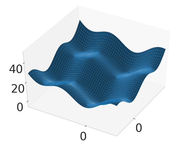
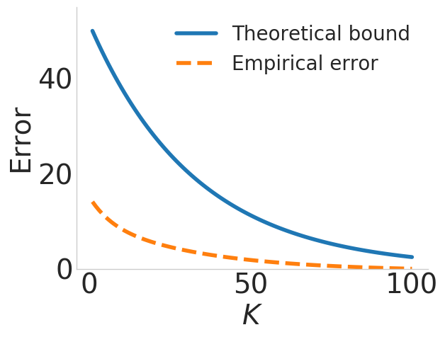
Figure 1: Graph of $f$ and visualization of Prop. 3.1.

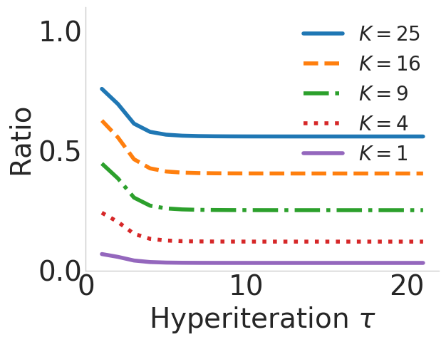
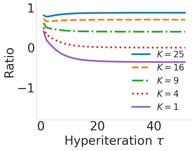
Figure 2: The ratio $h_{T-K}^{\top}\text{d}_{\lambda}f/\|\text{d}_{\lambda}f\|^{2}$ at various $\lambda_{\tau}$, for $f$ and $\widetilde{f}$ respectively.

Figure 1 visualizes Proposition 3.1 by plotting the approximation error $\|h_{T-K}-\text{d}_{\lambda}f\|$ and the theoretical bound $\frac{(1-\gamma\alpha)^{K}}{\gamma\alpha}\|\nabla_{\hat{w}^{*}}f\|M_{B}$ at $\lambda=(1,1)$. For this problem, $\alpha=\frac{1}{2}$, $M_{B}=\|\gamma G\|=\gamma$, and $\nabla_{\hat{w}^{*}}f$ can be found analytically from $\hat{w}^{*}=Cw_{0}+(I-C)\lambda$, where $C=(I-\gamma G)^{T}$. Figure 4 (left) plots the iterates $\lambda_{\tau}$ when optimizing $f$ using $1$-RMD and a decaying meta-learning rate $\eta_{\tau}=\frac{\eta_{0}}{\sqrt{\tau}}$. In comparison with the true gradient $\text{d}_{\lambda}f$ at these points, we see that $h_{T-1}$ is indeed a descent direction. Figure 2 (left) visualizes this in a different way, by plotting $h_{T-K}^{\top}\text{d}_{\lambda}f/\|\text{d}_{\lambda}f\|^{2}$ for various $K$ at each point $\lambda_{\tau}$ along the $K=1$ trajectory. By Lemma 3.2, this ratio stays well away from zero.

To demonstrate the biased convergence of Theorem 3.3, we break assumption 3 of Theorem 3.4 by changing the upper objective to $\widetilde{f}(\hat{w}^{*},\lambda):=f(\hat{w}^{*},\lambda)+5\|\lambda-(1,0)\|^{2}$ so that $\nabla_{\lambda}\widetilde{f}\neq 0$. The guarantee of Lemma 3.2 no longer applies, and we see in Figure 2 (right) that $h_{T-K}^{\top}\text{d}_{\lambda}f/\|\text{d}_{\lambda}f\|^{2}$ can become negative. Indeed, Figure 3 shows that optimizing $\widetilde{f}$ with $h_{T-1}$ converges to a suboptimal point. However, it also shows that using larger $K$ rapidly decreases the bias.

For the original objective $f$, Theorem 3.4 guarantees exact convergence. Figure 4 shows optimization trajectories for various $K$, and a log-scale plot of their convergence rates. Note that, because the lower-level problem cannot be perfectly solved within $T$ steps, the optimal $\lambda$ is offset from the origin. Truncated back-propagation can handle this, but it breaks the assumptions required by the implicit differentiation approach to bilevel optimization.

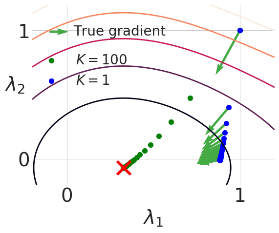
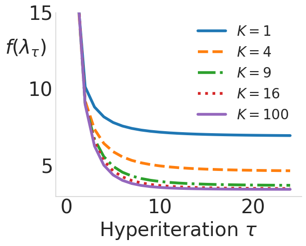
Figure 3: Biased convergence for $\widetilde{f}$. The red X marks the optimal $\lambda$.

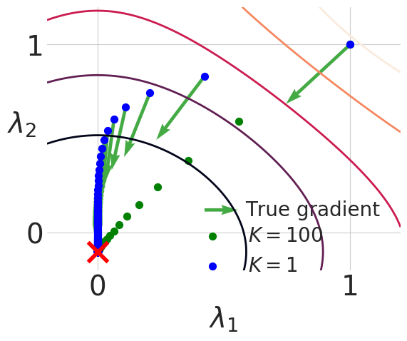
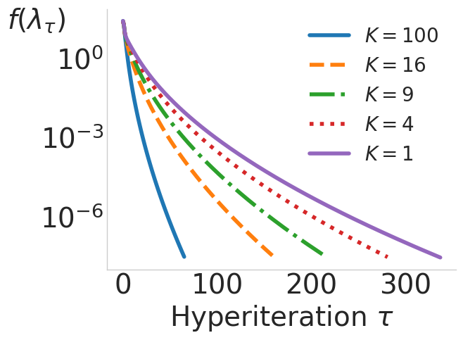
Figure 4: Convergence for $f$.

4.2 Hyperparameter optimization problems

4.2.1 Data hypercleaning

In this section, we evaluate $K$-RMD on a hyperparameter optimization problem. The goal of data hypercleaning [9] is to train a linear classifier for MNIST [30], with the complication that half of our training labels have been corrupted. To do this with hyperparameter optimization, let $W\in\mathbb{R}^{10\times 785}$ be the weights of the classifier, with the outer objective $f$ measuring the cross-entropy loss on a cleanly labeled validation set. The inner objective is defined as weighted cross-entropy training loss plus regularization:

$$\textstyle g(W,\lambda)=\sum_{i=1}^{5000}-\sigma(\lambda_{i})\log(e_{y_{i}}^{\top}Wx_{i})+0.001\|W\|_{F}^{2}$$

where $(x_{i},y_{i})$ are the training examples, $\sigma$ denotes the sigmoid function, $\lambda_{i}\in\mathbb{R}$, and $\|\cdot\|_{F}$ is the Frobenius norm. We optimize $\lambda$ to minimize validation loss, presumably by decreasing the weight of the corrupted examples. The optimization dimensions are $|\lambda|=5000$, $|W|=7850$. Franceschi et al. [9] previously solved this problem with full RMD, and it happens to satisfy many of our theoretical assumptions, making it an interesting case for empirical study.

We optimize the lower-level problem $g$ through $T=100$ steps of gradient descent with $\gamma=1$ and consider how adjusting $K$ changes the performance of $K$-RMD. Our hypothesis is that $K$-RMD for small $K$ works almost as well as full RMD in terms of validation and test accuracy, while requiring less time and far less memory. We also hypothesize that $K$-RMD does almost as well as full RMD in identifying which samples were corrupted [9]. Because our formulation of the problem is unconstrained, the weights $\sigma(\lambda_{i})$ are never exactly zero. However, we can calculate an F1 score by setting a threshold on $\lambda$: if $\sigma(\lambda_{i})<\sigma(-3)\approx 0.047$, then the hyper-cleaner has marked example $i$ as corrupted.

Table 2 reports these metrics for various $K$. We see that $1$-RMD is somewhat worse than the others, and that validation loss (the outer objective $f$) decreases with $K$ more quickly than generalization error. The F1 score is already maximized at $K=5$. These preliminary results indicate that in situations with limited memory, $K$-RMD for small $K$ (e.g. $K=5$) may be a reasonable fallback: it achieves results close to full backprop, and it runs about twice as fast.

Table 2: Hypercleaning metrics after 1000 hyperiters.

$K$	Test Acc.	Val. Acc.	Val. Loss	F1
1	87.50	89.32	0.413	0.85
5	88.05	89.90	0.383	0.89
25	88.12	89.94	0.382	0.89
50	88.17	90.18	0.381	0.89
100	88.33	90.24	0.380	0.88

From a theoretical optimization perspective, we wonder whether $K$-RMD converges to a stationary point of $f$. Data hypercleaning satisfies all of the assumptions of Theorem 3.4 except that $B_{t}$ is not full column rank (since $M<N$). In particular, the validation loss $f$ is deterministic and satisfies $\nabla_{\lambda}f=0$. Figure 5 plots the norm of the true gradient $\text{d}_{\lambda}f$ on a log scale at the $K$-RMD iterates for various $K$. We see that, despite satisfying almost all assumptions, this problem exhibits biased convergence. The limit of $\|\text{d}_{\lambda}f\|$ decreases slowly with $K$, but recall from Table 2 that practical metrics improve more quickly.

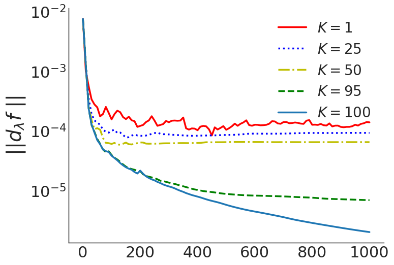
Figure 5: $\|\text{d}_{\lambda}f\|$ vs. hyperiteration for hypercleaning.

4.2.2 Task interaction

We next consider the problem of multitask learning [27]. Similar to [9], we formulate this as a hyperparameter optimization problem as follows. The lower-level objective $g(w,\{C,\rho\})$ learns $V$ different linear models with parameter set $w=\{w_{v}\}_{v=1}^{V}$:

$$l(w)+\sum_{1\leq i,j\leq K}C_{ij}\|w_{i}-w_{j}\|^{2}+\rho\sum_{v=1}^{V}\|w_{v}\|^{2}$$

where $l(w)$ is the training loss of the multi-class linear logistic regression model, $\rho$ is a regularization constant, and $C$ is a nonnegative, symmetric hyperparameter matrix that encodes the similarity between each pair of tasks. After $100$ iterations of gradient descent with learning rate $0.1$, this yields $\hat{w}^{*}$. The upper-level objective $c(\hat{w}^{*})$ estimates the linear regression loss of the learned model $\hat{w}^{*}$ on a validation set. Presumably, this will be improved by tuning $C$ to reflect the true similarities between the tasks. The tasks that we consider are image recognition trained on very small subsets of the datasets CIFAR-$10$ and CIFAR-$100$.

From an optimization standpoint, we are most interested in the upper-level loss on the validation set, since that is what is directly optimized, and its value is a good indication of the performance of the inexact gradient. Figure 6 plots this learning curve along with two other metrics of theoretical interest: norm of the true gradient, and cosine similarity between the true and approximate gradients. In CIFAR100, the validation error and gradient norm plots show that $K$-RMD converges to an approximate stationary point with a bias that rapidly decreases as $K$ increases, agreeing with Proposition 3.1. Also, we find that negative values exist in the cosine similarity of $1$-RMD, which implies that not all the assumptions in Theorem 3.4 hold for this problem (e.g. $B_{t}$ might not be full rank, or the the inner problem might not be locally strong convex around $\hat{w}^{*}$.) In CIFAR10, some unusal behavior happens. For $K>1$, the truncated gradient and the full gradient directions eventually become almost the same. We believe this is a very interesting observation but beyond the scope of the paper to explain.

In Table 3, we report the testing accuracy over 10 trials. While in general increasing the number of back-propagation steps improves accuracy, the gaps are small. A thorough investigation of the relationship between convergence and generalization is an interesting open question of both theoretical and practical importance.

Table 3: Test accuracy for task interaction. Few-step $K$-RMD achieves similar performance as full RMD.

	Method	Avg. Acc.	Avg. Iter.	Sec/iter.
CIFAR-10	$1$-RMD	$61.11\pm 1.23$	$3300$	$0.8$
	$5$-RMD	$61.33\pm 1.08$	$4950$	$1.3$
	$25$-RMD	$61.31\pm 1.24$	$4825$	$1.4$
	Full RMD	$61.28\pm 1.21$	$4500$	$2.2$
CIFAR-100	$1$-RMD	$34.37\pm 0.63$	$7440$	$1.0$
	$5$-RMD	$34.34\pm 0.68$	$8805$	$1.4$
	$25$-RMD	$34.51\pm 0.69$	$8660$	$1.6$
	Full RMD	$34.70\pm 0.64$	$5670$	$2.8$

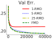
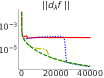
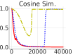
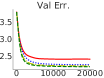
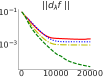
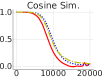
Figure 6: Upper-level objective loss (first column), norm of the exact gradient (second column), and cosine similarity (last column) vs. hyper-iteration on CIFAR10 (first row) and CIFAR100 (second row) datasets.

4.3 Meta-learning: One-shot classification

The aim of this experiment is to evaluate the performance of truncated back-propagation in multi-task, stochastic optimization problems. We consider in particular the one-shot classification problem [20], where each task $\mathcal{T}$ is a $k$-way classification problem and the goal is learn a hyperparameter $\lambda$ such that each task can be solved with few training samples.

In each hyper-iteration, we sample a task, a training set, and a validation set as follows: First, $k$ classes are randomly chosen from a pool of classes to define the sampled task $\mathcal{T}$. Then the training set $S=\{(x_{i},y_{i})\}_{i=1}^{k}$ is created by randomly drawing one training example $(x_{i},y_{i})$ from each of the $k$ classes. The validation set $Q$ is constructed similarly, but with more examples from each class. The lower-level objective $g_{S}(w,\lambda)$ is

$$\textstyle\sum_{(x_{i},y_{i})\in S}l(nn(x_{i};w,\lambda),y_{i})+\sum_{j=1}^{V}\rho_{j}||w_{j}-c_{j}||^{2}$$

where $l(\cdot,\cdot)$ is the $k$-way cross-entropy loss, and $nn(\cdot;w,\lambda)$ is a deep neural network parametrized by $w=\{w_{1},\dots,w_{V}\}$ and optionally hyperparameter $\lambda$. To prevent overfitting in the lower-level optimization, we regularize each parameter $w_{j}$ to be close to center $c_{j}$ with weight $\rho_{j}>0$. Both $c_{j}$ and $\rho_{j}$ are hyperparameters, as well as the inner learning rate $\gamma$. The upper-level objective is the loss of the trained network on the sampled validation set $Q$. In contrast to other experiments, this is a stochastic optimization problem. Also, $\mathcal{A}_{\lambda}(S)(x_{i})=nn(x_{i};\hat{w}^{*},\lambda)$ depends directly on the hyperparameter $\lambda$, in addition to the indirect dependence through $\hat{w}^{*}$ (i.e. $\nabla_{\lambda}f\neq 0$).

We use the Omniglot dataset [31] and a similar neural network as used in [20] with small modifications. Please refer to Appendix G.3 for more details about the model and the data splits. We set $T=50$ and optimize over the hyperparameter $\lambda=\{\lambda_{l_{1}},\lambda_{l_{2}},c,\rho,\gamma\}$. The average accuracy of each model is evaluated over $120$ randomly sampled training and validation sets from the meta-testing dataset. For comparison, we also try using full RMD with a very short horizon $T=1$, which is common in recent work on few-shot learning [20].

The statistics are shown in Table 4 and the learning curves in Figure 7. In addition to saving memory, all truncated methods are faster than full RMD, sometimes even five times faster. These results suggest that running few-step back-propagation with more hyper-iterations can be more efficient than the full RMD. To support this hypothesis, we also ran $1$-RMD and $10$-RMD for an especially large number of hyper-iterations ($15$k). Even with this many hyper-iterations, the total runtime is less than full RMD with $5000$ iterations, and the results are significantly improved. We also find that while using a short horizon ($T=1$) is faster, it achieves a lower accuracy at the same number of iterations.

Finally, we verify some of our theorems in practice. Figure 7 (fourth plot) shows that when the lower-level problem is regularized, the relative $\ell_{2}$ error between the $K$-RMD approximate gradient and the exact gradient decays exponentially as $K$ increases. This was guaranteed by Proposition 3.1. However, this exponential decay is not seen for the non-regularized model ($\rho=0$). This suggests that the local strong convexity assumption is essential in order to have exponential decay in practice. Figure 7 (third plot) shows the cosine similarity between the inexact gradient and full gradient over the course of meta-training. Note that the cosine similarity measures are always positive, indicating that the inexact gradients are indeed descent directions. It also seems that the cosine similarities show a slight decay over time.

Table 4: Results for one-shot learning on Omniglot dataset. $K$-RMD reaches similar performance as full RMD, is considerably faster, and requires less memory.

Method	Accuracy	iter.	Sec/iter.
$1$-RMD	$95.6$	$5$K	$0.4$
$10$-RMD	$96.3$	$5$K	$0.7$
$25$-RMD	$96.1$	$5$K	$1.3$
Full RMD	$95.8$	$5$K	$2.2$
$1$-RMD	$97.7$	$15$K	$0.4$
$10$-RMD	$97.8$	$15$K	$0.7$
Short horizon	$96.6$	$15$K	$0.1$

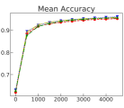
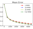
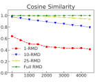
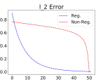
Figure 7: Omniglot results. Plots 1 and 2: Test accuracy and val. error vs. number of hyper-iterations for different RMD depths. $K$-RMD methods show similar performance as the full RMD. Plot 3: Cosine similarity between inexact gradient and full RMD over hyper-iterations. Plot 4: Relative $\ell_{2}$ error of inexact gradient and full RMD vs. reverse depth. Regularized version shows exponential decay.

5 CONCLUSION

We analyze $K$-RMD, a first-order heuristic for solving bilevel optimization problems when the lower-level optimization is itself approximated in an iterative way. We show that $K$-RMD is a valid alternative to full RMD from both theoretical and empirical standpoints. Theoretically, we identify sufficient conditions for which the hyperparameters converge to an approximate or exact stationary point of the upper-level objective. The key observation is that when $\hat{w}^{*}$ is near a strict local minimum of the lower-level objective, gradient approximation error decays exponentially with reverse depth. Empirically, we explore the properties of this optimization method with four proof-of-concept experiments. We find that although exact convergence appears to be uncommon in practice, the performance of $K$-RMD is close to full RMD in terms of application-specific metrics (such as generalization error). It is also roughly twice as fast. These results suggest that in hyperparameter optimization or meta learning applications with memory constraints, truncated back-propagation is a reasonable choice.

Our experiments use a modest number of parameters $M$, hyperparameters $N$, and horizon length $T$. This is because we need to be able to calculate both $K$-RMD and full RMD in order to compare their performance. One promising direction for future research is to use $K$-RMD for bilevel optimization problems that require powerful function approximators at both levels of optimization. Truncated RMD makes this approach feasible and enables comparing bilevel optimization to other meta-learning methods on difficult benchmarks.

Appendix

Appendix A Proof of Proposition 3.1

See 3.1

Proof.

Let $\text{d}_{\lambda}f-h_{T-K}=e_{K}$. By definition of $h_{T-K}$,

$$e_{K}=\left(\sum_{t=0}^{T-K}B_{t}A_{t+1}\cdots A_{T-K}\right)A_{T-K+1}\cdots A_{T}\nabla_{\hat{w}^{*}}f$$

Therefore, when $g$ is locally $\alpha$-strongly convex with respect to $w$ in the neighborhood of $\{w_{T-K-1},\dots,w_{T}\}$,

$$\|e_{K}\| \leq\|\sum_{t=0}^{T-K}B_{t}A_{t+1}\cdots A_{T-K}\|\|A_{T-K+1}\cdots A_{T}\nabla_{\hat{w}^{*}}f\|$$

$$\leq(1-\gamma\alpha)^{K}\|\nabla_{\hat{w}^{*}}f\|\|\sum_{t=0}^{T-K}B_{t}A_{t+1}\cdots A_{T-K}\|$$

Suppose $g$ is $\beta$-smooth but nonconvex. In the worst case, if the smallest eigenvalue of $\nabla_{w,w}g(w_{t-1},\lambda)$ is $-\beta$, then $\|A_{t}\|=1+\gamma\beta\leq 2$ for $t=0,\dots,T-K$. This gives the bound in (9). However, if $g$ is globally strongly convex, then

$$\|e_{K}\| \leq\|\nabla_{\hat{w}^{*}}f\|(1-\gamma\alpha)^{K}\max_{t\in\{0,\dots,T-K\}}\|B_{t}\|\sum_{t=0}^{T-K}(1-\gamma\alpha)^{t}$$

The bound (10) uses the fact that $\sum_{t=0}^{T-K}(1-\gamma\alpha)^{t}\leq\sum_{t=0}^{\infty}(1-\gamma\alpha)^{t}=\frac{1}{\gamma\alpha}$ ∎

Appendix B Proof of Lemma 3.2

See 3.2

Proof.

To illustrate the idea, here we prove the case where $K=1$. For $K>1$, similar steps can be applied. To prove the statement, we first expand the inner product by definition

$$h_{T-1}^{\top}\text{d}_{\lambda}f=\|h_{T-1}\|^{2}+\left(B_{T}\nabla_{\hat{w}^{*}}f\right)^{\top}\left(\sum_{t=0}^{T-1}B_{t}A_{t+1}\cdots A_{T-1}\right)A_{T}\nabla_{\hat{w}^{*}}f$$

where we recall $h_{T-1}=B_{T}\nabla_{\hat{w}^{*}}f$ as $\nabla_{\lambda}f=0$ by assumption.

Next we show a technical lemma, which provides a critical tool to bound the second term above; its proof is given in the next section.

Lemma B.1.

Let $g$ be $\alpha$-strongly convex and $\beta$-smooth. Assume $B_{t}$ and $A_{t}$ are Lipschitz continuous in $w$, and assume $B_{T}$ has full column rank. For $\gamma\leq\frac{1}{\beta}$,

$$\left(B_{T}\nabla_{\hat{w}^{*}}f\right)^{\top}B_{t}A_{t+1}\cdots A_{T}\nabla_{\hat{w}^{*}}f$$

$$\geq(1-\gamma\alpha)^{T-t}\|B_{T}\nabla_{\hat{w}^{*}}f\|^{2}-\|\nabla_{\hat{w}^{*}}f\|^{2}O\left(\frac{e^{-\alpha\gamma(T-1)}}{1-e^{-\alpha\gamma}}+\left(\gamma(\beta-\alpha)\right)^{T-t}\right)$$

By Lemma B.1, we can then write

$$h_{T-1}^{\top}\text{d}_{\lambda}f\geq\|B_{T}\nabla_{\hat{w}^{*}}f\|^{2}\left(1+\sum_{t=0}^{T-1}(1-\gamma\alpha)^{T-t}\right)-\|\nabla_{\hat{w}^{*}}f\|^{2}O\left(\sum_{t=0}^{T-1}\frac{e^{-\alpha\gamma(T-1)}}{1-e^{-\alpha\gamma}}+\left(\gamma(\beta-\alpha)\right)^{T-t}\right)$$

Because

$$\sum_{t=0}^{T-1}\left(\gamma(\beta-\alpha)\right)^{T-t} =\sum_{k=1}^{T}\left(\gamma(\beta-\alpha)\right)^{k}\leq\frac{\gamma(\beta-\alpha)}{1-\gamma(\beta-\alpha)} \because\gamma\leq\beta$$ ()

and $B_{T}^{\top}B_{T}$ is non-singular by assumption,

$$h_{T-1}^{\top}\text{d}_{\lambda}f \geq\|\nabla_{\hat{w}^{*}}f\|^{2}\Omega(1)-\|\nabla_{\hat{w}^{*}}f\|^{2}O\left(\frac{Te^{-\alpha\gamma(T-1)}}{1-e^{-\alpha\gamma}}+\frac{\gamma(\beta-\alpha)}{1-\gamma(\beta-\alpha)}\right)$$

$$\geq C\|\nabla_{\hat{w}^{*}}f\|^{2}$$

for some $c>0$, when $T$ is large enough and $\gamma$ is small enough. The implication holds because $\|\text{d}_{\lambda}f\|\leq O(\|\nabla_{\hat{w}^{*}}f\|)$. ∎

B.1 Proof of Lemma B.1

Proof.

Let $C_{A}$ and $C_{B}$ be the Lipschitz constant of $A_{t}$ and $B_{t}$. First, we see that the inner product can be lower bounded by the following terms

$$\left(B_{T}\nabla_{\hat{w}^{*}}f\right)^{\top}B_{t}A_{t+1}\cdots A_{T}\nabla_{\hat{w}^{*}}f\geq(1-\gamma\alpha)^{T-t}\|B_{T}\nabla_{\hat{w}^{*}}f\|^{2}-\Delta_{1}-\Delta_{2}-\Delta_{3}$$

where

$$\Delta_{1}=C_{B}\|B_{T}\nabla_{\hat{w}^{*}}f\|\|\nabla_{\hat{w}^{*}}f\|\|w_{T-1}-w_{t-1}\|\|A_{t+1}\cdots A_{T}\|$$

$$\Delta_{2}=C_{A}\|B_{T}^{\top}B_{T}\nabla_{\hat{w}^{*}}f\|\|\nabla_{\hat{w}^{*}}f\|\sum_{k=t+1}^{T-1}\|w_{T-1}-w_{k-1}\|\|A_{t+1}\cdots A_{k-1}\|\|A_{T}\|^{T-k}$$

$$\Delta_{3}=\|\nabla_{\hat{w}^{*}}f\|\|B_{T}^{\top}B_{T}\nabla_{\hat{w}^{*}}f\|\|A_{k}-(1-\gamma\alpha)I\|^{T-k}$$

The above lower bounds can be shown by the following inequalities:

$$\left(B_{T}\nabla_{\hat{w}^{*}}f\right)^{\top}B_{t}A_{t+1}\cdots A_{T}\nabla_{\hat{w}^{*}}f$$

$$\geq\nabla_{\hat{w}^{*}}f^{\top}\left(B_{T}^{\top}B_{T}\right)A_{t+1}\cdots A_{T}\nabla_{\hat{w}^{*}}f-C_{B}\|B_{T}\nabla_{\hat{w}^{*}}f\|\|w_{T-1}-w_{t-1}\|\|A_{t+1}\cdots A_{T}\nabla_{\hat{w}^{*}}f\|$$

$$\nabla_{\hat{w}^{*}}f^{\top}\left(B_{T}^{\top}B_{T}\right)A_{t+1}\cdots A_{T}\nabla_{\hat{w}^{*}}f$$

$$\geq\nabla_{\hat{w}^{*}}f^{\top}\left(B_{T}^{\top}B_{T}\right)A_{t+1}\cdots A_{T-2}A^{2}_{T}\nabla_{\hat{w}^{*}}f-C_{A}\|w_{T-1}-w_{T-2}\|\|A_{t+1}\cdots A_{T-2}\|\|A_{T}\|\|B_{T}^{\top}B_{T}\nabla_{\hat{w}^{*}}f\|\|\nabla_{\hat{w}^{*}}f\|$$

$$\geq\nabla_{\hat{w}^{*}}f^{\top}B_{T}^{\top}B_{t}A_{T}^{T-t}\nabla_{\hat{w}^{*}}f-C_{A}\|B_{T}^{\top}B_{T}\nabla_{\hat{w}^{*}}f\|\|\nabla_{\hat{w}^{*}}f\|\sum_{k=t+1}^{T-1}\|w_{T-1}-w_{k-1}\|\|A_{t+1}\cdots A_{k-1}\|\|A_{T}\|^{T-k}$$

$$\nabla_{\hat{w}^{*}}f^{\top}B_{T}^{\top}B_{T}A_{T}^{T-t}\nabla_{\hat{w}^{*}}f\geq(1-\gamma\alpha)^{T-t}\nabla_{\hat{w}^{*}}f^{\top}B_{T}^{\top}B_{T}\nabla_{\hat{w}^{*}}f-\|\nabla_{\hat{w}^{*}}f\|\|B_{T}^{\top}B_{T}\nabla_{\hat{w}^{*}}f\|\|A_{T}-(1-\gamma\alpha)I\|^{T-t}$$

Next we upper bound the error terms: $\Delta_{1}$, $\Delta_{2}$, and $\Delta_{3}$. We will use the fact that gradient descent converges linearly when optimizing a strongly convex and smooth function [25].

Lemma B.2.

Let $w_{0}$ be the initial condition. Running gradient descent to optimize an $\alpha$-strongly convex and $\beta$-smooth function $g$, with step size $0<\gamma\leq\frac{1}{\beta}$, generates a sequence $\{w_{t}\}$ satisfying

$$\|w_{t}-w^{*}\|\leq De^{-\alpha\gamma t}$$ (13)

where $D=\|w_{0}-w^{*}\|$ and $w^{*}=\operatorname*{arg\,min}g(w)$.

Lemma B.2 implies for $T\geq t$, $\|w_{T}-w_{t}\|\leq 2De^{-\alpha\gamma t}$.

Now we proceed to bound the errors $\Delta_{1}$, $\Delta_{2}$, and $\Delta_{3}$.

Bound on $\Delta_{1}$

Because

$$\|w_{T-1}-w_{t-1}\|\|A_{t+1}\cdots A_{T}\| \leq 2De^{-\alpha\gamma(t-1)}(1-\gamma\alpha)^{T-t}$$

$$\leq 2De^{-\alpha\gamma(t-1)}e^{-\gamma\alpha(T-t)}$$

$$=2De^{-\alpha\gamma\left(T-1\right)}$$

we can upper bound $\Delta_{1}$ by

$$\Delta_{1} =C_{B}\|B_{T}\nabla_{\hat{w}^{*}}f\|\|\nabla_{\hat{w}^{*}}f\|\|w_{T-1}-w_{t-1}\|\|A_{t+1}\cdots A_{T}\|$$

$$\leq\|B_{T}\nabla_{\hat{w}^{*}}f\|\|\nabla_{\hat{w}^{*}}f\|\times 2C_{B}De^{-\alpha\gamma\left(T-1\right)}$$

Bound on $\Delta_{2}$

Because

$$\sum_{k=t+1}^{T-1}\|w_{T-1}-w_{k-1}\|\|A_{t+1}\cdots A_{k-1}\|\|A_{T}\|^{T-k} \leq\sum_{k=t+1}^{T-1}2De^{-\alpha\gamma(k-1)}(1-\alpha\gamma)^{k-1-t+T-k}$$

$$\leq 2D(1-\alpha\gamma)^{T-t-1}\sum_{k=t+1}^{T-1}e^{-\alpha\gamma(k-1)}$$

$$\leq 2D(1-\alpha\gamma)^{T-t-1}e^{-\alpha\gamma t}\sum_{k=t+1}^{T-1}e^{-\alpha\gamma(k-t-1)}$$

$$\leq 2De^{-\alpha\gamma(T-1)}\sum_{m=0}^{T-t}e^{-\alpha\gamma m}$$

$$\leq\frac{2D}{1-e^{-\alpha\gamma}}e^{-\alpha\gamma(T-1)}$$

we can upper bound $\Delta_{2}$ by

$$\Delta_{2} =C_{A}\|B_{T}^{\top}B_{T}\nabla_{\hat{w}^{*}}f\|\|\nabla_{\hat{w}^{*}}f\|\sum_{k=t+1}^{T-1}\|w_{T-1}-w_{k-1}\|\|A_{t+1}\cdots A_{k-1}\|\|A_{T}\|^{T-k}$$

$$=\|B_{T}^{\top}B_{T}\nabla_{\hat{w}^{*}}f\|\|\nabla_{\hat{w}^{*}}f\|\times\frac{2C_{A}D}{1-e^{-\alpha\gamma}}e^{-\alpha\gamma(T-1)}$$

Bound on $\Delta_{3}$

Because

$$\|A_{k}-(1-\gamma\alpha)I\|=\|\gamma\left(\alpha I-\nabla_{w}^{2}f(w_{k-1})\right)\|\leq\gamma(\beta-\alpha)$$

we can upper bound $\Delta_{3}$ by

$$\Delta_{3}=\|\nabla_{\hat{w}^{*}}f\|\|B_{T}^{\top}B_{T}\nabla_{\hat{w}^{*}}f\|\|A_{t}-(1-\gamma\alpha)I\|^{T-t} \leq\|\nabla_{\hat{w}^{*}}f\|\|B_{T}^{\top}B_{T}\nabla_{\hat{w}^{*}}f\|\left(\gamma(\beta-\alpha)\right)^{T-t}$$

Final Result

Using the bounds on $\Delta_{1}$, $\Delta_{2}$, and $\Delta_{3}$, we prove the final result.

$$\left(B_{T}\nabla_{\hat{w}^{*}}f\right)^{\top}B_{t}A_{t+1}\cdots A_{T}\nabla_{\hat{w}^{*}}f$$

$$\geq(1-\gamma\alpha)^{T-t}\|B_{T}\nabla_{\hat{w}^{*}}f\|^{2}-\Delta_{1}-\Delta_{2}-\Delta_{3}$$

$$\geq(1-\gamma\alpha)^{T-t}\|B_{T}\nabla_{\hat{w}^{*}}f\|^{2}-\|\nabla_{\hat{w}^{*}}f\|^{2}O\left(\frac{e^{-\alpha\gamma(T-1)}}{1-e^{-\alpha\gamma}}+\left(\gamma(\beta-\alpha)\right)^{T-t}\right)$$

because $B_{T}$ has full column rank and

$$\Delta_{1}+\Delta_{2}+\Delta_{3} \leq\|\nabla_{\hat{w}^{*}}f\|^{2}\left(\frac{2C_{A}D}{1-e^{-\alpha\gamma}}e^{-\alpha\gamma(T-1)}+2C_{B}De^{-\alpha\gamma\left(T-1\right)}+\left(\gamma(\beta-\alpha)\right)^{T-k}\right)$$

$$=\|\nabla_{\hat{w}^{*}}f\|^{2}\times O\left(\frac{e^{-\alpha\gamma(T-1)}}{1-e^{-\alpha\gamma}}+\left(\gamma(\beta-\alpha)\right)^{T-t}\right)\qed$$

Appendix C Proof of Theorem 3.3

See 3.3

Proof.

The proof of this theorem is a standard proof of non-convex optimization with biased gradient estimates. Here we include it for completeness, as part of it will be used later in the proof of Theorem 3.4.

Let $\lambda_{\tau}$ be the $\tau$th iterate. For short hand, we write $\text{d}_{\lambda}f_{(\tau)}=\text{d}_{\lambda}f(\lambda_{\tau})$, and $h_{T-K,(\tau)}=h_{T-K}(\lambda_{\tau})$. Assume $F$ is $L$-smooth and $\|\text{d}_{\lambda}f_{(\tau)}\|\leq G$ and $\|h_{T-K,(\tau)}\|\leq G$ almost surely for all $\tau$. Then by $L$-smoothness, it satisfies

$$F(\lambda_{\tau+1})\leq F(\lambda_{\tau})+\langle\nabla F(\lambda_{\tau}),\lambda_{\tau+1}-\lambda_{\tau}\rangle+\frac{L}{2}\|\lambda_{\tau+1}-\lambda_{\tau}\|^{2}.$$

Let $e_{\tau}=\text{d}_{\lambda}f_{(\tau)}-h_{T-K,(\tau)}$ be the error in the gradient estimate. Substitute the recursive update $\lambda_{\tau+1}=\lambda_{\tau}-\eta_{t}h_{T-K,(\tau)}$ to the above inequality. Conditioned on $\lambda_{\tau}$, it satisfies

$$\mathbb{E}_{|\lambda_{\tau}}[F(\lambda_{\tau+1})]\leq F(\lambda_{\tau})+\mathbb{E}_{|\lambda_{\tau}}\left[-\eta_{t}\langle\nabla F(\lambda_{\tau}),h_{T-K,(\tau)}\rangle+\frac{L\eta_{t}^{2}}{2}\|h_{T-K,(\tau)}\|^{2}\right].$$

Because

$$-\mathbb{E}_{|\lambda_{\tau}}[\langle\nabla F(\lambda_{\tau}),h_{T-K,(\tau)}\rangle] =\mathbb{E}_{|\lambda_{\tau}}\left[-\langle\nabla F(\lambda_{\tau}),\text{d}_{\lambda}f_{(\tau)}\rangle+\langle\nabla F(\lambda_{\tau}),e_{\tau}\rangle\right]$$

$$\leq-\|\nabla F(\lambda_{\tau})\|^{2}+G\|{e_{\tau}}\|$$ (14)

and

$$\frac{1}{2}\|h_{T-K,(\tau)}\|^{2}=\frac{1}{2}\|\text{d}_{\lambda}f_{(\tau)}\|^{2}+\frac{1}{2}\|e_{\tau}\|^{2}-\langle\text{d}_{\lambda}f_{(\tau)},h_{T-K,(\tau)}\rangle\leq\frac{3G^{2}}{2}+\frac{1}{2}\|e_{\tau}\|^{2}$$

we can upper bound $\mathbb{E}_{|\lambda_{\tau}}[F(\lambda_{\tau+1})]$ as

$$\mathbb{E}_{|\lambda_{\tau}}[F(\lambda_{\tau+1})]\leq F(\lambda_{\tau})+\mathbb{E}_{|\lambda_{\tau}}\left[-\eta_{\tau}\|\nabla F(\lambda_{\tau})\|^{2}+\eta_{\tau}G\|{e_{\tau}}\|+L\eta_{\tau}^{2}\left(\frac{3G^{2}}{2}+\frac{1}{2}\|e_{\tau}\|^{2}\right)\right]$$

Performing telescoping sum with the above inequality, we have

$$\mathbb{E}\left[\sum_{\tau=1}^{R}\eta_{\tau}\|\nabla F(\lambda_{\tau})\|^{2}\right] \leq F(\lambda_{1})+\mathbb{E}\left[\sum_{\tau=1}^{R}G\eta_{\tau}\|{e_{\tau}}\|+L\eta_{\tau}^{2}\left(\frac{3G^{2}}{2}+\frac{1}{2}\|e_{\tau}\|^{2}\right)\right]$$

$$\leq F(\lambda_{1})+\sum_{\tau=1}^{R}\left(G\epsilon\eta_{\tau}+\frac{L(3G^{2}+\epsilon^{2})}{2}\eta_{\tau}^{2}\right)$$

Dividing both sides by $\sum_{\tau=1}^{R}\eta_{\tau}$ and using the facts that $\eta_{\tau}=O(\frac{1}{\sqrt{\tau}})$ and that

$$\frac{\sum_{\tau=1}^{R}\frac{1}{\tau}}{\sum_{\tau=1}^{R}\frac{1}{\sqrt{\tau}}}=O\left(\frac{\log R}{\sqrt{R}}\right)$$

proves the theorem. ∎

Appendix D Proof of Theorem 3.4

See 3.4

Proof.

First we consider the special case when $S$ is deterministic. Let $H\geq K$. We decompose the full gradients into four parts

$$\nabla F=\text{d}_{\lambda}f=\nabla_{\lambda}f+q+r+e$$

where

$$q=\sum_{t=T-K+1}^{T}B_{t}A_{t+1}\cdots A_{T}\nabla_{\hat{w}^{*}}f$$

$$r=\sum_{t=T-H+1}^{T-K}B_{t}A_{t+1}\cdots A_{T}\nabla_{\hat{w}^{*}}f$$

$$e=\sum_{t=0}^{T-H}B_{t}A_{t+1}\cdots A_{T}\nabla_{\hat{w}^{*}}f$$

We assume that $w_{t}$ enters a locally strongly convex region for $t\geq H$. This implies, by Proposition 3.1, that $\|e\|\leq O(e^{-\alpha\gamma H}\|\nabla_{\hat{w}^{*}}f\|)$.

To prove the theorem, we first verify two conditions:

1. By Lemma 3.2, the assumption $\nabla_{\lambda}f^{\top}(\text{d}_{\lambda}f+h_{T-K}-\nabla_{\lambda}f)\geq\Omega(\|\nabla_{\lambda}f\|^{2})$, and $\|e\|\leq O(e^{-\alpha\gamma H}\|\nabla_{\hat{w}^{*}}f\|)$:

   $$\text{d}_{\lambda}f^{\top}h_{T-K} =(\nabla_{\lambda}f+q+r+e)^{\top}(\nabla_{\lambda}f+q)$$

   $$=\|\nabla_{\lambda}f\|^{2}+\nabla_{\lambda}f^{\top}(q+e+r)+q^{\top}\nabla_{\lambda}f+q^{\top}(q+r)+q^{\top}e$$

   $$\geq\Omega(\|\nabla_{\lambda}f\|^{2})+q^{\top}(q+r)+q^{\top}e$$ (Assumption)

   $$\geq\Omega(\|\nabla_{\lambda}f\|^{2})+\Omega(\|\nabla_{\hat{w}^{*}}f\|^{2})+q^{\top}e$$ (Lemma 3.2)

   $$\geq\Omega(\|\nabla_{\lambda}f\|^{2})+\Omega(\|\nabla_{\hat{w}^{*}}f\|^{2})-O\left(e^{-\alpha\gamma H}\|\nabla_{\hat{w}^{*}}f\|^{2}\right) \|e\|\leq O(e^{-\alpha\gamma H}\|\nabla_{\hat{w}^{*}}f\|)$$ ()

   where we note

   $$\text{d}_{\lambda}f+h_{T-K}-\nabla_{\lambda}f =\nabla_{\lambda}f+q+r+e+\nabla_{\lambda}f+q-\nabla_{\lambda}f$$

   $$=\nabla_{\lambda}f+q+r+e+q$$

   Therefore, for $H$ large enough, it holds that

   $$\text{d}_{\lambda}f^{\top}h_{T-K}\geq\Omega(\|\nabla_{\lambda}f\|^{2}+\|\nabla_{\hat{w}^{*}}f\|^{2})$$ (15)

2. By definition of $h_{T-K}=\nabla_{\lambda}f+q$, it holds that

   $$\|h_{T-K}\|^{2}\leq 2\|\nabla_{\lambda}f\|^{2}+2\|q\|^{2}\leq O(\|\nabla_{\lambda}f\|^{2}+\|\nabla_{\hat{w}^{*}}f\|^{2})$$ (16)

Next, we prove a lemma

Lemma D.1.

Let $f$ be a lower-bound and $L$-smooth function. Consider the iterative update rule

$$x_{t+1}=x_{t}-\eta g_{t}$$

where $g_{t}$ satisfies $g_{t}^{\top}\nabla f(x_{t})\geq c_{1}h_{t}^{2}$ and $\|g_{t}\|^{2}\leq c_{2}h_{t}^{2}$, for some constant $c_{1},c_{2}>0$ and scalar $h_{t}$. Suppose $f$ is lower-bounded and $\eta$ is chosen such that $\left(-c_{1}\eta+\frac{Lc_{2}\eta^{2}}{2}\right)\leq 0$. Then $\lim\limits_{t\to\infty}h_{t}=0$.

Proof.

By $L$-smoothness,

$$f(x_{t+1})-f(x_{t}) \leq\nabla f(x_{t})^{\top}(x_{t+1}-x_{t})+\frac{L}{2}\|x_{t+1}-x_{t}\|^{2}$$

$$=-\eta\nabla f(x_{t})^{\top}g_{t}+\frac{L\eta^{2}}{2}\|g_{t}\|^{2}$$

$$\leq\left(-c_{1}\eta+\frac{Lc_{2}\eta^{2}}{2}\right)h_{t}^{2}$$

By telescoping sum, we can show $\sum_{t=0}^{\infty}\left(c\eta-\frac{L\eta^{2}}{2}\right)h_{t}^{2}<\infty$, which implies $\lim_{t\to\infty}h_{t}=0$. ∎

Finally, we prove the main theorem by applying Lemma D.1. Consider a deterministic problem. Take $h_{t}^{2}=\|\nabla_{\lambda}f(\lambda_{t})\|^{2}+\|\nabla_{\hat{w}^{*}}f(\lambda_{t})\|^{2}$. Because of (15) and (16), by Lemma D.1, it satisfies that

$$\lim_{t\to\infty}h_{t}=\lim_{t\to\infty}\|\nabla_{\lambda}f(\lambda_{t})\|^{2}+\|\nabla_{\hat{w}^{*}}f(\lambda_{t})\|^{2}=0$$

As $\|\text{d}_{\lambda}f\|\leq O(\|\nabla_{\lambda}f\|+\|\nabla_{\hat{w}^{*}}f\|)$, it shows $\|\text{d}_{\lambda}f\|$ converges to zero in the limit.

∎

Appendix E Proof of Theorem 3.5

See 3.5

Proof.

We prove the non-convergence using the following strategy. First we show that, when assumption 3 in Theorem 3.4, i.e.

$$\nabla_{\lambda}f^{\top}(\text{d}_{\lambda}f+h_{T-K}-\nabla_{\lambda}f)\geq\Omega(\|\nabla_{\lambda}f\|^{2})$$ (17)

does not hold, there is some problem such that $h_{T-k}\neq 0$ for all stationary points (i.e. $\lambda$ such that $\text{d}_{\lambda}f=0$). Then we show that, for such a problem, optimizing $\lambda$ with $h_{T-k}$ cannot converge to any of the stationary points.

Counter example

To construct the counterexample, we consider a scalar deterministic bilevel optimization problem of the form

$$\begin{split}&\min_{\lambda}\frac{1}{2}(\hat{w}^{*})^{2}+\phi(\lambda)\\ \text{s.t.}\quad&\hat{w}^{*}\approx w^{*}\in\operatorname*{arg\,min}_{w}\frac{1}{2}(w-\lambda)^{2}\end{split}$$ (18)

in which $\phi$ is some perturbation function that we will later define, and $\hat{w}^{*}$ is computed by performing $T>1$ steps of gradient descent in the lower-level optimization problem with some constant initial condition $w_{0}$ and constant step size $0<\gamma<1$, i.e.

$$\hat{w}^{*}=w_{T},\qquad w_{t+1}=w_{t}-\gamma(w_{t}-\lambda)$$

We can observe this problem satisfies almost all the assumptions in Theorem 3.4:

1. The lower-level objective $g$ is smooth and strongly convex. (Proposition 3.1)

2. The upper-level objective $F$ is smooth. (Theorem 3.3)

3. The lower-level objective $g$ is second-order continuously differentiable (assumption 1 in Theorem 3.4)

4. The Jacobian if full rank, i.e. $B_{t}=\gamma>0$ (assumption 2 in Theorem 3.4)

5. The upper-level objective function is deterministic, i.e. $F=f$ (assumption 4 in Theorem 3.4)

But we will show that properly setting $\phi$ can break the non-interfering assumption in (17) (i.e. assumption 3 in Theorem 3.4) and then creates a problem such that optimizing $\lambda$ with $K$-RMD does not converge to an exact stationary point.

We follow the two-step strategy mentioned above.

Step 1: Non-vanishing approximate gradient

Without loss of generality, let us consider optimizing $\lambda$ with $1$-RMD. In this case we can write the approximate and the exact gradients in closed form as

$$h_{T-1}=\nabla\phi+w^{*}\gamma,\qquad\text{d}_{\lambda}f=\nabla\phi+w^{*}\gamma\sum_{t=0}^{T}(1-\gamma)^{T-t}$$ (19)

which are given by (5) and (8). We will show that by properly choosing $\phi$, we can define $f(\lambda)=\frac{1}{2}(\hat{w}^{*})^{2}+\phi(\lambda)$ such that, at any of the stationary points of $f$, the approximate gradient of $1$-RMD does not vanish. That is, we show when $\text{d}_{\lambda}f=0$, $h_{T-1}\neq 0$.

Before proceeding, let us define $u=w^{*}\gamma$ and $v=w^{*}\gamma\sum_{t=0}^{T}(1-\gamma)^{T-t}$ for convenience. To show how to construct $\phi$, let us consider the stationary points in the case when $\phi=0$. Let $P_{0}$ denote the set of these stationary points, i.e. $P_{0}=\{\lambda:v=0\}$. Since $f$ is smooth and lower-bounded, we know that $P_{0}$ is non-empty, and from the construction of our counterexample we know that $P_{0}$ contains exactly the $\lambda$s such that $w^{*}=0$.

This implies that for $\lambda\in\mathbb{R}\backslash P_{0}$, it satisfies $w^{*}\neq 0$ and therefore

$$uv=(w^{*}\gamma)^{2}\sum_{t=0}^{T}(1-\gamma)^{T-t}>0$$ (20)

We use this fact to pick an adversarial $\phi$. Consider any smooth, lower-bounded $\phi$ whose stationary points are not in $P_{0}$, e.g. $\phi(\lambda)=\frac{1}{2}(\lambda-\lambda_{0})^{2}$ and $\lambda_{0}\notin P_{0}$. Then $f(\lambda)=\frac{1}{2}(\hat{w}^{*})^{2}+\phi(\lambda)$ has a non-empty set of stationary points $P_{\phi}$ such that $P_{\phi}\cap P_{0}=\emptyset$. We see that, for such $\phi$, the non-interfering assumption (assumption 3 in Theorem 3.4) is violated in $P_{\phi}$:

$$\nabla_{\lambda}f^{\top}(\text{d}_{\lambda}f+h_{T-1}-\nabla_{\lambda}f) =\nabla_{\lambda}f^{\top}(\nabla_{\lambda}f+u-\nabla_{\lambda}f) \because\text{d}_{\lambda}f=0 h_{T-1}=\nabla_{\lambda}f+u$$ and

$$=\nabla_{\lambda}\phi^{\top}u$$

$$=-vu \because 0=\text{d}_{\lambda}f=\nabla_{\lambda}\phi+v$$

$$<0 \because\eqref{eq:uv inequality} P_{\phi}\cap P_{0}=\emptyset$$ and

$$<(\nabla_{\lambda}\phi)^{2} \because v>0 \lambda\in P_{\phi}$$ for

And we show for any $\lambda\in P_{\phi}$ it holds that $h_{T-1}\neq 0$. This can be seen from the definition

$$h_{T-1}=\nabla\phi+u=\text{d}_{\lambda}f+u-v=u-v\neq 0$$

where the last inequality is because $w^{*}\neq 0$ for $\lambda\in P_{\phi}$.

Step 2: Non-convergence to any stationary point

We have shown that there is a problem which satisfies all the assumptions but assumption 3 of Theorem 3.4, and at any of its stationary points (i.e. when $\text{d}_{\lambda}f=0$) we have $h_{T-K}\neq 0$. Now we show this property implies failure to converge to the stationary points for the general problems considered in Theorem 3.5 (i.e. we do not rely on the form made in Step 1 anymore).

We prove this by contradiction. Let $\lambda^{*}$ be one of the stationary points. We choose $\delta_{0}>0$ such that, for some $\epsilon>0$, $\|h_{T-K}\|>\epsilon/\gamma$ for all $\lambda$ inside the neighborhood $\{\lambda:\|\lambda-\lambda^{*}\|<\frac{\delta_{0}}{2}\}$, where we recall $\gamma$ is the step size of the lower-level optimization problem. A non-zero $\delta_{0}$ exists because $h_{T-1}$ is continuous by our assumption and $h_{T-K}\neq 0$ at $\lambda^{*}$.

We are ready to show the contradiction. Let $\delta=\min\{\delta_{0},\epsilon\}$. Suppose there is a sequence $\{\lambda_{\tau}\}$ that converges to the stationary point $\lambda^{*}$. This means that there is $0<M<\infty$ such that, $\forall\tau\geq M$, $\|\lambda_{\tau}-\lambda^{*}\|<\frac{\delta}{2}$, which implies that $\forall\tau\geq M$, $\|\lambda_{\tau+1}-\lambda_{\tau}\|<\delta$. However, by our choice of $\delta_{0}$, $\|\lambda_{\tau+1}-\lambda_{\tau}\|=\gamma\|h_{T-K}\|>\epsilon\geq\delta$, leading to a contradiction.

Thus, no sequence $\{\lambda_{\tau}\}$ converges to any of the stationary points. This concludes our proof. ∎

Appendix F Proof of Proposition 3.6

See 3.6

Proof.

Recall our shorthand that $\nabla_{\lambda,w}g$ and $\nabla_{w,w}g$ are evaluated at $(w^{*},\lambda)$. In the limit, it holds that

$$\lim_{t}A_{t} =\lim_{t}\nabla_{w}\Xi_{t}(w_{t-1},\lambda)=\nabla_{w}(w^{*}-\gamma\nabla_{w}g(w^{*},\lambda))=I-\gamma\nabla_{w,w}g\eqqcolon A_{\infty}$$

$$\lim_{t}B_{t} =\lim_{t}\nabla_{\lambda}\Xi_{t}(w_{t-1},\lambda)=\nabla_{\lambda}(w^{*}-\gamma\nabla_{w}g(w^{*},\lambda))=-\gamma\nabla_{\lambda,w}g\eqqcolon B_{\infty}$$

To prove the equality (12), we use Lemma (F.1).

Lemma F.1.

[32] For a matrix $A$ with $\|A\|<1$, it satisfies that

$$(I-A)^{-1}=\sum_{k=0}^{\infty}A^{k}$$

Since $\gamma\leq\frac{1}{\beta}$, we have $\gamma\alpha I\preceq\gamma\nabla_{w,w}g\preceq I$, so $\|I-\gamma\nabla_{w,w}g\|<1$. By Lemma F.1,

$$\nabla_{w,w}^{-1}g=\gamma(I-I+\gamma\nabla_{w,w}g)^{-1}=\gamma\sum_{k=0}^{\infty}(I-\gamma\nabla_{w,w}g)^{k}=\gamma\sum_{k=0}^{\infty}A_{\infty}^{k}$$

Therefore,

$$-\nabla_{\lambda,w}g\nabla_{w,w}^{-1}g=\left(-\gamma\nabla_{\lambda,w}g\right)\left(\frac{1}{\gamma}\nabla_{w,w}^{-1}g\right)=B_{\infty}\sum_{k=0}^{\infty}A_{\infty}^{k}$$

∎

Appendix G Detailed experimental setup

In this appendix, we provide more details about the settings we used in each experiment. We use Adam [33] to optimize the upper-level objective and vanilla gradient descent for the lower objective. We denote by $\hat{w}^{*}$ the results of running $T$ steps of gradient descent with step size $\gamma$.

G.1 Data hypercleaning

In this appendix, we provide more details about the data hypercleaning experiment on MNIST from Section 4.2.1.

Both the training and the validation sets consist of 5000 class-balanced examples from the MNIST dataset. The test set consists of the remaining examples. For each training example, with probability $\frac{1}{2}$, we replaced the label with a uniformly random one.

For various $K$, we performed $K$-RMD for 1000 hyperiterations. Like in the toy experiment (Section 4.1) we adjusted the initial meta-learning rate $\eta_{0}$ for each $K$ so that the norm of the initial update was roughly the same for each $K$.

We asserted earlier that the reported F1 scores are not sensitive to our choice of threshold $\lambda_{i}<-3$. To validate this assertion, we repeated the experiment for various thresholds. F1 scores are reported in the table below.

$K$	$\lambda_{i}<-4$	$\lambda_{i}<-3$	$\lambda_{i}<-1$
1	0.84	0.84	0.84
5	0.89	0.89	0.90
25	0.89	0.89	0.89
50	0.89	0.89	0.89
100	0.89	0.89	0.89

We only ran these experiments for $150$ hyperiterations, because the F1 score has essentially converged by that point. Indeed, the plot below shows identification of corrupted labels for $K=1$, with cutoff $\lambda_{i}<-4$. The X axis is in units of 1000 hyperiterations. We see that $1$-RMD rapidly identifies most of the mislabeled examples, with a few false positives.

G.2 Task interaction

We use $T=100$ iterations of gradient descent with learning rate $0.1$ in the lower objective which yields $\hat{w}_{S}^{*}$. To ensure that $C$ is symmetric, and that $C_{ij}$ and $\rho$ are nonnegative, we re-parametrize them as $\rho=\text{softplus}(\nu)$ and $C=A+A^{\top}$, where $A_{ij}=\text{softplus}(B_{ij})$ and $B$ is a hyperparameter matrix. Thus, the hyperparameters to be optimized are $\lambda=\{B,\nu\}$.

Rather than using raw pixels, we extract image features from the output of the average pooling layer in Resnet-$18$ [34] which is trained on ImageNet [35]. We use the same data pre-processing that is used for training Resnet architecture.

When reporting test accuracy, we run 10 independent trials. In each trial, we sample the training and validation datasets with a balanced set of $m$ examples each ($m=50$ for CIFAR-10 and $m=300$ for CIFAR-100) and use the rest of the dataset for testing. To avoid over-fitting, we use early stopping when the testing error does not improve for $500$ hyper-iterations.

Although we are using a similar setting as Franceschi et al. [9], our results on full back-propagation are quite different from theirs. We believe it is because we are using a different network architecture and pre-processing method for feature extraction.

G.3 One-shot classification

Dataset

The Omniglot dataset [31], a popular benchmark for few-shot learning, is used in this experiment. We consider $5$-way classification with $1$ training and $15$ validation examples for each of the five classes. To evaluate the generalization performance, we restrict the meta-training dataset to a random subset of $1200$ of the $1623$ Omniglot characters. The meta-validation dataset consists of $100$ other characters, and meta-testing dataset has the remaining $323$ characters. We use the meta-validation dataset for tuning the upper-level optimization parameters and report the performance of the algorithm on the meta-testing dataset. Note that no data augmentation method is used in the training.

Neural Network and Optimization

The overall neural network architecture is shown in Figure 8. Our architecture inherits the hyper-representation model of Franceschi et al. [2] with some modifications. The first two convolutional layers, parametrized by hyperparameter $\lambda=\{\lambda_{l_{1}},\lambda_{l_{2}}\}$, transform the input image into a “hyper-representation” space. The last three layers, parametrized by $w=\{w_{l_{3}},w_{l_{4}},w_{l_{5}}\}$ are fine-tuned in the lower-level optimization. Additionally, we have regularization hyperparameters $\lambda_{r}=\{\rho_{i}\}_{i=1}^{3}\cup\{c_{j}\}_{j=1}^{3}$. The overall setup corresponds essentially to meta-learning the two bottom layers of a CNN; for each task, the weights in the first two layers are frozen, and the $k$-way classifier of the last three layers is fine tuned. Overall, the model has $\approx 110$k hyperparameters and $\approx 75$k parameters.

We use a meta-batch-size of $4$ in each hyper-iteration. To limit the training time, we stop all the algorithms after $5000$ hyper-iterations. Needless to say, these results could be further improved by using data augmentation, higher meta-batch size, and running more hyper-iterations. However, our current setup is selected so that all the experiments can be run in a reasonable amount of time, while sharing a similar setting used in practical one-shot learning.

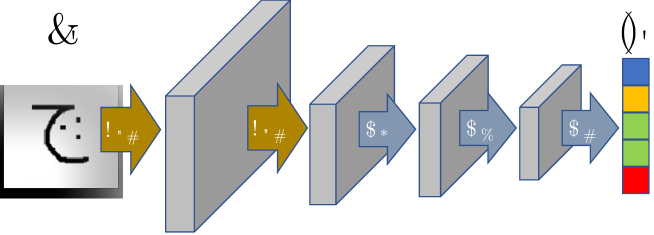
Figure 8: One-shot learning network architecture. The first two convolutional layers map the input image into a ”hyper-representation” space which is frozen while optimizing the lower-level objective. The last three layers are tuned for each task and regularized to avoid overfitting. All the convolutional layers have $64$ $3\times 3$ kernels. There is a max-pooling layer followed by a batch-normalization and a ReLU layer after each convolution.

References

- Domke [2012] Justin Domke. Generic methods for optimization-based modeling. In Artificial Intelligence and Statistics, pages 318–326, 2012.
- Franceschi et al. [2017a] Luca Franceschi, Michele Donini, Paolo Frasconi, and Massimiliano Pontil. A bridge between hyperparameter optimization and larning-to-learn. NIPS 2017 Workshop on Meta-learning, 2017a.
- Bergstra and Bengio [2012] James Bergstra and Yoshua Bengio. Random search for hyper-parameter optimization. Journal of Machine Learning Research, 13(Feb):281–305, 2012.
- Srinivas et al. [2010] Niranjan Srinivas, Andreas Krause, Sham M Kakade, and Matthias Seeger. Gaussian process optimization in the bandit setting: No regret and experimental design. In Proceedings of the 27th International Conference on International Conference on Machine Learning, 2010.
- Snoek et al. [2012] Jasper Snoek, Hugo Larochelle, and Ryan P Adams. Practical bayesian optimization of machine learning algorithms. In Advances in neural information processing systems, pages 2951–2959, 2012.
- Pedregosa [2016] Fabian Pedregosa. Hyperparameter optimization with approximate gradient. In International Conference on Machine Learning, pages 737–746, 2016.
- Gould et al. [2016] Stephen Gould, Basura Fernando, Anoop Cherian, Peter Anderson, Rodrigo Santa Cruz, and Edison Guo. On differentiating parameterized argmin and argmax problems with application to bi-level optimization. arXiv preprint arXiv:1607.05447, 2016.
- Maclaurin et al. [2015] Dougal Maclaurin, David Duvenaud, and Ryan Adams. Gradient-based hyperparameter optimization through reversible learning. In International Conference on Machine Learning, pages 2113–2122, 2015.
- Franceschi et al. [2017b] Luca Franceschi, Michele Donini, Paolo Frasconi, and Massimiliano Pontil. Forward and reverse gradient-based hyperparameter optimization. In Proceedings of the 34th International Conference on International Conference on Machine Learning, 2017b.
- Luketina et al. [2016] Jelena Luketina, Mathias Berglund, Klaus Greff, and Tapani Raiko. Scalable gradient-based tuning of continuous regularization hyperparameters. In International Conference on Machine Learning, pages 2952–2960, 2016.
- Baydin et al. [2018] Atilim Gunes Baydin, Robert Cornish, David Martinez Rubio, Mark Schmidt, and Frank Wood. Online learning rate adaptation with hypergradient descent. In International Conference on Learning Representations, 2018.
- Larsen et al. [1996] Jan Larsen, Lars Kai Hansen, Claus Svarer, and M Ohlsson. Design and regularization of neural networks: the optimal use of a validation set. In Neural Networks for Signal Processing [1996] VI. IEEE Signal Processing Society Workshop, pages 62–71. IEEE, 1996.
- Bengio [2000] Yoshua Bengio. Gradient-based optimization of hyperparameters. Neural computation, 12(8):1889–1900, 2000.
- Chen et al. [2014] Yunjin Chen, Rene Ranftl, and Thomas Pock. Insights into analysis operator learning: From patch-based sparse models to higher order mrfs. IEEE Transactions on Image Processing, 23(3):1060–1072, 2014.
- Caruana [1998] Rich Caruana. Multitask learning. In Learning to learn, pages 95–133. Springer, 1998.
- Ranjan et al. [2017] Rajeev Ranjan, Vishal M Patel, and Rama Chellappa. Hyperface: A deep multi-task learning framework for face detection, landmark localization, pose estimation, and gender recognition. IEEE Transactions on Pattern Analysis and Machine Intelligence, 2017.
- Fei-Fei et al. [2006] Li Fei-Fei, Rob Fergus, and Pietro Perona. One-shot learning of object categories. IEEE transactions on pattern analysis and machine intelligence, 28(4):594–611, 2006.
- Ravi and Larochelle [2017] Sachin Ravi and Hugo Larochelle. Optimization as a model for few-shot learning. In International Conference on Learning Representations, 2017.
- Snell et al. [2017] Jake Snell, Kevin Swersky, and Richard S Zemel. Prototypical networks for few-shot learning. In Advances in Neural Information Processing Systems, 2017.
- Finn et al. [2017] Chelsea Finn, Pieter Abbeel, and Sergey Levine. Model-agnostic meta-learning for fast adaptation of deep networks. In International Conference on Machine Learning (ICML), 2017.
- Andrychowicz et al. [2016] Marcin Andrychowicz, Misha Denil, Sergio Gomez, Matthew W Hoffman, David Pfau, Tom Schaul, and Nando de Freitas. Learning to learn by gradient descent by gradient descent. In Advances in Neural Information Processing Systems, pages 3981–3989, 2016.
- Li and Malik [2017] Ke Li and Jitendra Malik. Learning to optimize neural nets. arXiv preprint arXiv:1703.00441, 2017.
- Baydin et al. [2017] Atilim Gunes Baydin, Barak A Pearlmutter, Alexey Andreyevich Radul, and Jeffrey Mark Siskind. Automatic differentiation in machine learning: A survey. Journal of Machine Learning Research, 18:153:1–153:43, 2017.
- Hascoet and Araya-Polo [2006] Laurent Hascoet and Mauricio Araya-Polo. Enabling user-driven checkpointing strategies in reverse-mode automatic differentiation. arXiv preprint cs/0606042, 2006.
- Hazan et al. [2016] Elad Hazan et al. Introduction to online convex optimization. Foundations and Trends® in Optimization, 2(3-4):157–325, 2016.
- Roth and Black [2005] Stefan Roth and Michael J Black. Fields of experts: A framework for learning image priors. In IEEE Conference on Computer Vision and Pattern Recognition (CVPR), volume 2, pages 860–867. IEEE, 2005.
- Evgeniou et al. [2005] Theodoros Evgeniou, Charles A Micchelli, and Massimiliano Pontil. Learning multiple tasks with kernel methods. Journal of Machine Learning Research, 6(Apr):615–637, 2005.
- Rudin [1964] Walter Rudin. Principles of Mathematical Analysis, volume 3. New York: McGraw-Hill, 1964.
- Shewchuk [1994] Jonathan Richard Shewchuk. An introduction to the conjugate gradient method without the agonizing pain, 1994.
- LeCun et al. [1998] Yann LeCun, Léon Bottou, Yoshua Bengio, and Patrick Haffner. Gradient-based learning applied to document recognition. Proceedings of the IEEE, 86(11):2278–2324, 1998.
- Lake et al. [2015] Brenden M Lake, Ruslan Salakhutdinov, and Joshua B Tenenbaum. Human-level concept learning through probabilistic program induction. Science, 350(6266):1332–1338, 2015.
- Horn and Johnson [1990] Roger A Horn and Charles R Johnson. Matrix analysis. Cambridge University Press, 1990.
- Kingma and Ba [2015] Diederik P Kingma and Jimmy Ba. Adam: A method for stochastic optimization. In International Conference on Learning Representations, 2015.
- He et al. [2016] Kaiming He, Xiangyu Zhang, Shaoqing Ren, and Jian Sun. Deep residual learning for image recognition. In IEEE Conference on Computer Vision and Pattern Recognition (CVPR), pages 770–778, 2016.
- Deng et al. [2009] Jia Deng, Wei Dong, Richard Socher, Li-Jia Li, Kai Li, and Li Fei-Fei. Imagenet: A large-scale hierarchical image database. In IEEE Conference on Computer Vision and Pattern Recognition (CVPR), pages 248–255. IEEE, 2009.