Loop corrections in spin models through density consistency

Abstract

Computing marginal distributions of discrete or semi-discrete Markov Random Fields (MRF) is a fundamental, generally intractable, problem with a vast number of applications on virtually all fields of science. We present a new family of computational schemes to calculate approximately marginals of discrete MRFs. This method shares some desirable properties with Belief Propagation, in particular providing exact marginals on acyclic graphs; but at difference with it, it includes some loop corrections, i.e. it takes into account correlations coming from all cycles in the factor graph. It is also similar to Adaptive TAP, but at difference with it, the consistency is not on the first two moments of the distribution but rather on the value of its density on a subset of values. Results on random connectivity and finite dimensional Ising and Edward-Anderson models show a significant improvement with respect to the Bethe-Peierls (tree) approximation in all cases, and with respect to Plaquette Cluster Variational Method approximation in many cases. In particular, for the critical inverse temperature $\beta_{c}$ of the homogeneous hypercubic lattice, the expansion of $\left(d\beta_{c}\right)^{-1}$ around $d=\infty$ of the proposed scheme is exact up to the $d^{-4}$ order, whereas the two latter are exact only up to the $d^{-2}$ order.

Introduction.

Markov random fields (MRF) are undirected probabilistic graphical models in which random variables satisfy a conditional independence property, so that the joint probability measure can be expressed in a factorized form, each factor involving a possibly different subset of variables (Lauritzen, 1996). Computing marginal distributions of discrete or semi-discrete Markov Random Fields is a fundamental step in most approximate inference methods and high-dimensional estimation problems (MacKay, 2003), such as the evaluation of equilibrium observables in statistical mechanics models. The exact calculation of marginal distributions is however intractable in general, and it is common to resort to stochastic sampling algorithms, such as Monte-Carlo Markov Chain, to obtain unbiased estimates of the relevant quantities. On the other hand, it is also useful to derive approximations of the true probability distribution, for which marginal quantities can be deterministically computed. An important family of approximations is the one of mean-field (MF) schemes. The simplest is naive mean-field (nMF), that neglects all correlations between random variables. An improved MF approximation (Opper et al., 2001), called Thouless-Anderson-Palmer (TAP) equations, works well for models with weak dependencies but it is usually unsuitable for MRFs on diluted models. Here, a considerable improvement is provided by the Bethe-Peierls approximation or Belief Propagation (BP), that is exact for probabilistic models defined on graphs without loops (Mezard and Montanari, 2009). It is a matter of fact that BP has been successfully employed even in on loopy probabilistic models both in physics and in applications (see e.g. Berrou et al. (1993)), yet the lack of analytical control on the effect of loops calls for novel approaches that could systematically improve with respect to BP. A traditional way to account for the effect of short loops is by means of Cluster Variational Methods (CVM), that treat exactly correlations generated between variables within a finite region $\mathcal{R}$ (Kikuchi, 1951; Yedidia et al., 2003; Pelizzola, 2005). The main limitation of CVM resides in its algorithmic complexity, that grows exponentially with the size of the region $\mathcal{R}$. A completely different path to systematically improve BP is represented by loop series expansions (Chertkov and Chernyak, 2006; Gómez et al., 2007; Parisi and Slanina, 2006; Altieri et al., 2017) in which BP is obtained as a saddle-point in a corresponding effective field theory. Loop corrections to BP equations can be alternatively introduced in terms of local equations for correlation functions, as first suggested for pairwise models (Montanari and Rizzo, 2005) and later extended to arbitrary factor graphs (Mooij et al., 2007; Rizzo et al., 2007; Ohzeki, 2013). This method consists in considering deformed local marginal probabilities on a “cavity graph”, obtained removing a factor node (i.e. interaction), and imposing a consistency condition on single-node marginals. On trees, BP equations are recovered, whereas on loopy graphs the obtained set of equations is strongly under-determined and requires additional constraints. Linear-response relations were exploited to this purpose in (Montanari and Rizzo, 2005), even though other moment closure methods are possible (Mooij et al., 2007).

A different approach to approximate inference exploits the properties of multivariate Gaussian distributions, that have the advantage of retaining information on correlations albeit allowing for explicit calculations. In particular, Expectation Propagation (EP, which can be thought as an adaptive variant of TAP) is a very successful algorithmic technique in which a tractable approximate distribution is obtained as the outcome of an iterative process in which the parameters of a multivariate Gaussian are optimized by means of local moment matching conditions (Minka, 2001; Opper and Winther, 2001). EP has been applied to problems involving discrete random variables by employing atomic measures (Opper and Winther, 2005). In the present work, we put forward a new family of computational schemes to calculate approximate marginals of discrete MRFs. We exploits the flexibility of multivariate Gaussian approximation methods but, unlike EP and inspired by beliefs marginalization condition in BP, we impose that marginals on discrete variables are locally consistent, a condition that we call density consistency. When the underlying graph is a tree, the set of equations produced is equivalent to BP. As for Ref.(Montanari and Rizzo, 2005), the density consistency condition leaves an under-determined system of equations on loopy graphs, that can be solved once supplemented with a further set of closure conditions. As a result of employing Gaussian distributions, higher order correlation functions between neighbors of a given variable are, at least partially, taken into account.

The Model.

Consider a factorized distribution of binary variables $x_{1},\dots,x_{n}\in X=\left\{-1,1\right\}$ for arbitrary positive factors $\psi_{a}:X_{a}\to\mathbb{R}_{+}$, each depending on a sub-vector $\boldsymbol{x}_{a}=\left\{x_{i}\right\}_{i\in\partial a}\in X_{a}$

$$p\left(\boldsymbol{x}\right)=\frac{1}{z}\prod_{a\in A}\psi_{a}\left(\boldsymbol{x}_{a}\right).$$ (1)

The bipartite graph $G=\left(V,E\right)$ with $V=I\cup A$ the disjoint union of variable indices $I=\left\{1,\dots,n\right\}$ and factor indices and $E=\left\{\left(ia\right):i\in\partial a\right\}$, is called the factor graph of the factorization (1), and as we will see some of its topological features are crucial to devise good approximations. Particular important cases of (1) include e.g. Ising spin models, many neural network models and the uniform distribution of solutions of $k-$SAT formulas. Computing marginal distributions from (1) is in general NP-Hard (i.e. computationally intractable).

Density Consistency.

Following Gaussian Expectation Propagation (otherwise called adaptive TAP or Expectation Consistency) (Opper and Winther, 2001; Minka, 2001), we will approximate an intractable $p\left(\boldsymbol{x}\right)$ by a Normal distribution $g\left(\boldsymbol{x}\right)$. To do so, we will replace each $\psi_{a}\left(\boldsymbol{x}_{a}\right)$ by an appropriately defined multivariate normal distribution $\phi_{a}\left(\boldsymbol{x}_{a}\right)=\mathcal{N}\left(\boldsymbol{x}_{a};\boldsymbol{\mu}^{a},\boldsymbol{\Sigma}^{a}\right)$. Parameters $\boldsymbol{\mu}^{a},\boldsymbol{\Sigma}^{a}$ will be selected as follows. First define

$$g\left(\boldsymbol{x}\right)=\frac{1}{z_{g}}\prod_{a}\phi_{a}\left(\boldsymbol{x}_{a}\right)=\frac{1}{z^{\prime}}e^{-\frac{1}{2}\left(\boldsymbol{x}-\boldsymbol{\mu}\right)^{T}\boldsymbol{\Sigma}^{-1}\left(\boldsymbol{x}-\boldsymbol{\mu}\right)}.$$

and $g^{\left(a\right)}\left(\boldsymbol{x}\right)=\frac{1}{z_{a}}g\left(\boldsymbol{x}\right)\sum_{\hat{\boldsymbol{x}}_{a}\in X_{a}}\delta\left(\boldsymbol{x}_{a}-\hat{\boldsymbol{x}}_{a}\right)\frac{\psi_{a}\left(\hat{\boldsymbol{x}}_{a}\right)}{\phi_{a}\left(\hat{\boldsymbol{x}}_{a}\right)}$, $g^{\left(i\right)}\left(\boldsymbol{x}\right)=\frac{1}{z_{i}}g\left(\boldsymbol{x}\right)\sum_{\hat{x}_{i}\in X}\delta\left(x_{i}-\hat{x}_{i}\right)$ as auxiliary distributions. Matching between marginals $g^{\left(i\right)}\left(x_{i}\right)$ and $g^{\left(a\right)}\left(x_{i}\right)$ results in

$$\frac{\mu_{i}}{\Sigma_{ii}} =\text{atanh}\left\langle x_{i}\right\rangle_{g^{\left(a\right)}}$$ (2)

$\forall i\in\partial a,a\in A$, giving $\sum_{a}\left|\partial a\right|$ equations. As we will see, (2) is chosen because it ensures exactness on acyclic graphs. We call Density Consistency (DC) any scheme that enforces Eq. (2). We propose to complement Equation (2) with matching of first moments and Pearson correlation coefficients corr${}_{Q}\left(x,y\right)=(\left\langle xy\right\rangle_{Q}-\left\langle x\right\rangle_{Q}\left\langle y\right\rangle_{Q})(\left\langle x^{2}\right\rangle_{Q}-\left\langle x\right\rangle_{Q}^{2})^{-\frac{1}{2}}(\left\langle y^{2}\right\rangle_{Q}-\left\langle y\right\rangle_{Q}^{2})^{-\frac{1}{2}}$ (although other closures are possible, see A.4)

$$\mu_{i}=\left\langle x_{i}\right\rangle_{g^{\left(a\right)}}\quad,\hskip 10.00002pt\frac{\Sigma_{ij}}{\sqrt{\Sigma_{ii}\Sigma_{jj}}}=\rho\text{corr}_{g^{\left(a\right)}}\left(x_{i},x_{j}\right)$$ (3)

for $i\neq j$ where $\rho\in\left[0,1\right]$ is an interpolating parameter that is fixed to $1$ for the time being. Relations (2)-(3) give a system of $\sum_{a}\left|\partial a\right|\left(\left|\partial a\right|+3\right)/2$ equations and unknowns, that can be solved iteratively to provide an approximation for the first $\left\langle x_{i}\right\rangle_{p}$ and second moments $\left\langle x_{i}x_{j}\right\rangle_{p}$ of the original distribution. In a parallel update scheme (in which all factors parameters are update simultaneously) the computational cost of each iteration is $O\left(N^{3}\right)$, dominated by the calculation of $\Sigma$.

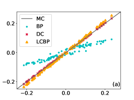
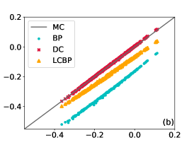
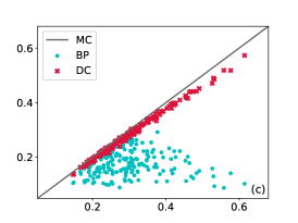
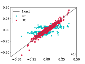
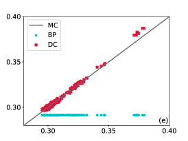
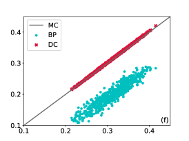
Figure 1: Comparison of DC, BP and LCBP on single-instances of disordered systems. (a) Magnetizations of AntiFerromagnetic Ising Model on a triangular lattice with $N=100,\left|E\right|=6N$, $J=-1$, $\beta=0.52$ and random binary fields of $|h_{i}|=0.2$. (b) Magnetization of Ferromagnetic Ising Model on a Random Regular (RR) Graph, $N=300$, degree $4$, $\beta=0.35$, $J=1$ and random binary fields of $|h_{i}|=0.3$. (c) Correlations of (heterogeneous) Ising Model on Barabasi-Albert graph, $N=100$, $n_{0}=k=2$ without external fields (the solution is found by using $\rho^{*}=0.95$ and it is divergent for $\rho>\rho^{*}$). (d) Magnetizations of a random $4-$SAT instance at $\alpha=\frac{M}{N}=4$ at $\beta\to\infty$. (e) Correlations of (heterogeneous) Ferromagnetic Ising Model on a Random Regular (RR) Graph, $N=300$, degree $4$ and $\beta=0.3$. (f) Correlations on a 3D hypercubic toroidal lattice ferromagnetic (heterogeneous) Ising Model, $N=6^{3}$ and $\beta=0.21$ and no external fields. In heterogeneous ferromagnetic models, couplings are drawn from a uniform distribution in $\left(0.5,1.5\right)$.

On acyclic factor graphs, the method converges in a finite number of iterations and is exact, i.e. on a fixed point, $\left\langle x_{i}\right\rangle_{g}$ equals to the magnetization $\left\langle x_{i}\right\rangle_{p}$. Therefore, as both the DC scheme and BP are exact on acyclic graphs, their estimation of marginals must coincide. However, a deeper connection can be pointed out. If a DC scheme applies zero covariances (e.g. by setting $\rho=0$ in (3)), on a DC fixed point on any factor graph the quantities $m_{ai}=\tanh\left(\mu_{i}^{a}/\Sigma_{ii}^{a}\right)$ satisfy the Belief Propagation (BP) equations. Moreover, DC follows dynamically a BP update. In particular, when equations converge, magnetizations $m_{i}=\tanh\left(\mu_{i}/\Sigma_{ii}\right)$ are equal to the corresponding belief magnetizations (Proof in A.1).

Interestingly, the DC scheme can be thought of as a Gaussian pairwise EP scheme with a modified consistency condition. The latter can be obtained by keeping (3) and replacing $\text{atanh}\left(x\right)$ in the RHS of (2) by the qualitatively similar $\frac{x}{1-x^{2}}$. This of course renders the method inexact on acyclic graphs and turns out to give generally a much worse approximation in many cases (See A.4). In addition, as it also happens with the EP method, Gaussian densities in factors $\psi_{a}$ can be moved freely between factors (sharing the same variables) without altering the approximation (details in A.3).

Numerical results

We tested the method on the Ising model on many different scenarios on heterogeneous systems, with a selection of results given in Figure 1. True values for magnetization and correlations were computed approximately with long Monte-Carlo runs ($1\times 10^{6}N-2\times 10^{6}N$ Monte-Carlo Gibbs-sampling steps) for Ising models and with the exact (exponential) trace for up to $N=28$ in the case of $k-$SAT. All simulations have been performed with a damping parameter $\text{around }0.95$ to improve convergence. The DC method provides a substantial correction to BP magnetizations and correlations in almost all cases ; it also improves single-node marginal estimates w.r.t. Loop Corrected Belief Propagation (LCBP) (Mooij et al., 2007) in several cases. LCBP simulations were performed using the code provided in (Mooij, 2010). We underline that, despite the computational cost per iteration of LCBP on bounded-degree graphs being $O\left(N^{2}\right)$, the prefactor depends strongly on the degree distribution (with even exponential scaling in some cases), also the number of iterations required to converge is normally much larger than the one of DC. For instance, for antiferromagnetic models (like the one shown in 1(a)), LCBP seems not to converge at smaller temperatures.

Homogeneous Ising model

Consider a homogeneous ferromagnetic Ising Model with coupling constant $J$ and external field $h^{ext}$ on on a $d$-dimensional lattice with periodic (toroidal) boundary condition: because of the translational invariance, all Gaussian factors $\phi_{a}$ are identical and the covariance matrix admits an analytic diagonalization. Therefore it is possible to estimate equilibrium observables through an analytical DC scheme also in the thermodynamic limit. After some calculations (see B.2), at a given temperature the DC solution is found by solving the following system of 3 fixed point equations $\sigma_{0}=\frac{m}{\text{atanh}m}$, $\sigma_{1}=\rho\frac{c-m^{2}}{1-m^{2}}\sigma_{0}$ and $y=m\left(\gamma_{0}+\gamma_{1}\right)$ in the Gaussian parameters $y,\gamma_{0},\gamma_{1}$ where $m=\left\langle x_{i}\right\rangle_{g^{\left(a\right)}}$, $c=\left\langle x_{i}x_{j}\right\rangle_{g^{\left(a\right)}}$ are the moments computed under the “tilted” distribution $g^{\left(a\right)}$, and $\sigma_{0},\sigma_{1},\gamma_{0},\gamma_{1}$ equal respectively $\Sigma_{ii},\Sigma_{ij},\left(2d\right)^{-1}\left(\Sigma^{-1}\right)_{ii},\left(\Sigma^{-1}\right)_{ij}$ for $i,j$ two first lattice neighbors. Defining $R_{d}\left(r\right)=\frac{1}{2}\int_{0}^{\infty}dte^{-dt}\mathcal{I}_{0}^{d}\left(rt\right)$, where $\mathcal{I}_{0}$ is the modified Bessel function of the first kind of order $0$, and after some straightforward algebraic manipulations, we finally obtain the following equations (here $h^{ext}=0$ for simplicity) for variable $\beta,m,r=\gamma_{1}\gamma_{0}^{-1}$

$$\beta= \text{atanh}\left[\frac{1}{\rho}k_{d}\left(r\right)\left(1-m^{2}\right)+m^{2}\right]-g_{d}\left(r\right)\frac{\text{atanh}m}{m}-\text{atanh}\left[\tanh^{2}\left(f_{d}\left(r\right)\text{atanh}m\right)\right]$$ (4)

$$m= \tanh\left[f_{d}\left(r\right)\text{atanh}m+\text{atanh}\left(\tanh\left(\beta+g_{d}\left(r\right)\frac{\text{atanh}m}{m}\right)\tanh\left(f_{d}\left(r\right)\text{atanh}m\right)\right)\right]$$ (5)

where $k_{d}\left(r\right)=\frac{1-2dR_{d}\left(r\right)}{r2dR_{d}\left(r\right)}$, $g_{d}\left(r\right)=\frac{k_{d}\left(r\right)}{1-k_{d}\left(r\right)^{2}}+rR_{d}\left(r\right)$, $f_{d}\left(r\right)=\frac{1}{1+k_{d}\left(r\right)}-\left(r+1\right)R_{d}\left(r\right)$. Substituting (4) into (5) we get a single equation for $m,r$, allowing for a parametric solution $m\left(r\right),\beta\left(r\right)$.

The maximum value of $\beta$ for which a paramagnetic solution exists can be analytically derived by substituting $m=0$ and taking $\sup_{-1<r\leq 0}\beta\left(r\right)$ from (4). For $d\geq 3$ the maximum is realized at $r=-1$, obtaining:

$$\beta_{p} =\text{ath}\left(1-\frac{1}{x_{d}}\right)-\frac{x_{d}\left(x_{d}-1\right)}{2x_{d}-1}+\frac{x_{d}}{2d}$$ (6)

where $x_{d}=2dR_{d}\left(-1\right)$. Values of $\beta_{p}$ for various dimensions $d$ are reported in table I. The paramagnetic solution is stable in the full range $0\leq\beta<\beta_{p}$ for $d\geq 3$.

Expanding (6) in powers of $d^{-1}$ we get $\frac{1}{2d\beta_{p}}=1-\frac{1}{2}d^{-1}-\frac{1}{3}d^{-2}-\frac{13}{24}d^{-3}-\frac{979}{720}d^{-4}-\frac{2039}{480}d^{-5}+O\left(d^{-6}\right)$ which is exact up to the $d^{-4}$ order (the correct coefficient of $d^{-5}$ is $-\frac{2009}{480}$) (Fisher and Gaunt, 1964). For comparison, nMF is exact up to the $d^{0}$ order, BP is exact up to the $d^{-1}$ order, and Loop Corrected Bethe (LCB, (Montanari and Rizzo, 2005)) and Plaquette CVM (PCVM, (Domínguez et al., 2017)) are exact up to the $d^{-2}$ order.

$d$	$\beta_{BP}$		$\beta_{PCVM}$		$\beta_{LCB}$		$\beta_{m}$		$\beta_{p}$		$\beta_{c}$
2	0.	34657	0.	412258	-		0.	388448	0.	37693	0.	440687
3	0.	20273	0.	216932	0.	238520	0.	218908	0.	222223	0.	221654(6)
4	0.	14384	0.	148033	0.	151650	0.	149835	0.	149862	0.	14966(3)
5	0.	11157	0.	113362	0.	114356	0.	113946	0.	113946	0.	11388(3)
6	0.	09116	0.	092088	0.	092446	0.	092304	0.	092304	(0.	0922530)

Table 1: Critical values obtained with different approximation schemes of the inverse temperature $\beta$ marking the onset of spontaneous magnetization in the homogeneous Ising model on infinite $d$-dimensional hypercubic lattices. The values of $\beta_{BP}$, $\beta_{PCVM}$ and $\beta_{LCB}$ respectively refer to the Bethe-Peierls, Plaquette Cluster Variational Method (Domínguez et al., 2017) and Loop Corrected Bethe (Montanari and Rizzo, 2005) approximations, while $\beta_{p}$ and $\beta_{m}$ respectively correspond to the maximum $\beta$ of the paramagnetic DC solution and the minimum $\beta$ of the magnetized DC solution, $\beta_{c}$ indicates the currently best known approximation up to numerical accuracy ((Domínguez et al., 2017) for $d\leq 5$, (Fisher and Gaunt, 1964) for $d=6$). Results in bold indicate the closest value to the last column.

The minimum value of $\beta$ for which a magnetized solution exists can be also computed by seeking a point with $\frac{d\beta}{dr}=0$ with the complication that $m$ is defined implicitly by (4)-(5) (details in B.2). The resulting equation has a single solution that has been numerically computed and shown in Table (1) as $\beta_{m}$. It turns out to be smaller but always very close to $\beta_{p}$ and coincident up to numerical precision for $d\geq 5$. Note that for inverse temperatures in the (albeit small) range $\beta_{m}<\beta<\beta_{p}$, the DC approximation has both magnetized and a paramagnetic stable solutions, suggesting a phase coexistence that should be absent in the real system (Lebowitz, 1977).

Discussion

We proposed a general approximation scheme for distributions of discrete variables that show interesting properties, including being exact on acyclic factor graphs and providing a form of loop corrections on graphs with cycles.

In the same spirit as for PCVM and LCBP, DC approximation can be thought of as a method to correct the cavity independence (or absence of cycles) assumption in the Bethe-Peierls approximation. Whereas PCVM deals only with local (short) cycles, it is true that LCBP and DC both attempt to correct for arbitrarily long cycles in the interaction graph. However, they do so through crucially different approaches. Loop Corrected Belief Propagation (LCBP) works by computing several BP fixed points (one for each cavity distribution in which one node and all the factors connected to it are removed) and then imposing consistency over single-node beliefs among them. Therefore, for each cavity distribution it computes fixed points by still assuming a tree-factorization, i.e. by neglecting correlations coming from other cycles in the graph. So it computes a higher order approximation by relying on lower order ones (on a modified/simplified) interaction graph. In this sense, it can be considered as a first-order correction to BP and indeed it improves BP estimates of single-node marginals, as shown in 1. In this perspective, DC can be considered as a new approximation in which all 2-points cavity correlations are taken into account (of course, in an approximate way, through a Gaussian distribution), in a single self-consistent set of equations in which correlations arise simultaneously from all cycles in the graph.

The method can be in part solved analytically on homogeneous systems such as finite dimensional hypercubic lattices with periodic conditions. Analytical predictions from the model show a number of interesting features that are not shared by other mean-field approaches: the method provides finite size corrections which are in close agreement with numerical simulations; the paramagnetic solution exists only for $\beta<\beta_{p}$ (in PCVM and BP, the paramagnetic solution exists for all $\beta\geq 0$, although it stops being stable at a finite value of $\beta$); it can capture some types of heterogeneity where the Bethe-Peierls approximation can not (such as in RR graphs). Numerical simulations are in good agreement on different models, including random-field Ising with various topologies and random $k-$SAT. On lattices, the method could in principle be rendered more accurate by taking into account small loops explicitly. The DC scheme can be extended for models with $q-$states variables, by replacing each of them with $q$ binary variables. Again, in this setup it is possible to get a similar set of closure equations that are exact on acyclic graphs and recover BP fixed points on any graph when neglecting cavity correlations. This will be object of future research.

Appendix A General properties of DC scheme

A.1 Relation with the Bethe Approximation (BP)

On acyclic graphs, both the DC scheme and BP are exact and thus they must coincide on their computation of marginals. However, a deeper connection can be pointed out. BP fixed point equations are

$$m_{ai}\left(x_{i}\right)\propto \sum_{\boldsymbol{x}_{a}}\psi_{a}\left(x_{a}\right)\prod_{j\in a\setminus i}m_{ja}\left(x_{j}\right)$$ (7)

$$m_{ia}\left(x_{i}\right)\propto \prod_{b\in i\setminus a}m_{bi}\left(x_{i}\right)$$ (8)

$$m_{i}\left(x_{i}\right)\propto \prod_{b\in i}m_{bi}\left(x_{i}\right)$$ (9)

Theorem 1.

If (H1) the DC scheme applies zero covariances or (H2) the factor graph is acyclic, $m_{ia}\left(x_{i}\right)\propto g^{-a}\left(x_{i}\right)$ satisfies (7)-(8). Moreover, the updates follow dynamically BP updates. In particular, if equations converge, approximate marginals $g\left(x_{i}\right)$ are proportional to belief magnetizations (9).

Proof.

In the either hypothesis (H1 or H2) , $g^{-a}\left(x_{a}\right)\propto\prod_{j\in\partial a}m_{ja}\left(x_{j}\right)$. Define $m_{ai}\left(x_{i}\right)\propto\frac{g\left(x_{i}\right)}{m_{ia}\left(x_{i}\right)}$. We obtain

$$m_{ai}\left(x_{i}\right) \propto\frac{1}{m_{ia}\left(x_{i}\right)}\int dx_{a\setminus i}g\left(x_{a}\right)$$

$$\propto\int dx_{a\setminus i}\prod_{j\in\partial a\setminus i}m_{ja}\left(x_{j}\right)\phi_{a}\left(x_{a}\right)$$ (10)

Thanks to (2), $g\left(x_{i}\right)\propto g^{\left(a\right)}\left(x_{i}\right)$ when $x_{i}\in\left\{-1,1\right\}$ (and this is precisely the purpose of (2)). In particular, for $x_{i}\in\left\{-1,1\right\}$ we get also

$$m_{ai}\left(x_{i}\right) \propto\frac{1}{m_{ia}\left(x_{i}\right)}g^{\left(a\right)}\left(x_{i}\right)$$

$$=\frac{1}{m_{ia}\left(x_{i}\right)}\sum_{x_{a\setminus i}}g^{-a}\left(x_{a}\right)\psi_{a}\left(x_{a}\right)$$

$$=\sum_{x_{a\setminus i}}\prod_{j\in\partial a\setminus i}m_{ja}\left(x_{j}\right)\psi_{a}\left(x_{a}\right)$$ (11)

which is Eq. (7). Eq. (8) is also verified in either hypothesis:

1. Factorized case: if $\phi_{a}\left(x_{a}\right)=\prod_{i\in\partial a}\phi_{a}\left(x_{i}\right)$, then clearly $m_{ai}\left(x_{i}\right)\propto\phi_{a}\left(x_{i}\right)$ and $m_{ia}\left(x_{i}\right)\propto\prod_{b\in\partial i\setminus a}m_{bi}\left(x_{i}\right)$

2. Acyclic case: if $T_{b}$ denotes the set of factors in the connected component of $b$ once $i$ is removed, we get

   $$m_{ia}\left(x_{i}\right) \propto g^{-a}\left(x_{i}\right)$$

   $$\propto\int dx_{-i}\prod_{b\in\partial i\setminus a}\phi_{b}\left(x_{b}\right)\prod_{c\in T_{b}\setminus b}\phi_{c}\left(x_{c}\right)$$

   $$\propto\prod_{b\in\partial i\setminus a}\int dx_{b\setminus i}\phi_{b}\left(x_{b}\right)\prod_{j\in\partial b\setminus i}g^{-b}\left(x_{j}\right)$$

   $$\propto\prod_{b\in\partial i\setminus a}\int dx_{b\setminus i}\phi_{b}\left(x_{b}\right)\prod_{j\in\partial b\setminus i}m_{bj}\left(x_{j}\right)$$

   $$\propto\prod_{b\in\partial i\setminus a}m_{bi}\left(x_{i}\right)$$ (12)

   where the last line follows from (10).

∎

A.2 Relation with EP

The DC scheme can be thought of a modified Gaussian EP scheme for factors

$$\hat{\psi}_{ij}\left(x_{i},x_{j}\right)=\psi_{ij}\left(x_{i},x_{j}\right)\left(\delta\left(x_{i}+1\right)+\delta\left(x_{i}-1\right)\right)\left(\delta\left(x_{i}+1\right)+\delta\left(x_{i}-1\right)\right)$$

Classic EP equations in this context can be obtained by replacing $\text{atanh}\left\langle x_{i}\right\rangle_{g^{\left(a\right)}}$ in the RHS of (2) by the qualitatively similar function $\frac{\left\langle x_{i}\right\rangle_{g^{\left(a\right)}}}{1-\left\langle x_{i}\right\rangle_{g^{\left(a\right)}}^{2}}$, but this of course invalidates Theorems 1-2 and turns out to give a much worse approximation in general.

A.3 Weight gauge

One interesting property common to both DC and EP scheme concerns the possibility to move freely gaussian densities in and out the exact factors $\psi_{a}\left(x_{a}\right).$ Let $\rho_{a}\left(x_{a}\right)$ be Gaussian densities;

$$p\left(x\right) \propto g\left(x\right)\prod_{a}\psi_{a}\left(x_{a}\right)$$

$$q\left(x\right) \propto g\left(x\right)\prod_{a}\phi_{a}\left(x_{a}\right)$$

and $q$ a Gaussian EP or DC approximation. We have

$$p^{\left(a\right)}\left(x_{a}\right) \propto\psi_{a}\left(x_{a}\right)\int dx_{-a}\frac{g\left(x\right)\prod_{b}\phi_{b}\left(x_{b}\right)}{\phi_{a}\left(x_{a}\right)}$$ (13)

$$\propto\frac{\psi_{a}\left(x_{a}\right)}{\rho_{a}\left(x_{a}\right)}\int dx_{-a}\frac{\left[g\left(x\right)\prod_{b}\rho_{b}\left(x_{b}\right)\right]\prod_{b}\phi_{b}\left(x_{b}\right)/\rho_{b}\left(x_{b}\right)}{\phi_{a}\left(x_{a}\right)/\rho_{a}\left(x_{a}\right)}$$ (14)

$$q\left(x_{a}\right) =\int dx_{-a}g\left(x\right)\prod_{b}\phi_{b}\left(x_{b}\right)$$ (15)

$$=\int dx_{-a}\left[g\left(x\right)\prod_{b}\rho_{b}\left(x_{b}\right)\right]\prod_{b}\phi_{b}\left(x_{b}\right)/\rho_{b}\left(x_{b}\right)$$ (16)

As DC and EP algorithms impose constraints between $p^{\left(a\right)}\left(x_{a}\right)$ and $q\left(x_{a}\right)$, any approximating family $\left\{\phi_{a}\right\}$ for $\left(g,\left\{\psi_{a}\right\}\right)$ leads to an equivalent family $\left\{\phi_{a}/\rho_{a}\right\}$ for $\left(g^{\prime}=g\prod_{b}\rho_{b},\left\{\psi^{\prime}_{a}=\psi_{a}/\rho_{a}\right\}\right)$ for arbitrary factors $\rho_{a}$.

A.4 Other closure equations

Eq. 2 is the only condition needed to make the approximation scheme exact on tree-graphs. In principle one could complement it with any other condition in order to obtain a well-determined system of equations and unknowns in the factor parameters. In this work we tried other complementary closure equations (including matching of covariance matrix, constrained Kullback-Leiber Divergence minimization, matching of off-diagonal covariances, in addition to 2). However, we found out that 3 were experimentally performing uniformly better on all the cases we analyzed.

Appendix B Homogeneous Ising Model

In a homogeneous ferromagnetic Ising Model with hamiltonian $\mathcal{H}=-J\sum_{\langle i,j\rangle}x_{i}x_{j}-h^{ext}\sum_{i}x_{i}$ defined on a $d$-dimensional hypercubic lattice with periodic (toroidal) boundary condition, all Gaussian factors $\phi_{a}$ are identical and the DC equations (32) at a given inverse temperature $\beta$ read:

$$\sigma_{0} =\frac{m}{\text{atanh}m}$$

$$\sigma_{1} =\rho\frac{c-m^{2}}{1-m^{2}}\sigma_{0}$$ (17)

$$y =m\left(\gamma_{0}+\gamma_{1}\right)$$

The DC solution is found by solving the above system of 3 fixed-point equations in the Gaussian parameters $y,\gamma_{0},\gamma_{1}$ where $\sigma_{0},\sigma_{1},\gamma_{0},\gamma_{1}$ equal respectively $\Sigma_{ii}$, $\Sigma_{ij}$, $\left(2d\right)^{-1}$$\left(\Sigma^{-1}\right)_{ii}$, $\left(\Sigma^{-1}\right)_{ij}$ for $i,j$ two first lattice neighbors. Here $m=\left\langle x_{i}\right\rangle_{g^{\left(a\right)}}$ and $c=\left\langle x_{i}x_{j}\right\rangle_{g^{\left(a\right)}}$ are the moments computed under the distribution $g^{\left(a\right)}$:

$$m =\tanh\left[z+\text{atanh}\left(\tanh\Gamma\tanh z\right)\right]$$

$$c =\tanh\left[\Gamma+\text{atanh}\left(\tanh^{2}z\right)\right]$$

where

$$z =\frac{\beta h^{ext}}{2d}+\left(\frac{1}{\sigma_{0}+\sigma_{1}}\frac{1}{\gamma_{0}+\gamma_{1}}-1\right)y$$

$$\Gamma =\beta J+\frac{\sigma_{1}}{\sigma_{0}^{2}-\sigma_{1}^{2}}+\gamma_{1}$$

The matrix $\Sigma$ is the gaussian covariance matrix whose inverse is parametrized as follows:

$$\Sigma^{-1}=\mathcal{S}^{\left(d\right)}=2d\gamma_{0}\mathbb{I}_{L^{d}}+\gamma_{1}\mathcal{A}^{\left(d\right)}$$

where $\mathcal{A}^{\left(d\right)}$ is the lattice adjacency matrix in dimension $d$, whose diagonalization is discussed in the next section.

B.1 Diagonalization of $A^{\left(d\right)}$

The hypercubic lattice in $d$ dimensions can be regarded as the cartesian product of linear-chain graphs, one for each dimension. The adiacency matrix of the whole lattice can be thus expressed as function of the adiacency matrices of the single linear chains, by means of the Kronecker product (indicated by $\otimes$):

$$\mathcal{A}^{\left(d\right)}=\mathcal{A}^{\left(1\right)}\otimes\mathcal{\mathbb{I}}_{L}\otimes...\mathcal{\otimes\mathbb{I}}_{L}+\mathbb{I}_{L}\otimes\mathcal{A}^{\left(1\right)}\otimes\mathbb{I}_{L}\otimes...\mathbb{I}_{L}+...+\mathbb{I}_{L}\otimes...\otimes\mathbb{I}_{L}\otimes\mathcal{A}^{\left(1\right)}$$

where $\mathcal{A}^{\left(1\right)}$ is the adiacency matrix of a (closed) linear chain of size $L$:

$$\mathcal{A}^{\left(1\right)}=\begin{bmatrix}0&1&0&\cdots&0&0&1\\ 1&0&1&\cdots&0&0&0\\ 0&1&0&\cdots&0&0&0\\ \vdots&\vdots&\vdots&\ddots&\vdots&\vdots&\vdots\\ 0&0&0&\cdots&0&1&0\\ 0&0&0&\cdots&1&0&1\\ 1&0&0&\cdots&0&1&0\end{bmatrix}$$

The above expression allows to compute the spectral decomposition of $\mathcal{A}^{\left(d\right)}$ just by knowing the spectrum of the adiacency matrix of the linear chain. The matrix $\mathcal{A}^{\left(1\right)}$ is a special kind of circulant matrix and therefore it can be diagonalized exactly [Davis, 1979]. Its eigenvalues and eigenvectors are shown below:

$$\lambda_{x}^{\left(1\right)}=2\textnormal{cos}\left(\frac{2\pi}{L}x\right)\qquad\qquad\nu_{x}^{\left(1\right)}=\frac{1}{\sqrt{L}}\left(1,w_{x},w_{x}^{2},\ldots,w_{x}^{L-1}\right)$$

where $x\in\left\{0,...,L-1\right\}$ and $w_{x}=e^{i\frac{2\pi}{L}x}$.

The spectral decomposition of $\mathcal{A}^{(d)}$ reads:

$$\lambda_{\left(x_{1},\ldots,x_{d}\right)}^{(d)} =\sum_{j=1}^{d}\lambda_{x_{j}}^{\left(1\right)}=2\sum_{j=1}^{d}\textnormal{cos}\left(\frac{2\pi}{L}x_{j}\right)$$ (18)

$$\nu_{\left(x_{1},\ldots x_{d}\right)} =\varotimes_{j=1}^{d}\nu_{x_{j}}^{\left(1\right)}$$ (19)

We recall now the expression of the eigenvalues of $S^{\left(d\right)}$:

$$\lambda_{\left(x_{1},\ldots,x_{d}\right)}=2d\gamma_{0}+2\gamma_{1}\sum_{j=1}^{d}\textnormal{cos}\left(\frac{2\pi}{L}x_{j}\right)$$

The inverse matrix elements $\Sigma_{ii},\Sigma_{ij}$ can be computed in a straightfoward way. In particular, in the thermodynamic limit $\left(L\to\infty\right)$ their expressions read:

$$\sigma_{0} =\frac{1}{\gamma_{0}}R\left(r\right)$$ (20)

$$\sigma_{1} =\frac{1}{\gamma_{0}r}\left[\frac{1}{2d}-R\left(r\right)\right]$$ (21)

where $r=\frac{\gamma_{1}}{\gamma_{0}}$ and $R_{d}\left(r\right)=\frac{1}{2}\int_{0}^{\infty}dte^{-dt}\left[\mathcal{I}_{0}\left(rt\right)\right]^{d}$, where $\mathcal{I}_{0}$ is the modified Bessel function of the first kind of order $0$.

B.2 Simplified DC equations

It is possible to simplify the original system (17) in order to get a fixed point equation for the magnetization $m$. By eliminating the variable $y$ and setting $J=1$ we get

$$z= m\left(\frac{1}{\sigma_{0}+\sigma_{1}}-\left(\gamma_{0}+\gamma_{1}\right)\right)+\frac{\beta}{2d}h^{ext}$$

$$= m\gamma_{0}\left(\frac{1}{R_{d}\left(r\right)+\frac{1}{r}\left[\frac{1}{2d}-R_{d}\left(r\right)\right]}-r-1\right)+\frac{\beta}{2d}h^{ext}$$ (22)

$$\Gamma= \beta+\frac{\sigma_{1}}{\sigma_{0}^{2}-\sigma_{1}^{2}}+r\gamma_{0}$$

$$= \beta+\gamma_{0}\left(\frac{\frac{1}{r}\left(\frac{1}{2d}-R_{d}\left(r\right)\right)}{R_{d}^{2}\left(r\right)-\frac{1}{r^{2}}\left[\frac{1}{2d}-R_{d}\left(r\right)\right]^{2}}+r\right)$$ (23)

Now, putting together Eq.(17) with Eq.(22)-(23) and the definitions (20)-(21) we get the following system:

$$\beta= \text{atanh}\left[\frac{1}{\rho}k_{d}\left(r\right)\left(1-m^{2}\right)+m^{2}\right]-g_{d}\left(r\right)\frac{\text{atanh}m}{m}-\text{atanh}\left[\tanh^{2}\left(f_{d}\left(r\right)\text{atanh}m+\frac{\beta}{2d}h^{ext}\right)\right]$$ (24)

$$m= \tanh\bigg{[}f_{d}\left(r\right)\text{atanh}m+\frac{\beta}{2d}h^{ext}+$$ (25)

$$+\text{atanh}\left(\tanh\left(\beta+g_{d}\left(r\right)\frac{\text{atanh}m}{m}\right)\tanh\left(f_{d}\left(r\right)\text{atanh}m+\frac{\beta}{2d}h^{ext}\right)\right)\bigg{]}$$

where $k_{d}\left(r\right)=\frac{1-2dR_{d}\left(r\right)}{2drR_{d}\left(r\right)}$, $g_{d}\left(r\right)=\frac{k_{d}\left(r\right)}{1-k_{d}\left(r\right)^{2}}+rR_{d}\left(r\right)$, $f_{d}\left(r\right)=\frac{1}{1+k_{d}\left(r\right)}-\left(r+1\right)R_{d}\left(r\right)$. Such equations can be solved at fixed $r$ in the variables $\beta,m$. For $h=0$ the system reduces to a single fixed point equation for $m=M\left(m\left(r\right),r\right)$ while $\beta$ is fixed by (24).

Computation of $\beta_{p}$

For the paramagnetic solution $m=0$ (with $h=0$) we get the following equation for $\beta\left(r\right)$:

$$\beta= \text{atanh}\left(\frac{1}{\rho r}\left[\frac{1}{2dR_{d}\left(r\right)}-1\right]\right)-g\left(r\right)$$

For $d\geq 3$, the maximum value at which a paramagnetic solution exists corresponds to the point $r=-1$. Therefore, the value of the critical point $\beta_{p}$ is computed by taking the $r\to-1$ limit of Eq.(24):

$$\beta_{p}= \text{atanh}\left(1-\frac{1}{z}\right)-z\left(\frac{z-1}{2z-1}\right)+\frac{z}{2d}$$ (26)

with $z=2dR_{d}\left(-1\right).$

Computation of $\beta_{m}$

Eqs. (24)-(25) implicitly define a function $m\left(r\right)$ such that $M\left(m\left(r\right),r\right)=m$, and thus also $\beta\left(r\right)=\beta\left(m\left(r\right),r\right)$. We seek to find the point $m^{*}=m\left(r^{*}\right)$ and $\beta_{m}=\beta\left(m^{*},r^{*}\right)$ such that $\frac{d\beta}{dr}\left(m\left(r^{*}\right),r^{*}\right)=0$. Taking the total derivative of $\beta\left(m\left(r\right),r\right)$ we get the equation to be solved

$$0=\frac{d\beta}{dr}=\frac{\partial\beta}{\partial r}+\frac{\partial\beta}{\partial m}\frac{dm}{dr}$$

To compute $\frac{dm}{dr}$ we use its implicit definition,

$$0 =\frac{d}{dr}\left\{M\left(m\left(r\right),r\right)-m\left(r\right)\right\}$$

$$=\left(\frac{\partial M}{\partial m}\left(m\left(r\right),r\right)-1\right)\frac{dm}{dr}+\frac{\partial M}{\partial r}\left(m\left(r\right),r\right)$$

$$\frac{dm}{dr} =-\frac{\frac{\partial M}{\partial r}\left(m\left(r\right),r\right)}{\frac{\partial M}{\partial m}\left(m\left(r\right),r\right)-1}$$

to get finally the $2\times 2$ system in variables $m,r$:

$$M\left(m,r\right)-m =0$$ (27)

$$\frac{\partial\beta}{\partial r}\left(m,r\right)\left(\frac{\partial M}{\partial m}\left(m,r\right)-1\right)-\frac{\partial M}{\partial r}\left(m,r\right)\frac{\partial\beta}{\partial m}\left(m,r\right) =0$$ (28)

Stability

The stability of a fixed point $m^{*}=m\left(r^{*}\right)$ can be analyzed by computing $\frac{dM}{dm}\bigg{|}_{m^{*}}$. In particular, starting from the system (24)-(25) where $r$ is implicitly defined as $r=R\left(\beta,m\right),$the instability occurs when $\frac{dM}{dm}\bigg{|}_{m^{*}}=1$. Writing the original system using the definition of $r$ we get $m=M\left(m,R\left(\beta,m\right)\right)$ and $\beta=B\left(m,R\left(\beta,m\right)\right)$. The equation we want to solve is

$$1 =\frac{dM}{dm}=\frac{\partial M}{\partial m}+\frac{\partial M}{\partial r}\frac{\partial R}{\partial m}$$

To compute $\frac{\partial R}{\partial m}$ we use again its implicit definition:

$$0 =\frac{\partial B}{\partial m}+\frac{\partial B}{\partial r}\frac{\partial R}{\partial m}$$

$$\frac{\partial R}{\partial m} =-\frac{\frac{\partial B}{\partial m}}{\frac{\partial B}{\partial r}}$$

The final system to solve is

$$M\left(m,r\right)-m =0$$ (29)

$$\frac{\partial M}{\partial m}-\frac{\partial M}{\partial r}\frac{\frac{\partial B}{\partial m}}{\frac{\partial B}{\partial r}} =1$$ (30)

For $d\geq 3$, the solution becomes unstable exactly at the point $\left(r_{m},\beta_{m}\right)$ computed through 27-28.

B.3 D=2

On a 2-dimensional square lattice, the DC solution is qualitatively different w.r.t. $d\geq 3$ because the function $R\left(r\right)$ is logarithmically divergent for $r\to-1$. In such case the maximum value at which the paramagnetic solution exists $\left(\beta_{p}=0.37693\right)$ corresponds to the point $r_{p}=-0.994843$. The ferromagnetic solution turns out to be stable for $r_{m}<r<0$ with $r_{m}=-0.99405$, corresponding to $\beta_{m}=0.388448$ (the point $\left(r_{m},\beta_{m}\right)$ is found as a solution of Eq. 29-30). Therefore there exists a temperature interval $\beta_{p}<\beta<\beta_{m}$ in which no stable DC solution can be found.

For finite size lattices the DC solution can still be found numerically, showing similar performances with respect to CVM on both ferromagnetic and spin glass models (Fig. 2). However, especially on ferromagnetic systems DC solution is numerically unstable close to the transition $\beta_{p}$. One way to reduce numerical instability in such region is to decrease the interpolation parameter $\rho$, typically fixed to 1 for DC. Neverthless, the meaning of the DC($\rho$) approximation in this case is not clear.

Figure 2: Left: distribution of non-overlapping plaquettes (in grey) on a 2-dimensional square lattice. Right: correlations on 2-dimensional Ising Model on square lattice of size $L=10$ at $\beta=0.36$, with $0$ external field and couplings drawn from a uniform distribution in $\left(0.5,1.5\right)$. Comparison of DC, pDC, BP and CVM

One possible way to improve the DC approximation is to take into account small loops explicitly. In particular, we consider a gaussian family of approximating distribution factorized over plaquettes of $2^{d}$spins ($d$ is the number of dimensions). Plaquettes are chosen in such a way that there is no overlap between links in the gaussian distribution. In this way, DC equation are exact on a plaquette tree with only site-overlaps. Results are shown in 2: plaquette-DC (pDC) is in general slighty better than standard DC and comparable to CVM.

B.4 Finite size corrections

In homogeneous models the gaussian covariance matrix can be diagonalized analytically even for a finite size lattice (of size $L$). Therefore we can compute finite size corrections to the DC solution at a fixed $\beta$, as shown in the following plot:

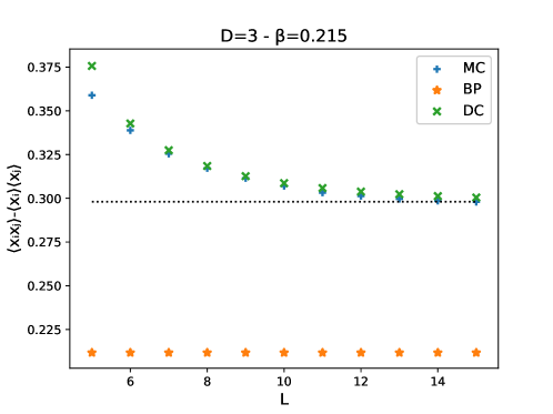
Figure 3: Finite size correction of equilibrium correlations at $\beta=0.215$ on a 3-dimensional cubic lattice of size $L\in\left\{5,...,15\right\}$ with $h=0,J=1$. Comparison of BP and DC solutions with Monte-Carlo simulations.

DC solution turns out to be in good agreement with MC results; on the other hand, BP does not take into account at all finite size corrections because of the local character of the approximation.

B.5 Scaling of $\beta_{c}$ in the high dimensional limit

Starting from the expression of the critical inverse temperature $\beta_{p}$ it is possible to compute the $1/d$ expansion in the high-dimensional limit. We recall the expression of the critical temperature (26):

$$\beta_{p}= \text{atanh}\left(1-\frac{1}{z}\right)-z\left(\frac{z-1}{2z-1}\right)+\frac{z}{2d}$$

where $z=2dR_{d}\left(-1\right)$.

Defining $x=1/d$ and expanding around $x=0$ we get:

$$\frac{1}{2d\beta_{p}}=1-\frac{1}{2}d^{-1}-\frac{1}{3}d^{-2}-\frac{13}{24}d^{-3}-\frac{979}{720}d^{-4}-\frac{2039}{480}d^{-5}+O\left(d^{-6}\right).$$

This expansion is exact up to the $d^{-4}$ order (the correct coefficient of $d^{-5}$ is $-\frac{2009}{480}$) (Fisher and Gaunt, 1964). For comparison, Mean Field is exact up to the $d^{0}$ order, Bethe is exact up to the $d^{-1}$ order, and Loop-Corrected Bethe and Plaquette-CVM are exact up to the $d^{-2}$ order.

For the sake of completeness, we report the series expansion of $R_{d}\left(-1\right)$ around $x=0$:

$$R_{d}\left(-1\right)=\frac{1}{2}d^{-1}+\frac{1}{4}d^{-2}+\frac{3}{8}d^{-3}+\frac{3}{4}d^{-4}+\frac{15}{8}d^{-5}+\frac{355}{64}d^{-6}+\frac{595}{32}d^{-7}+O\left(d^{-8}\right)$$

Appendix C Multistates variables

The method we presented is based on the possibility to fit the probability values of a discrete binary distribution with the density values of a univariate gaussian on the same support. When the model variables take $q>2$ values there is no general way to fit single-node marginals with a univariate Gaussian distribution. One possible solution is to replace each $q$-state variable $x_{i}$ with a vector of $q$ (correlated) binary variables $\boldsymbol{s^{i}}$, where $s_{\alpha}^{i}\in\left\{-1,1\right\}\forall\alpha=1,..,q$, with the following constraint:

$$\sum_{\alpha=1}^{q}s_{\alpha}^{i}=2-q$$

In this way, for each node $i$, only configurations of the type $\boldsymbol{s}^{i}=\left\{1,-1,...,-1\right\}$ (and its permutations) are allowed, in order to select just one of the $q$ states for $x_{i}$. For each factor node a, such constraints can be implemented by adding a set of delta functions in the original probability distribution, which is now a function of the new binary variables $\boldsymbol{s}^{i}$. The correlations induced by these constraints on the spin components of each $\boldsymbol{s^{i}}$ introduce short loops even when the original graph is a tree. Neverthless, it is still possible to write a set of matching equation similar to the 2-states case which is exact on trees.

References

• Lauritzen (1996) S. L. Lauritzen, Graphical models, Vol. 17 (Clarendon Press, 1996).
• MacKay (2003) D. J. MacKay, Information theory, inference and learning algorithms (Cambridge university press, 2003).
• Opper et al. (2001) M. Opper, O. Winther, et al., Advanced mean field methods: theory and practice , 7 (2001).
• Mezard and Montanari (2009) M. Mezard and A. Montanari, Information, physics, and computation (Oxford University Press, 2009).
• Berrou et al. (1993) C. Berrou, A. Glavieux,  and P. Thitimajshima, in Proceedings of ICC ’93 - IEEE International Conference on Communications, Vol. 2 (1993) pp. 1064–1070 vol.2.
• Kikuchi (1951) R. Kikuchi, Physical review 81, 988 (1951).
• Yedidia et al. (2003) J. S. Yedidia, W. T. Freeman,  and Y. Weiss, Exploring artificial intelligence in the new millennium 8, 236 (2003).
• Pelizzola (2005) A. Pelizzola, Journal of Physics A: Mathematical and General 38, R309 (2005).
• Chertkov and Chernyak (2006) M. Chertkov and V. Y. Chernyak, Journal of Statistical Mechanics: Theory and Experiment 2006, P06009 (2006).
• Gómez et al. (2007) V. Gómez, J. M. Mooij,  and H. J. Kappen, Journal of Machine Learning Research 8, 1987 (2007).
• Parisi and Slanina (2006) G. Parisi and F. Slanina, Journal of Statistical Mechanics: Theory and Experiment 2006, L02003 (2006).
• Altieri et al. (2017) A. Altieri, M. C. Angelini, C. Lucibello, G. Parisi, F. Ricci-Tersenghi,  and T. Rizzo, Journal of Statistical Mechanics: Theory and Experiment 2017, 113303 (2017).
• Montanari and Rizzo (2005) A. Montanari and T. Rizzo, J. Stat. Mech. 2005, P10011 (2005).
• Mooij et al. (2007) J. Mooij, B. Wemmenhove, B. Kappen,  and T. Rizzo, in Artificial Intelligence and Statistics (2007) pp. 331–338.
• Rizzo et al. (2007) T. Rizzo, B. Wemmenhove,  and H. J. Kappen, Physical Review E 76, 011102 (2007).
• Ohzeki (2013) M. Ohzeki, in Journal of Physics: Conference Series, Vol. 473 (IOP Publishing, 2013) p. 012005.
• Minka (2001) T. P. Minka, in Proceedings of the Seventeenth Conference on Uncertainty in Artificial Intelligence, UAI’01 (Morgan Kaufmann Publishers Inc., San Francisco, CA, USA, 2001) pp. 362–369.
• Opper and Winther (2001) M. Opper and O. Winther, Physical Review E 64, 056131 (2001).
• Opper and Winther (2005) M. Opper and O. Winther, The Journal of Machine Learning Research 6, 2177 (2005).
• Mooij (2010) J. M. Mooij, Journal of Machine Learning Research 11, 2169 (2010).
• Note (1) $R_{2}\left(-1\right)$ is divergent and the maximum for $d=2$ is located in $-1<r^{*}<0$. The solution for $d=2$ is thus qualitatively different, see B.3.
• Fisher and Gaunt (1964) M. E. Fisher and D. S. Gaunt, Phys. Rev. 133, A224 (1964).
• Domínguez et al. (2017) E. Domínguez, A. Lage-Castellanos, R. Mulet,  and F. Ricci-Tersenghi, Phys. Rev. E 95, 043308 (2017).
• Lebowitz (1977) J. L. Lebowitz, J Stat Phys 16, 463 (1977).
• Note (2) With the apparent ambiguity of the appearance of $\delta^{k}$ terms in $p\left(x\right)$, which is actually really not as problematic as it may seem as the distribution is defined up to a normalization factor; more precisely consider
p(x)=limσ01Zσ\prod@\slimits@ij\mathaccentVhat05Eψσ,ij(xi,xj)𝑝𝑥subscript𝑙𝑖𝑚𝜎01subscript𝑍𝜎\prod@subscript\slimits@similar-to𝑖𝑗\mathaccentV𝑎𝑡05𝐸subscript𝜓𝜎𝑖𝑗subscript𝑥𝑖subscript𝑥𝑗p\left(x\right)=\mathop{lim}\displaylimits_{\sigma\to 0}\frac{1}{Z_{\sigma}}\prod@\slimits@_{i\sim j}\mathaccentV{hat}05E{\psi}_{\sigma,ij}\left(x_{i},x_{j}\right)
for factors $\mathaccentV{hat}05E{\psi}_{\sigma,ij}\left(x_{i},x_{j}\right)=\psi_{ij}\left(x_{i},x_{j}\right)\left(\mathcal{N}\left(x_{i};1,\sigma\right)+\mathcal{N}\left(x_{i};-1,\sigma\right)\right)\left(\mathcal{N}\left(x_{j};1,\sigma\right)+\mathcal{N}\left(x_{j};-1,\sigma\right)\right)$.
• Davis (1979) P. J. Davis, Circulant Matrices (1979).