Exchangeable Markov multi-state survival processes

Abstract

We consider exchangeable Markov multi-state survival processes – temporal processes taking values over a state-space $\mathcal{S}$ with at least one absorbing failure state $\flat\in\mathcal{S}$ that satisfy natural invariance properties of exchangeability and consistency under subsampling. The set of processes contains many well-known examples from health and epidemiology – survival, illness-death, competing risk, and comorbidity processes; an extension leads to recurrent event processes.

We characterize exchangeable Markov multi-state survival processes in both discrete and continuous time. Statistical considerations impose natural constraints on the space of models appropriate for applied work. In particular, we describe constraints arising from the notion of composable systems. We end with an application of the developed models to irregularly sampled and potentially censored multi-state survival data, developing a Markov chain Monte Carlo algorithm for posterior computation.

1 Introduction

In many clinical survival studies, a recruited patient’s health status is monitored on either a regular or intermittent schedule until either (1) an event of interest (e.g., failure) or (2) the end of the study window. Covariates are recorded at the time of recruitment, and treatment protocols per patient are presumed known at baseline. In the simplest survival study, health status $Y(t)$ at time $t$ is a binary variable, dead $(0)$ or alive $(1)$. In clinical trials with health monitoring, $Y(t)$ is a more detailed description of the state of health of the individual, containing relevant patient information, e.g., pulse rate, cholesterol level, cognitive score or CD4 cell count (Diggle et al., 2008; Farewell and Henderson, 2010; Kurland et al., 2009).

In this paper, we consider the setting in which the health process takes values in some pre-specified “state-space”. For example, in the illness-death model, we summarize the current state of the participant as taking one of three possible values $\{\text{Healthy, Ill, Dead}\}$. Such a process can be thought of as a coarse view of the state of health for a patient over time. The continuing importance of multi-state processes in applications cannot be overstated (Jepsen et al., 2015; van den Hout, 2016).

When no baseline covariates are measured beyond the initial state $Y(0)$, the model for the set of patient state-space processes should satisfy natural constraints. First, the model should be agnostic to patient labeling. Second, the model should be agnostic to sample size considerations. These natural constraints (mathematically defined in section 2) lead to the concept of exchangeable Markov multi-state survival processes. The purpose of this paper is to characterize the set of multi-state survival processes and show how this theory of exchangeable stochastic processes fits naturally into the applied framework of event-history analysis. Both the parametric continuous-time Markov process with independent participants and the nonparametric counting process are contained as limiting cases. Next, we discuss the notion of “composable systems” and its effect on model specification. A Markov Chain Monte Carlo (MCMC) algorithm is then derived for posterior computations given irregularly sampled multi-state survival data. We end with an application to a cardiac allograft vasculopathy (CAV) multi-state survival study.

1.1 Related work

Odd Aalen was one of the first to recognize the importance of incorporating the “theory of stochastic processes” into an “applied framework of event history analysis” (Aalen et al., 2008, p. 457). Martingales and counting processes form the basis of this nonparametric approach. The fundamental concept of the product-integral unifies discrete and continuous-time processes. Nonparametric methods, however, do not adequately handle intermittent observations. For example, Aalen et al. (2015) consider dynamic path analysis for a liver cirrhosis dataset. In this study, the prothrombin index, a composite blood coagulation index related to liver function, is measured initially at three-month intervals and subsequently at roughly twelve-month intervals. To deal with the intermittency of observation times, Aalen et al. (2015) use the “last-observation carried forward” (LOCF) assumption. However, such an assumption is unsatisfactory for highly variable health processes, and can lead to biased estimates (Little et al., 2010). Jepsen et al. (2015) discuss the importance of multi-state and competing risks models for complex models of cirrhosis progression. Here again, the nonparametric approach assumes observation times correspond to transition times of the multi-state process.

One alternative is to consider parametric models such as continuous-time Markov processes. Prior work (Saeedi and Bouchard-Côté, 2011; Hajiaghayi et al., 2014; Rao and Teh, 2013) has focused on estimation of parametric continuous-time Markov processes under intermittent observations. Most parametric models, however, make strong assumptions about the underlying state-space process; in particular, most models assume independence among patients. One implication is that observing sharp changes in health among prior patient trajectories at a particular time since recruitment will not impact the likelihood of a similar sharp change in a future patient at the same timepoint. The proposed approach in this paper balances between the nonparametric and parametric approaches.

2 Multi-state survival models

In this section we formally define the multi-state survival process and the notions of exchangeability, Kolmogorov-consistency, and the Markov property. We combine these in section 3 to provide characterization theorems for these processes in discrete and continuous-time.

2.1 Multi-state survival process

Formally the multi-state survival process, ${\bf Y}$, is a function from the label set $\mathbb{N}\times\mathcal{T}$ into the state space $\mathcal{S}$. For now, we assume the cardinality is finite (i.e.,  $|\mathcal{S}|<\infty$). If the response is in discrete-time, then the process is defined on $\mathcal{T}=\mathbb{N}$. If the response is in continuous-time then the process is defined on $\mathcal{T}=\mathbb{R}^{+}$. Each label is a pair $(u,t)$, and the value ${\bf Y}(u,t)$ is an element of $\mathcal{S}$ corresponding to the state of patient $u$ at time $t$.

The distinguishing characteristic of survival processes is flatlining (Dempsey and McCullagh, 2018); that is, there exists an absorbing state $\flat\in\mathcal{S}$ such that $Y(u,t)=\flat$ implies $Y(u,t^{\prime})=\flat$ for all $t^{\prime}>t$. Thus, the survival time $T_{u}$ for unit $u$ is a deterministic function of the multi-state survival process ${\bf Y}$:

$$T_{u}=\inf\{t\geq 0:Y(u,t)=\flat\}.$$

For all $u\in\mathbb{N}$, we assume $Y(u,0)\neq\flat$ at recruitment, so $T_{u}>0$. Multiple absorbing states $\{\flat_{c}\}$ representing different terminal events may occur, such as for competing risk processes.

Without loss of generality, we assume $\mathcal{S}=\{1,\ldots,s\}=:[s]$. For example, if the state-space is $\mathcal{S}=\{\text{Alive},\text{Dead}\}$, we recode this to $[2]=\{1,2\}$. In this case, $\flat=2$ is the flatlining state. At each time $t$, the population-level process is given by ${\bf Y}(t)=\{Y(u,t)\,|\,u\in\mathbb{N}\}\in[s]^{\mathbb{N}}$. We write $y$ to denote a generic element of $[s]^{\mathbb{N}}$. We write ${\bf Y}_{A}$ to denote the restriction of the state space process to $u\in A\subset\mathbb{N}$. We call ${\bf Y}_{[n]}$ the $n$-restricted state-space process for $[n]:=\{1,\ldots,n\}$. We write $y_{[n]}$ to denote a generic element of $[s]^{n}$.

2.2 Transition graphs for multi-state survival process

The transition graph represents the set of potential transitions between elements of the multi-state survival process out of the set of $s^{2}$ possible transitions. The transition graph is a directed graph $G=(V,E)$. The vertex set $V=[s]$ is all potential states; the directed edge set $E$ contains all edges $(i,j)$ such that at jump times the Markov process can jump from $i$ to $j$. In the illness-death model, for example, a patient can jump from Alive to Ill but not back; therefore (Alive, Ill) is in the edge set but not (Ill, Alive). Example 2 in supplementary section C provides additional details. In the bi-directional illness-death model, both edges are present in the transition graph. In continuous-time, jumps can only occur between distinct states, in which case the number of possible edges is $s(s-1)$. In this case, $(i,i)\not\in E$ for all $i\in V$. Any absorbing state $i\in[s]$ satisfies $(i,j)\not\in E$ for all $j\neq i\in[s]$. We write $\mathcal{P}_{G}$ to denote the set of $|S|$ by $|S|$ transition matrices $P$ satisfying $\sum_{j\in V}P_{i,j}=1$, $P_{i,j}\geq 0$ for all $i,j\in V$, and $P_{i,j}=0$ for all $(i,j)\not\in E$. In the continuous-time setting, define $P_{i,i}=1-\sum_{j,(i,j)\in E}P_{i,j}$.

2.3 Consistency under subsampling

We first note that sample size is often an arbitrary choice based on power considerations and/or patient recruitment constraints. Statistical models should be agnostic to such considerations. That is, observing $n$ units versus $n+1$ units and then restricting to the first $n$ units should be equivalent, i.e., the model should exhibit consistency under subsampling.

Consider the multi-state survival process ${\bf Y}_{[m]}$ for $m>n$. Define the restriction operator $R_{m,n}$ to be the restriction of ${\bf Y}_{[m]}$ to the first $n$ individuals. Then the process is consistent under subsampling if $R_{m,n}({\bf Y}_{[m]})$ is a version of ${\bf Y}_{[n]}$ for all $[m]\supset[n]$. Under the consistency assumption, the process ${\bf Y}_{[n]}$ satisfies lack of interference; mathematically,

$$\text{pr}({\bf Y}_{[n]}\in A\,|\,H_{[m]}(t))=\text{pr}({\bf Y}_{[n]}\in A\,|\,H_{[n]}(t))$$

where $H_{[l]}(t)$ is the $\sigma$-field generated by the variables $Y(i,s)$ for $i\in[l]$ and $s\leq t$. Lack of interference is essential, ensuring the $n$-restricted multi-state survival process is unaffected by the multi-state survival process for subsequent components. Consistency under subsampling ensures the statistical models are embedded in suitable structures that permit extrapolation. Without it, one is forced into the awkward situation of only being interested in the current collected dataset. Consistency ensures statistical inference to be a special case of “reasoning by induction” (De Finetti, 1972).

2.4 Exchangeability

We next note that the patient labels, $u\in\mathbb{N}$, are also arbitrary. Therefore, any suitable multi-state survival process must be agnostic to patient relabeling. We define a multi-state survival process ${\bf Y}$ to be [partially] exchangeable if for any permutation $\sigma:[n]\to[n]$, the relabeled process ${{\bf Y}}^{\sigma}_{[n]}=\{Y(\sigma(1),t),\ldots,Y(\sigma(n),t)\,|\,t\in\mathcal{T}\}$ is a version of ${{\bf Y}}_{[n]}$.

2.5 Time-homogeneous Markov process

We say ${\bf Y}_{[n]}$ is a time-homogeneous Markov process if, for every $t,t^{\prime}\geq 0$, the conditional distribution of ${\bf Y}_{[n]}(t+t^{\prime})$ given the multi-state survival process history up to time $t$, $\mathcal{H}_{[n]}(t)$, only depends on ${\bf Y}_{[n]}(t)$ and $t^{\prime}$. This Markovian assumption is a simplifying assumption which leads to mathematically tractable conclusions. In this paper, we restrict our attention to time-homogeneous processes; therefore, we simply say ${\bf Y}_{[n]}$ is Markovian.

3 Markov, exchangeable multi-state survival processes

We define a multi-state survival process that is Markovian, exchangeable, and consistent under sampling as a Markov, exchangeable multi-state survival process. Below, we characterize these processes in both discrete and continuous time. The behavior is markedly different in each setting with continuous-time Markov processes exhibiting much more complex behavior – allowing for both single-unit changes at time $t$ as well as positive fraction changes – showing why choice of time-scale matters in applied settings.

3.1 Discrete-time multi-state survival models

In discrete-time, the Markov, exchangeable multi-state survival process is governed by a series of random transition matrices $P_{t}$ each drawn independently from a probability measure $\Sigma$ on $\mathcal{P}_{G}$. That is, the initial state ${\bf Y}(0)$ is drawn from an exchangeable distribution on $[s]$. Then at time $t$, the transition distributions for each $u\in\mathbb{N}$ are given by

$$\text{pr}(Y(u,t)=i^{\prime}\,|\,Y(u,t-1)=i)\sim[P_{t}]_{i,i^{\prime}}$$

i.e., the $(i,i^{\prime})$ entry of $P_{t}$, which is a random transition matrix drawn from $\Sigma$. Let ${\bf Y}^{\star}_{\Sigma}$ denote a discrete-time process constructed by this procedure with probability measure $\Sigma$. By construction, the process is an exchangeable, Markov multi-state survival process in discrete time. Theorem 1 states that this procedure describes all such processes. The proof is left to supplementary section A.

Theorem 1 (Discrete-time characterization).

Let ${\bf Y}=\{Y(u,t),u\in\mathbb{N},t\in\mathbb{N}\}$ be a Markov, exchangeable multi-state survival process. Then there exists a probability measure $\Sigma$ on $\mathcal{P}_{G}$ such that ${\bf Y}_{\Sigma}^{\star}$ is a version of ${\bf Y}$.

3.2 Continuous-time multi-state survival models

In continuous-time, the Markov exchangeable multi-state survival process is governed by a measure on transition matrices, denoted $\Sigma$, and a set of constants associated with the edge set, denoted ${\bf c}=\{c_{i,i^{\prime}}\,|\,(i,i^{\prime})\in E\}$. Unlike discrete-time, however, the jumps occur at random times.

Consider the $n$-restricted state space process. If $y_{[n]}$ is the current state then the holding time in this state is exponentially distributed with a rate parameter depending on the current configuration (see Section 5.3). At a jump time $t$, one of two potential events can occur: (a) a single unit $u\in[n]$ experiences a transition from $Y(u,t-)=i$ to a state $i^{\prime}\neq i$, or (b) a subset of $[n]$ (potentially a singleton) experience a simultaneous transition. Given the transition matrix $P(t)$, these simultaneous transitions are independent and identically distributed transitions according to $P(t)\in\mathcal{P}_{G}$. The transition matrix $P(t)$ is obtained from a measure $\Sigma$ on $\mathcal{P}_{G}$ and a set of constants ${\bf c}$; unlike the discrete-time setting, the measure $\Sigma$ need not be integrable. Let ${\bf Y}^{\star}_{\Sigma,c}$ denote a continuous-time process constructed by this procedure with probability measure $\Sigma$.

Theorem 2 (Continuous-time characterization).

Let ${\bf Y}=({\bf Y}(t),t\in\mathbb{R}^{+})$ be a Markov, exchangeable multi-state survival process; and $I_{s}$ be the $s\times s$ identity matrix. Then there exists a probability measure $\Sigma$ on $\mathcal{P}_{G}$ satisfying

$$\Sigma(\{I_{s}\})=0\text{ and }\int_{\mathcal{P}_{G}}(1-P_{\min})\Sigma(dP)<\infty,\quad P_{\min}=\min_{i\in[s]}P_{i,i}$$ (1)

and constants ${\bf c}=\{c_{i,i^{\prime}}\geq 0\,|\,(i,i^{\prime})\in E\}$ such that ${\bf Y}_{\Sigma,c}^{\star}$ is a version of ${\bf Y}$.

Theorem 2 generalizes Proposition 4.3 in Dempsey and McCullagh (2017) from the simple survival process setting. The multi-state survival process contains many more well-known examples from health and epidemiology – survival, illness-death, competing risk, and co-morbitity processes. We highlight these examples in supplementary section C. Within the discussion of examples, we extend Theorems 1 and 2 to the setting of recurrent events (see Corollaries 2 and 3). Here, Theorem 2 is used to characterize the continuous-time Markov chain ${\bf Y}_{[n]}$ in terms of (1) exponential holding rates and (2) transition matrix at jump times. We start by defining the characteristic index – a set of functions $\zeta:[s]^{n}\to\mathbb{R}^{+}$.

Definition 1 (Configuration vector).

For $y_{[n]}\in[s]^{n}$, define $x_{[n]}\in[n]^{s}$ as the configuration vector – an $s$-vector summary of the number of units in each state. For example, if $s=2$, $n=4$, and $y_{[4]}=(1,2,2,1)$, then $x_{[4]}=(2,2)$; for $y_{[4]}=(1,1,2,1)$ then $x_{[4]}=(3,1)$.

Definition 2 (Characteristic index).

The characteristic index $\zeta(y_{[n]})$ is defined as the normalizing constant to the integral representation obtained from Theorem 2:

$$\zeta_{n}(y_{[n]})=\int_{\mathcal{P}_{G}}\left(1-\prod_{j=1}^{s}P_{j,j}^{x_{j}}\right)\Sigma(dP)+\sum_{i\in[s]}x_{i}\sum_{i^{\prime}:(i,i^{\prime})\in E}c_{i,i^{\prime}}$$

where $x_{j}$ is the $j$th component of the configuration vector associated with $y_{[n]}$, and the sum is set to $0$ when $\{i^{\prime}\in V\text{ s.t. }(i,i^{\prime})\in E\}=\emptyset$. Condition (1) implies the characteristic index is finite for any $y_{[n]}\in[s]^{n}$.

For simple survival processes, the characteristic index defined here simplifies to the characteristic index as defined in Dempsey and McCullagh (2017). At a jump-time $t$, the probability of transition from ${\bf Y}_{[n]}(t-)$ to ${\bf Y}_{[n]}(t)$ is

$$q({\bf Y}_{[n]}(t-) ,{\bf Y}_{[n]}(t))=\frac{1}{\zeta_{n}({\bf Y}_{[n]}(t-))}\bigg{[}\int_{\mathcal{P}_{G}}\prod_{u\in[n]}P[Y(u,t-),Y(u,t)]\Sigma(dP)$$

$$+\delta(\#\{u\in[n]\,|\,Y(u,t-)\neq Y(u,t)\}=1)\sum_{i^{\prime}:(i,i^{\prime})\in E}c_{i,i^{\prime}}\,\delta(Y(u^{\prime},t-)=i,Y(u^{\prime},t)=i^{\prime})\bigg{]}$$

$$=:\frac{\lambda({\bf Y}_{[n]}(t-),{\bf Y}_{[n]}(t))}{\zeta_{n}({\bf Y}_{[n]}(t-))}$$

where $P[i,i^{\prime}]=P_{i,i^{\prime}}$, $\delta(\cdot)$ is the indicator function, $u^{\prime}$ is the single unit to experience a transition, and $\lambda(\cdot,\cdot)$ is the non-normalized transition function.

4 Discretization and rounding

It has been argued that “there may be no scientific reason to prefer a true continuous time model over a fine discretization” (Breto et al., 2009, p. 325). We tend to disagree with such a viewpoint; a basic and very important issue in multi-state survival analysis is the distinction between inherently discrete data (coming from intrinsically time-discrete phenomena) and grouped data (coming from rounding of intrinsically continuous data). Theorems 1 and 2 reinforce this distinction as we see distinct characterizations of discrete and continuous-time processes. One example of the former in survival analysis is time to get pregnant, which should be measured in menstrual cycles. The latter represents the majority of multi-state survival data. For this reason, we focus the remainder of this paper on the continuous-time case.

5 Description of continuous-time process

5.1 Holding times

Let $t$ be a jump time at which the state vector ${\bf Y}_{[n]}$ transitions into state $y_{[n]}\in[s]^{n}$. To each such state $y_{[n]}$, we associate an independent exponentially distributed holding time. By choosing the rate functions in an appropriate way, the Markov multi-state survival process can be made both consistent under subsampling, and exchangeable under permutation of particles.

Corollary 1.

A set of rate functions $\{\tau_{n}:s^{[n]}\to\mathbb{R}^{+}\}_{n=1}^{\infty}$, is consistent if it is proportional to the characteristic index $\tau_{n}(y)\propto\zeta_{n}(y)$.

Corollary 1 follows from Theorem 2, and shows how the exponential holding rate relates to the characteristic index; in particular, the difference is a proportionality constant $\nu$ which depends on choice of time-scale.

5.2 Density function

Since the evolution of the process ${\bf Y}_{[n]}$ is Markovian, it is a straightforward exercise to give an expression for the probability density function for any specific temporal trajectory. The probability that the first transition occurs in the interval $dt_{1}$ with transition from ${\bf Y}_{[n]}(t_{1}-)$ to ${\bf Y}_{[n]}(t_{1})$ is

$$\nu\zeta_{n}({\bf Y}_{[n]}(t_{1}-))\exp\left(-\nu\zeta_{n}({\bf Y}_{[n]}(t_{1}-))t_{1}\right)dt_{1}\times q({\bf Y}_{[n]}(t_{1}-),{\bf Y}_{[n]}(t_{1}))$$

$$= \exp\left(-\nu\zeta_{n}({\bf Y}_{[n]}(t_{1}-))t_{1}\right)dt_{1}\times\lambda({\bf Y}_{[n]}(t_{1}-),{\bf Y}_{[n]}(t_{1}))$$

where $\lambda(\cdot,\cdot)$ is the non-normalized transition probabilities. Continuing in this way, it can be seen that the joint density for a particular temporal trajectory ${\bf Y}_{[n]}$ consisting of $k$ transitions with transition times $0<t_{1}<\cdots<t_{k}$ is

$$\exp\Bigl{(}-\int_{0}^{\infty}\nu\zeta_{n}({\bf Y}_{[n]}(s))\,ds\Bigr{)}\prod_{j=1}^{k}\lambda\bigl{(}{\bf Y}_{[n]}(t_{j}-),{\bf Y}_{[n]}(t_{j})\bigr{)}.$$ (2)

The number of transitions $k$ is a random variable whose distribution is determined by (2), and hence by $\zeta_{n}$. Note that with probability one $T_{i}<\infty$ for each $i\in[n]$; therefore, the transition at time $t_{k}$ is such that $Y_{[n]}(t_{k})=(\flat,\ldots,\flat):=\bar{\flat}$ (i.e., all units have failed by time $t_{k}$). By definition $\zeta_{[n]}(\bar{\flat})=0$ and so the integral in equation (2) is finite with probability one.

The $n$-dimensional joint distribution is continuous in the sense that it has no fixed atoms. For $n\geq 2$, it is not continuous with respect to Lebesgue measure in $\mathbb{R}^{n}$. The one-dimensional marginal process is a Markov multi-state survival process with holding rates $\{\zeta_{1}(i)\,|\,i\in[s]\}$, assuming a valid starting state. For example, in a survival process the only valid starting state is “Alive”.

Although the argument leading to (2) did not explicitly consider censoring, the density function has been expressed in integral form so that censoring is accommodated correctly. The pattern of censoring affects the evolution of ${\bf Y}_{[n]}$, and thus affects the integral, but the product involves only transitions and transition times. So long as the censoring mechanism is exchangeability preserving (Dempsey and McCullagh, 2017), inference based on the joint density given by equation (2) is possible. Both simple type I censoring and independent censoring mechanism preserve exchangeability.

5.3 Sequential description

Kolmogorov consistency permits ease of computation for the trajectory of a new unit $u^{\prime}=n+1$ given trajectories for the first $n$ units ${\bf Y}_{[n]}={\bf y}_{[n]}$. The conditional distribution is best described via a set of paired conditional hazard measures, $\{\Lambda^{(c)}_{i,i^{\prime}},\Lambda^{(a)}_{i,i^{\prime}}\}_{(i,i^{\prime})\in E}$. For $(i,i^{\prime})\in E$, the pair consists of a continuous component $\Lambda^{(c)}_{i,i^{\prime}}$ in addition to an atomic measure $\Lambda^{(a)}_{i,i^{\prime}}$ with positive mass only at the observed transition times of ${\bf y}_{[n]}$.

For a time $t$, not a transition time of ${\bf y}_{[n]}$, consider the new unit transitioning from state $i$ to $i^{\prime}$. Then the continuous component $\Lambda^{(c)}_{i,i^{\prime}}$ has hazard and cumulative hazard

$$h_{i,i^{\prime}}(t) =\zeta_{n}({\bf y}_{[n+1]}(t-))-\zeta_{n}({\bf y}_{[n+1]}(t)):=(\Delta\zeta)({\bf y}_{[n+1]}(t))$$

$$H_{i,i^{\prime}}(t) =\int_{0}^{t}h_{i,i^{\prime}}(s)ds$$

Note that $\zeta_{n+1}({\bf y}_{[n+1]}(t))$ is piecewise constant, so the integral is trivial to compute, but censoring implies that it is not necessarily constant between successive failures.

Now let $t$ be an observed transition time (i.e., ${\bf y}_{[n]}(t-)\neq{\bf y}_{[n]}(t)$) and consider the atomic measure $\Lambda_{i,i^{\prime}}^{(a)}$ associated with switching from state $i$ to $i^{\prime}$. At each such point, the conditional hazards has an atom with finite mass

$$\Lambda^{(a)}_{i,i^{\prime}}(\{t\})=\log\frac{\zeta_{n}({\bf y}_{[n]}(t-))\,q({\bf y}_{[n]}(t-),{\bf y}_{[n]}(t))}{\zeta_{n+1}({\bf y}_{[n+1]}(t-))\,q({\bf y}_{[n+1]}(t-),{\bf y}_{[n+1]}(t))},$$

or, on the probability scale,

$$\exp(-\Lambda_{i,i^{\prime}}(\{t\}))=\frac{\lambda({\bf y}_{[n+1]}(t-),{\bf y}_{[n+1]}(t))}{\lambda({\bf y}_{[n]}(t-),{\bf y}_{[n]}(t))}.$$

The above calculations define the conditional holding time of the new unit after it enters state $i$ at time $t$ (i.e.,  $Y(n+1,t-)\neq i$ and $Y(n+1,t)=i$) conditional on ${\bf Y}_{[n]}={\bf y}_{[n]}$. For $s>0$, let $\{t_{j}\}_{j=1}^{L}$ denote the observed transition times of $y_{[n]}$ within the time-window $(t,t+s]$. Then, the probability that the unit stays in state $i$ for at least $s>0$ time points is

$$\exp\left(-\sum_{i^{\prime}:(i,i^{\prime})\in E}\nu(H_{i,i^{\prime}}(t+s)-H_{i,i^{\prime}}(t))\right)\cdot\prod_{j=1}^{L}\exp\left(-\sum_{i^{\prime}:(i,i^{\prime})\in E}\Lambda^{(a)}_{i,i^{\prime}}(\{t_{j}\})\right).$$

This conditional probability is used to construct the Markov Chain Monte Carlo sampling procedure in Section 7. For any exchangeable, Markov multi-state survival process with absorbing state $\{\flat_{c}\}$ such that $Y_{u}(0)\not\in\{\flat_{c}\}$ with probability one, $\zeta_{1}(i)>0$ for all $i\in[s]\backslash\{\flat_{c}\}$ implies that the continuous components ($\Lambda^{(c)}_{i,i^{\prime}}$ for $i\not\in\{\flat_{c}\}$) have infinite total mass, so the time until reaching an absorbing state is finite with probability one. This implies, for instance, that in the Aalen comorbidities study (see Example 3 in Section C) that the process will terminate in death with probability one.

Although the above conditional hazards look complex, it is not difficult to generate the transition times sequentially for processes whose characteristic index admits a simple expression for the above expressions. Right censoring is automatically accommodated by the integral in the continuous component, so the observed trajectory ${\bf Y}_{[n]}$ may be incomplete. Below we introduce the self-similar harmonic process – a multi-state survival process which admits such simple expressions. We use this process as a building block for more complex models in further sections.

5.4 Self-similar harmonic process

Theorem 2 proves tied failures are an intrinsic aspect of Markov multi-state survival processes. As stated in Section 4, grouped data usually are the result of rounding of intrisically continous data. For these processes to be useful in biomedical applications, it is essential that the model should not be sensitive to rounding. Sensitivity to rounding is addressed by restricting attention to processes whose conditional distributions are weakly continuous, i.e., a small perturbation of the transition times gives rise to a small perturbation of the conditional distribution.

Dempsey and McCullagh (2017) originally studied this question in the context of exchangeable, Markov survival processes. In particular, it is shown that the harmonic process is the only Markov survival process with weakly-continuous conditional distributions. Here, we extend the harmonic process to a multi-state survival process by associating with each edge $(i,j)\in E$ an independent harmonic process with parameters $(\nu_{i,j},\rho_{i,j})$. For $(i,j)\in E$ let $t_{1}^{(i,j)}<\ldots<t_{k(i,j)}^{(i,j)}$ denote the unique observed transition times from $i$ to $j$ for ${\bf Y}_{[n]}$ and let  ${\bf Y}_{[n]}^{\sharp}(t;i)=\#\{u\in[n]\text{ s.t. }Y_{u}(t)=i\}$; then the continuous component of the hazard is given by:

$$H_{i,j}(t)=\sum_{l:t_{l}^{(i,j)}\leq t}\nu_{i,j}\frac{t^{(i,j)}_{l}-t^{(i,j)}_{l-1}}{{\bf Y}_{[n]}^{\sharp}(t^{(i,j)}_{l-1};i)+\rho_{i,j}}+\nu_{i,j}\frac{t-t_{m}^{(i,j)}}{{\bf Y}_{[n]}^{\sharp}(t_{m}^{(i,j)};i)+\rho_{i,j}}.$$

where the sum runs over transition times $t_{l}^{(i,j)}\leq t$, and $t_{m}^{(i,j)}$ is the last such event. The discrete component is a product over transition times

$$\prod_{l:t_{l}^{(i,j)}\leq t}\frac{{\bf Y}_{[n]}^{\sharp}(t;i)+\rho_{i,j}}{{\bf Y}_{[n]}^{\sharp}(t-;i)+\rho_{i,j}}.$$ (3)

For small $\{\rho_{i,j}\}_{(i,j)\in E}$, the combined discrete components above are essentially the same as the right-continuous version of the Aalen-Johansen estimator.

We call this process the self-similar harmonic process with transition graph $G$. The associated measure $\Sigma$ on $\mathcal{P}_{G}$ is

$$\Sigma(dP)={\delta}[\#\{p_{i,j}>0,(i,j)\in E\}=1]\,\nu_{\star}(1-p_{\star})^{-1}p_{\star}^{\rho_{\star}-1}dp_{\star}$$

where $p_{\star}$ is the single non-zero, off-diagonal entry, $\delta[\cdot]$ is the indicator function, and $(\nu_{\star},\rho_{\star})$ are the associated parameters.

While the self-similar harmonic process has strong appeal for use in applied work, we show below that it is not a universally optimal choice. The strong assumption embedded in the self-similar harmonic process is that the transition processes are independent across edges $(i,i^{\prime})\in E$. This implies that at each transition time only transitions along a single edge $(i,i^{\prime})\in E$ are possible. We argue below that while this may make sense in specific instances, additional care is needed in writing down appropriate models for multi-state survival processes in general.

6 Composable multi-state survival models

We now discuss constraints on the multi-state survival models based on decompositions of the state-space $[s]$. We use the bidirectional illness-death process as an illustrative example. Recall this process has three states, {Healthy, Ill, Dead} (i.e, $\{1,2,3\}$); see Example 2 for further details. The state “Dead” is unique and distinct from the states “Healthy” and “Ill”. Indeed, the latter two states require the individual to be categorized more broadly as alive, and are thus refinements of this more general state (i.e. “Alive”). Suppose the labels “Healthy” and “Ill” were uninformative with respect to failure transitions. Then the refinement is immaterial, and the transition rules should collapse to the transition rule for an exchangeable, Markov survival process.

The above discussion leads to two natural constraints: (1) the state “Dead” (State 3) is unique and distinct from the other states, and (2) the states “Healthy” (State 1) and “Ill” (State 2) should be considered partially exchangeable (De Finetti, 1972). To satisfy this, we require particular constraints on the measure $\Sigma$ on $3\times 3$ transition matrices. First, the measure must only take positive mass on one of two sets of transition matrices: (a) $P$ with off-diagonal positive mass only in entries $(1,3)$ and/or $(2,3)$, or (b) $P$ with off-diagonal positive mass only in entries $(1,2)$ and/or $(2,1)$. The first set are transition matrices representing transitions from “Healthy” or “Ill” to “Dead”. The second are transitions between “Healthy” and “Ill” or vice versa. The partition $B=\{B_{1},B_{2}\}=\{\{1,2\},\{3\}\}$ splits the space into two disjoint sets. Within each block $B_{i}$ the states are partially exchangeable. We say that the bidirectional illness-death process is thus relatively partially exchangeable with respect to the partition $B$.

Let $(n_{1},n_{2})$ denote the number of individuals in states “Healthy” and “Ill” directly preceding a transition of type (a). Then the probability that $d_{1}\leq n_{1}$ and $d_{2}\leq n_{2}$ individuals respectively transition to the state “Dead” is proportional to $\int p_{1,1}^{n_{1}-d_{1}}p_{1,3}^{d_{1}}p_{2,2}^{n_{1}-d_{1}}p_{2,3}^{d_{2}}\tilde{\Sigma}(dP)$, where $\tilde{\Sigma}(dP)$ is the measure restricted to type (a) transition matrices. That is, $\tilde{\Sigma}$ puts positive mass on transition matrices $P$ such that $P_{1,2}=P_{2,1}=0$ so $P_{k,3}=1-P_{k,3}$ for $k=1,2$, and $P_{3,3}=1$ (i.e., “Dead” is an absorbing state). In this paper, we focus on the following choice of the restricted measure:

$$\tilde{\Sigma}(dP)=\nu_{1,1}\cdot P_{1,1}^{\rho_{1,1}-1}(1-P_{1,1})^{-1}\delta(P_{2,2}^{\gamma}=P_{1,1})dP_{1,1}dP_{2,2}.$$

A similar formula exists for transitions of type (b). The choice corresponds to a proportional model on the logarithmic scale. It strongly links $P_{1,1}$ and $P_{2,2}$ with baseline measure equivalent to that for a harmonic process. In supplementary section D, we provide more details on the connection to the proportional conditional hazards model. We now consider extending this approach to construction of the measure $\Sigma$ for any multi-state survival process.

6.1 Composable multi-state survival process

We now generalize the above by introducing $B$-composable processes.

Definition 3.

A multi-state survival process is $B$-composable if there exists a partition $B=(B_{1},\ldots,B_{k})$ of the state-space $[s]$ such that elements within block $B_{i}$ are partially exchangeable with respect to transition graph $G$.

In other words, a $B$-composable process is any process that is relatively partially exchangeable with respect to $B$. For the bi-directional illness-death process (ex. 2), $B=(\{1,2\},\{3\})$. For comorbidities (ex. 4), $B$ partitions the risk processes. Two risk processes in the same partition may represent the same underlying process. For the competing risks (ex. 4), $B=(\{1\},B_{2},\ldots,B_{k})$ where $(B_{2},\ldots,B_{k})$ partition the absorbing states and the single state, “Alive”, is distinct which implies $B_{1}=\{1\}$. Every process is composable via the degenerate partition where each $B_{j}$ is a singleton and $k=s$. The partition accounts for absorbing states, $i\in\{\flat_{c}\}$, by satisfying $B(i^{\prime})\cap B(i)=\emptyset$ for $i^{\prime}\not\in\{\flat_{c}\}$, where $B(j)$ is the component of $B$ to which state $j\in[s]$ belongs.

If ${\bf Y}$ is $B^{\prime}$-composable and $B^{\prime}$ is a refinement of the partition $B$, then ${\bf Y}$ is also $B$-composable. To avoid confusion, from here on, when we say ${\bf Y}$ is $B$-composable, we assume there does not exist a refinement $B^{\prime}$ such that ${\bf Y}$ is also $B^{\prime}$-composable. Definition 3 is similar in spirit to that of Schweder 2007—both aim to formalize the notion that state changes in the process ${\bf Y}$ are due to changes in different components.

6.2 Choice of measure $\Sigma$ for a $B$-composable process

Here, we construct an appropriate measure $\Sigma$ for a $B$-composable, Markov, exchangeable multi-state survival process. The measure will take positive mass only on transitions from states within $B_{j}$ to states within $B_{j^{\prime}}$ for a single choice of $j,j^{\prime}\in\{1,\ldots,k\}:=[k]$ indexing components of the partition $B$. For each component $B_{j}$, let $i(j)\in[s]$ denote a representative state. Then, for $j,j^{\prime}\in[k]$, define the restricted measure on transitions from states in $B_{j}$ to states in $B_{j^{\prime}}$, $\tilde{\Sigma}_{jj^{\prime}}(dP)$, by

$$\nu_{j,j^{\prime}}\,P_{i(j),i(j)}^{\rho_{j,j^{\prime}}-1}\left(1-P_{i(j),i(j)}\right)^{-1}$$ (4)

$$\prod_{l\in B_{j}\backslash i(j)} \delta\left[P_{l,l}^{\gamma_{l,j^{\prime}}}=P_{i(j),i(j^{\prime})}\right]dP_{i(j),i(j)}$$ (5)

$$\prod_{l\in B_{j}} \prod_{m\in B_{j^{\prime}}\,:\,(l,m)\in E}\delta[y_{l,m}=\alpha_{l,m}]dy_{l,m}$$ (6)

where $\gamma_{l,j^{\prime}}>0$, $\gamma_{i(j),j^{\prime}}=1$, $\alpha_{l,m}\in[0,1]$, $P_{l,m}\in[0,1]$ and $y_{l,m}\in[0,1]$ such that $\sum_{m\in B_{j^{\prime}}\,:\,(l,m)\in E}y_{l,m}=1$. Here, the assumption is $P_{l,m}=(1-P_{l,l})\cdot y_{l,m}$ for $l\neq m$, and $P_{l,l}=P_{i(j),i(j)}^{\gamma_{l,j^{\prime}}}$. Lines (4) and (5) build the general measure from a baseline harmonic measure and the assumption of proportionality on the logarithmic scale for $P_{l,l}$, where the proportionality constant depends on $l\in B_{j}$. Note $\gamma_{i(j),j^{\prime}}$ is set to 1 by design, and so the parameters measure risk relative to the chosen representative state. Line (6) addresses the fact that a single state $l\in B_{j}$ can transition to multiple states in $B_{j^{\prime}}$. Here, we choose an atomic measure located at $\alpha_{l,m}$, where the parameters satisfy $\sum_{m\in B_{j^{\prime}}\,:\,(l,m)\in E}\alpha_{l,m}=1$. These parameters lead to a multinomial distribution across transitions. We take this approach because it leads to simple Gibbs updates of the underlying parameters. In the example presented in section 9, Mild CAV status can transition to either No CAV or Severe CAV status. This is captured by presupposing a binomial distribution over these transitions.

Note, for $B=(\{1\},\ldots,\{s\})$, the above construction yields the self-similar harmonic process. For $B=(\{1,2\},\{3\})$, the above construction yields the bi-directional illness-death process from Section 6.

7 Parameter estimation

In practice, the patient’s health status is typically measured at recruitment ($t=0$), and regularly or intermittently thereafter while the patient is under observation. A complete observation on one patient $({\bf t},Y[{\bf t}],V,\Delta)$ consists of the appointment schedule ${\bf t}$, multi-state process measurements $Y[{\bf t}]$, and a failure/censoring time $V$, and a censoring indicator $\Delta$. For censored records, $\Delta=1$ and the censoring time $V$ is usually, but not necessarily, equal to the date of the most recent appointment or end of study.

Here, we assume non-informative observation times. In particular, given previous appointment times ${\bf t}_{k-1}=(t_{1},\ldots,t_{k-1})$ and observation values $Y[{\bf t}_{k-1}]$, the next appointment time $t_{k}$ satisfies

$$t_{k}\mathrel{\hbox to0.0pt{$\perp$\hss}\kern 1.6pt\mathord{\perp}}Y\,|\,({\bf t}_{k-1},Y[{\bf t}_{k-1}]).$$ (7)

In other words, the conditional distribution of the random interval $t_{k}-t_{k-1}$ may depend on the observed history but not on the subsequent health trajectory. This assumption combined with variational independence implies the component of the likelihood associated with the appointment schedule can be ignored for maximum likelihood estimation of parameters associated with the multi-state survival process. Under (7), we propose a Markov Chain Metropolis Hastings algorithm for posterior computation.

7.1 Uniformization

Uniformization (Jensen, 1953; Hobolth and Stone, 2009) is a well-known technique for generating sample paths for a given Markov state-space process. Take a time-homogeneous, continuous-time Markov process with $s\times s$ transition matrix $Q$ (i.e., a $s\times s$ matrix satisfying $Q_{ii}=-\sum_{j\neq i}Q_{ij}$ and $Q_{ij}\geq 0$). A sample path can be generated via Gillespie’s algorithm: (1) given in state $i\in[s]$, generate a random exponentially distributed holding time $\tilde{T}$ with rate $-Q_{ii}$; (2) after $\tilde{T}$ time steps, randomly transition to a new state $i^{\prime}\neq i\in[s]$ with probability $-Q_{ij}/Q_{ii}$. Alternatively, a sample path can be generated by uniformization with parameter $\Omega\geq\max_{i}|Q_{ii}|$: (1) generate sequence of ’potential’ transition times ${\bf w}$ from a homogeneous Poisson process with intensity $\Omega$; (2) run a discrete-time Markov chain with transition matrix $B=(I+\frac{Q}{\Omega})$ on the times ${\bf w}$ to generate sequence of states ${\bf s}$; (3) construct $\bar{\bf w}$ by removing elements of ${\bf w}$ where the process does not transition to a new state, and construct $\bar{\bf s}$ to be the sequence of states at times $\bar{\bf w}$. The sample path is represented by $(\bar{\bf w},\bar{\bf s})$. Both algorithms generate sample paths from the same Markov state-space process; however, uniformization is highly adaptable to Markov Chain Monte Carlo techniques. See Rao and Teh (2013) for an excellent discussion of uniformization-based MCMC for Markov processes.

7.2 The MCMC Algorithm

Direct application of existing Gibbs samplers based on uniformization to our setting is problematic due to combinatorial growth in the state-space and time-inhomogeneity of the conditional Markov process. Luckily, this approach can be adjusted using the sequential description from Section 5.3 as guidance. In this section, we derive an MCMC algorithm for posterior computations given irregularly sampled multi-state survival data.

7.2.1 Prior specification and MCMC updates

We start by specifying priors on the parameters $\{\nu_{j,j^{\prime}},\rho_{j,j^{\prime}},\gamma_{l,j^{\prime}}\}_{l\in[s],j,j^{\prime}\in[k]}$, and $\{\alpha_{l,m}\}_{l,m\in[s]}$. We write $\Phi$ to denote the complete set of parameters. We write $\bar{\alpha}$, $\bar{\gamma}$, et cetera to denote each subset of parameters. Recall for identifiability reasons $\gamma_{i(j),j^{\prime}}=1$ for $j,j^{\prime}\in[k]$. For all other pairs $(l,j^{\prime})$, we take the prior to be a log-normal mean-zero distribution $\log(\gamma_{l,j^{\prime}})\sim N(0,1)$. Weakly informative default priors are an alternative Gelman et al. (2008); this corresponds to a log-Cauchy prior with center 0 and scale parameter $s_{l,m}$. However, we saw minimal differences in simulation studies for our current setting. The complete-data likelihood is non-conjugate, so we perform Metropolis-Hastings updates, conditional on both the complete trajectory ${\bf Y}_{[n]}$ and all other parameters.

For $\rho_{j,j^{\prime}}$, we follow Dempsey and McCullagh (2017) and take $\rho_{j,j^{\prime}}:=\rho$ as a fixed tuning parameter. Next, define $\lambda_{j,j^{\prime}}=\nu_{j,j^{\prime}}\cdot\rho$. Scaling by $\rho$ allows direct comparison of $\lambda_{j,j^{\prime}}$ across various choices of the tuning parameter. We choose a Gamma prior, $\lambda_{j,j^{\prime}}\sim\text{Gamma}(\alpha,\beta)$, which is conjugate to the complete-data likelihood. The posterior distribution conditional on the complete trajectory and other parameters is

$$\lambda_{j,j^{\prime}}\,|\,{\bf Y}_{[n]},\bar{\gamma},\bar{\alpha},\rho\sim\text{Gamma}\left(\alpha+k_{j,j^{\prime}},\beta+\rho\cdot\int_{0}^{\infty}\zeta_{n}(Y_{[n]}(s);\bar{\gamma},\bar{\alpha},\rho)ds\right)$$ (8)

where $k_{j,j^{\prime}}$ is the number of transition between blocks $j$ and $j^{\prime}$. Finally, for $l\in[s]$ consider transitions to partition $B_{j^{\prime}}$. Index states in $B_{j^{\prime}}$ such that a transition from $l$ is possible by $1,\ldots,m_{l,j^{\prime}}$. Then the prior for $\bar{\alpha}_{l,j^{\prime}}=(\alpha_{l,1,j^{\prime}},\ldots,\alpha_{l,m_{l,j^{\prime}},j^{\prime}})$ is a Dirichlet distribution with parameters $\bar{p}_{l,j^{\prime}}=(p_{l,1,j^{\prime}},\ldots,p_{l,m_{l,j^{\prime}},j^{\prime}})$. Then the posterior is conjugate and

$$\bar{\alpha}_{l,j^{\prime}}\,|\,{\bf Y}_{[n]},\bar{\gamma},\bar{\lambda},\rho\sim\text{Dir}\left(p_{l,1,j^{\prime}}+k_{l,1,j^{\prime}},\ldots,p_{l,m_{l},j^{\prime}}+k_{l,m_{l},j^{\prime}}\right)$$ (9)

where $k_{l,m^{\prime},j^{\prime}}$ counts the number of transitions from state $l$ to state $m^{\prime}$ in ${\bf Y}_{[n]}$.

7.2.2 Conditional sampling patient trajectories

We now adapt uniformization to construct a Gibbs sampling of the patient trajectory given all other trajectories ${\bf Y}_{-i}={\bf y}_{-i}$, parameters $\Phi$, and the previous trajectory for this patient $\tilde{\bf y}_{i}$. For patient $i$, we have observation $({\bf t}_{i},{\bf Y}_{i}[{\bf t}_{i}],V_{i},\Delta_{i})$. The appointment schedule ${\bf t}_{i}$ is an ordered sequence $0\leq t_{i,0}<\ldots<t_{i,k_{i}}\leq V_{i}$ where $t_{i,k_{i}}=V_{i}$ if and only if $\Delta_{i}=1$. By the Markov property, we can focus on generating the patient trajectory for fixed parameters for each interval $[t_{i,j},t_{i,j+1}]$ separately. Let $t_{i,j}\leq\tilde{t}_{1,j}<\ldots<\tilde{t}_{L_{j},j}\leq t_{i,j+1}$ be the unique transition times for all other patients within the interval $[t_{i,j},t_{i,j+1}]$. Denote this set of transition times $\tilde{\bf t}_{j}$. At each time $t\in[t_{i,j},t_{i,j+1}]$, define $\Omega_{t}=C\cdot\max_{(i,i^{\prime})\in E}|\Lambda_{i,i^{\prime}}^{(c)}(t)|$ for some constant $C>1$. By definition, this is a piecewise constant function that changes at unique transition times or censoring times. Next, sample a Poisson process ${\bf w}\subset[t_{i,j},t_{i,j+1}]$ with piecewise-constant rate $R_{t}=\Omega_{t}-\Lambda^{(c)}_{\tilde{y}_{i}(t),\tilde{y}_{i}(t)}(t)$, where $\Lambda^{(c)}_{\tilde{y}_{i}(t),\tilde{y}_{i}(t)}(t)$ is the continuous component of the conditional distribution. Finally, let ${\bf u}_{i}$ denote the transition times from the previous trajectory $\tilde{\bf y}_{i}$. Then let $\mathcal{T}={\bf w}\cup\tilde{\bf t}\cup{\bf u}_{i}$ denote the union of these times. We can then apply the forward-filtering, backward sampling algorithm with transition matrix $B_{t}=(I+\Lambda^{(c)}/\Omega_{t})$ at times $t\in W\cup(U_{i}\setminus\tilde{t})$ and transition matrix $\Lambda^{(a)}$ at times $\tilde{t}$. This combines the standard Gibbs sampling based on uniformization with the added complexity of the atomic component associated with the conditional distributions for exchangeable, Markov multi-state survival processes.

7.2.3 MCMC procedure

In each iteration, we proceed sequentially through patients, sampling a latent multi-state path for patient ${\bf Y}_{i}$ given all other latent processes ${\bf Y}_{-i}:={\bf Y}_{[n]\backslash i}$ as discussed in Section 7.2.2. Then, conditional on the multi-state process ${\bf Y}_{[n]}$, we perform Metropolis-Hastings updates for $\bar{\gamma}$ as the complete-data likelihoods are easy to compute via equation (2). We end each iteration by using equation (8) and (9) to sample from the posterior for $\bar{\lambda}$ and $\bar{\alpha}$ respectively. One issue with this procedure is sequential sampling of the latent process is computationally expensive and can significantly slow down the MCMC procedure. To address this issue, we also propose an approximate MCMC algorithm in which the latent processes are only updated every few iterations. We see performance is not significantly altered, and run time drops significantly. In the illustrative example below, we show $1000$ iterations of the MCMC procedure where the latent process updates runs every $25$ iterations has similar perforance as the standard MCMC procedure with significant decrease in overall runtime.

8 MCMC procedure: a simulation example

We illustrate the sampling procedure on a bi-directional illness-death model (example 2). We set parameters as follows: first, we assume that marginally a healthy participant transitions to ill and dead after $2$ and $5$ years respectively (on average); ill participants to both healthy and dead on average every $3$ years respectively. Both healthy and ill participants took on average $3$ years to transition to failure. We assume a sample of $N=250$ individuals, with $150$ initially healthy and $100$ initially unhealth, were generated.

First, assume all transitions are observed. Maximum likelihood estimation is performed. Next, assume the state of each individual is observed annually, with the transition time to failure observed. Traceplots in Figure 1(a) suggest convergence of the MCMC procedure after the first 100 iterations. The MCMC sampler gives posteriors for the parameters. Table 1 contains these estimates. We see good performance for $\nu_{12}$, $\gamma_{21}$, and $\gamma_{22}$. The posterior for $\nu_{11}$ reflects the observation schedule; indeed, increasing the frequency of observation significantly improves these posteriors. In particular, under complete observations, the posterior distributions are approximately equal in distribution to the asymptotically normal confidence intervals.

		Maximum Likelihood			Posterior distribution
Parameter	True Value	Estimate	Lower CI	Upper CI	Mean	5% Quantile	95% Quantile
$\nu_{11}$	0.50	0.53	0.43	0.64	0.15	0.09	0.23
$\nu_{12}$	0.20	0.19	0.13	0.25	0.20	0.15	0.25
$\gamma_{21}$	0.70	0.75	0.64	0.86	0.85	0.67	1.07
$\gamma_{22}$	1.71	1.71	1.28	2.13	1.23	1.62	2.09

Table 1: Parameter estimation

Removing the first 100 iterations as burn-in, posterior distributions are presented in Figure 1(b). Black curves are the MCMC sampler procedure; red curves are the approximate MCMC sampling procedure with latent process updates every $25$ iterations. We see distributions are approximately equal in all cases, with largest errors for $\nu_{11}$. This supports the aforementioned difficulty in estimating $\nu_{11}$ due intermittent observations. This is a consequence of the observation schedule being infrequent compared to the underlying stochastic dynamics. Complete observations (i.e., more frequent observations) significantly improves estimation of $\nu_{11}$.

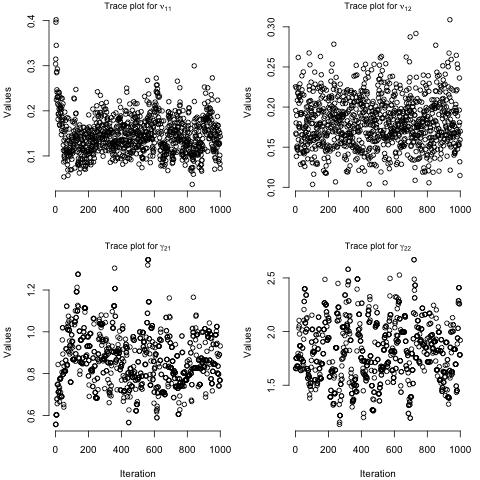
(a) Traceplots for Gibbs sampler

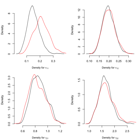
(b) Approximate posterior density

Figure 1: MCMC traceplots and densities for simulation example

Beyond posterior distributions for parameters, one is typically interested in posterior distributions of the survival functions. Note, there are two distinct sources of variation – (1) intermittent observations and (2) parameter uncertainty. The MCMC sampling procedure accounts for both, allowing for survival functions to be constructed for each iteration of the MCMC sampler using each iterations’ latent process and parameters. Figure 2 presents the pointwise median, $5$%, and $95$% survival at every time since recruitment when the individual is healthy and ill at baseline respectively. The red curves are the true survival function given healthy/ill at baseline. We see that the posteriors for survival functions are almost exactly equal, suggesting intermittent observations did not significantly impact our ability to predict survival of future patients.

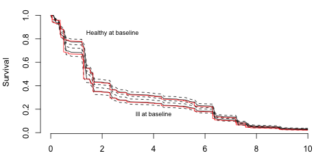
Figure 2: Survival functions given baseline state; median (black), 5% and 95% quantiles (dotted black), and true survival function (red)

9 A worked example: Cardiac allograft vasculopathy (CAV) data

To illustrate our methodology, we use data from angiographic examinations of 622 heart transplant recipients at Patworth Hopsital in the United Kingdom. This data was downloaded from the R library http://cran.r-project.org/web/packages/msm maintained by Christopher Jackson. Cardiac allograft vasculopathy (CAV) is a deterioration of the arterial walls. Four states were defined for heart transplant recipients: no CAV $(s=1)$, mild/moderate CAV $(s=2)$, severe CAV $(s=3)$, and dead $(s=4)$. The transition graph is given by Figure 3. Yearly examinations occurred for up to 18 years following the transplant. Mean follow-up time, however, is $5.9$ years. Survival times are observed and/or censored, but CAV state was only observed at appointment times prior to death/censoring. For censored recovrds, the censoring time is assumed to be the final appointment time. Out of the $622$ patients, Only $192$ patients were observed in state $2$ (Mild CAV) at any point during their follow-up. Out of these $192$, $43$ of these patients were subsequently observed in state $1$. Only $92$ patients were observed in state $3$ (Severe CAV) at any point during their follow-up. Out of these $92$, $12$ of these patients were subsequently observed in state $2$. There was no overlap in the these two patient subsets.

We set $B=(\{1,2,3\},\{4\})$, and assume the underlying process is a $B$-composable, exchangeable, Markov multi-state survival process. Parameters are $\{\rho_{(j,j^{\prime})},\lambda_{(j,j^{\prime})}\}_{j,j^{\prime}=1,2}$, $\{\gamma_{l,1},\gamma_{l,2}\}_{l\in B_{1}}$, and $\alpha_{2,1}\in[0,1]$. For identifiability, we set $\gamma_{1,1}$ and $\gamma_{1,2}$ equal to one. As transitions from state $2$ to $1$ occur but should not occur too often, the prior on $\alpha=\alpha_{2,1}$ is set to a Beta distribution with parameters $2$ and $8$ respectively. For parameters $\nu_{11}$ and $\nu_{12}$, the Gamma prior has hyperparameters $1$ and $1$. Parameters $(\gamma_{21},\gamma_{22},\gamma_{31},\gamma_{32})$ have independent, standard log-normal priors. We use the approximate MCMC sampler to perform inference.

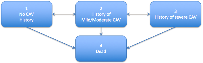
Figure 3: Cardiac allograft vasculopathy (CAV) transition diagram.

Traceplots in Figure 4(a) suggest convergence after the first 100 iterations. The MCMC sampler gives posteriors for the parameters. The posterior mean of $\nu_{11}$ is $0.75$ (i.e., marginal time until transition from state $1$ to state $2$ is $1.33$ years). Parameters $(\gamma_{21},\gamma_{31})$ have posterior means $(2.43,0.65)$, translating into marginal holding times of $0.59$ and $2.02$ years respectively. The posterior mean for $\alpha$ is $0.38$, suggesting that the patient is a bit more likely to experience progression of the CAV status than regression. The posterior mean for $\nu_{12}$ is $0.52$ (i.e., marginally the holding time in state $1$ until a transition to state $4$ is $1.92$ years). This suggests that in state $1$, disease progression is slightly more likely than failure. Parameters $(\gamma_{22},\gamma_{32})$ have posterior means $(1.10,1.81)$ respectively. This translates marginally into holding times of $1.76$ and $1.10$ years respectively. For state $2$, the distribution of $\gamma_{22}$ does overlap $1.0$ suggesting that failure transitions from states $1$ and $2$ may occur at similar rates.

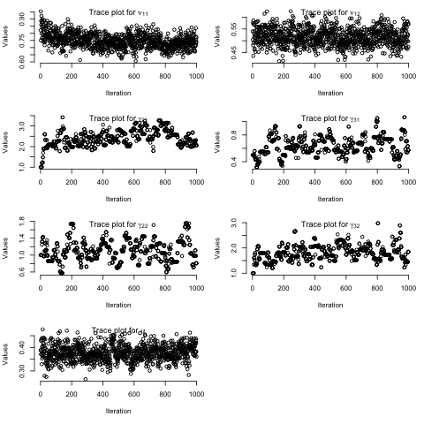
(a) Traceplots for MCMC algorithm

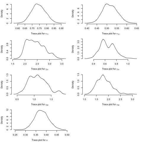
(b) Approximate posterior densities

Figure 4: MCMC traceplots and densities for CAV study

We next consider the posterior distributions for the survival functions. Figure 5(a) plots median survival at each time $t$ over all iterations of the MCMC sampler as well as the Kaplan-Meier survival function estimator. Note at baseline, all patients are in state $1$; therefore, the Kaplan-Meier curve should be compared with the median survival curve given the new patient is in state $1$. We see that the posterior survival curve is significantly lower. This reflects expected disease progression since baseline; that is, a new patient in state $1$ at baseline who is alive at time $t$ is likely to have seen a progression in their disease state, leading to an increase in their current risk of failure. Under the multi-state survival process model, the expected survival time from baseline given new patient is in state $1$, $2$, and $3$ is $8.75$, $8.32$, and $7.32$ respectively. Under the Kaplan-Meier estimator, the expected survival time from baseline is $9.66$. We have included the 5% and 95% quantiles for the survival function at each time $t$ when the patient is in state $3$ at baseline. Figure 5(b) plots median survival over all iterations of the MCMC sampler given the user is alive at time $t=5$. Under the multi-state survival process model, the expected survival time from time $5$ given new patient is in state $1$, $2$, and $3$ is $5.97$, $5.55$, and $5.04$ respectively. We again include the 5% and 95% quantiles for the survival function at each time $t$ when the patient is in state $3$ at baseline.

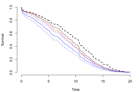
(a) Survival functions at baseline

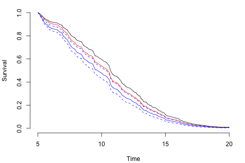
(b) Survival functions at $t=5$

Figure 5: Survival functions given “No CAV” (black), “Mild/Moderate CAV” (red), and “Severe CAV” (blue); Kaplan-Meier estimator (dotted black).

10 Concluding remarks

The preceding pages lay a theoretical and methodological foundation for the development of exchangeable, Markov multi-state survival processes. The approach put forward sits between the prior parametric and non-parametric approaches for multi-state survival data. A representation theorem characterizes the entire space of exchangeable, Markov multi-state processes via a measure $\Sigma$ and constants ${\bf c}$. Restrictions on choice of measure were driven by prior work on weak continuity and the notion of composable systems developed in this paper. To fit the models to intermittently observed multi-state survival data, extensions of existing MCMC samplers for Markov jump processes were required; an approximate MCMC sampler version was derived that achieved good empirical performance in simulations and led to significant decreases in runtime. Application to cardiac allograft vasculopathy (CAV) data showed how to interpret posterior parameter distributions. Comparison to Kaplan-Meier estimators showed how the model adjusts the non-parametric survival function estimator to account for disease progression.

Appendix A Proof of discrete-time characterization

We start with a discussion of an equivalent matrix representation used in proofs of both discrete and continuous-time characterizations.

A.1 Matrix equivalent representation

For every $y\in[s]^{\mathbb{N}}$, there exists an equivalent representation as a matrix with an infinite number of rows and $k$ columns $M\in[s]^{\mathbb{N}\otimes k}$ where the first row $M_{1,\cdot}=[y_{1},\ldots,y_{k}]$. Let $M_{\cdot,i}\in[s]^{\mathbb{N}}$ denote the $i$th column of $M$ (i.e., $M=[M_{\cdot,1}\,|\,\ldots\,|\,M_{\cdot,k}]$. Exchangeability of ${\bf Y}$ implies column exchangeability of ${\bf M}$. That is, for a set of permutations $(\sigma_{1},\ldots,\sigma_{k})$ such that $\sigma_{i}:\mathbb{N}\to\mathbb{N}$ for $i=1,\ldots,k$, we have

$${\bf M}=[{\bf M}_{\cdot,1}\,|\,\ldots\,|\,{\bf M}_{\cdot,k}]\overset{D}{=}[{\bf M}_{\cdot,1}^{\sigma_{1}}\,|\,\ldots|\,{\bf M}^{\sigma_{k}}_{\cdot,k}]={\bf M}^{\sigma}$$

where $\overset{D}{=}$ stands for equivalent in distribution. We define this property as column-wise exchangeable. Note exchangeability implies column-wise exchangeability but not vice versa. Restriction acts column-wise

$${\bf M}^{[n]}=[{\bf M}^{[n]}_{\cdot,1}\,|\,\ldots\,|\,{\bf M}_{\cdot,k}^{[n]}]$$

with such matrices in one-to-one correspondence with elements in $[s]^{[n\cdot k]}$.

We define an action of the matrix representation $A$ on $y\in[s]^{\mathbb{N}}$ by $A(y)=(A_{1,y_{1}},A_{2,y_{2}},\ldots)$. In other words, the $i$th row of $A$, $A_{i,\cdot}$, acts on $y_{i}$ by sending it to $A_{i,y_{i}}$. The identity map $I$ is defined by each row $I_{i,\cdot}$ being equal to $[12\ldots k]$; then $I(y)=y$ for all $y\in[s]^{\mathbb{N}}$. The equivalent vector representation of $I$ is defined as $\text{id}\in[s]^{\mathbb{N}}$.

We express the asymptotic frequency of $A$ by $k$-vector $|A|_{k}=(|A_{1}|,\ldots,|A_{k}|)$ assuming $|A_{i}|$ exists.

The proofs below are for the complete graph case. As $G$ is simply a restriction of the measure to a particular subset of transition matrices $\mathcal{P}_{G}$, the proofs below yield the desired results.

Proof of Theorem 1.

By Kolmogorov consistency, ${\bf Y}_{[n]}$ is a Markov chain governed by transition probability rules $\text{pr}({\bf Y}(t)=y^{\prime}\,|\,{\bf Y}(t-1)=y)$. Restriction to $[n]$ yields a transition rule for $y,y^{\prime}\in[s]^{[n]}$:

$$\text{pr}_{n}({\bf Y}_{[n]}(t)=y^{\prime}\,|\,{\bf Y}_{[n]}(t-1)=y)=\text{pr}({\bf Y}(t)=R_{n}^{-1}(y^{\prime})\,|\,{\bf Y}(t-1)=y^{\star})$$

where $R_{n}$ is the restriction operation so $R_{n}^{-1}(y^{\prime})=\{y\in[s]^{\mathbb{N}}\text{ s.t. }R_{n}(y)=y^{\prime}\}$ and $y^{\star}\in R_{n}^{-1}(y)$. Without loss of generality, we focus on time $t=1$.

We define a measure $\eta$ by

$$\eta(\cdot):=\text{pr}(\cdot\,|\,\text{id})$$

Via the matrix representation, we can think of $\eta$ as a measure on matrices $A\in[s]^{\mathbb{N}\otimes k}$. Restriction to $[n]$ yields $A^{[n]}\sim\eta^{[n]}(\cdot)=\text{pr}_{nk}(\cdot\,|\,\text{id}_{nk})$. The action of $A^{[n]}$ on $x\in[s]^{[n]}$ is then given by

$$A^{[n]}(x)=\eta^{[n]}(x)=\text{pr}_{n}(\cdot\,|\,I_{n}(x))=\text{pr}_{n}(\cdot\,|\,x)$$

as we require.

The above argument shows that there exists a measure $\eta$ such that ${\bf Y}^{\star}$ defined by

$${\bf Y}^{\star}(t)=(A_{t}\circ A_{t-1}\circ\ldots A_{1})(Y_{0}^{\star})$$

is equivalent in distribution to ${\bf Y}$. Here $A_{t}$ are independent, identical distributed draws from $\eta$ for each time $t\in\mathbb{N}$.

∎

Proof of Corollary 2.

Consider the recurrent event process ${\bf Y}$ up time $\tau<\infty$. Then ${\bf Y}^{\star}=\tau\wedge{\bf Y}$ is a version of ${\bf Y}$ on $t\in 0,1,\ldots,\tau$. Let $\eta_{\tau}$ to denote the measure associated with ${\bf Y}^{\star}$. For $P\in\mathcal{P}_{\tau}$, let $R_{\tau^{\prime},\tau}(A)$ be the restriction of this $\mathcal{P}_{\tau^{\prime}}$. Then for $\tau^{\prime}<\tau$

$$\eta_{\tau}(\{P\in\mathcal{P}_{\tau}\,|\,R_{\tau^{\prime},\tau}(P)=P^{\star}\})=\eta_{\tau^{\prime}}(\{P^{\star}\})$$

So we have consistency across $\tau>0$. We define the measure $\eta$ on $\mathcal{P}_{\infty}$ by

$$\eta(\cdot)=\lim_{\tau\uparrow\infty}\eta_{\tau}(\cdot)$$

is the unique measure such that ${\bf Y}^{\star}$ is a version of ${\bf Y}$. ∎

Appendix B Proof of continuous-time characterization

Again the proof below is for the complete graph case. As $G$ is simply a restriction of the measure to a particular subset of transition matrices $\mathcal{P}_{G}$, the proof below yields the desired result.

Proof of Theorem 2.

Like in the discrete-case, we construct the measure $\eta$ from the transition rule which governs ${\bf Y}$. This will connect ${\bf Y}^{\star}$ to ${\bf Y}$ such that they are equal in law.

Since ${\bf Y}_{[n]}$ is a Markov process on $[s]^{[n]}$, it is governed by a transition rate function

$$Q_{n}(y,y^{\prime})=\lim_{t\downarrow 0}\frac{1}{t}\text{pr}({\bf Y}_{[n]}(t)=y^{\prime}\,|\,{\bf Y}_{[n]}(0)=y).$$

We start by describing the key characteristics of the transition rate function

1. The transition rate function exhibits finite activity:

   $$\sum_{y^{\prime}\neq y}Q_{n}(y,y^{\prime})<\infty$$

2. The transition rate function is exchangeable. That is, for any $\sigma:\mathbb{N}\to\mathbb{N}$ and $y\neq y^{\prime}$:

   $$Q_{n}(y,y^{\prime})=Q_{n}(y^{\sigma},(y^{\prime})^{\sigma}).$$

3. The transition rate functions are consistent. That is, for $y,y^{\prime}\in[s]^{[m]}$ and $m\leq n$,

   $$Q_{m}(y,y^{\prime})=Q_{n}(y^{\star},R_{m,n}^{-1}(y^{\prime}))$$

   where $R_{m,n}^{-1}$ is the inverse of the restriction operator from $[n]$ to $[m]$ and $y^{\star}\in R_{m,n}^{-1}(y)$.

We then define the measure for $A\in[s]^{[n]\times s}\backslash\{\text{id}_{k,n}\}$ as

$$\eta_{n}(A)=Q_{n}(\text{id}_{k,n},A)$$

This measure is is column-wise exchangeable by exchangeability of $Q$ and satistfies

$$\eta_{n}(A)=\eta\left(\{A^{\star}:[s]^{[n]\times s}\,|\,(A^{\star})^{[n]}=A\}\right)$$ (10)

for all $m\leq n$ and $A\in[s]^{\mathbb{N}\times s}$ by consistency of $Q$.

The measure $\eta(A)=Q_{n}(\text{id}_{k},A)$ is also column-wise exchangeable and satisfies

• $\eta(\{\text{id}_{k}\})=0$ (i.e., a transition must occur) and

• $\eta(\{A\,|\,A^{[n]}\neq\text{id}_{k,n})<\infty$ (i.e., finite, restricted activity)

Following Pitman [2003], we construct a process ${\bf Y}^{\star}=({\bf Y}^{\star}(t),t\geq 0)$ via its finite restrictions ${\bf Y}_{[n]}^{\star}=({\bf Y}_{[n]}^{\star}(t),t\geq 0)$. Let ${\bf A}=\{(t,A)\subset\mathbb{R}^{+}\times[s]^{\mathbb{N}\otimes k}\}$ be a Poisson point process with intensity $dt\otimes\eta$. Given an inital state ${\bf Y}^{\star}(0)$, for each $t>0$ if $t$ is an atom of ${\bf A}$ then

• if $A_{t}^{[n]}\neq\text{id}_{k,n}$, then set ${\bf Y}_{[n]}^{\star}(t)=A_{t}^{[n]}({\bf Y}_{[n]}^{\star}(t-))$

• otherwise ${\bf Y}_{[n]}^{\star}(t)={\bf Y}_{[n]}^{\star}(t-)$

The difference between the continuous and discrete-time setting is the random time between jumps and that the jumps (1) occur for an infinite fraction of the units as $n\to\infty$, or (2) occur for a single unit $u\in\mathbb{N}$. By construction for $m\geq n$, the restriction of $Y_{[m]}^{\star}$ to $[n]$ is consistent with $Y_{[n]}^{\star}$ so we have ${\bf Y}^{\star}$ is a unique $[s]^{\mathbb{N}}$-valued process.

Lemma 1.

The process ${\bf Y}^{\star}$ is a Markov, exchangeable state-space process.

Proof.

Consistency is given by the above argument; the process is Markovian by construction and the assumptions on ${\bf Y}$. Exchangeability is due to $\eta$ being a column-wise exchangeable measure since $\eta_{[n]}$ are finite, column-wise exchangeable measures. ∎

The final concern before showing that ${\bf Y}^{\star}$ is stochastically equivalent to ${\bf Y}$ is the uniqueness of the measure $\eta$ related to the restricted measures $\eta_{n}$.

Lemma 2.

There exists unique measure $\eta$ on $[s]^{\mathbb{N}\otimes s}$ which satisfies (1) $\eta(\{\text{id}_{k}\})=0$, (2) $\eta(\{A\in[s]^{\mathbb{N}\otimes s}\,|\,A^{[n]}\neq\text{id}_{k,n}\})<\infty$, and

$$\eta(\{A^{\star}\in[s]^{\mathbb{N}\otimes s}\,|\,(A^{\star})^{[n]}=A\})=\eta_{n}(A)$$ (11)

for all $n>0$ and $A\in[s]^{[n]\otimes s}$.

Proof.

The sets

$$\{A^{\star}\in[s]^{\mathbb{N}\otimes s}\,|\,(A^{\star})^{[n]}=A\}$$

are a $\pi$-system generating the $\sigma$-field on $[s]^{\mathbb{N}\otimes s}$. The above discussion proves equation 11; and the measure is additive. Therefore, uniqueness is a consequence of any measure extended to a $\sigma$-algebra being unique if the measure is $\sigma$-finite. ∎

Lemma 3.

${\bf Y}^{\star}$ is a version of ${\bf Y}$.

Proof.

First, the finite restrictions $\eta_{n}$ satisfies

$$\eta_{n}(\{A\in[s]^{[n]\otimes s}\,|\,A(y)=y^{\prime}\}) =\sum_{A:A(y)=y^{\prime}}Q_{nk}(I_{k,n},A)$$

$$=Q_{n}(I_{k,n}(y),A(y))=Q_{n}(y,y^{\prime}).$$

And has finite activity:

$$\eta_{n}(\{A\in[s]^{[n]\otimes s}\,|\,A(y)=y\})=\sum_{y^{\prime}\neq y}Q_{n}(y,y^{\prime})<\infty$$

Therefore $({\bf Y}^{\star})^{[n]}$ is an Markov, exchangeable process with jump rates $Q_{n}(\cdot,\cdot)$. By Kolmogorov’s extension theorem, the unique process ${\bf Y}^{\star}$ is a version ${\bf Y}$. ∎

We still need to show $\eta$ can be decomposed into the respective components:

• Dislocation measure: measure on $s\times s$ transition matrices$\sim\Sigma$ which satisfies

  $$\Sigma(\{I_{k}\}) =0$$

  $$\int_{\mathcal{P}_{k}}(1-P_{\min})\Sigma(dP) <\infty$$

  where $P_{\min}=\min_{i}P_{i,i}$.

• Erosion measures: Let $A\in[s]^{\mathbb{N}\times s}$ then we call this $A=\text{id}$ and we flip a single unite $u\in\mathbb{N}$ (i.e., $A_{u,i}=i^{\prime}$). Let $\mu^{u}_{i,i^{\prime}}$ be this point mass measure. Define

  $$\mu_{i,i^{\prime}}=\sum_{u\in\mathbb{N}}\mu^{u}_{i,i^{\prime}}$$

• The combined measure is given by:

  $$\eta_{\Sigma,c}(\cdot)=\mu_{\Sigma}(\cdot)+\sum_{i\neq i^{\prime}\in[s]}c_{ii^{\prime}}\mu_{i,i^{\prime}}(\cdot)$$

Lemma 4.

The measure $\eta_{\Sigma,c}$ is a column-wise exchangeable measure satisfying the necessary constraints.

Proof.

We prove this for each component of $\eta_{\Sigma,c}$. First, $\mu_{\Sigma}(\{\text{id}_{k}\})=0$ by construction. Moreover, for $P\in\mathcal{P}_{k}$

$$\mu_{P}(\{A\,|\,A^{[n]}\neq\text{id}_{s,n}\}) \leq\mu_{P}(\{A\,|\,A^{[n]}\neq\text{id}_{s,n})$$

$$\leq\sum_{j=1}^{s}\mu_{P}(\{A\,|\,A^{[n]}_{u,j}\neq j\text{for all }u\in[n]\})$$

$$\leq k(1-p_{\min}^{n})\leq n\cdot k(1-p_{\min}^{n})$$

which implies

$$\mu_{\Sigma}(\{A\,|\,A^{[n]}\neq\text{id}_{s,n}\})\leq n\cdot k\int_{\mathcal{P}_{k}}(1-p_{\min})\Sigma(dP)<\infty$$

by the above assumptions.

Second, $\mu_{i,i^{\prime}}(\{\text{id}_{k}\})=0$ by construction. Moreover,

$$\sum_{i\neq i^{\prime}\in[s]}c_{ii^{\prime}}\mu_{i,i^{\prime}}(\{A\,|\,A^{[n]}\neq\text{id}_{s,n}\}) \leq c_{\max}\sum_{i\neq i^{\prime}\in[s]}\sum_{u\in[n]}\mu^{u}_{i,i^{\prime}}(\{A\,|\,A^{[n]}\neq\text{id}_{s,n}\})$$

$$\leq c_{\max}{s\choose 2}n<\infty.$$

∎

So we have that ${\bf Y}^{\star}$ is a version of ${\bf Y}$ and for any $\Sigma$ and $c$ the measure is $\mu_{\Sigma,c}$ is column-wise exchangeable satisfying necessary constraints. It rests to connect show that the measure $\eta$ can be decomposed such that there exists $\Sigma$ and $c$ such that $\eta=\mu_{\Sigma,c}$.

Lemma 5.

For $\eta$ constructed from $Q$, $\eta$-almost every $A\in[s]^{\mathbb{N}\otimes s}$ possesses asymptotic frequencies $|A|_{s}\in\mathcal{P}_{s}$.

Proof.

The $\eta$ by construction satisfies the necessary conditions. We set $\eta_{n}=\eta$ on $\{A\,|\,A^{[n]}\neq\text{id}_{s,n}\}$. Then $\eta_{n}$ is column-wise exchangeable for $(\sigma_{1},\ldots,\sigma_{s})$ such that $\sigma_{i}:\mathbb{N}\to\mathbb{N}$ fixes $[n]$.

We can find a column-wise exchangeable measure by simply considering ignoring the first $n$ rows. Let $\eta_{n}^{\prime}$ be measure obtained from $\eta$ after applying the $n$-shift function $\phi_{n}:A\to A^{\prime}$. Then $\eta_{n}^{\phi}$ is column-wise exchangeable and therefore has asymptotic frequencies. But asymptotic frequencies only depend on such an $n$-shift for every fixed $n>0$ (i.e., $|A|_{s}=|\phi_{n}(A)|_{s}$); therefore, $\eta_{n}$-almost every $A$ has asymptotic frequencies.

To prove $\eta$-almost every $A$ has asymptotic frequencies we simply note that $\eta_{n}\uparrow\eta$ and therefore the monotone convergence theorem completes proof. ∎

Lemma 6.

There exists a measure $\Sigma$ such that the restriction of $\eta$ to $\{|A|_{s}\neq I_{s}\}$ is equivalent to $\mu_{\Sigma}$.

Proof.

Let $\phi_{n}(A)^{[m]}$ denote the restriction of $\phi_{n}(A)$ to $[m]$. Then

$$\eta_{n}(\{\phi_{n}(A)^{[2]}\neq\text{id}_{s,2}\}\,|\,|A|_{s}=P) =\eta^{\phi}_{n}(\{\phi_{n}(A)^{[2]}\neq\text{id}_{s,2}\}\,|\,|A|_{s}=P)$$

$$=\eta^{\phi}_{n}(\{A^{[2]}\neq\text{id}_{s,2}\}\,|\,|A|_{s}=P)$$

$$=\mu_{P}(\{A^{[2]}\neq\text{id}_{s,2}\})$$

$$\geq 1-p_{\min}^{2}\geq 1-p$$

$$\Rightarrow\eta_{n}(\{A^{[2]}\neq\text{id}_{s,2}\}) \geq\int_{\mathcal{P}_{k}}(1-p_{\min})\Sigma_{n}(dP)$$

with $\Sigma_{n}=\eta_{n}{\bf 1}[|A|_{k}\neq I_{k}]$. As $n\to\infty$ this yields,

$$\infty>\eta(\{\phi(A)^{[2]}\neq\text{id}_{s,2}\})\geq\int_{\mathcal{P}_{s}}(1-p_{\min})\Sigma(dP)$$

and $\Sigma(\{\text{id}_{s}\})=0$ by construction.

It rests to show that $\mu_{\Sigma}={\bf 1}[|A|_{s}\neq\text{id}_{s}]\eta$. We have

$$\eta(\{A^{[n]}=A^{\star},|A|_{s}\neq\text{id}_{s}\})=\lim_{m\uparrow\infty}\eta_{m}(\{A^{[n]}=A^{\star},A^{[m]}\neq\text{id}_{s,m},|A|_{s}\neq\text{id}_{s}\})$$

The right hand side is equivalent to

$$\eta^{\phi}_{m}(\{A^{[n]}=A^{\star},|A|_{s}\neq\text{id}_{s}\}) =\int_{\mathcal{P}_{s}}\mu_{P}(\{A^{[n]}=A^{\star}\})|\eta_{m}^{\phi}|(|A|_{s}\in dP)$$

$$=\int_{\mathcal{P}_{k}}\mu_{P}(\{A^{[n]}=A^{\star}\})\Sigma(dP)$$

$$=\mu_{\Sigma}(\{A^{[n]}=A^{\star}\})$$

∎

Lemma 7.

There exists a set of constants $\{c_{i,i^{\prime}}\}_{i\neq i^{\prime}\in[s]}$ such that the restriction of $\eta$ to $\{|A|_{s}=I_{s}\}$ is equivalent to $\mu_{c}(\cdot)=\sum_{i\neq i^{\prime}\in[s]}c_{ii^{\prime}}\mu_{i,i^{\prime}}(\cdot)$.

Proof.

We restrict our attention to the set of $A$ where $A^{[2]}\neq\text{id}_{s,2}$ but $\phi_{3}(A)=\text{id}_{s}$. This set $B$ contains all single unit transition. As the measure $\eta_{3}^{\phi}$ is proportional to the point mass at $\text{id}_{s}$, then $\eta$ restricted to the event $\{A^{[2]}\neq\text{id}_{s,2},\phi_{3}(A)=\text{id}_{s},|A|_{s}=\text{id}_{s}\}$ is the sum

$$\sum_{A\in B}c_{A}\delta_{A}(\cdot).$$

If $A$ contains more than a single unit transition, exchangeability forces $c_{A}=0$ since $\eta(\{A\,|\,A^{[2]}\neq\text{id}_{s,2}\})<\infty$. The same argument shows $A\in[s]^{\mathbb{N}\otimes s}$ such that $|A|_{s}=I_{s}$ and $c_{A}>0$ implies $A$ is a single unit transition. ∎

This concludes the proof.

∎

Appendix C Examples

Here, we describe several important examples that motivate the current study of multi-state survival processes.

Example 1 (Survival process).

A survival process has state space { Alive, Dead } with transitions governed by the simple graph shown in Figure 6. In this case, $s=2$ and the edge-set is the singleton $\{(1,2)\}$; because the state “Dead” is absorbing, the space $\mathcal{P}_{G}$ is equivalent to the one-dimensional space $p\in[0,1)$. Restricting to $[n]$, suppose that all individuals at time $t$ are still at risk. In discrete-time, the probability of $d$ individuals passing away between times $t$ and $t+1$ is equal to

$$\int_{0}^{1}p^{n-d}(1-p)^{d}\Sigma(dp)$$

where $\Sigma$ is a probability measure on $(0,1]$. The marginal distribution of the survival time for each patient is geometric. Letting $\Sigma(dp)$ be the conjugate prior $\nu\cdot p^{\alpha-1}(1-p)^{\beta-1}dp$ with $\alpha,\beta>0$ yields a discrete-version of the “beta-splitting” process [Aldous, 1996]. The marginal geometric distribution in this case has parameter $\beta/(\alpha+\beta)$.

Figure 6: Graph representation of survival process

In continuous-time, the probability of $d$ individuals passing away between times $t$ and $t+1$ is proportional to

$$\int_{0}^{1}p^{n-d}(1-p)^{d}\Sigma(dp)+\delta(d=1)c_{1,2}$$

where $\Sigma$ is a measure on $(0,1]$ satisfying $\int(1-p)\Sigma(dp)<\infty$. In continuous-time, the marginal distribution is exponential. The conjugate prior now relaxes the constraints to $\beta>-1$. Considering choice of measure, Dempsey and McCullagh 2017 suggest choosing measure with $\beta=0$ – called the harmonic process. The harmonic process is the only family of Markov survival processes with weakly continuous predictive distributions – a key property in applied work. The chance of singleton events is set to zero (i.e., $c_{1,2}=0$).

Example 2 (Illness-death process).

The illness-death process has state space { Healthy, Unhealthy, Dead} with transitions governed by the simple graph shown in Figure 7. The state “Dead” (i.e., $s=3$) is absorbing, the space $\mathcal{P}_{G}$ is equivalent to a three-dimensional space. The bi-directional illness-death process includes the additional edge (Unhealthy,Health), allowing the patient to recover. Both processes can be viewed as refinements of the survival process.

Figure 7: Graph representation of the illness-death process

An issue arises for the bi-directional illness-death process when the definitions of “Healthy” and “Unhealthy” are arbitrary (i.e., have no scientific value). Potentially the labels are exchangeable and, if so, the process is a Markov exchangeable survival process. Such considerations lead to natural constraints on the choice of measure – see section 6 for a discussion.

Example 3 (Comorbidities).

Comorbidities are multiple stochastic processes experienced simultaneously by the same patient. Figure 8, for example, represents $L$ binary risk processes each with an absorbing state. In general, $Y(i,t)=(Y_{1}(i,t),\ldots,Y_{L}(i,t))$ is an $L$-vector state-space process.

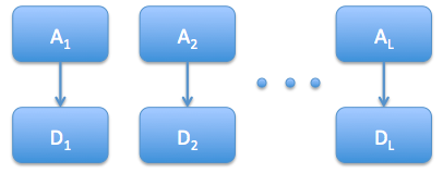
Figure 8: Graph representation of co-morbidities process

An example of comorbidities is provided by Aalen et al. [1980] where two events (onset of menopause, and occurrence of chronic skin disease) were studied. Patients could also experience a third event, death. In this case, we have $L=2$ binary risk processes each with absorbing states and then a final absorbing state of death.

Example 4 (Competing risks).

A patient may experience failure for a multitude of reasons. Figure 9 shows a setting where failure can be caused by $L$ risks. Unlike comorbidities, a patient may only experience one of the competing risks.

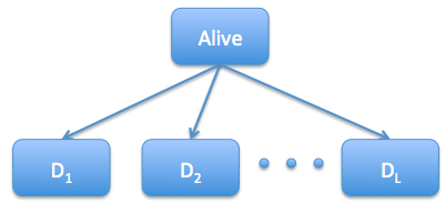
Figure 9: Graph representation of competing risks process

Example 5 (Recurrent events).

Recurrent events are events that occur more than once per patient. Examples include recurring hospital admissions, tumor recurrence, and repeated heart attacks. For recurrent events, the state-space is countably infinite; however, the state-space is structured. We can assume all patients initial values are zero (i.e. $Y(u,0)=0$) and given $Y(u,t)=k$ then the transition at the next jump time must be to $k+1$. This structure allows us to provide the following discrete and continuous-time characterizations of the exchangeable, Markov recurrent event processes – extending Theorems 1 and 2.

Corollary 2 (Discrete-time characterization).

Let ${\bf Y}=({\bf Y}(t),t\in\mathbb{N})$ be a discrete-time Markov, exchangeable recurrent event process. Then there exists a probability measure $\Sigma$ on $[0,1]^{\mathbb{N}}$ such that ${\bf Y}_{\Sigma}^{\star}$ is a version of ${\bf Y}$.

Proof of Corollary 2.

Consider the recurrent event process ${\bf Y}$ up time $\tau<\infty$. Then ${\bf Y}^{\star}=\tau\wedge{\bf Y}$ is a version of ${\bf Y}$ on $t\in 0,1,\ldots,\tau$. Let $\eta_{\tau}$ to denote the measure associated with ${\bf Y}^{\star}$. For $P\in\mathcal{P}_{\tau}$, let $R_{\tau^{\prime},\tau}(A)$ be the restriction of this $\mathcal{P}_{\tau^{\prime}}$. Then for $\tau^{\prime}<\tau$

$$\eta_{\tau}(\{P\in\mathcal{P}_{\tau}\,|\,R_{\tau^{\prime},\tau}(P)=P^{\star}\})=\eta_{\tau^{\prime}}(\{P^{\star}\})$$

So we have consistency across $\tau>0$. We define the measure $\eta$ on $\mathcal{P}_{\infty}$ by

$$\eta(\cdot)=\lim_{\tau\uparrow\infty}\eta_{\tau}(\cdot)$$

is the unique measure such that ${\bf Y}^{\star}$ is a version of ${\bf Y}$. ∎

Corollary 3 (Continuous-time characterization).

Let ${\bf Y}=({\bf Y}(t),t\in\mathbb{R}^{+})$ be a continuous-time Markov, exchangeable recurrent event process such that ${\bf Y}_{u}(0)=0$ for all $u\in\mathbb{N}$. Let $I$ denote the infinite identity matrix. Then there exists a probability measure $\Sigma$ on $[0,1]^{\mathbb{N}}$ satisfying

$$\Sigma(\{I\})=0\text{ and }\int_{[0,1]^{\mathbb{N}}}(1-P_{\min})\Sigma(dp)<\infty\text{ where }P_{\min}=\min_{i\in\mathbb{N}}P_{i}$$

and a set of constants ${\bf c}=\{c_{i,i+1}\,|\,i\in\mathbb{N}\}$ such that ${\bf Y}_{\Sigma,c}^{\star}$ is a version of ${\bf Y}$.

A similar proof can be constructed for the continuous-time setting and is therefore omitted.

Appendix D Details on choice of measure

Let $Z$ be a positive, stationary Lévy process on $\mathbb{R}_{+}$. As these processes are positive, it is natural to work with the cumulant function

$$K(t)=\log\left(\mathbb{E}\left[e^{-Z(t)}\right]\right)=\log\left(\mathbb{E}\left[e^{-tX}\right]\right)$$

for $t\geq 1$ and $X=Z(1)$ is an infinitely divisible distribution. The Lévy-Khintchine characterization for positive, stationary, Lévy processes implies

$$K(t)=-\left[\gamma t+\int_{0}^{\infty}(1-e^{-ty})w(dy)\right]$$

for some $\gamma\geq 0$ and measure $w(\cdot)$ on $\mathbb{R}_{+}$, called the Lévy measure, such that the integral is finite for all $t>0$.

Dempsey and McCullagh [2017] showed that every exchangeable, Markov survival process can be generated via a Lévy process construction. The proof stems from connecting $\gamma$ to the erosion measures (i.e., $c\geq 0$ in Theorem (2)) and the Lévy measure to the dislocation measures (i.e., $\Sigma(\cdot)$ in Theorem (2)). For instance, the harmonic process can be constructed via a Lévy process with $\gamma=0$ and $w(dy)=\nu e^{-\rho y}dy/(1-e^{-y}))$.

Now consider the proportional conditional hazards model as described by Kalbfleisch [1978], Hjort [1990], and Clayton [1991]. In the proportional conditional hazards model, the hazard for individual $i$ is $w_{i}Z(t)$ for some $w_{i}>0$ typically $w_{i}=\exp(x_{i}^{\prime}\beta)$ depending on a set of baseline covariates $x_{i}$. Then the conditional survival density for particle $i$ is $\exp\left(-w_{i}\int_{0}^{t}Z(t)\right)\left(1-e^{-w_{i}Z(t)}\right)$. Assume there is a single covariate that is a factor with a finite number of levels (i.e., $x_{i}\in\{1,\ldots,k\}:=[k]$). Then $w_{i}=w_{x_{i}}$; that is, there are a finite set of weights. The joint marginal density can be derived in a similar way as before. Here, however, the non-normalized transition rules are

$$\lambda(R,D) =\mathbb{E}\left(e^{-Z(t)\sum_{i\in R}w_{x_{i}}}\prod_{i\in D}\left(1-e^{-w_{x_{i}}Z(t)}\right)\right)$$

$$=\mathbb{E}\left(\prod_{j=1}^{k}\left(\exp(-Z(t))^{w_{j}}\right)^{r_{j}}\left(1-\exp(-Z(t))^{w_{j}}\right)^{d_{j}}\right)$$

$$=\int_{0}^{1}\prod_{j=1}^{k}\left(p^{w_{j}}\right)^{r_{j}}\left(1-p^{w_{j}}\right)^{d_{j}}\Sigma(dp)$$

where $r_{j}=\#\{i\in R\text{ s.t. }X_{i}=j\}$, $d_{j}=\#\{i\in D\text{ s.t. }X_{i}=j\}$, and $\Sigma(\cdot)$ is the dislocation measure. The final equality is due to the connection between the Lévy measure and the dislocation measure. It is clear from above that the proportional conditional hazards model corresponds to a particular choice of the dislocation measure. Namely, the proportional conditional hazards model corresponds to $p_{i}\to p^{w_{x_{i}}}$. So on the $[0,1]$-scale, the model is conditionally proportional on the log-scale. That is, $\log(p_{i})=w_{x_{i}}\log(p)$. Alternative choices exist. For example, the model may be conditionally proportional on the logistic scale; that is, $\log\left(p_{i}/(1-p_{i})\right)=w_{x_{i}}\log\left(p/(1-p)\right)$. We do not pursue such alternatives in this paper.

References

- Aalen et al. (1980) O. Aalen, O. Borgan, R.D. Gill, and N. Keiding. Interaction between life history events: nonparametric analysi of prospective and retrospective data in the present of censoring. Scand. J. Statist., 7:161–171, 1980.
- Aalen et al. (2008) O. Aalen, O. Borgan, and H. Gjessing. Survival and Event History Analysis: A Process Point of View. Springer-Verlag New York, New York, NY, 1 edition, 2008.
- Aalen et al. (2015) O. Aalen, T. Pedersen, O. Borgan, R. Hoff, K. Roysland, and S. S. Dynamic path analysis – a useful tool to investigate mediation processes in clinical survival trials. Statistics in Medicine, 34(29):3866–3887, 2015.
- Aldous (1996) David Aldous. Probability Distributions on Cladograms, pages 1–18. Springer, 1996.
- Breto et al. (2009) C. Breto, , D. He, E. Ionides, and A.A. King. Time series analysis via mechanistic models. The Annals of Applied Statistics, 3(1):319–348, 2009.
- Clayton (1991) D.G. Clayton. A monte carlo method for bayesian inference in frailty models. Biometrics, 47:467–485, 1991.
- De Finetti (1972) B. De Finetti. Probability, Induction and Statistics. John Wiley & Sons Ltd, 1 edition, 1972.