Cosmological Constraints on Unstable Particles:
Numerical Bounds and Analytic Approximations

Abstract

Many extensions of the Standard Model predict large numbers of additional unstable particles whose decays in the early universe are tightly constrained by observational data. For example, the decays of such particles can alter the ratios of light-element abundances, give rise to distortions in the cosmic microwave background, alter the ionization history of the universe, and contribute to the diffuse photon flux. Constraints on new physics from such considerations are typically derived for a single unstable particle species with a single well-defined mass and characteristic lifetime. In this paper, by contrast, we investigate the cosmological constraints on theories involving entire ensembles of decaying particles — ensembles which span potentially broad ranges of masses and lifetimes. In addition to providing a detailed numerical analysis of these constraints, we also formulate a set of simple analytic approximations for these constraints which may be applied to generic ensembles of unstable particles which decay into electromagnetically-interacting final states. We then illustrate how these analytic approximations can be used to constrain a variety of toy scenarios for physics beyond the Standard Model. For ease of reference, we also compile our results in the form of a table which can be consulted independently of the rest of the paper. It is thus our hope that this work might serve as a useful reference for future model-builders concerned with cosmological constraints on decaying particles, regardless of the particular model under study.

I Introduction

Many proposals for physics beyond the Standard Model (SM) predict the existence of additional unstable particles. The decays of such particles can have a variety of observable consequences — especially if the final states into which these particles decay involve visible-sector particles. Indeed, electromagnetic or hadronic showers precipitated by unstable-particle decays within the recent cosmological past can alter the primordial abundances of light nuclei both during and after Big-Bang nucleosynthesis (BBN) KawasakiMoroi ; Sarkar:1995dd ; CyburtEllisUpdated ; CyburtEllisGravitino ; Kawasaki:2017bqm , give rise to spectral distortions in the cosmic microwave background (CMB) HuAndSilk ; HuAndSilk2 , alter the ionization history of the universe Adams:1998nr ; ChenKamionkowski ; SlatyerFinkbeiner ; Finkbeiner:2011dx ; SlatyerInjectionHistory , and give rise to characteristic features in the diffuse photon background. These considerations therefore place stringent constraints on models for new physics involving unstable particles.

Much previous work has focused on examining the cosmological consequences of a single particle species decaying in isolation, and the corresponding limits on the properties of such a particle species are now well established. Indeed, simple analytic approximations can be derived which accurately model the effects that the decays of such a particle can have on many of the relevant observables HuAndSilk ; CyburtEllisUpdated ; KhatriSunyaev . However, many theories for new physics involve not merely one or a few unstable particles, but rather a large — and potentially vast — number of such particles with a broad spectrum of masses, lifetimes, and cosmological abundances. For example, theories with additional spacetime dimensions give rise to infinite towers of Kaluza-Klein (KK) excitations for any field which propagates in the higher-dimensional bulk. Likewise, string theories generally predict large numbers of light moduli BanksModuliProblem1 ; deCarlosModuliProblem ; BanksModuliProblem2 or axion-like particles WittenStringAxion ; SvrcekAndWitten ; Axiverse . Collections of similar light fields also arise in supergravity theories SUGRAModuliProblem , as well as in other scenarios for new physics NNaturalness ; TimRaffaeleMatt . There even exist approaches to the dark-matter problem such as the Dynamical Dark Matter (DDM) framework DDM1 ; DDM2 which posit the existence of potentially vast ensembles of unstable dark-sector particles. It is therefore crucial to understand the cosmological consequences of entire ensembles of decaying particles in the early universe and, if possible, to formulate a corresponding set of analytic approximations which model the effects of these decays.

For a variety of reasons, assessing the effects of an entire ensemble of decaying particles with a broad range of masses, lifetimes, and cosmological abundances is not merely a matter of trivially generalizing the results obtained in the single-particle case. The decay of a given unstable particle amounts to an injection of additional electromagnetic radiation and/or other energetic particles into the evolution of the universe, and injection at different characteristic timescales during this evolution can have markedly different effects on the same observable. Moreover, since many of these observables evolve in time according to a complicated system of coupled equations, the effects of injection at any particular time $t_{\mathrm{inj}}$ depend in a non-trivial way on the entire injection history prior to $t_{\mathrm{inj}}$ through feedback effects.

In principle, the cosmological constraints on ensembles of decaying particles in the early universe can be evaluated numerically. Indeed, there are several publicly available codes ChlubaGreensFns1 ; SlatyerInjectionHistory ; PPPC4DMID which can readily be modified in order to assess the effects of an arbitrary additional injection history on the relevant observables. Computational methods can certainly yield useful results in any particular individual case. However, another complementary approach which can provide additional physical insight into the underlying dynamics involves the formulation of approximate analytic expressions for the relevant observables — expressions analogous to those which already exist for a single particle species decaying in isolation. Our aim in this paper is to derive such a set of analytic expressions — expressions which are applicable to generic theories involving large numbers of unstable particles, but which nevertheless provide accurate approximations for the relevant cosmological observables. Thus, our results can serve as a useful reference for future model-builders concerned with cosmological constraints on decaying particles, regardless of the particular model under study.

In this paper, we shall focus primarily on the case in which electromagnetic injection dominates — i.e., the case in which the energy liberated by the decays of these particles is released primarily in the form of photons, electrons, and positrons rather than hadrons. We also emphasize that the approximations we shall derive in this paper are not ad hoc in nature; in particular, they are not the results of empirical fits. Rather, as we shall see, they emerge organically from the underlying physics and thus carry direct information about the underlying processes involved.

This paper is organized as follows. In Sect. II, we begin by establishing the notation and conventions that we shall use throughout this paper. We also review the various scattering processes through which energetic photons injected by particle decay interact with other particles present in the radiation bath. In subsequent sections, we then turn our attention to entire ensembles of unstable particles, focusing on the electromagnetic injections arising from decays occurring after the BBN epoch. Each section is devoted to a different cosmological consideration arising from such injection, and in each case we ultimately obtain a simple, analytic approximation for the corresponding constraint. For example, in Sect. III we consider the constraints associated with the modification of the abundances of light nuclei after BBN, and in Sect. IV we consider limits on distortions of the CMB-photon spectrum. Likewise, in Sect. V we consider the constraints associated with the ionization history of the universe and its impact on the CMB, and in Sect. VI we consider the constraints associated with additional contributions from unstable-particle decays to the diffuse photon background. Ultimately, the results from these sections furnish us with the tools needed to constrain decaying ensembles of various types. This is then illustrated in Sect. VII, where we consider how our results may be applied to two classes of ensembles whose constituents exhibit different representative mass spectra. Finally, in Sect. VIII, we conclude with a discussion of our main results and avenues for future work. For future reference, we also provide (in Table 4) a summary/compilation of our main results.

II Electromagnetic Injection:  Overview and Classification of Relevant Processes

Our aim in this paper is to assess the cosmological constraints on an ensemble consisting of a potentially large number $N$ of unstable particle species $\chi_{i}$ with masses $m_{i}$ and decay widths $\Gamma_{i}$ (or, equivalently, lifetimes $\tau_{i}\equiv\Gamma_{i}^{-1}$), where the index $i=0,1,\ldots,N-1$ labels these particle species in order of increasing mass $m_{i}$. We shall characterize the cosmological abundance of each of the $\chi_{i}$ in terms of a quantity $\Omega_{i}$ which we call the “extrapolated abundance.” This quantity represents the abundance that the species $\chi_{i}$ would have had at present time, had it been absolutely stable. We shall assume that the total abundance $\Omega_{\mathrm{tot}}\equiv\sum_{i}\Omega_{i}$ of the ensemble is sufficiently small that the universe remains radiation-dominated until the time of matter-radiation equality $t_{\mathrm{MRE}}\approx 10^{12}$ s. Moreover, we shall focus on the regime in which $m_{i}\gtrsim 1$ GeV for all $\chi_{i}$ and all of the ensemble constituents are non-relativistic by end of the BBN epoch. Within this regime, as we shall discuss in further detail below, the spectrum of energetic photons produced by electromagnetic injection takes a characteristic form which to a very good approximation depends only on the overall energy density injected KawasakiMoroi . By contrast, for much lighter decaying particles, the form of the resulting photon spectrum can differ from this characteristic form as a result of the immediate decay products lacking sufficient energy to induce the production of $e^{+}e^{-}$ pairs by scattering off background photons PoulinSerpico1 ; PoulinSerpico2 . The cosmological constraints on a single electromagnetically-decaying particle species with a mass below $1$ GeV — investigated earlier to constrain neutrinos (see, e.g., Ref. Sarkar:1984tt ) — have recently been investigated in Refs. Hufnagel ; ForestellMorrisseyWhite .

The considerations which place the most stringent constraints on the ensemble depend on the values of $\Omega_{i}$ and $\tau_{i}$ for the individual ensemble constituents. For ensembles of particles with lifetimes in the range $1\mbox{~{}s}\lesssim\tau_{i}\lesssim t_{\mathrm{now}}$, where $t_{\mathrm{now}}$ denotes the present age of the universe, the dominant constraints are those related to the abundances of light elements, to spectral distortions of the CMB, and to the ionization history of the universe. The effect of electromagnetic injection on the corresponding observables is sensitive to the overall energy density injected and to the timescales over which that energy is injected, but not to the details of the decay kinematics or the particular channels through which the $\chi_{i}$ decay. Thus, in order to retain as much generality as possible in our analysis, we shall focus on ensembles for which all constituents with non-negligible $\Omega_{i}$ have lifetimes within this range; moreover, we shall refrain from specifying any particular decay channel for the $\chi_{i}$ when assessing the bounds on these ensembles due to these considerations. By contrast, the constraints on decaying ensembles that follow from limits on features in the diffuse photon background do depend on the particulars of the decay kinematics. Thus, when analyzing these constraints in Sect. VI, we not only present a general expression for the relevant observable — namely the contribution to the differential photon flux from the decaying ensemble — but also apply this result to a concrete example involving a particular decay topology.

Many of the constraints on electromagnetic injection are insensitive to the details of the decay kinematics because the injection of photons and other electromagnetically-interacting particles prior to CMB decoupling sets into motion a complicated chain of interactions which serve to redistribute the energies of these particles. In particular, the effects of electromagnetic injection on cosmological observables ultimately depend on the interplay between three broad classes of processes through which these photons interact with other particles in the background plasma. These are:

• Class I: Cascade and cooling processes which rapidly redistribute the energy of the injected photons. Processes in this class include $\gamma+\gamma_{\mathrm{BG}}\rightarrow e^{+}+e^{-}$ and $\gamma+\gamma_{\mathrm{BG}}\rightarrow\gamma+\gamma$, where $\gamma_{\mathrm{BG}}$ denotes a background photon, as well as inverse-Compton scattering and $e^{+}e^{-}$ pair production off nuclei. These processes occur on timescales far shorter than the timescales associated with other relevant processes, and thus may be considered to be effectively instantaneous. As we shall see, these processes serve to establish a non-thermal population of photons with a characteristic spectrum.

• Class II: Processes through which the non-thermal population of photons established by Class-I processes can have a direct effect on cosmological observables. These include the photoproduction and photodisintegration of light elements during or after BBN, as well as the photoionization of neutral hydrogen and helium after recombination.

• Class III: Processes which serve to bring the non-thermal population of photons established by Class-I processes into kinetic and/or thermal equilibrium with the radiation bath. Processes in this class include Compton scattering, bremsstrahlung, and $e^{+}e^{-}$ pair production off nuclei.

We emphasize that these classes are not necessarily mutually exclusive, and that certain processes play different roles during different cosmological epochs.

Any energy injected in the form of photons prior to last scattering is rapidly redistributed to lower energies due to the Class-I processes discussed above. The result is a non-thermal contribution to the photon spectrum at high energies with a normalization that depends on the total injected power and a generic shape which is essentially independent of the shape of the initial injection spectrum directly produced by $\chi_{i}$ decays. This “reprocessed” photon spectrum serves as a source of for Class-II processes — processes which include, for example, reactions that alter the abundances of light nuclei and scattering processes which contribute to the ionization of neutral hydrogen and helium after recombination. Since all information about the detailed shape of the initial injection spectrum from decays is effectively washed out by Class-I processes in establishing this reprocessed photon spectrum, the results of our analysis are largely independent of the kinematics of $\chi_{i}$ decay. This is ultimately why many of our results — including those pertaining to the alteration of light abundances after BBN, distortions in the CMB, and the ionization history of the universe — are likewise largely insensitive to the decay kinematics of the $\chi_{i}$.

The timescale over which injected photons can cause these alterations is controlled by the Class-III processes. Prior to CMB decoupling, these processes serve to “degrade” the reprocessed photon spectrum established by Class-I processes by bringing this non-thermal population of photons into kinetic or thermal equilibrium with the photons in the radiation bath. As this occurs, these Class-III interactions reduce the energies of the photons below the threshold for Class-II processes while also potentially altering the shape of the CMB-photon spectrum. These Class-III processes eventually freeze out as well, after which point any photons injected by particle decays simply contribute to the diffuse extra-galactic photon background.

III Impact on Light-Element Abundances

We begin our analysis of the cosmological constraints on ensembles of unstable particles by considering the effect that the decays of these particles have on the abundances of light nuclei generated during BBN.  We shall assume that these decays occur after BBN has concluded, i.e., after initial abundances for these nuclei are already established. We begin by reviewing the properties of the non-thermal photon spectrum which is established by the rapid reprocessing of injected photons from these decays by Class-I processes. We then review the corresponding constraints on a single unstable particle species CyburtEllisUpdated — constraints derived from a numerical analysis of the coupled system of Boltzmann equations which govern the evolution of these abundances. We then set the stage for our eventual analysis by deriving a set of analytic approximations for the above constraints and demonstrating that the results obtained from these approximations are in excellent agreement with the results of a full numerical computation within our regime of interest. Finally, we apply our analytic approximations in order to constrain scenarios involving an entire ensemble of multiple decaying particles exhibiting a range of masses and lifetimes.

III.1 Reprocessed Injection Spectrum

As discussed in Sect. II, the initial spectrum of photons injected at time $t_{\mathrm{inj}}$ is redistributed effectively instantaneously by Class-I processes. A detailed treatment of the Boltzmann equations governing these processes in a radiation-dominated epoch can be found, e.g., in Ref. KawasakiMoroi . For injection at times $t_{\mathrm{inj}}\lesssim 10^{12}$ s, the resulting reprocessed photon spectrum turns out to take a characteristic form which we may parametrize as follows:

$$\frac{dn_{\gamma}(E,t_{\mathrm{inj}})}{dEdt_{\mathrm{inj}}}~{}=~{}\frac{d\rho(t_{\mathrm{inj}})}{dt_{\mathrm{inj}}}K(E,t_{\mathrm{inj}})~{}.$$ (1)

The quantity $d\rho(t_{\mathrm{inj}})/dt_{\mathrm{inj}}$ appearing in this expression, which specifies the overall normalization of the contribution to the reprocessed photon spectrum, represents the energy density injected by particle decays during the infinitesimal time interval from $t_{\mathrm{inj}}$ to $t_{\mathrm{inj}}+dt_{\mathrm{inj}}$. The function $K(E,t_{\mathrm{inj}})$, on the other hand, specifies the shape of the spectrum as a function of the photon energy $E$. This function is normalized such that

$$\int_{0}^{\infty}K(E,t_{\mathrm{inj}})EdE~{}=~{}1~{}.$$ (2)

It can be shown that for any process that injects energy primarily through electromagnetic (rather than hadronic) channels, the function $K(E,t_{\mathrm{inj}})$ takes the universal form EllisGelmini ; ProtheroeBerezinsky ; KawasakiMoroi

$$K(E,t_{\mathrm{inj}})~{}=~{}\begin{cases}K_{0}(E_{X}/E)^{3/2}&E<E_{X}\\ K_{0}(E_{X}/E)^{2}&E_{X}<E<E_{C}{}{}{}\\ 0&E>E_{C}~{},\end{cases}\\$$ (3)

where $K_{0}$ is an overall normalization constant and where $E_{C}$ and $E_{X}$ are energy scales associated with specific Class-I processes whose interplay determines the shape of the reprocessed photon spectrum. The normalization convention in Eq. (2) implies that $K_{0}$ is given by

$$K_{0}~{}=~{}\frac{1}{E_{X}^{2}\big{[}2+\ln(E_{C}/E_{X})\big{]}}~{}.$$ (4)

Physically, the energy scales $E_{C}$ and $E_{X}$ appearing in Eq. (3) can be understood as follows. The scale $E_{C}$ represents the energy above which the photon spectrum is effectively extinguished by the pair-production process $\gamma+\gamma_{\mathrm{BG}}\rightarrow e^{+}+e^{-}$, in conjunction with interactions between the resulting electron and positron and other particles in the thermal bath. The energy scale $E_{X}$ represents the threshold above which $\gamma+\gamma_{\mathrm{BG}}\rightarrow\gamma+\gamma$ is the dominant process through which photons lose energy. By contrast, below this energy threshold, the dominant processes are Compton scattering and $e^{+}e^{-}$ pair-production off nuclei. Note that while the normalization of the reprocessed photon spectrum is set by $d\rho(t_{\mathrm{inj}})/dt_{\mathrm{inj}}$, the shape of this spectrum is entirely controlled by the temperature $T_{\mathrm{inj}}$ at injection. This temperature behaves like $T_{\mathrm{inj}}\propto t_{\mathrm{inj}}^{-1/2}$ in a radiation-dominated epoch. This implies that as $t_{\mathrm{inj}}$ increases, the value of $E_{C}$ also increases. This reflects the fact that the thermal bath is colder at later injection times, and thus an injected photon must be more energetic in order for the pair-production process $\gamma+\gamma_{\mathrm{BG}}\rightarrow e^{+}+e^{-}$ to be effective. Numerically, the values of $E_{C}$ and $E_{X}$ at a given injection time $t_{\mathrm{inj}}$ are estimated to be KawasakiMoroi ; CyburtEllisUpdated

$$E_{C} = \frac{m_{e}^{2}}{22T_{\mathrm{inj}}}\approx\big{(}103\,\,{\rm MeV}\big{)}\times\left(\frac{t_{\mathrm{inj}}}{10^{8}\,\rm s}\right)^{1/2}$$

$$E_{X} = \frac{m_{e}^{2}}{80T_{\mathrm{inj}}}\approx\big{(}28\,\,{\rm MeV}\big{)}\times\left(\frac{t_{\mathrm{inj}}}{10^{8}\,\rm s}\right)^{1/2}~{},~{}~{}$$ (5)

where $m_{e}$ is the electron mass and $T_{\mathrm{inj}}$ is the temperature of the thermal bath at $t_{\mathrm{inj}}$.

The reprocessed photon spectrum in Eq. (1) is the spectrum which effectively contributes to the photoproduction and/or photodisintegration of light elements after the BBN epoch. In order to illustrate how the shape of this spectrum depends on the injection time $t_{\mathrm{inj}}$, we plot in Fig. 1 the function $K(E,t_{\mathrm{inj}})$ which determines the shape of this spectrum as a function of $E$ for several different values of the injection time $t_{\mathrm{inj}}$. Since the ultraviolet cutoff $E_{C}$ in the photon spectrum increases with $t_{\mathrm{inj}}$, injection at later times can initiate photoproduction and photodisintegration reactions with higher energy thresholds. The dashed vertical line, which we include for reference, represents the lowest threshold energy associated with any such reaction which can have a significant impact on the primordial abundance of any light nucleus which is tightly constrained by observation. As discussed in Sect. III.2, this reaction turns out to be the deuterium-photodisintegration reaction $\ce{D}+\gamma\rightarrow n+p$, which has a threshold energy of roughly 2.2 MeV.  Thus, the portion of the photon spectrum which lies within the gray shaded region in Fig. 1 has no effect on the abundance of any relevant nucleus. Since $E_{C}$ lies below this threshold for $t_{\mathrm{inj}}\approx 10^{4}$ s, electromagnetic injection between the end of BBN and this timescale has essentially no effect on the abundances of light nuclei.

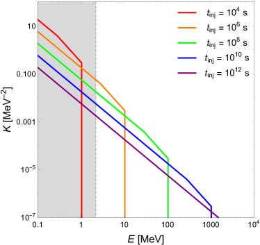
Figure 1: The function $K(E,t_{\mathrm{inj}})$, plotted as a function of photon energy $E$ for several different values of injection time $t_{\mathrm{inj}}$. As discussed in the text, this function determines the shape of the reprocessed photon spectrum for an instantaneous injection of photons of energy $E$ at time $t_{\mathrm{inj}}$. The dashed vertical line at $E\approx 2.2$ MeV indicates the lowest threshold energy associated with any photoproduction or photodisintegration reaction which can significantly alter the abundance of any light nucleus whose primordial abundance is tightly constrained by observation.

One additional complication that we must take into account in assessing the effect of injection on the abundances of light nuclei is that the reprocessed photon spectrum established by Class-I processes immediately after injection at $t_{\mathrm{inj}}$ is subsequently degraded by Class-III processes, which slowly act to bring this reprocessed spectrum into thermal equilibrium with the background photons in the radiation bath. The timescale $\delta t_{\mathrm{th}}(E,t_{\mathrm{inj}})$ on which these processes act on a photon of energy $E$ is roughly

$$\delta t_{\mathrm{th}}(E,t_{\mathrm{inj}})~{}\approx~{}\left[n_{B}(t_{\mathrm{inj}})\sigma_{\mathrm{th}}(E)\right]^{-1}~{},$$ (6)

where $n_{B}(t_{\mathrm{inj}})$ is the number density of baryons at the time of injection and where $\sigma_{\mathrm{th}}(E)$ is the characteristic cross-section for the relevant scattering processes, which include Compton scattering and $e^{+}e^{-}$ pair production off nuclei. The cross-sections for all relevant individual contributing processes can be found in Ref. KawasakiMoroi . Note that while at low energies $\sigma_{\mathrm{th}}(E)$ is well approximated by the Thomson cross-section, this approximation breaks down at higher energies as other processes become relevant.

Given these observations, the spectrum of the resulting non-thermal population of photons at time $t$ not only represents the sum of all contributions from injection at all times $t_{\mathrm{inj}}<t$ but also reflects the subsequent degradation of these contributions by the Class-III processes which serve to thermalize this population of photons with the radiation bath. This overall non-thermal photon spectrum takes the form

$$\frac{dn_{\gamma}(E,t)}{dE} = \int_{0}^{t}\frac{dn_{\gamma}(E,t_{\mathrm{inj}})}{dEdt_{\mathrm{inj}}}G(t,t_{\mathrm{inj}})dt_{\mathrm{inj}}~{},$$ (7)

where

$$G(t,t_{\mathrm{inj}})~{}\equiv~{}e^{-(t-t_{\mathrm{inj}})/\delta t_{\mathrm{th}}(E,t_{\mathrm{inj}})}\Theta(t-t_{\mathrm{inj}})$$ (8)

is the Green’s function which solves the differential equation

$$\frac{dG(t,t_{\mathrm{inj}})}{dt}+\frac{G(t,t_{\mathrm{inj}})}{\delta t_{\mathrm{th}}(E,t_{\mathrm{inj}})}~{}=~{}\delta(t-t_{\mathrm{inj}})~{}.$$ (9)

The population of non-thermal photons described by Eq. (7) serves as the source for the initial photoproduction and photodisintegration reactions ultimately responsible for the modification of light-element abundances after BBN.  We shall therefore henceforth refer to photons in this population as “primary” photons.

In what follows, we will find it useful to employ what we shall call the “uniform-decay approximation.” Specifically, we shall approximate the full exponential decay of each dark-sector species $\chi_{i}$ as if the entire population of such particles throughout the universe were to decay precisely at the same time $\tau_{i}$. As we shall see, this will prove critical in allowing us to formulate our ultimate analytic approximations. We shall nevertheless find that the results of our approximations are generally in excellent agreement with the results of a full numerical analysis.

Within the uniform-decay approximation, the contribution to $d\rho/dt(t_{\mathrm{inj}})$ from the decay of a single unstable particle species $\chi$ takes the form of a Dirac $\delta$-function:

$$\frac{d\rho(t_{\mathrm{inj}})}{dt_{\mathrm{inj}}}~{}=~{}\rho_{\chi}(t_{\mathrm{inj}})\epsilon_{\chi}\delta(t_{\mathrm{inj}}-\tau_{\chi})~{},$$ (10)

where $\rho_{\chi}(t_{\mathrm{inj}})$ is the energy density of $\chi$ at time $t_{\mathrm{inj}}$ and where $\epsilon_{\chi}$ is the fraction of the energy density released by $\chi$ decays which is transferred to photons. It therefore follows that in this approximation, the primary-photon spectrum in Eq. (7) reduces to

$$\frac{dn_{\gamma}(E,t)}{dE} = \rho_{\chi}(\tau_{\chi})\epsilon_{\chi}K(E,\tau_{\chi})$$ (11)

$$\times\,e^{-(t-\tau_{\chi})/\delta t_{\mathrm{th}}(E,t_{\mathrm{inj}})}\Theta(t-\tau_{\chi})~{}.~{}~{}~{}~{}~{}~{}~{}~{}$$

III.2 Light-Element Production/Destruction

Generally speaking, the overall rate of change of the number density $n_{a}$ of a nuclear species $N_{a}$ due to the injection of electromagnetic energy at late times is governed by a Boltzmann equation of the form

$$\frac{dn_{a}}{dt}+3Hn_{a}~{}=~{}\mathcal{C}^{(p)}_{a}+\mathcal{C}^{(s)}_{a}~{},$$ (12)

where $H$ is the Hubble parameter and where $\mathcal{C}_{a}^{(p)}$ and $\mathcal{C}_{a}^{(s)}$ are the collision terms associated with two different classes of scattering processes which contribute to this overall rate of change. We shall describe these individual collision terms in detail below. Since $n_{a}$ is affected by Hubble expansion, it is more convenient to work with the corresponding comoving number density $Y_{a}\equiv n_{a}/n_{B}$, where $n_{B}$ denotes the total number density of baryons. The Boltzmann equation for $Y_{a}$ then takes the form

$$\frac{dY_{a}}{dt}~{}=~{}\frac{1}{n_{B}}\left[\mathcal{C}^{(p)}_{a}+\mathcal{C}^{(s)}_{a}\right]~{}.~{}~{}~{}$$ (13)

The collision term $\mathcal{C}_{a}^{(p)}$ represents the collective contribution from Class-II processes directly involving the population of primary photons described by Eq. (11). The principal processes which contribute to $\mathcal{C}_{a}^{(p)}$ are photoproduction processes of the form $N_{b}+\gamma\rightarrow N_{a}+N_{c}$ and photodisintegration processes of the form $N_{a}+\gamma\rightarrow N_{b}+N_{c}$, where $N_{b}$ and $N_{c}$ are other nuclei in the thermal plasma. The collision term associated with these processes takes the form

$$\mathcal{C}_{a}^{(p)} = \sum_{b,c}\left[Y_{b}n_{B}\!\int_{E_{b}^{(ac)}}^{E_{C}}\!\!\!\frac{dn_{\gamma}(E,t)}{dE}\sigma_{b}^{(ac)}\!(E)dE\right.$$ (14)

$$-\left.Y_{a}n_{B}\!\int_{E_{a}^{(bc)}}^{E_{C}}\!\!\!\frac{dn_{\gamma}(E,t)}{dE}\sigma_{a}^{(bc)}\!(E)dE\right]~{},~{}~{}~{}~{}~{}~{}~{}$$

where the indices $b$ and $c$ run over the nuclei present in the plasma, where $\sigma_{b}^{(ac)}(E)$ and $\sigma_{a}^{(bc)}(E)$ respectively denote the cross-sections for the corresponding photoproduction and photodisintegration processes discussed above, and where $E_{b}^{(ac)}$ and $E_{a}^{(bc)}$ are the respective energy thresholds for these processes. Expressions for these cross-sections and values for the corresponding energy thresholds can be found, e.g., in Ref. CyburtEllisUpdated .

By contrast, $\mathcal{C}_{a}^{(s)}$ represents the collective contribution from additional, secondary processes which involve not the primary photons themselves but rather a non-thermal population of energetic nuclei produced by interactions involving those primary photons. In principle, these secondary processes include both reactions that produce nuclei of species $N_{a}$ and reactions which destroy them. In practice, however, because the non-thermal population of any given species $N_{b}$ generated by processes involving primary photons is comparatively small, the effect of secondary processes on the populations of most nuclear species is likewise small. As we shall discuss in more detail in Sect. III.3, the only exception is $\ce{{}^{6}Li}$, which is not produced in any significant amount during the BBN epoch but which can potentially be produced by secondary processes initiated by photon injection at subsequent times. Since these processes involve the production rather than the destruction of $\ce{{}^{6}Li}$, we focus on the effect of secondary processes on nuclei which appear in the final state rather than the initial state in what follows.

The energetic nuclei which participate in secondary processes are the products of the same kinds of reactions which lead to the collision term in Eq. (14). Thus, the kinetic-energy spectrum $d\widetilde{n}_{b}(E_{b},t)/dE_{b}$ of the non-thermal population of a nuclear species $N_{b}$ produced in this manner is in large part determined by the energy spectrum of the primary photons. In calculating this spectrum, one must in principle account for the fact that a photon of energy $E_{\gamma}$ can give rise to a range of possible $E_{b}$ values due to the range of possible scattering angles between the three-momentum vectors of the incoming photon and the excited nucleus in the center-of-mass frame. However, it can be shown SecProdKinematicsToAppear that a reasonable approximation for the collision term $\mathcal{C}^{(s)}_{a}$ for $\ce{{}^{6}Li}$ is nevertheless obtained by taking $E_{b}$ to be a one-to-one function of $E_{\gamma}$ of the form JedamzikLi6

$$E_{b}~{}=~{}\mathcal{E}(E_{\gamma})~{}\equiv~{}\frac{1}{4}\Big{[}E_{\gamma}-E_{c}^{(bd)}\Big{]}~{},$$ (15)

where $E_{c}^{(bd)}$ is the energy threshold for the primary process $N_{c}+\gamma\rightarrow N_{b}+N_{d}$. In this approximation, $d\widetilde{n}_{b}(E_{b},t)/dE_{b}$ takes the form CyburtEllisUpdated

$$\frac{d\widetilde{n}_{b}(E_{b},t)}{dE_{b}} = \sum_{c,d}\frac{n_{c}}{b(E_{b},t)}\int_{E_{\mathrm{min}}(E_{b})}^{E_{C}}\Bigg{[}\frac{dn_{\gamma}(E_{\gamma}^{\prime},t)}{dE_{\gamma}^{\prime}}~{}~{}~{}$$ (16)

$$~{}\times\sigma^{(bd)}_{c}(E_{\gamma}^{\prime})e^{-\beta_{b}(E_{\gamma}^{\prime},t)}\Bigg{]}dE_{\gamma}^{\prime}~{},~{}~{}~{}~{}~{}$$

where $b(E_{b},t)$ is the energy-loss rate for $N_{b}$ due to Coulomb scattering with particles in the thermal background plasma. The exponential factor $\beta_{b}(E_{\gamma}^{\prime},t)$ accounts for the collective effect of additional processes which act to reduce the number of nuclei of species $N_{b}$. The lower limit of integration in Eq. (16) is given by $E_{\mathrm{min}}(E_{b})=\max[\mathcal{E}^{-1}(E_{b}),E_{c}^{(bd)}]$, where $\mathcal{E}^{-1}(E_{b})$ is the inverse of the function defined in Eq. (15). In other words, $\mathcal{E}^{-1}(E_{b})$ is the photon energy which corresponds to a kinetic energy $E_{b}$ for the excited nucleus.

In principle, the processes which contribute to $\beta_{a}(E_{\gamma}^{\prime},t)$ include both decay processes (in the case in which $N_{b}$ is unstable) and photodisintegration processes of the form $N_{b}+\gamma\rightarrow N_{c}+N_{d}$ involving a primary photon. In practice, the photodisintegration rate due to these processes is much slower that the energy-loss rate due to Coulomb scattering for any species of interest. Moreover, as we shall see in Sect. III.3, the only nuclear species whose non-thermal population has a significant effect on the $\ce{{}^{6}Li}$ abundance are tritium ($\ce{T}$) and the helium isotope $\ce{{}^{3}He}$. Because these two species are mirror nuclei, the secondary processes in which they participate affect the $\ce{{}^{6}Li}$ abundance in the same way and have almost identical cross-sections and energy thresholds. Thus, in terms of their effect on the production of $\ce{{}^{6}Li}$, the populations of $\ce{T}$ and $\ce{{}^{3}He}$ may effectively be treated together as if they were the population of a single nuclear species. Although tritium is unstable and decays via beta decay to $\ce{{}^{3}He}$ with a lifetime of $\tau_{\ce{T}}\approx 5.6\times 10^{8}$ s, these decays have no impact on the combined population of $\ce{T}$ and $\ce{{}^{3}He}$. We may therefore safely approximate $\beta_{b}(E_{\gamma}^{\prime},t)\approx 0$ for this combined population of excited nuclei in what follows.

The most relevant processes through which an energetic nucleus $N_{b}$ in this non-thermal population can alter the abundance of another nuclear species $N_{b}$ are scattering processes of the form $N_{b}+N_{f}\rightarrow N_{a}+X$, in which an energetic nucleus $N_{b}$ from the non-thermal population generated by primary processes scatters with a background nucleus $N_{f}$, resulting in the production of a nucleus of species $N_{a}$ and some other particle $X$ (which could be either an additional nucleus or a photon). In principle, processes of the form $N_{b}+N_{a}\rightarrow N_{f}+X$ can also act to reduce the abundance of $N_{a}$. However, as discussed above, this reduction has a negligible impact on $Y_{a}$ for any nuclear species $N_{a}$ which already has a sizable comoving number density at the end of BBN.  Thus, we focus here on production rather than destruction when assessing the impact of secondary processes on the primordial abundances of light nuclei.

With this simplification, the collision term associated with secondary production processes takes the form

$$\mathcal{C}_{a}^{(s)} = \sum_{b,f}Y_{f}n_{B}\!\int_{E_{bf}^{(aX)}}^{\mathcal{E}(E_{C})}\Bigg{[}\frac{d\widetilde{n}_{b}(E_{b},t)}{dE_{b}}$$ (17)

$$~{}~{}~{}~{}~{}~{}~{}~{}\times\sigma_{bf}^{(aX)}(E_{b})|v(E_{b})|\Bigg{]}dE_{b}~{},~{}~{}~{}$$

where $v(E_{b})$ is the (non-relativistic) relative velocity of nuclei $N_{b}$ and $N_{f}$ in the background frame, where $d\widetilde{n}_{b}(E_{b},t)/dE_{b}$ is the differential energy spectrum of the non-thermal population of $N_{b}$, where $\sigma_{bf}^{(aX)}$ is the cross-section for the scattering process $N_{b}+N_{f}\rightarrow N_{a}+X$ with corresponding threshold energy $E_{bf}^{(aX)}$, and where $\mathcal{E}(E_{C})$ is the cutoff in $d\widetilde{n}_{b}(E_{b},t)/dE_{b}$ produced by primary processes.

III.3 Constraints on Primordial Light-Element Abundances

The nuclear species whose primordial abundances are the most tightly constrained by observation — and which are therefore relevant for constraining the late decays of unstable particles — are $\ce{D}$, $\ce{{}^{4}He}$, $\ce{{}^{6}Li}$, and $\ce{{}^{7}Li}$. The abundance of $\ce{{}^{3}He}$ during the present cosmological epoch has also been constrained by observation BaniaHe3 ; GeissHe3 . However, uncertainties in the contribution to this abundance from stellar sources make it difficult to translate the results of these measurements into bounds on the primordial $\ce{{}^{3}He}$ abundance ChiappiniHe3 ; VangioniFlamHe3 . The effect of these uncertainties can be mitigated in part if we consider the ratio $(\ce{D}+\ce{{}^{3}He})/\ce{H}$ rather than $\ce{{}^{3}He}/\ce{H}$, as the former is expected to be largely unaffected by stellar processing Ellis:1984er ; IoccoBBNReview ; CocBBNReview . In this paper, we focus our attention on $\ce{D}$, $\ce{{}^{4}He}$, $\ce{{}^{6}Li}$, and $\ce{{}^{7}Li}$, as the relationship between the measured abundances of these nuclei and their corresponding primordial abundances is more transparent.

The observational constraints on the primordial abundances of these nuclei can be summarized as follows. Bounds on the primordial $\ce{{}^{4}He}$ abundance are typically phrased in terms of the primordial helium mass fraction $Y_{p}\equiv(\rho_{\ce{{}^{4}He}}/{\rho_{B}})_{p}$, where $\rho_{\ce{{}^{4}He}}$ is the mass density of $\ce{{}^{4}He}$, where $\rho_{B}$ is the total mass density of baryonic matter, and where the subscript $p$ signifies that it is only the primordial contribution to $\rho_{\ce{{}^{4}He}}$ which is used in calculating $Y_{p}$, with subsequent modifications to this quantity due to stellar synthesis, etc., ignored. The $2\sigma$ limits on $Y_{p}$ are AverHe4

$$0.2369~{}<~{}Y_{p}~{}<~{}0.2529~{}.$$ (18)

The observational $2\sigma$ limits on the $\ce{{}^{7}Li}$ abundance are SbordoneLi7

$$1.0\times 10^{-10}~{}<~{}\left(\frac{\ce{{}^{7}Li}}{\ce{H}}\right)_{p}~{}<~{}2.2\times 10^{-10}~{},$$ (19)

where the symbols $\ce{{}^{7}Li}$ and $\ce{H}$ denote the primordial number densities of the corresponding nuclear species. In this connection, we note that significant tension exists between these observational bounds and the predictions of theoretical calculations of the $\ce{{}^{7}Li}$ abundance, which are roughly a factor of three larger. While it is not our aim in this paper to address this discrepancy, electromagnetic injection from the late decays of unstable particles may play a role KusakabeAxion ; EllisParticleDecaysAndLi7 ; KusakabeLi6andLi7 in reconciling these predictions with observational data.

Constraining the primordial abundance of $\ce{D}$ is complicated by a mild tension which currently exists between the observational results for $\ce{D}/\ce{H}$ derived from measurements of the line spectra of low-metallicity gas clouds CookeDUpper and the results obtained from numerical analysis of the Boltzmann equations for BBN MarcucciDLower with input from Planck data Planck2015 , which predict a slightly lower value for this ratio. We account for these tensions by choosing our central value and lower limit on $\ce{D}/\ce{H}$ in accord with the central value and $2\sigma$ lower limit from numerical calculations, while at the same time adopting the $2\sigma$ observational upper limit as our own upper limit on this ratio. Thus, we take our bounds on the $\ce{D}$ abundance to be

$$2.317\times 10^{-5}~{}<~{}\left(\frac{\ce{D}}{\ce{H}}\right)_{p}~{}<~{}2.587\times 10^{-5}~{}.$$ (20)

An upper bound on the ratio $\ce{{}^{6}Li}/\ce{H}$ can likewise be derived from observation by combining observational upper bounds on the more directly constrained quantities $\ce{{}^{6}Li}/\ce{{}^{7}Li}$ and $\ce{{}^{7}Li}/\ce{H}$. By combining the upper bound on $\ce{{}^{6}Li}/\ce{{}^{7}Li}$ from Ref. AsplundLi6toLi7 with the upper bound from Eq. (19), we obtain

$$\left(\frac{\ce{{}^{6}Li}}{\ce{H}}\right)_{p}~{}<~{}2\times 10^{-11}~{}.$$ (21)

While this upper bound is identical to the corresponding constraint quoted in Ref. CyburtEllisUpdated , this is a numerical accident resulting from a higher estimate of the $\ce{{}^{6}Li}/\ce{{}^{7}Li}$ ratio (due to the recent detection of additional $\ce{{}^{6}Li}$ in low-metallicity stars) and a reduction in the upper bound on the $\ce{{}^{7}Li}/{\ce{H}}$ ratio.

Having assessed the observational constraints on $\ce{D}$, $\ce{{}^{4}He}$, $\ce{{}^{6}Li}$, and $\ce{{}^{7}Li}$, we now turn to consider the effect that the late-time injection of electromagnetic radiation has on the abundance of each of these nuclear species relative to its initial abundance at the conclusion of the BBN epoch.

Of all these species, $\ce{{}^{4}He}$ is by far the most abundant. For this reason, reactions involving $\ce{{}^{4}He}$ nuclei in the initial state play an outsize role in the production of other nuclear species. Moreover, since the abundances of all other such species in the thermal bath are far smaller than that of $\ce{{}^{4}He}$, reactions involving these other nuclei in the initial state have a negligible impact on the $\ce{{}^{4}He}$ abundance. Photodisintegration processes initiated directly by primary photons are therefore the only processes which have an appreciable effect on the primordial abundance of $\ce{{}^{4}He}$. A number of individual such processes contribute to the overall photodisintegration rate of $\ce{{}^{4}He}$, all of which have threshold energies $E_{\mathrm{thresh}}\gtrsim 20~{}\,{\rm MeV}$.

The primordial abundance of $\ce{{}^{7}Li}$, like that of $\ce{{}^{4}He}$, evolves in response to photon injection primarily as a result of photodisintegration processes initiated directly by primary photons. At early times, when the energy ceiling $E_{C}$ in Eq. (5) for the spectrum of these photons is relatively low, the process $\ce{{}^{7}Li}+\gamma\rightarrow\ce{{}^{4}He}+\ce{T}$, which has a threshold energy of only $\sim 2.5~{}\,{\rm MeV}$, dominates the photodisintegration rate. By contrast, at later times, additional processes with higher threshold energies, such as $\ce{{}^{7}Li}+\gamma\rightarrow\ce{{}^{6}Li}+n$ and $\ce{{}^{7}Li}+\gamma\rightarrow\ce{{}^{4}He}+2n+p$, become relevant.

While the reactions which have a significant impact on the $\ce{{}^{4}He}$ and $\ce{{}^{7}Li}$ abundances all serve to reduce these abundances, the reactions which have an impact on the $\ce{D}$ abundance include both processes which create deuterium nuclei and processes which destroy them. At early times, photodisintegration processes initiated by primary photons — and in particular the process $\ce{D}+\gamma\rightarrow n+p$, which has a threshold energy of only $E_{\mathrm{thresh}}\approx 2.2~{}\,{\rm MeV}$ — dominate and serve to deplete the initial $\ce{D}$ abundance. At later times, however, additional processes with higher energy thresholds turn on and serve to counteract this initial depletion. The dominant such process is the photoproduction process $\ce{{}^{4}He}+\gamma\rightarrow\ce{D}+n+p$, which has a threshold energy of $E_{\mathrm{thresh}}\approx 25~{}\,{\rm MeV}$.

Unlike $\ce{{}^{4}He}$, $\ce{{}^{7}Li}$, and $\ce{D}$, the nucleus $\ce{{}^{6}Li}$ is not generated to any significant degree by BBN.  However, a population of $\ce{{}^{6}Li}$ nuclei can be generated after BBN as a result of photon injection at subsequent times. The most relevant processes are $\ce{{}^{7}Li}+\gamma\rightarrow\ce{{}^{6}Li}+n$ and the secondary production processes $\ce{{}^{4}He}+\ce{{}^{3}He}\rightarrow\ce{{}^{6}Li}+p$ and $\ce{{}^{4}He}+\ce{T}\rightarrow\ce{{}^{6}Li}+n$, where $\ce{T}$ denotes a tritium nucleus. All of these processes have energy thresholds $E_{\mathrm{thresh}}\approx 7~{}\,{\rm MeV}$. The abundances of $\ce{{}^{3}He}$ and $\ce{T}$, which serve as reactants in these secondary processes, are smaller at the end of BBN than the abundance of $\ce{{}^{4}He}$ by factors of $\mathcal{O}(10^{4})$ and $\mathcal{O}(10^{6})$, respectively (for reviews, see, e.g., Ref. PospelovReview ). At the same time, the non-thermal populations of $\ce{{}^{3}He}$ and $\ce{T}$ generated via the photodisintegration of $\ce{{}^{4}He}$ are much larger than the non-thermal population of $\ce{{}^{4}He}$, which is generated via the photodisintegration of other, far less abundant nuclei. Thus, to a very good approximation, the reactions which contribute to the secondary production of $\ce{{}^{6}Li}$ involve an excited $\ce{{}^{3}He}$ or $\ce{T}$ nucleus and a “background” $\ce{{}^{4}He}$ nucleus in thermal equilibrium with the radiation bath.

In Table 1, we provide a list of the relevant reactions which can serve to alter the abundances of light nuclei as a consequence of photon injection at late times, along with their corresponding energy thresholds. Expressions for the cross-sections for these processes are given in Ref. CyburtEllisUpdated . We note that alternative parametrizations for some of the relevant cross-section formulae have been proposed PramHe4PhotodestructXSec on the basis of recent nuclear experimental results, though tensions still exist among data from different sources. While there exist additional nuclear processes beyond those listed in Table 1 that in principle contribute to the collision terms in Eq. (13), these processes do not have a significant impact on the $Y_{a}$ of any relevant nucleus when the injected energy density is small and can therefore be neglected. In should be noted that the population of excited $\ce{T}$ and $\ce{{}^{3}He}$ nuclei which participate in the secondary production of $\ce{{}^{6}Li}$ are generated primarily by the same processes which contribute to the destruction of $\ce{{}^{4}He}$. We note that we have not included processes which contribute to the destruction of $\ce{{}^{6}Li}$. The reason is that the collision terms for these processes are proportional to $Y_{\ce{{}^{6}Li}}$ itself and thus only become important in the regime in which the rate of electromagnetic injection from unstable-particle decays is large. By contrast, for reasons that shall be discussed in greater detail below, we focus in what follows primarily on the regime in which injection is small and $\ce{{}^{6}Li}$-destruction processes are unimportant. However, we note that these processes can have an important effect on $Y_{\ce{{}^{6}Li}}$ in the opposite regime, rendering the bound in Eq. (21) essentially unconstraining for sufficiently large injection rates CyburtEllisUpdated .

Process	Associated Reactions	$E_{\mathrm{thresh}}$
D Destruction	$\ce{D}+\gamma\rightarrow n+p$	$2.2\,{\rm MeV}$
D Production	$\ce{{}^{4}He}+\gamma\rightarrow\ce{D}+n+p$	$26.1\,{\rm MeV}$
^4He Destruction	$\ce{{}^{4}He}+\gamma\rightarrow\ce{T}+p$	$19.8\,{\rm MeV}$
	$\ce{{}^{4}He}+\gamma\rightarrow\ce{{}^{3}He}+n$	$20.6\,{\rm MeV}$
^7Li Destruction	$\ce{{}^{7}Li}+\gamma\rightarrow\ce{{}^{4}He}+\ce{T}$	$2.5\,{\rm MeV}$
	$\ce{{}^{7}Li}+\gamma\rightarrow\ce{{}^{6}Li}+n$	$7.2\,{\rm MeV}$
	$\ce{{}^{7}Li}+\gamma\rightarrow\ce{{}^{4}He}+2n+p$	$10.9\,{\rm MeV}$
Primary ^6Li Production	$\ce{{}^{7}Li}+\gamma\rightarrow\ce{{}^{6}Li}+n$	$7.2\,{\rm MeV}$
Secondary ^6Li Production	$\ce{{}^{4}He}+\ce{{}^{3}He}\rightarrow\ce{{}^{6}Li}+p$	$7.0\,{\rm MeV}$
	$\ce{{}^{4}He}+\ce{T}\rightarrow\ce{{}^{6}Li}+n$	$8.4\,{\rm MeV}$

Table 1:  Reactions which alter the abundances of $\ce{D}$, $\ce{{}^{4}He}$, $\ce{{}^{6}Li}$, and $\ce{{}^{7}Li}$ in scenarios involving photon injection at late times, along with the corresponding energy threshold $E_{\mathrm{thresh}}$ for each process. We note that the excited $\ce{T}$ and $\ce{{}^{3}He}$ nuclei which participate in the secondary production of $\ce{{}^{6}Li}$ are generated primarily by the processes listed above which contribute to the destruction of $\ce{{}^{4}He}$.

Finally, we note that the rates and energy thresholds for $\ce{{}^{4}He}+\ce{{}^{3}He}\rightarrow\ce{{}^{6}Li}+p$ and $\ce{{}^{4}He}+\ce{T}\rightarrow\ce{{}^{6}Li}+n$ are very similar, as are the rates and energy thresholds for the $\ce{{}^{4}He}$-destruction processes which produce the non-thermal populations of $\ce{{}^{3}He}$ and $\ce{T}$ CyburtEllisUpdated . In what follows, we shall make the simplifying approximation that $\ce{{}^{3}He}$ and $\ce{T}$ are “interchangeable” in the sense that we treat these rates — and hence also the non-thermal spectra $d\widetilde{n}_{a}(E,t)/dE$ of $\ce{{}^{3}He}$ and $\ce{T}$ — as identical. Thus, although $\ce{T}$ decays via beta decay to $\ce{{}^{3}He}$ on a timescale $\tau_{\ce{T}}\approx 10^{8}$ s, we neglect the effect of the decay kinematics on the resulting non-thermal $\ce{{}^{3}He}$ spectrum. As we shall see, these simplifying approximations do not significantly impact our results.

III.4 Towards an Analytic Approximation: Linearization and Decoupling

In order to assess whether a particular injection history is consistent with the constraints discussed in the previous section, we must evaluate the overall change $\delta Y_{a}(t)\equiv Y_{a}(t)-Y_{a}^{\mathrm{init}}$ in the comoving number density $Y_{a}$ of a given nucleus at time $t=t_{\mathrm{now}}$, where $Y_{a}^{\mathrm{init}}$ denotes the initial value of $Y_{a}$ at the end of BBN.  In principle, this involves solving a system of coupled differential equations, one for each nuclear species present in the thermal bath, each of the form given in Eq. (13).

In practice, however, we can obtain reasonably reliable estimates for the $\delta Y_{a}$ without having to resort to a full numerical analysis. This is possible ultimately because observational constraints require $|\delta Y_{a}|$ to be quite small for all relevant nuclei, as we saw in Sect. III.3. The equations governing the evolution of the $Y_{a}$ are coupled due to feedback effects in which a change in the comoving number density of one nuclear species $N_{a}$ alters the reaction rates associated with the production of other nuclear species. However, if the change in $Y_{a}$ is sufficiently small for all relevant species, these feedback effects can be neglected and the evolution equations effectively decouple.

In order for the evolution equations for a particular nuclear species $N_{a}$ to decouple, the linearity criterion $|\delta Y_{b}|\ll Y_{b}$ must be satisfied for any other nuclear species $N_{b}\neq N_{a}$ which serves as a source for reactions that significantly affect the abundance of $N_{a}$ at all times after the conclusion of the BBN epoch. In principle, there are two ways in which this criterion could be enforced by the observational constraints and consistency conditions discussed in Sect. III.3. The first is simply that the applicable bound on each $Y_{b}$ which serves as a source for $N_{a}$ is sufficiently stringent that this bound is always violated before the linearity criterion $|\delta Y_{b}|\ll Y_{b}$ fails. The second possibility is that while the direct bound on $Y_{b}$ may not in and of itself require that $|\delta Y_{b}|$ be small, the comoving number densities $Y_{a}$ and $Y_{b}$ are nevertheless directly related in such a way that the applicable bound on $Y_{a}$ is always violated before the linearity criterion $|\delta Y_{b}|\ll Y_{b}$ fails. If one of these two conditions is satisfied for every species $N_{b}$ which serves as a source for $N_{a}$, we may treat the evolution equation for $N_{a}$ as effectively decoupled from the equations which govern the evolution of all other nuclear species. We emphasize that $N_{a}$ itself need not satisfy the linearity criterion in order for its evolution equation to decouple in this way.

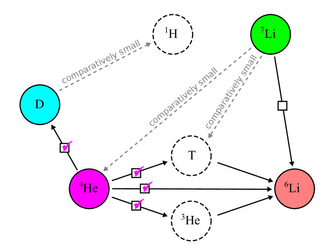
Figure 2: Schematic illustrating the network of reactions precipitated by electromagnetic injection after the end of the BBN epoch. The nodes in the network represent different nuclear species: nodes represented by solid circles correspond to nuclei whose primordial comoving number densities $Y_{a}$ are reliably constrained by data, while nodes represented by dashed circles correspond to other nuclear species involved in these reactions. An arrow pointing from one node to another indicates that the nucleus associated with the node from which the arrow originates serves as a source for the nucleus associated with the node to which the arrow points. A solid arrow indicates that the corresponding reaction can potentially have a non-negligible impact on the abundance of the product nucleus, while a dashed arrow indicates that the effect of the corresponding reaction is always negligible. Note that $\ce{{}^{1}H}$ nuclei — i.e., protons — are generated as a byproduct of many of the other reactions shown. However, the impact of these contributions to the $\ce{{}^{1}H}$ abundance is negligible and the corresponding arrows have been omitted for clarity. A checked box superimposed on the arrows emerging from a node indicates that observational constraints enforce the linearity criterion $|\delta Y_{a}|\ll Y_{a}$ for the corresponding nucleus. By contrast, an open box indicates that this criterion is not satisfied. The Boltzmann equation for a given nucleus $N_{a}$ effectively decouples, in the sense that feedback effects can be neglected in calculating $Y_{a}$, whenever the linearity criterion is satisfied for all $N_{b}\neq N_{a}$ which serve as a source for $N_{a}$ (though not necessarily for $N_{a}$ itself). Since no other nucleus serves as a source for $\ce{{}^{4}He}$ or $\ce{{}^{7}Li}$, the Boltzmann equations for both of these species trivially decouple. The Boltzmann equation for $\ce{D}$ also decouples because $\ce{{}^{4}He}$, the one nucleus which serves as a significant source for $\ce{D}$, is required to satisfy the linearity criterion. However, the Boltzmann equation for $\ce{{}^{6}Li}$ does not decouple, as one of its source nuclei — in particular, $\ce{{}^{7}Li}$ — does not satisfy the linearity criterion. Further details are described in the text.

We now turn to examine whether and under what circumstances our criterion for the decoupling of the evolution equations is satisfied in practice for all relevant nuclear species. In Fig. 2 we illustrate the network of reactions which can have a significant effect on the values of $Y_{a}$ for these species. The nuclei which appear in the initial state of one of the primary production processes listed in Table 1 are $\ce{{}^{4}He}$, which serves as a source for $\ce{D}$ and $\ce{{}^{6}Li}$, and $\ce{{}^{7}Li}$, which serves as a source for $\ce{{}^{6}Li}$. We note that while $\ce{{}^{3}He}$ and $\ce{T}$ each appear in the initial state of one of the secondary production processes for $\ce{{}^{6}Li}$, it is the non-thermal population of each nucleus which plays a significant role in these reactions. Since the non-thermal populations of both $\ce{{}^{3}He}$ and $\ce{T}$ are generated primarily as a byproduct of $\ce{{}^{4}He}$ destruction, requiring that the linearity criterion be satisfied for $\ce{{}^{4}He}$ and $\ce{{}^{7}Li}$ is sufficient to ensure that the evolution equations for all relevant nuclear species decouple.

We begin by assessing whether the direct constraints on $Y_{\ce{{}^{4}He}}$ and $Y_{\ce{{}^{7}Li}}$ themselves are sufficient to enforce the linearity criterion. We take the initial values of these comoving number densities at the end of the BBN epoch to be those which correspond to the central observational values for $Y_{p}$ and $\ce{{}^{7}Li}/\ce{H}$ quoted in Ref. CyburtBBN2015 , namely $Y_{p}=0.2449$ and $\ce{{}^{7}Li}/\ce{H}=1.6\times 10^{-10}$. Since neither $\ce{{}^{4}He}$ nor $\ce{{}^{7}Li}$ is produced at a significant rate by interactions involving other nuclear species, the evolution equation in Eq. (13) for each of these nuclei takes the form

$$\frac{dY_{b}}{dt}~{}=~{}-Y_{b}(t)\Gamma_{b}(t)~{},$$ (22)

where the quantity $\Gamma_{b}(t)\equiv-\mathcal{C}_{b}^{(p)}/Y_{b}n_{B}\geq 0$ represents the rate at which $Y_{b}$ is depleted as a result of photodisintegration processes. This depletion rate varies in time, but depends neither on $Y_{b}$ nor on the comoving number density of any other nucleus. Since $Y_{b}$ decreases monotonically in this case, it follows that if this comoving quantity lies within the observationally-allowed range today, it must also lie within this range at all times since the end of the BBN epoch.

The bound on $Y_{\ce{{}^{4}He}}$ which follows from Eq. (18) is sufficiently stringent that $|\delta Y_{\ce{{}^{4}He}}|\ll Y_{\ce{{}^{4}He}}$ is indeed required at all times since the end of BBN for consistency with observation. Thus, our linearity criterion is always satisfied for $\ce{{}^{4}He}$. By contrast, the bound on $Y_{\ce{{}^{7}Li}}$ in Eq. (19) is far weaker in the sense that $|\delta Y_{\ce{{}^{7}Li}}|$ need not necessarily be small in relation to $Y_{\ce{{}^{7}Li}}$ itself. Moreover, while the contribution to $\delta Y_{\ce{{}^{6}Li}}$ from primary production is indeed directly related to $\delta Y_{\ce{{}^{7}Li}}$, we find that the observational bound on $Y_{\ce{{}^{6}Li}}$ is not always violated before the linearity criterion $|\delta Y_{\ce{{}^{7}Li}}|\ll Y_{\ce{{}^{7}Li}}$ fails — even if we assume $Y_{\ce{{}^{6}Li}}\approx 0$ at the end of BBN.  The reason is that not every $\ce{{}^{7}Li}$ nucleus destroyed by primary photodisintegration processes produces a $\ce{{}^{6}Li}$ nucleus. Indeed, $\ce{{}^{7}Li}+\gamma\rightarrow\ce{{}^{4}He}+\ce{T}$ and $\ce{{}^{7}Li}+\gamma\rightarrow\ce{{}^{4}He}+2n+p$ contribute to the depletion of $Y_{\ce{{}^{7}Li}}$ as well.

Since the energy threshold for $\ce{{}^{7}Li}+\gamma\rightarrow\ce{{}^{4}He}+\ce{T}$ is lower than the threshold for $\ce{{}^{7}Li}+\gamma\rightarrow\ce{{}^{6}Li}+n$, there will be a range of $t_{\mathrm{inj}}$ within which injection contributes to the destruction of $\ce{{}^{7}Li}$ without producing $\ce{{}^{6}Li}$ at all. Furthermore, even at later injection times $t_{\mathrm{inj}}\gtrsim 4.9\times 10^{5}$ s, when the primary-photon spectrum from injection includes photons with energies above the threshold for $\ce{{}^{7}Li}+\gamma\rightarrow\ce{{}^{6}Li}+n$, the $\ce{{}^{7}Li}$-photodisintegration rates associated with this process and the rates associated with $\ce{{}^{7}Li}+\gamma\rightarrow\ce{{}^{4}He}+\ce{T}$ and $\ce{{}^{7}Li}+\gamma\rightarrow\ce{{}^{4}He}+2n+p$ are comparable. Consequently, only around 30% of $\ce{{}^{7}Li}$ nuclei destroyed by primary photodisintegration for $t_{\mathrm{inj}}\gtrsim 4.9\times 10^{5}$ s produce a $\ce{{}^{6}Li}$ nucleus in the process. Thus, a large $|\delta Y_{\ce{{}^{7}Li}}|$ invariably results in a much smaller contribution to $\delta Y_{\ce{{}^{6}Li}}$. Thus, $\ce{{}^{7}Li}$ does not satisfy the linearity criterion when serving as a source for $\ce{{}^{6}Li}$.

That said, while our linearity criterion is not truly satisfied for $\ce{{}^{7}Li}$, we can nevertheless derive meaningful constraints on decaying particle ensembles from observational bounds on $\ce{{}^{6}Li}$ by neglecting feedback effects on $Y_{\ce{{}^{7}Li}}$ in calculating $Y_{\ce{{}^{6}Li}}$. Since the Boltzmann equation for $Y_{\ce{{}^{7}Li}}$ takes the form given in Eq. (22), $Y_{\ce{{}^{7}Li}}$ is always less than or equal to its initial value $Y_{\ce{{}^{7}Li}}^{\mathrm{init}}$ at the end of BBN.  This in turn implies that the collision term $\mathcal{C}_{\ce{{}^{6}Li}}^{(p)}$ in the Boltzmann equation for $\ce{{}^{6}Li}$ is always less than or equal to the value that it would have had if the linearity criterion for $\ce{{}^{7}Li}$ had been satisfied. It therefore follows that the contribution to $\delta Y_{\ce{{}^{6}Li}}$ from primary production which we would obtain if we were to approximate $Y_{\ce{{}^{7}Li}}$ by $Y_{\ce{{}^{7}Li}}^{\mathrm{init}}$ at all times subsequent to the end of BBN is always an overestimate. In this sense, then, the bound on electromagnetic injection which we would obtain by invoking this linear approximation for $Y_{\ce{{}^{7}Li}}$ represents a conservative bound. Moreover, it turns out that because of the relationship between $Y_{\ce{{}^{7}Li}}$ and $Y_{\ce{{}^{6}Li}}$, the bound on decaying ensembles from the destruction of $\ce{{}^{7}Li}$ is always more stringent than the bound from the primary production of $\ce{{}^{6}Li}$. Thus, adopting the linear approximation for $\ce{{}^{7}Li}$ in calculating $\mathcal{C}_{\ce{{}^{6}Li}}^{(p)}$ does not artificially exclude any region of parameter space for such ensembles once the combined constraints from all relevant nuclear species are taken into account.

Motivated by these considerations, in what follows we shall therefore adopt the linear approximation in which $Y_{b}\approx Y_{b}^{\mathrm{init}}$ in calculating the collision terms $\mathcal{C}_{a}^{(p)}$ and $\mathcal{C}_{a}^{(s)}$ for any nuclear species $N_{a}\neq N_{b}$ for which $N_{b}$ serves as a source. As we have seen, this approximation is valid for all species except for $\ce{{}^{7}Li}$, which serves as a source for primary $\ce{{}^{6}Li}$ production. Moreover, adopting this approximation for $\ce{{}^{7}Li}$ in calculating $\mathcal{C}_{\ce{{}^{6}Li}}^{(p)}$ yields a conservative bound on electromagnetic injection from decaying particle ensembles.

As discussed above, the advantage of working within the linear approximation is that the Boltzmann equations for all relevant $N_{a}$ effectively decouple and may be solved individually in order to yield analytic approximations for $\delta Y_{a}$. In the simplest case, in which the collision terms $C_{a}^{(p)}$ and $C_{a}^{(s)}$ in the Boltzmann equation for $N_{a}$ include only source terms and not sinks, the right side of Eq. (13) is independent of $Y_{a}$ itself. Thus, within the linear approximation, this equation may be integrated directly, yielding

$$\delta Y_{a}(t)~{}\approx~{}\int_{t_{0}}^{t}\frac{dY_{a}}{dt^{\prime}}dt^{\prime}~{},$$ (23)

where $t_{0}$ represents the time at the conclusion of the BBN epoch beyond which the initial abundance $Y_{a}(t_{0})=Y_{a}^{\mathrm{init}}$ generated by standard primordial nucleosynthesis remains essentially fixed in the absence of any subsequent injection. Moreover, even in cases in which $C_{a}^{(p)}$ and $C_{a}^{(s)}$ include both source and sink terms, we may still evaluate $\delta Y_{a}$ in this way, provided that observational constraints restrict $\delta Y_{a}$ to the region $|\delta Y_{a}|\ll Y_{a}$ and therefore allow us to ignore feedback effects and approximate $Y_{a}\approx Y_{a}^{\mathrm{init}}$ as a constant on the right side of Eq. (13).

Since the Boltzmann equation for $\ce{{}^{6}Li}$ contains no non-negligible sink terms, and since observational constraints require that $|\delta Y_{a}|\ll Y_{a}$ for both $\ce{{}^{4}He}$ and $\ce{D}$, it follows that $\delta Y_{a}$ is well approximated by Eq. (23) for these species. Indeed, the only relevant nucleus which does not satisfy these criteria for direct integration is $\ce{{}^{7}Li}$. Nevertheless, since $\ce{{}^{7}Li}$ is destroyed by a number of primary photodisintegration processes but not produced in any significant amount, the Boltzmann equation for this nucleus takes the particularly simple form specified in Eq. (22). This first-order differential equation can easily be solved for $Y_{a}$, yielding an expression for the comoving number density at any time $t\geq t_{0}$:

$$Y_{a}(t)~{}=~{}Y_{a}^{\mathrm{init}}\exp\left[-\int_{t_{0}}^{t}\!\!\Gamma_{a}(t^{\prime})dt^{\prime}\right]~{}.$$ (24)

When this relation is expressed in terms of $\delta Y_{a}$ rather than $Y_{a}$, we find that it may be recast in the more revealing form

$$Y_{a}^{\mathrm{init}}\ln\left[1+\frac{\delta Y_{a}(t)}{Y_{a}^{\mathrm{init}}}\right] = -Y_{a}^{\mathrm{init}}\!\int_{t_{0}}^{t}\!\!\Gamma_{a}(t^{\prime})dt^{\prime}~{}.~{}~{}~{}$$ (25)

In situations in which the linearity criterion $|\delta Y_{a}(t)|\ll Y_{a}^{\mathrm{init}}$ is satisfied for the nucleus $N_{a}$ itself at all times $t\geq t_{0}$, Taylor expansion of the left side of this equation yields

$$\delta Y_{a}(t) \approx -Y_{a}^{\mathrm{init}}\int_{t_{0}}^{t}\!\!\Gamma_{a}(t^{\prime})dt^{\prime}~{},$$ (26)

which is also the result obtained by direct integration of the Boltzmann equation for $N_{a}$ in the approximation that $Y_{a}\approx Y_{a}^{\mathrm{init}}$.

Comparing Eqs. (25) and (26), we see that if we were to neglect feedback and take $Y_{a}\approx Y_{a}^{\mathrm{init}}$ when evaluating $\delta Y_{a}$ for a species for which this approximation is not particularly good, the naïve result that we would obtain for $\delta Y_{a}$ would in fact correspond to the value of the quantity $Y_{a}^{\mathrm{init}}\ln[1+\delta Y_{a}(t)/Y_{a}^{\mathrm{init}}]$. Thus, given that a dictionary exists between the value of $\delta Y_{a}$ obtained from Eq. (25) and the value obtained from Eq. (26), for simplicity in what follows we shall derive our analytic approximation for $\delta Y_{a}$ using Eq. (26) and simply note that the appropriate substitution should be made for the case of $\ce{{}^{7}Li}$. That said, we also find that the constraint on $\Omega_{\chi}$ that we would derive from Eq. (26) in single-particle injection scenarios from the observational bound on $Y_{\ce{{}^{7}Li}}$ differs from the constraint that we would derive from the more accurate approximation in Eq. (25) by only $\mathcal{O}(10\%)$. Thus, results obtained by approximating $\delta Y_{\ce{{}^{7}Li}}$ by the expression in Eq. (26) are nevertheless fairly reliable in such scenarios — and indeed can be expected to be reasonably reliable in scenarios involving decaying ensembles as well.

III.5 Analytic Approximation: Contribution from Primary Processes

Having discussed how the Boltzmann equations for the relevant $N_{a}$ effectively decouple in the linear regime, we now proceed to derive a set of approximate analytic expressions for $\delta Y_{a}$ from these decoupled equations. We begin by considering the contribution to $\delta Y_{a}$ that arises from primary photoproduction or photodisintegration processes. The contribution from secondary processes, which is relevant only for $\ce{{}^{6}Li}$, will be discussed in Sect. III.6.

Our ultimate goal is to derive an approximate analytic expression for the total contribution to $\delta Y_{a}$ due the injection of photons from an entire ensemble of decaying states. However, our first step in this derivation shall be to consider the simpler case in which the injection is due to the decay of a single unstable particle species $\chi$ with a lifetime $\tau_{\chi}$. We shall work within the uniform-decay approximation, in which the non-thermal photon spectrum takes the particularly simple form in Eq. (11). In this approximation, the lower limit of integration in Eq. (23) may be replaced by $\tau_{\chi}$, while the upper limit can be taken to be any time well after photons at energies above the thresholds $E_{b}^{(ac)}$ and $E_{a}^{(bc)}$ for all relevant photoproduction and photodisintegration processes have thermalized. Thus, we may approximate the change in the comoving number density of each relevant nuclear species as

$$\delta Y_{a}~{}\approx~{}\int_{\tau_{\chi}}^{\infty}\frac{dY_{a}}{dt}dt~{}.$$ (27)

In evaluating each $\delta Y_{a}$, we may also take advantage of the fact that the rates for the relevant reactions discussed in Sect. III.3 turn out to be such that the first (source) and second (sink) terms in Eq. (14) are never simultaneously large for any relevant nuclear species. Indeed, the closest thing to an exception occurs during a very small time interval within which the source and sink terms for $\ce{D}$ are both non-negligible. Thus, depending on the value of $\tau_{\chi}$ and its relationship to the timescales associated with these reactions, we may to a very good approximation treat the effect of injection from a single decaying particle as either producing or destroying $N_{a}$.

With these approximations, the integral over $t$ in Eq. (27) may be evaluated in closed form. In particular, when the source term in Eq. (14) dominates, we find that $\delta Y_{a}$ is given by

$$\delta Y_{a} \approx \sum_{b,c}\frac{Y_{b}\epsilon_{\chi}\rho_{\chi}(\tau_{\chi})}{n_{B}(\tau_{\chi})}$$ (28)

$$~{}~{}\times\int_{E_{b}^{(ac)}}^{E_{C}}dEK(E,\tau_{\chi})S_{b}^{(ac)}(E)~{},~{}~{}~{}$$

where we have defined

$$S_{b}^{(ac)}(E)~{}\equiv~{}\frac{\sigma_{b}^{(ac)}(E)}{\sigma_{\mathrm{th}}(E)}~{}.$$ (29)

By contrast, when the sink term dominates, we find that $\delta Y_{a}$ is given by

$$\delta Y_{a} \approx -\sum_{b,c}\frac{Y_{a}\epsilon_{\chi}\rho_{\chi}(\tau_{\chi})}{n_{B}(\tau_{\chi})}$$ (30)

$$~{}~{}\times\int_{E_{a}^{(bc)}}^{E_{C}}dEK(E,\tau_{\chi})S_{a}^{(bc)}(E)~{}.$$

While the expressions for $\delta Y_{a}$ in Eqs. (30) and (28) pertain to the case of a single unstable particle within the uniform-decay approximation, it is straightforward to generalize these results to more complicated scenarios. Indeed, within the linear approximation, the total change $\delta Y_{a}$ in $Y_{a}$ which results from multiple instantaneous injections over an extended time interval is well approximated by the sum of the individual contributions from these injections. In the limit in which this set of discrete injections becomes a continuous spectrum, this sum becomes an integral over the injection time $t_{\mathrm{inj}}$. Thus, in the continuum limit, $\delta Y_{a}$ is well approximated by

$$\delta Y_{a}~{}\approx~{}\int_{0}^{\infty}\frac{dY_{a}}{dt_{\mathrm{inj}}}dt_{\mathrm{inj}}~{},$$ (31)

where $dY_{a}/dt_{\mathrm{inj}}$ is the differential change in $Y_{a}$ due to an infinitesimal injection of energy in the form of photons at time $t_{\mathrm{inj}}$.

The approximation in Eq. (31) allows us to account for the full exponential time-dependence of the electromagnetic injection due to particle decay in calculating $\delta Y_{a}$ for any given nucleus. By extension, Eq. (31) gives us the ability to compare the results for $\delta Y_{a}$ obtained both with and without invoking the uniform-decay approximation, thereby providing us insight into how reliably $\delta Y_{a}$ can be computed with this approximation.

As an example, let us consider the effect of a single decaying particle $\chi$ with lifetime $\tau_{\chi}$ on the comoving number density of $\ce{{{}^{4}}He}$. Within the uniform-decay approximation, $\delta Y_{\ce{{}^{4}He}}$ is given by Eq. (30) because the sink term in Eq. (14) dominates. By contrast, when the full exponential nature of $\chi$ decay is taken into account, the corresponding result is

$$\delta Y_{a} \approx -\sum_{b,c}\int_{0}^{\infty}dt_{\mathrm{inj}}\Bigg{[}\frac{Y_{a}\epsilon_{\chi}}{n_{B}(t_{\mathrm{inj}})}\frac{d\rho_{\chi}(t_{\mathrm{inj}})}{dt_{\mathrm{inj}}}$$ (32)

$$~{}~{}~{}~{}~{}\times\int_{E_{a}^{(bc)}}^{E_{C}}dEK(E,t_{\mathrm{inj}})S_{c}^{(bd)}(E)\Bigg{]}~{},~{}~{}~{}~{}~{}~{}$$

where $d\rho_{\chi}(t_{\mathrm{inj}})/dt_{\mathrm{inj}}$ denotes the rate of change in the energy density of $\chi$ per unit time $t_{\mathrm{inj}}$. Prior to $t_{\mathrm{MRE}}$, the energy density of an unstable particle with an extrapolated abundance $\Omega_{\chi}$ may be written

$$\rho_{\chi}(t)~{}=~{}\rho_{\mathrm{crit}}(t_{\mathrm{now}})\left(\frac{t_{\mathrm{now}}}{t_{\mathrm{MRE}}}\right)^{2}\left(\frac{t_{\mathrm{MRE}}}{t}\right)^{3/2}\Omega_{\chi}e^{-t/\tau_{\chi}}~{},$$ (33)

where $\rho_{\mathrm{crit}}(t_{\mathrm{now}})$ is the critical density of the universe at present time and where $t_{\mathrm{MRE}}$ is the time of matter-radiation equality. The corresponding rate of change in the energy density, properly evaluated in the comoving frame and then transformed to the physical frame, is

$$\frac{d\rho_{\chi}(t_{\mathrm{inj}})}{dt_{\mathrm{inj}}} = -\rho_{\mathrm{crit}}(t_{\mathrm{now}})\left(\frac{t_{\mathrm{now}}}{t_{\mathrm{MRE}}}\right)^{2}\left(\frac{t_{\mathrm{MRE}}}{t_{\mathrm{inj}}}\right)^{3/2}$$ (34)

$$\times\,\frac{\Omega_{\chi}}{\tau_{\chi}}e^{-t_{\mathrm{inj}}/\tau_{\chi}}~{}.$$

The corresponding expressions for continuum injection in cases in which the source term in Eq. (14) dominates are completely analogous and can be derived in a straightforward way.

In Fig. 3, we compare the results obtained for $\delta Y_{\ce{{}^{4}He}}$ within the uniform-decay approximation to the results obtained with the full exponential time-dependence of $\chi$ decay taken into account. In particular, within the $(\Omega_{\chi},\tau_{\chi})$ plane, we display contours of the corresponding $\ce{{}^{4}He}$ mass fraction $Y_{p}$ obtained within the uniform-decay approximation (upper panel) and through the full exponential calculation (lower panel). For concreteness, in calculating these contours we have assumed an initial value $Y_{p}=0.2449$ for the $\ce{{}^{4}He}$ mass fraction at the end of BBN, following Ref. CyburtBBN2015 .

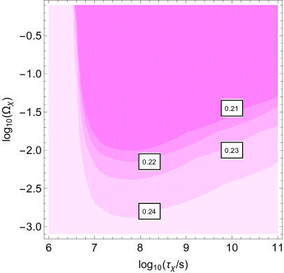
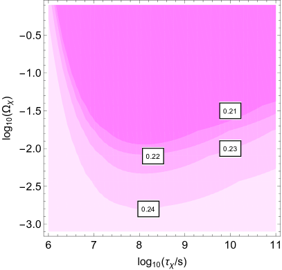
Figure 3: Contours of the primordial $\ce{{}^{4}He}$ mass fraction $Y_{p}$ obtained in the presence of a single decaying particle species $\chi$ with lifetime $\tau_{\chi}$ and extrapolated abundance $\Omega_{\chi}$, plotted within the $(\Omega_{\chi},\tau_{\chi})$ plane. Note that $\Omega_{\chi}$ represents the abundance that $\chi$ would have had at present time if it had not decayed. The upper panel shows the results obtained within the uniform-decay approximation, while the lower panel shows the corresponding results obtained with the full exponential time-dependence of $\chi$ decay taken into account. Comparing the results shown in the two panels, we see that the uniform-decay approximation indeed provides a reasonable approximation for $Y_{p}$.

Comparing the two panels of Fig. 3, we see that the results for $Y_{p}$ obtained within the uniform-decay approximation are indeed very similar throughout most of the parameter space shown to the results obtained through the full calculation. Nevertheless, we observe that discrepancies do arise. For example, we note that the constraints obtained within the uniform-decay approximation are slightly stronger for particles with lifetimes within the range $10^{7}\mbox{~{}s}\lesssim\tau_{\chi}\lesssim 10^{8}\mbox{~{}s}$ and slightly weaker for $\tau_{\chi}$ above this range than the constraints obtained through the full calculation. These discrepancies are ultimately due to the fact that the reprocessed photon spectrum in Eq. (1) depends on the temperature of the radiation bath. Thus, there is a timescale $t_{\sigma,\mathrm{\max}}$ for which the reaction rate for a particular photoproduction or photodisintegration process is maximized for fixed $d\rho(t_{\mathrm{inj}})/dt_{\mathrm{inj}}$. Since all of the energy density $\rho_{\chi}$ initially associated with the decaying particle is injected precisely at $\tau_{\chi}$ within the uniform-decay approximation, this approximation yields slightly more stringent constraints than those obtained through the full calculation when $\tau_{\chi}\sim t_{\sigma,\mathrm{\max}}$. By the same token, the constraints obtained within the uniform-decay approximation are slightly less stringent than those obtained through the full calculation when $\tau_{\chi}$ differs significantly from $t_{\sigma,\mathrm{\max}}$.

We also observe that for lifetimes $\tau_{\chi}\lesssim 10^{7}$ s, the uniform-decay approximation likewise yields constraints that are weaker than those obtained through the full exponential calculation. The reason for this is that the upper energy cutoff $E_{C}$ in the reprocessed photon spectrum is proportional to $t_{\mathrm{inj}}^{1/2}$. For sufficiently early injection times, $E_{C}$ lies below the threshold energy $E_{a}^{(bc)}$ for the photodisintegration reactions which contribute to $\delta Y_{\ce{{}^{4}He}}$. Injection at such early times therefore has essentially no impact on $Y_{p}$. This implies that within the uniform-decay approximation, a particle with a lifetime in this regime likewise has no effect on $Y_{p}$. By contrast, within the full exponential calculation, injection occurs at a significant rate well after $\tau_{\chi}$, leading to a non-negligible change in $Y_{p}$ even when the lifetime of the decaying particle is short.

In summary, the results shown in Fig. 3 indicate that other than in the regime where $\tau_{\chi}$ is sufficiently short that $E_{C}$ lies below the threshold energy for $\ce{{}^{4}He}$ destruction, the result for $\delta Y_{\ce{{}^{4}He}}$ obtained within the uniform-decay approximation is very similar to the result obtained through the full exponential calculation for the same $\tau_{\chi}$ and $\Omega_{\chi}$. We find this to be the case for the other relevant nuclei as well. Thus, having shown that the results for $\delta Y_{a}$ obtained within the uniform-decay approximation accord well with those obtained through the full exponential calculation, at least for sufficiently long $\tau_{\chi}$, we shall adopt this approximation in deriving our constraints on ensembles of electromagnetically-decaying particles. As we shall see, the advantage of working within the uniform-decay approximation is that within this approximation it is possible to write down a simple analytic expression for $\delta Y_{a}$. However, as we shall discuss in more detail below, we shall adopt an alternative strategy for approximating $\delta Y_{a}$ within the regime in which $\tau_{\chi}$ is short and the results obtained within the uniform-decay approximation do not agree with those obtained through the full exponential calculation.

In order to write down our analytic expressions for $\delta Y_{a}$, we shall make one additional approximation: we shall treat the ratio of cross-sections $S_{c}^{(bd)}(E)$ as not varying significantly as a function of energy between the threshold energy $E_{a}^{(bc)}$ and $E_{C}$. When this approximation holds, we may treat this ratio as a constant and pull it outside the integral over photon energies. In order to justify this approximation, we begin by noting that the cross-sections $\sigma_{a}^{(bc)}(E)$ for primary processes typically peak at a value slightly above $E_{a}^{(bc)}$ but fall precipitously with $E$ beyond that point (see, e.g., Ref. CyburtEllisUpdated ). In the vicinity of the peak, however, the variation of $\sigma_{a}^{(bc)}(E)$ is relatively gentle. Since the thermalization cross-section $\sigma_{\mathrm{th}}(E)$ for primary photons varies much less rapidly across the relevant region of $E$, the functional dependence of $S_{a}^{(bc)}(E)$ on $E$ is principally determined by the behavior of $\sigma_{a}^{(bc)}(E)$. Moreover, because $K(E,\tau_{\chi})$ falls rapidly with $E$, the dominant contribution to the energy integral in Eq. (30) arises from photons just above threshold even within the approximation that $S_{a}^{(bc)}(E)$ is constant. Thus, to a good approximation, we may replace $S_{c}^{(bd)}(E)$ by a constant on the order of its peak value and take this quantity outside the energy integral.

Within this approximation, it is now possible to analytically evaluate the integral in Eq. (28). The form of the result depends on the relationship between the threshold energy $E_{a}^{(bc)}$ for the scattering process and the energy scales $E_{C}(t_{\mathrm{inj}})$ and $E_{X}(t_{\mathrm{inj}})$ which determine the shape of the photon spectrum at time $t_{\mathrm{inj}}=\tau_{\chi}$. There are three cases of interest: the case in which $E_{a}^{(bc)}>E_{C}(\tau_{\chi})$, the case in which $E_{C}(\tau_{\chi})>E_{a}^{(bc)}>E_{X}(\tau_{\chi})$, and the case in which $E_{X}(\tau_{\chi})>E_{a}^{(bc)}$. Moreover, the relations in Eq. (5) imply that each of these cases corresponds to a specific range of $\tau_{\chi}$. In particular, the respective lifetime regimes are $\tau_{\chi}<t_{Ca}^{(bc)}$, $t_{Ca}^{(bc)}<\tau_{\chi}<t_{Xa}^{(bc)}$, and $t_{Xa}^{(bc)}<\tau_{\chi}$, where we have defined

$$t_{Ca}^{(bc)} \approx (10^{8}\,{\rm s})\times\left[\frac{E_{a}^{(bc)}}{103\,\,{\rm MeV}}\right]^{2}$$

$$t_{Xa}^{(bc)} \approx (10^{8}\,{\rm s})\times\left[\frac{E_{a}^{(bc)}}{28\,\,{\rm MeV}}\right]^{2}~{}.$$ (35)

Within the $\tau_{\chi}<t_{Ca}^{(bc)}$ regime, none of the photons produced by $\chi$ decay exceed the threshold for the photodisintegration process. The contribution to $\delta Y_{a}$ within the uniform-decay approximation is therefore formally zero. As discussed above, this is the regime in which the uniform-decay approximation fails to reproduce the results obtained through the full exponential calculation. Thus, in order to derive a meaningful bound on decaying particles with lifetimes in this regime, we instead model the injection of photons using the full continuum expression in Eq. (32) with $d\rho(t_{\mathrm{inj}})/dt_{\mathrm{inj}}$ given by Eq. (34). However, in order to arrive at a simple analytic expression for $\delta Y_{a}$, we include only the contribution from injection times in the range $t_{Ca}^{(bc)}<t_{\mathrm{inj}}<t_{Ca}^{(bc)}+\tau_{\chi}$ and drop terms in $\tau_{\chi}/t_{Ca}^{(bc)}$ beyond leading order in the resulting expression. With these approximations, in this regime we find

$$\delta Y_{a}~{}=~{}\sum_{b,c}A_{a}^{(bc)}\Omega_{\chi}\left(\frac{\tau_{\chi}}{t_{Ca}^{(bc)}}\right)e^{-t_{Ca}^{(bc)}/\tau_{\chi}}~{},$$ (36)

where the proportionality constant $A_{a}^{(bc)}$ for each contributing reaction is independent of the properties of the decaying particle. This treatment ensures that we obtain a more reliable estimate for the contribution to $\delta Y_{a}$ from particles with $\tau_{\chi}$ in this regime.

Within the remaining two lifetime regimes, the contribution to $\delta Y_{a}$ within the uniform-decay approximation is non-vanishing. Thus, within these regimes, we obtain our approximation for $\delta Y_{a}$ by integrating Eq. (28), as discussed above. For $t_{Ca}^{(bc)}<\tau_{\chi}<t_{Xa}^{(bc)}$ we find

$$\delta Y_{a}~{}=~{}\sum_{bc}B_{a}^{(bc)}\Omega_{\chi}\left[1-\beta\left(\frac{\tau_{\chi}}{t_{Xa}^{(bc)}}\right)^{\!-1/2}\right]~{},$$ (37)

where $B_{a}^{(bc)}$ is a proportionality constant and where $\beta\equiv E_{X}/E_{C}\approx 0.27$ is the $\tau_{\chi}$-independent ratio of the energy scales in Eq. (5). Likewise, for $t_{Xa}^{(bc)}<\tau_{\chi}$ we find

$$\delta Y_{a} = \sum_{bc}B_{a}^{(bc)}\Omega_{\chi}\left(\frac{\tau_{\chi}}{t_{Xa}^{(bc)}}\right)^{\!-1/4}$$ (38)

$$\times\left[2-(1+\beta)\left(\frac{\tau_{\chi}}{t_{Xa}^{(bc)}}\right)^{\!-1/4}\right]~{}.$$

We emphasize that the proportionality constant $B_{a}^{(bc)}$ for a given process in Eq. (38) is the same as the corresponding proportionality constant in Eq. (37). However, in general $B_{a}^{(bc)}$ differs from the corresponding proportionality constant $A_{a}^{(bc)}$ appearing in Eq. (36).

Strictly speaking, Eq. (38) does not hold for arbitrarily large $\tau_{\chi}$, since photons produced by extremely late decays are not efficiently reprocessed by Class-I processes into the spectrum in Eq. (1). In order to account for this in what follows, we shall consider each term in the sum in Eq. (38) to be valid only for injection times $t_{\mathrm{inj}}<t_{fa}^{(bc)}$, where $t_{fa}^{(bc)}$ is a characteristic cutoff timescale associated with the reaction. Photons injected after this cutoff timescale are assumed to have no effect on $Y_{a}$. For most reactions, it is appropriate to take $t_{fa}^{(bc)}\approx 10^{12}$ s, as this is the timescale beyond which certain crucial Class-I processes effectively begin to shut off and the reprocessed photon spectrum is no longer reliably described by Eq. (1).

III.6 Analytic Approximation: Contribution from Secondary Processes

The approximate analytic expressions for $\delta Y_{a}$ which we have derived in Sect. III.5 are applicable to all of the primary photoproduction or photodisintegration processes relevant for constraining electromagnetic injection from unstable-particle decays after BBN.  However, since secondary production can contribute non-negligibly to the production of $\ce{{}^{6}Li}$, we must derive analogous expressions for $\delta Y_{a}$ in the case of secondary production as well. Moreover, since secondary production is fundamentally different from primary production in terms of particle kinematics, there is no reason to expect that these expressions should have the same functional dependence on $\tau_{\chi}$ as that exhibited by the expressions in Eqs. (36)–(38). Indeed, as we shall see, they do not.

We begin this undertaking by observing that within the uniform-decay approximation, the contribution to $\delta Y_{a}$ from secondary production is given by

$$\delta Y_{a}~{}\approx~{}\!\!\sum_{b,c,d,f}\int_{\tau_{\chi}}^{\infty}\!\!\!\!\!dt\Bigg{\{}Y_{f}\epsilon_{\chi}\rho_{\chi}(\tau_{\chi})\!\int_{E_{bf}^{(aX)}}^{\mathcal{E}(E_{C})}\!\!\!dE_{b}\Bigg{[}\frac{n_{c}(t)\sigma_{bf}^{(aX)}(E)|v(E_{b})|}{b(E_{b},t)}\!\int_{E_{\mathrm{min}}(E_{b})}^{E_{C}}\!\!\!\!\!\!\!\!\!\!dE_{\gamma}K(E_{\gamma},\tau_{\chi})\sigma_{c}^{(bd)}(E_{\gamma})e^{-\frac{(t-\tau_{\chi})}{\delta t_{\mathrm{th}}(E_{\gamma},\tau_{\chi})}}\Bigg{]}\Bigg{\}}~{}.$$ (39)

We may simplify this expression by noting that the time-dependence of the energy-loss rate $b(E_{b},t)$ of excited nuclei due to Coulomb scattering is primarily due to the dilution of the number density of electrons $n_{e}(t)$. Since $n_{e}(t)$ scales with $t$ in the same manner as $n_{c}(t)$, the quantity

$$\Upsilon_{bcf}^{(aX)}(E_{b})~{}\equiv~{}\frac{n_{c}(t)\sigma_{bf}^{(aX)}(E)|v(E_{b})|}{b(E_{b},t)}$$ (40)

is, to a good approximation, a comoving quantity, and hence independent of $t$. Thus, $\Upsilon_{bcf}^{(aX)}(E)$ may be pulled outside the time integral in Eq. (39). Within this approximation, the contribution to $\delta Y_{a}$ reduces to

$$\delta Y_{a} \approx \!\!\!\sum_{b,c,d,f}\!\!\frac{Y_{f}\epsilon_{\chi}\rho_{\chi}(\tau_{\chi})}{n_{B}(\tau_{\chi})}\!\int_{E_{bc}^{(aX)}}^{\mathcal{E}(E_{C})}\!\!\!dE_{b}\Bigg{[}\Upsilon_{bcf}^{(aX)}(E_{b})$$ (41)

$$\times\int_{E_{\mathrm{min}}(E_{b})}^{E_{C}}\!\!\!\!\!\!\!\!\!\!dE_{\gamma}K(E_{\gamma},\tau_{\chi})S_{c}^{(bd)}(E_{\gamma})\!\Bigg{]}~{}.$$

In order to proceed further, we must first assess the dependence of the quantities $S_{c}^{(ab)}(E_{\gamma})$ and $\Upsilon_{bcf}^{(aX)}(E_{b})$ on the respective energy scales $E_{\gamma}$ and $E_{b}$. However, we find that $\Upsilon_{bcf}^{(aX)}(E_{b})$ varies reasonably slowly over the relevant range of $E_{b}$ JedamzikLi6 ; CyburtEllisUpdated . Thus, to a good approximation, this quantity may also be pulled outside the integral over $E_{b}$.

By contrast, we find that $S_{c}^{(ab)}(E_{\gamma})$ cannot reliably be approximated as a constant over the range of $E_{\gamma}$ relevant for secondary production. This deserves further comment — especially because we have approximated $S_{c}^{(ab)}(E_{\gamma})$ as a constant in deriving the expressions in Eqs. (36)–(38) for primary production. As we shall now make clear, there are important differences between the kinematics of primary and secondary production which enable us to approximate $S_{c}^{(ab)}(E_{\gamma})$ as independent of $E_{\gamma}$ in the former case but not in the latter.

For primary production, as discussed in Sect. III.5, the rapid decrease of $K(E_{\gamma},\tau_{\chi})$ with $E_{\gamma}$ suppresses the contribution to $\delta Y_{a}$ from photons with $E_{\gamma}\gg E_{b}^{(ac)}$. The dominant contribution to $\delta Y_{a}$ therefore comes from a narrow region of the spectrum just above threshold within which $S_{b}^{(ac)}(E_{\gamma})$ varies reasonably slowly, while photons with energies well above $E_{b}^{(ac)}$ have little collective impact on $\delta Y_{a}$. Thus, in approximating the overall contribution to $\delta Y_{a}$ from primary production, it is reasonable to treat $S_{b}^{(ac)}(E_{\gamma})$ as a constant.

By contrast, for secondary production — or at least for the secondary production of $\ce{{}^{6}Li}$, the one nuclear species in our analysis for which secondary production can have a significant impact on $\delta Y_{a}$ — photons with $E_{\gamma}$ well above the threshold energy $E_{c}^{(bd)}$ for any relevant primary process play a more important role. One reason for this is that the energy threshold $E_{bc}^{(aX)}$ for each secondary processes which contributes meaningfully to $\ce{{}^{6}Li}$ production corresponds to a primary-photon energy $\mathcal{E}^{-1}[E_{bf}^{(aX)}]$ well above the associated primary-process threshold $E_{c}^{(bd)}$. Indeed, the kinetic-energy thresholds for $\ce{{}^{4}He}+\ce{{}^{3}He}\rightarrow\ce{{}^{6}Li}+p$ and $\ce{{}^{4}He}+\ce{T}\rightarrow\ce{{}^{6}Li}+n$ given in Table 1 are quite similar and both correspond to photon energies of roughly $\mathcal{E}^{-1}[E_{bf}^{(aX)}]\sim{\cal O}(50~{}{\rm MeV})$ — energies well above the peak in $S_{c}^{(bd)}(E_{\gamma})$. Thus, it is really the energy threshold for the secondary process which sets the minimum value of $E_{\gamma}$ relevant for the secondary production of $\ce{{}^{6}Li}$. Since $S_{c}^{(bd)}(E_{\gamma})$ varies more rapidly with $E_{\gamma}$ at these energies than it does around its peak value, it follows that this variation cannot be neglected in determining the overall dependence of $\delta Y_{a}$ on $\tau_{\chi}$ in this case.

There is, however, another reason why the variation of $S_{c}^{(bd)}(E_{\gamma})$ with $E_{\gamma}$ cannot be neglected in the case of secondary production — a deeper reason which is rooted more in fundamental differences between primary and secondary production than in the values of the particular energy thresholds associated with processes pertaining to $\ce{{}^{6}Li}$. The overall contribution to $\delta Y_{a}$ from primary production in Eq. (28) involves a single integral over $E_{\gamma}$. Thus, for primary production, the fall-off in $K(E_{\gamma},\tau_{\chi})$ itself with $E_{\gamma}$ is sufficient to suppress the partial contribution to $\delta Y_{a}$ from photons with $E_{\gamma}\gg E_{c}^{(bd)}$. By contrast, the overall contribution to $\delta Y_{a}$ from secondary production involves integration not only over $E_{\gamma}$ but also over $E_{b}$. In this case, the fall-off in $K(E_{\gamma},\tau_{\chi})$ with $E_{\gamma}$ is not sufficient to suppress the partial contribution to $\delta Y_{a}$ from photons with energies well above threshold. Thus, for any secondary production process, an accurate estimate for $\delta Y_{a}$ can only be obtained when the variation of $S_{c}^{(bd)}(E_{\gamma})$ with $E_{\gamma}$ — a variation which can be quite significant at such energies — is taken into account.

We must therefore explicitly incorporate the functional dependence of $S_{c}^{(bd)}(E_{\gamma})$ on $E_{\gamma}$ into our calculation of $\delta Y_{a}$. We recall that $S_{c}^{(bd)}(E_{\gamma})$, as we have defined it in Eq. (29), represents the ratio of the cross-section $\sigma_{c}^{(bd)}(E_{\gamma})$ for the primary process $N_{c}+\gamma\rightarrow N_{b}+N_{d}$ which produces the population of excited nuclei to the cross-section $\sigma_{\mathrm{th}}(E_{\gamma})$ for the Class-III processes which serve to thermalize the primary-photon spectrum. The cross-sections for the two primary processes $\ce{{}^{4}He}+\gamma\rightarrow\ce{{}^{3}He}+n$ and $\ce{{}^{4}He}+\gamma\rightarrow\ce{T}+p$ relevant for secondary $\ce{{}^{6}Li}$ production, expressed as a functions of the photon energy $E_{\gamma}$, both take the form CyburtEllisUpdated

$$\sigma_{c}^{(bd)}(E_{\gamma})~{}\approx~{}\sigma_{c,0}^{(bd)}\left[\frac{E_{\gamma}}{E_{c}^{(bd)}}-1\right]\left[\frac{E_{\gamma}}{E_{c}^{(bd)}}\right]^{-9/2}~{},$$ (42)

where $\sigma_{c,0}^{(bd)}\approx 20.6$ mb and $\sigma_{c,0}^{(bd)}\approx 19.8$ mb for these two processes, respectively. By contrast, $\sigma_{\mathrm{th}}(E_{\gamma})$ includes two individual contributions. The first contribution is due to $e^{+}e^{-}$ pair-production off nuclei via Bethe-Heitler processes of the form $\gamma+N_{a}\rightarrow X+e^{+}+e^{-}$, where $N_{a}$ denotes a background nucleus and $X$ denotes some hadronic final state. The cross-section for this process is

$$\sigma_{\mathrm{BH}}(E_{\gamma})~{}=~{}\frac{3\alpha}{8\pi}\sigma_{T}\left[\frac{28}{9}\ln\left(\frac{2E_{\gamma}}{m_{e}}\right)-\frac{218}{27}\right]~{},$$ (43)

where $\alpha$ is the fine-structure constant, where $m_{e}$ is the electron mass, and where $\sigma_{T}\approx 661$ mb is the Thomson cross-section. The second contribution to $\sigma_{\mathrm{th}}(E_{\gamma})$ is due to Compton scattering, for which the cross-section is

$$\sigma_{\mathrm{CS}}(E_{\gamma}) = \frac{3m_{e}}{8E_{\gamma}}\sigma_{T}\Bigg{\{}\left[1-\frac{2m_{e}}{E_{\gamma}}-\frac{4m_{e}^{2}}{E_{\gamma}^{2}}\ln\left(1+\frac{2E_{\gamma}}{m_{e}}\right)\right]$$ (44)

$$+\frac{4m_{e}}{E_{\gamma}}+\frac{1}{2}\left[1-\left(1+\frac{2E_{\gamma}}{m_{e}}\right)^{-2}\right]\Bigg{\}}~{}.$$

Given the dependence of these cross-sections on $E_{\gamma}$, we find that over the photon-energy range $E_{c}^{(bd)}<E_{\gamma}\lesssim 1$ GeV, the ratio $S_{c}^{(bd)}(E_{\gamma})$ for each relevant process is well approximated by a simple function of the form

$$S_{c}^{(bd)}(E_{\gamma}) = \frac{\sigma_{c}^{(bd)}(E_{\gamma})}{\sigma_{\mathrm{BH}}(E_{\gamma})+\sigma_{\mathrm{CS}}(E_{\gamma})}$$ (45)

$$\approx S_{c,0}^{(bd)}\left(\frac{E_{\gamma}}{E_{c}^{(bd)}}-1\right)\left(\frac{E_{\gamma}}{E_{c}^{(bd)}}\right)^{-4}~{},~{}~{}~{}~{}~{}~{}~{}~{}$$

where $S_{c,0}^{(bd)}$ is a constant. In Fig. 4 we show a comparison between the exact value of $S_{c}^{(bd)}(E_{\gamma})$ for the individual process $\ce{{}^{4}He}+\gamma\rightarrow\ce{T}+p$ and our approximation in Eq. (45) over this same range of $E_{\gamma}$. We see from this figure that our approximation indeed provides a good fit to $S_{c}^{(bd)}(E_{\gamma})$ over most of this range. Moreover, while the discrepancy between these two functions becomes more pronounced as $E_{\gamma}\sim\mathcal{O}(1\mbox{~{}GeV})$, we emphasize that $S_{c}^{(bd)}(E_{\gamma})$ is comparatively negligible at these energies. Thus, although the primary-photon spectrum can include photons with energies $\mathcal{O}(1\mbox{~{}GeV})$ — indeed for $\tau_{\chi}\approx 10^{12}$ s, the timescale beyond which Eq. (3) ceases to provide a reliable description of this spectrum, we find that $E_{C}\sim{\cal O}(10~{}{\rm GeV}\/)$ — these photons have little impact on $\delta Y_{a}$. Thus, for the purposes of approximating $\delta Y_{a}$, any discrepancy between Eq. (45) and the exact expression for $S_{c}^{(bd)}$ at such energies may safely be ignored.

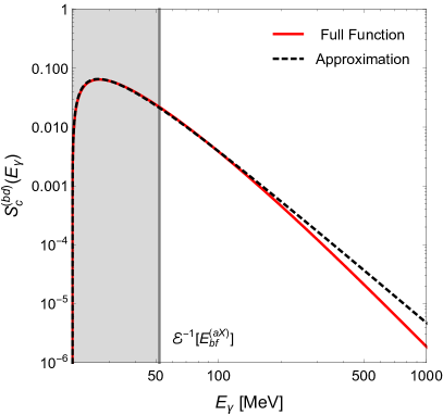
Figure 4: The exact value of the function $S_{c}^{(bd)}(E_{\gamma})$ for the process $\ce{{}^{4}He}+\gamma\rightarrow\ce{T}+p$ (red curve) and our approximation to this function in Eq. (45) (black dashed curve), plotted over the range $E_{c}^{(bd)}<E_{\gamma}\lower 3.01385pt\hbox{$\;\stackrel{{\scriptstyle\textstyle<}}{{\sim}}\;$}1$ GeV.  The gray vertical line corresponds to the minimum photon energy $\mathcal{E}^{-1}[E_{bf}^{(aX)}]$ for the production of an excited $\ce{T}$ nucleus above the kinetic-energy threshold for the secondary process $\ce{{}^{4}He}+\ce{T}\rightarrow\ce{{}^{6}Li}+n$. Thus, photons in the gray shaded region play no role in the secondary production of $\ce{{}^{6}Li}$. We note that the corresponding $S_{c}^{(bd)}(E_{\gamma})$ curves and thresholds for $\ce{{}^{4}He}+\gamma\rightarrow\ce{{}^{3}He}+n$ (the other primary process relevant for secondary $\ce{{}^{6}Li}$ production) are nearly identical to those shown here.

Armed with our approximation for $S_{c}^{(bd)}(E_{\gamma})$ in Eq. (45), it is now straightforward to evaluate the integral in Eq. (41) and obtain an approximate analytic expression for $\delta Y_{a}$. Just as it does for primary photoproduction and photodisintegration, the functional dependence of $\delta Y_{a}$ on $\tau_{\chi}$ for secondary production depends on the relationship between $\tau_{\chi}$ and a pair of characteristic timescales determined by the energy thresholds for the relevant processes. As we have discussed above, it is $\mathcal{E}^{-1}[E_{bf}^{(aX)}]$ rather than $E_{c}^{(bd)}$ which sets the minimum $E_{\gamma}$ required of a photon in order for it to contribute to the secondary production of $\ce{{}^{6}Li}$. It therefore follows that the characteristic timescales for the secondary production of this nucleus are determined by $\mathcal{E}^{-1}[E_{bf}^{(aX)}]$ rather than $E_{c}^{(bd)}$. Thus, for secondary production, we define

$$t_{Ca}^{(bcf)} \approx (10^{8}\,{\rm s})\times\left(\frac{\mathcal{E}^{-1}[E_{bf}^{(aX)}]}{103\,\,{\rm MeV}}\right)^{2}$$

$$t_{Xa}^{(bcf)} \approx (10^{8}\,{\rm s})\times\left(\frac{\mathcal{E}^{-1}[E_{bf}^{(aX)}]}{28\,\,{\rm MeV}}\right)^{2}~{}.$$ (46)

For $\tau_{\chi}<t_{Ca}^{(bcf)}$ within the uniform-decay approximation, $\delta Y_{a}$ is formally zero, as it is in the corresponding lifetime regime for primary production. Thus, in order to derive a meaningful constraint on unstable particles with lifetimes within this regime, we follow the same procedure as we employed in order to calculate the contribution to $\delta Y_{a}$ from primary production for a particle with $\tau_{\chi}<t_{Ca}^{(bc)}$. We model the injection of photons using the expression for secondary production appropriate for continuum injection, with $d\rho(t_{\mathrm{inj}})/dt_{\mathrm{inj}}$ given by Eq. (34). In analogy to our treatment of the primary process in this regime, we include only the contribution from injection times in the range $t_{Ca}^{(bcf)}<t_{\mathrm{inj}}<t_{Ca}^{(bcf)}+\tau_{\chi}$. Dropping terms beyond leading order in the dimensionless variable $w_{C\chi}\equiv\tau_{\chi}/t_{Ca}^{(bcf)}$, we find

$$\delta Y_{a}~{}=~{}\sum_{b,c,f}A_{a}^{(bcf)}\Omega_{\chi}w_{C\chi}e^{-w_{C\chi}^{-1}}~{},$$ (47)

where the proportionality constant $A_{a}^{(bcf)}$ for each combination of primary and secondary processes is independent of $\tau_{\chi}$. We note that the dependence of $\delta Y_{a}$ on $\tau_{\chi}$ in this expression is exactly the same as in Eq. (36). By contrast, for $t_{Ca}^{(bcf)}<\tau_{\chi}<t_{Xa}^{(bcf)}$, we find

$$\delta Y_{a} = \sum_{b,c,f}B_{a}^{(bcf)}\Omega_{\chi}\Bigg{[}(5-3\theta)-20\beta^{3}w_{X\chi}^{-3/2}$$ (48)

$$+15\beta^{4}(1+\theta)w_{X\chi}^{-2}\!\!-12\beta^{5}\theta w_{X\chi}^{-5/2}\Bigg{]}~{},~{}~{}~{}$$

where we have defined $w_{X\chi}\equiv\tau_{\chi}/t_{Xa}^{(bcf)}$ in analogy with $w_{C\chi}$ and where

$$\theta~{}\equiv~{}\frac{E_{c}^{(bd)}}{\mathcal{E}^{-1}\big{[}E_{bf}^{(aX)}\big{]}}$$ (49)

represents the ratio of the photon-energy threshold for primary production to the minimum photon energy needed to produce an excited nucleus of species $N_{b}$ with a kinetic energy above the energy threshold for the secondary process. Numerically, we find $\theta\approx 0.46$ for $\ce{{}^{4}He}+\gamma\rightarrow\ce{T}+p$ followed by $\ce{{}^{4}He}+\ce{T}\rightarrow\ce{{}^{6}Li}+n$, while $\theta\approx 0.52$ for $\ce{{}^{4}He}+\gamma\rightarrow\ce{{}^{3}He}+n$ followed by $\ce{{}^{4}He}+\ce{{}^{3}He}\rightarrow\ce{{}^{6}Li}+p$. Finally, for $t_{Xa}^{(bcf)}<\tau_{\chi}$, we find

$$\delta Y_{a} = \sum_{b,c,f}B_{a}^{(bcf)}\Omega_{\chi}\Bigg{[}\frac{16}{21}(9-5\theta)w_{X\chi}^{-1/4}\!\!$$ (50)

$$-4(1+5\beta^{3})w_{X\chi}^{-3/2}+\frac{15}{7}(1+\theta)(1+7\beta^{4})w_{X\chi}^{-2}$$

$$-\frac{4}{3}\theta(1+9\beta^{5})w_{X\chi}^{-5/2}\Bigg{]}~{}.$$

Thus, to summarize, we have derived a set of simple, analytic approximations for the change $\delta Y_{a}$ in the abundance of a given nuclear species $N_{a}$ due to the late injection of photons by a decaying particle $\chi$. For primary photoproduction or photodisintegration processes, we find that $\delta Y_{a}$ is given by Eq. (36), Eq. (37), or Eq. (38), depending on the lifetime $\tau_{\chi}$ of the particle. Likewise, for secondary production, we find that $\delta Y_{a}$ is given by Eq. (47), Eq. (48), or Eq. (50) within the corresponding lifetime regimes.

III.7 The Fruits of Linearization:  Light-Element Constraints on Ensembles of Unstable Particles

We now turn to the task of extending these results to the case of an ensemble of decaying particles $\chi_{i}$ with lifetimes $\tau_{i}$ and extrapolated abundances $\Omega_{i}$. Indeed, we have seen that if the linearity criterion is satisfied both for $N_{a}$ itself and for all of its source nuclei $N_{b}\neq N_{a}$, all feedback effects on $Y_{a}$ can be neglected. Thus, in this regime, the overall change $\delta Y_{a}$ in the abundance of a light nucleus is well approximated by the sum of the individual contributions associated with the individual $\chi_{i}$ from each pertinent process. Indeed, it is only because we have entered a linear regime that such a direct sum is now appropriate. These, then, are the fruits of linearization.

While certain nuclei in our analysis — namely $\ce{{}^{6}Li}$ and $\ce{{}^{7}Li}$ — do not have the property that the linearity criterion is always satisfied for both the nucleus itself and its source nuclei, we emphasize that we are nevertheless able to derive meaningful bounds on the comoving number densities of these nuclei. As noted in Sect. III.4, artificially adopting the linearity criterion for $Y_{\ce{{}^{7}Li}}$ in the Boltzmann equation for $\ce{{}^{6}Li}$ always yields a conservative bound on $\delta Y_{\ce{{}^{6}Li}}$, regardless of the injection history. For $\ce{{}^{7}Li}$, the issue is that feedback effects on the photodisintegration rate due to changes in the comoving number density of $\ce{{}^{7}Li}$ itself are not necessarily small. Thus, strictly speaking, $\delta Y_{\ce{{}^{7}Li}}$ is not well approximated by a direct sum of the contributions from the individual $\chi_{i}$. However, since this direct sum is simply an approximation of the integral in Eq. (25), it is equivalent to the quantity $Y_{\ce{{}^{7}Li}}^{\mathrm{init}}\ln[1+\delta Y_{\ce{{}^{7}Li}}(t)/Y_{\ce{{}^{7}Li}}^{\mathrm{init}}]$. Thus, for all relevant $N_{a}$, we find that an ensemble of decaying particles makes an overall contribution to $\delta Y_{a}$ — or, in the case of $\ce{{}^{7}Li}$, to the quantity $Y_{a}^{\mathrm{init}}\ln[1+\delta Y_{a}(t)/Y_{a}^{\mathrm{init}}]$ — which can be approximated as a direct sum of the individual contributions from the individual ensemble constituents. Indeed, this yields either a reliable estimate for the true value of $\delta Y_{a}$ or a reliably conservative bound on $\delta Y_{a}$.

In principle, each of these individual contributions to a given $\delta Y_{a}$ can involve a large number of reactions with different energy thresholds and scattering kinematics, each with its own distinct fit parameters $A_{a}^{(bc)}$, $B_{a}^{(bc)}$, $t_{Xa}^{(bc)}$, $t_{Ca}^{(bc)}$, etc.  In practice, however, the number of reactions which contribute significantly to $\delta Y_{a}$ for any one of the four relevant nuclear species is quite small, as can be seen from Table 1.  Moreover, it is often the case that many if not all of the reactions which have a non-negligible impact on a given $\delta Y_{a}$ have very similar energy thresholds and scattering kinematics. When this is the case, the contribution to $\delta Y_{a}$ from these processes can, to a very good approximation, collectively be modeled using a single set of fit parameters. For example, the only reactions which have a significant impact on $\delta Y_{\ce{{}^{4}He}}$ are the primary photodisintegration processes $\ce{{}^{4}He}+\gamma\rightarrow\ce{T}+p$ and $\ce{{}^{4}He}+\gamma\rightarrow\ce{{}^{3}He}+n$, which have very similar energy thresholds and scattering kinematics. Thus, a fit involving a single set of parameters yields an accurate approximation for $\delta Y_{\ce{{}^{4}He}}$. The reactions which contribute to $\delta Y_{\ce{{}^{7}Li}}$ differ more significantly in terms of their energy thresholds and scattering kinematics. Nevertheless, as we shall see, the collective effect of these processes is also well modeled by a single set of fit parameters. By contrast, for $\ce{D}$ there are two processes with qualitatively different energy thresholds and scattering kinematics which must be modeled using separate sets of fit parameters: primary photodisintegration via $\ce{D}+\gamma\rightarrow n+p$ and primary photoproduction via $\ce{{}^{4}He}+\gamma\rightarrow\ce{D}+n+p$. Likewise, for $\ce{{}^{6}Li}$, two sets of fit parameters are required: one for primary photoproduction via $\ce{{}^{7}Li}+\gamma\rightarrow\ce{{}^{6}Li}+n$ and one for secondary production via both $\ce{{}^{4}He}+\ce{{}^{3}He}\rightarrow\ce{{}^{6}Li}+p$ and $\ce{{}^{4}He}+\ce{T}\rightarrow\ce{{}^{6}Li}+n$.

Nucleus	Process	$t_{Ba}(s)$	$t_{Ca}(s)$	$t_{Xa}(s)$	$A_{a}$	$B_{a}$	$\delta Y_{a}^{\mathrm{min}}$	$\delta Y_{a}^{\mathrm{max}}$
^4He	Destruction	$~{}8.9\times 10^{6}$	$~{}3.2\times 10^{6}$	$~{}4.2\times 10^{7}~{}$	$-3.3\times 10^{-1}$	$-1.5\times 10^{0}$	$-3.0\times 10^{-3}$	—
^7Li	Destruction	$4.5\times 10^{5}$	$5.7\times 10^{4}$	$1.6\times 10^{6}$	$-2.7\times 10^{-10}~{}$	$-3.8\times 10^{-9}$	$-5.5\times 10^{-11}$	—
D	Destruction	$2.2\times 10^{5}$	$4.6\times 10^{4}$	$1.1\times 10^{6}$	$-1.2\times 10^{-4}$	$-1.2\times 10^{-3}$	$-8.9\times 10^{-7}$	$1.6\times 10^{-6}$
	Production*	$1.9\times 10^{7}$	$8.0\times 10^{6}$	$1.1\times 10^{8}$	$1.8\times 10^{-2}$	$8.2\times 10^{-2}$
^6Li	Primary Production	$1.8\times 10^{6}$	$6.0\times 10^{5}$	$1.0\times 10^{7}$	$1.6\times 10^{-10}$	$9.8\times 10^{-10}$	—	$1.8\times 10^{-11}$
	Secondary Production*	$8.9\times 10^{7}$	$1.9\times 10^{7}$	$4.6\times 10^{8}$	$8.0\times 10^{-8}$	$1.8\times 10^{-7}$

Table 2:  Values for the fit parameters appearing in Eqs. (LABEL:eq:BBNFitsTerm1)–(LABEL:eq:BBNFitsLi6) which characterize the contribution to the change $\delta Y_{a}$ in the comoving number density of nucleus $N_{a}$ due to the electromagnetic decays of unstable particles after BBN.  An asterisk appearing after the name of the process indicates that the values listed in the table correspond to the parameters $A_{a}^{\ast}$, $B_{a}^{\ast}$, $t_{Ca}^{\ast}$, $t_{Xa}^{\ast}$, etc., associated with $\delta Y_{a}^{(2)}$ for the nucleus in question rather than the parameters $A_{a}$, $B_{a}$, $t_{Ca}$, $t_{Xa}$, etc., associated with $\delta Y_{a}^{(1)}$. The observational upper and lower limits $\delta Y_{a}^{\mathrm{min}}$ and $\delta Y_{a}^{\mathrm{max}}$ on the value of $\delta Y_{a}$ are also shown.

In general, then, we require at most two distinct sets of parameters in order to model the overall contribution to $\delta Y_{a}$ for each relevant nucleus due to electromagnetic injection from an ensemble of decaying particles. Thus, in general, we may express this overall contribution as the sum of two terms

$$\delta Y_{a}~{}=~{}\delta Y_{a}^{(1)}+\delta Y_{a}^{(2)}~{}.$$ (51)

For each relevant nuclear species, one of these terms is associated with a primary process: primary photoproduction in the case of $\ce{{}^{6}Li}$ and primary photodisintegration in the case of $\ce{{}^{4}He}$, $\ce{{}^{7}Li}$, and $\ce{D}$. Thus, $\delta Y_{a}^{(1)}$ takes a universal form for all relevant nuclear species. In particular, Eqs. (47)–(50) suggest that we may model $\delta Y_{a}^{(1)}$ with a function of the form

$$\delta Y_{a}^{(1)} = \!\!\!\!\!\!\!\sum_{t_{Aa}<\tau_{i}<t_{Ba}}\!\!\!\!\!\!\!\!A_{a}\Omega_{i}\left(\frac{\tau_{i}}{t_{Ca}}\right)e^{-t_{Ca}/\tau_{i}}$$

$$+ \!\!\!\!\!\!\!\sum_{t_{Ba}<\tau_{i}<t_{Xa}}\!\!\!\!\!B_{a}\Omega_{i}\left[1-\beta\left(\frac{t_{Xa}}{\tau_{i}}\right)^{\!1/2}\right]$$

$$+ \!\!\!\!\!\!\!\sum_{t_{Xa}<\tau_{i}<t_{fa}}\!\!\!\!\!\!\!\!B_{a}\Omega_{i}\left(\frac{t_{Xa}}{\tau_{i}}\right)^{\!1/4}\!\left[2-(1+\beta)\left(\frac{t_{Xa}}{\tau_{i}}\right)^{\!1/4}\right]~{},$$

where $A_{a}$, $B_{a}$, $t_{Ca}$, $t_{Xa}$, etc., are model parameters whose assignments we shall discuss below. By contrast, the form of the second term in Eq. (51) differs depending on the nucleus in question. For $\ce{{}^{4}He}$ and $\ce{{}^{7}Li}$, we simply have $\delta Y_{a}^{(2)}=0$. For $\ce{D}$, this term is associated with primary production and thus takes exactly the same functional form as $\delta Y_{a}^{(1)}$. In other words, we have

$$\delta Y_{a}^{(2)} = \!\!\!\!\!\!\!\!\sum_{t_{Aa}^{*}<\tau_{i}<t_{Ba}^{*}}\!\!\!\!\!\!\!\!\!A_{a}^{*}\Omega_{i}\left(\frac{\tau_{i}}{t_{Ca}^{*}}\right)e^{-t_{Ca}^{*}/\tau_{i}}$$

$$\,+ \!\!\!\!\!\sum_{t_{Ba}^{*}<\tau_{i}<t_{Xa}^{*}}\!\!\!\!\!\!\!\!\!B_{a}^{*}\Omega_{i}\left[1-\beta\left(\frac{t_{Xa}^{*}}{\tau_{i}}\right)^{\!1/2}\right]$$

$$\,+ \!\!\!\!\!\sum_{t_{Xa}^{*}<\tau_{i}<t_{fa}^{*}}\!\!\!\!\!\!\!\!\!B_{a}^{*}\Omega_{i}\left(\frac{t_{Xa}^{*}}{\tau_{i}}\right)^{\!1/4}\!\left[2-(1+\beta)\left(\frac{t_{Xa}^{*}}{\tau_{i}}\right)^{\!1/4}\right]~{},$$

where $A_{a}^{\ast}$, $B_{a}^{\ast}$, $t_{Ca}^{\ast}$, $t_{Xa}^{\ast}$, etc., represent an additional set of model parameters distinct from the parameters $A_{a}$, $B_{a}$, $t_{Ca}$, $t_{Xa}$, etc., in Eq. (LABEL:eq:BBNFitsTerm1). For $\ce{{}^{6}Li}$, the term $\delta Y_{a}^{(2)}$ is associated with secondary production and therefore takes the form

$$\delta Y_{a}^{(2)} = \!\!\!\!\!\!\!\!\sum_{t_{Aa}^{*}<\tau_{i}<t_{Ba}^{*}}\!\!\!\!\!\!\!\!\!A_{a}^{*}\Omega_{i}\left(\!\frac{\tau_{i}}{t_{Ca}^{*}}\!\right)e^{-t_{Ca}^{*}/\tau_{i}}$$

$$\,+ \!\!\!\!\!\!\!\!\sum_{t_{Ba}^{*}<\tau_{i}<t_{Xa}^{*}}\!\!\!\!\!\!\!\!\!B_{a}^{*}\Omega_{i}\Bigg{[}(5-3\theta)-20\beta^{3}\left(\!\frac{t_{Xa}^{*}}{\tau_{i}}\!\right)^{\!3/2}\!\!\!\!+15\beta^{4}(1+\theta)\left(\!\frac{t_{Xa}^{*}}{\tau_{i}}\!\right)^{\!2}\!\!-12\beta^{5}\theta\left(\!\frac{t_{Xa}^{*}}{\tau_{i}}\!\right)^{\!5/2}\Bigg{]}$$

$$\,+ \!\!\!\!\!\!\!\!\sum_{t_{Xa}^{*}<\tau_{i}<t_{fa}^{*}}\!\!\!\!\!\!\!\!\!B_{a}^{*}\Omega_{i}\Bigg{[}\frac{16}{21}(9-5\theta)\left(\!\frac{t_{Xa}^{*}}{\tau_{i}}\!\right)^{\!1/4}\!\!\!\!-4(1+5\beta^{3})\left(\!\frac{t_{Xa}^{*}}{\tau_{i}}\!\right)^{\!3/2}\!\!\!\!+\frac{15}{7}(1+\theta)(1+7\beta^{4})\left(\!\frac{t_{Xa}^{*}}{\tau_{i}}\!\right)^{\!2}\!\!-\frac{4}{3}\theta(1+9\beta^{5})\left(\!\frac{t_{Xa}^{*}}{\tau_{i}}\!\right)^{\!5/2}\Bigg{]}~{}.$$

We note that for simplicity and compactness of notation, we have implicitly taken $\epsilon_{i}=1$ for each $\chi_{i}$ in formulating the expressions appearing in Eqs. (LABEL:eq:BBNFitsTerm1)–(LABEL:eq:BBNFitsLi6). However, it is straightforward to generalize these results to the case in which $\epsilon_{i}$ differs from unity for one or more of the $\chi_{i}$. In particular, the corresponding expressions for $\delta Y_{a}^{(1)}$ and $\delta Y_{a}^{(2)}$ in this case may be obtained by replacing $\Omega_{i}$ for each species with the product $\Omega_{i}\epsilon_{i}$. Moreover, we remind the reader that for the case of $\ce{{}^{7}Li}$, a more accurate estimate of $\delta Y_{a}$ can be obtained by replacing $\delta Y_{a}^{(1)}$ with $Y_{a}^{\mathrm{init}}\ln[1+\delta Y_{a}^{(1)}(t)/Y_{a}^{\mathrm{init}}]$ in Eq. (LABEL:eq:BBNFitsTerm1).

We now determine the values of the parameters in Eq. (LABEL:eq:BBNFitsTerm1). We begin by noting that the parameter $t_{Aa}$ for each relevant nucleus $N_{a}$ may be assigned essentially any value between the end of the BBN epoch and the timescale at which the first reaction which contributes to $\delta Y_{a}$ becomes efficient. Thus, for simplicity, we choose a universal value $t_{Aa}=10^{4}$ s for all $N_{a}$, which corresponds to the timescale at which the first reaction in Table 1 — namely the photodisintegration process $\ce{D}+\gamma\rightarrow n+p$ — effectively turns on. For $t_{fa}$, we likewise choose a universal value $t_{fa}=10^{12}$ s for all $N_{a}$. As discussed in Sect. VI, the reason for this choice is that many of the Class-I processes which serve to establish the reprocessed photon spectrum in Eq. (1) start to become inefficient around this timescale. As a result, the photon spectrum that results from electromagnetic injection at times $t_{\mathrm{inj}}\gtrsim 10^{12}$ s differs from that in Eq. (1), and the analytic approximation for $\delta Y_{a}^{(1)}$ in Eq. (LABEL:eq:BBNFitsTerm1) is no longer reliable. The values of $t_{Aa}^{\ast}$ and $t_{fa}^{\ast}$ appearing in Eqs. (LABEL:eq:BBNFitsTerm2) and (LABEL:eq:BBNFitsLi6) are determined in the same way.

Given these results, we now determine the values of the remaining parameters in Eqs. (LABEL:eq:BBNFitsTerm1)–(LABEL:eq:BBNFitsLi6) by demanding that the constraint contour we obtain from each of these equations be consistent with the contour obtained from a more complete numerical analysis of the Boltzmann system in the limiting case in which our decaying “ensemble” comprises only a single particle species $\chi$. In this single-particle case, our analytic expression for $\delta Y_{a}$ becomes a function of only two variables: the abundance $\Omega_{\chi}$ and lifetime $\tau_{\chi}$ of $\chi$. We determine the constraint contours corresponding to the observational limits quoted in Sect. III.3 by surveying ($\Omega_{\chi}$,$\tau_{\chi}$) space and numerically solving the full, coupled system of Boltzmann equations for $\delta Y_{a}$ at each point. The undetermined parameters in Eqs. (LABEL:eq:BBNFitsTerm1)–(LABEL:eq:BBNFitsLi6) are then chosen such that our analytic expression provides a good fit to the corresponding constraint contour for each nucleus. We list the values for all parameters obtained in this manner in Table 2.

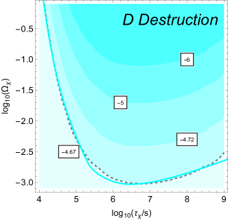
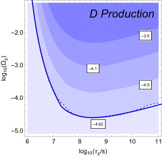
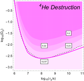
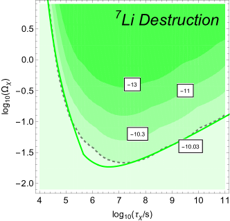
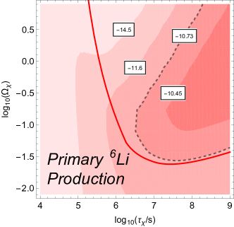
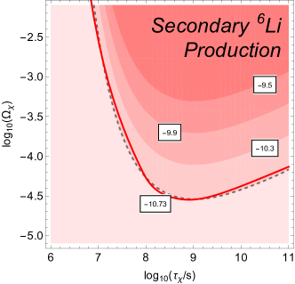
Figure 5: Numerical results for $\delta Y_{a}$ for each relevant nucleus in the presence of a single electromagnetically-decaying particle $\chi$ with extrapolated abundance $\Omega_{\chi}$ and lifetime $\tau_{\chi}$. In all panels except that pertaining to $\ce{{}^{4}He}$ destruction, we plot contours of $\log_{10}Y_{a}$, while for $\ce{{}^{4}He}$ destruction we plot contours of $Y_{p}$. Note that for later reference, we have plotted separate contours for $\ce{D}$ production and destruction; likewise, we show separate contours for primary and secondary $\ce{{}^{6}Li}$ production. Regions of the $(\tau_{\chi},\Omega_{\chi})$ plane which are found by numerical analysis to be excluded are those above and/or to the right of the gray dashed line in each panel, while the solid colored curve in each panel demarcates the analogous region found to be excluded by fitting the free parameters in our analytic approximations for $\delta Y_{a}$ in Eqs. (LABEL:eq:BBNFitsTerm1)–(LABEL:eq:BBNFitsLi6) to our numerical results. We see that the full numerical results and our analytic approximations agree very well in all cases except that of primary $\ce{{}^{6}Li}$ production, where our analytic approximation diverges from the numerical result at large $\Omega_{\chi}$ and thus provides an even more conservative bound on the allowed parameter space.

In deriving these constraint contours, it is necessary to translate the observational constraints in Eqs. (18)–(21) on the relevant $Y_{a}$ at the end of the BBN epoch into bounds of the form

$$\delta Y_{a}^{\mathrm{min}}~{}<~{}\delta Y_{a}~{}<~{}\delta Y_{a}^{\mathrm{max}}$$ (55)

on the corresponding subsequent change $\delta Y_{a}$ in each $Y_{a}$. In so doing, we must specify a set of initial values of $Y_{a}$ at the end of BBN.  For $Y_{\ce{{}^{4}He}}$ and $Y_{\ce{{}^{7}Li}}$, we take $Y_{p}=0.2449$ and $\ce{{}^{7}Li}/\ce{H}=1.6\times 10^{-10}$, as discussed in Sect. III.4. For $Y_{\ce{D}}$, we take the value which corresponds to the central theoretical prediction $\ce{D}/\ce{H}=2.413\times 10^{-5}$ for the primordial $\ce{D}/\ce{H}$ ratio derived in Ref. CookeDUpper . Finally, since $\ce{{}^{6}Li}$ is not produced in any significant amount during BBN, we take $Y_{\ce{{}^{6}Li}}=0$. The values for the observational upper and lower limits $\delta Y_{a}^{\mathrm{min}}$ and $\delta Y_{a}^{\mathrm{max}}$ on $\delta Y_{a}$ which correspond to these choices for the initial $Y_{a}$ are listed in Table 2 alongside the values for our fit parameters.

In Fig. 5, we display contours showing the results of our numerical calculation of $\delta Y_{a}$ in $(\Omega_{\chi},\tau_{\chi})$ space for each relevant nucleus. More specifically, we display contours of $Y_{p}$ for $\ce{{}^{4}He}$, whereas we display contours of $\log_{10}Y_{a}$ for $\ce{D}$, $\ce{{}^{7}Li}$, and $\ce{{}^{6}Li}$. Moreover, for purposes of illustration, we display separate contours for $\ce{D}$ production and destruction — i.e., contours evaluated considering either production or destruction processes in $\mathcal{C}_{\ce{D}}^{(p)}$ only, with the cross-sections for the opposite set of processes artificially set to zero. Likewise, we also display separate contours for primary and secondary $\ce{{}^{6}Li}$ production. We emphasize, however, that in assessing our overall constraints on decaying ensembles, we consider these processes together, allowing for the possibility of a cancellation between the two individual contributions to $\delta Y_{a}$ (in the case of $\ce{D}$) or a reinforcement (in the case of $\ce{{}^{6}Li}$). The gray dashed line in each panel of Fig. 5 indicates the upper bound on $\Omega_{\chi}$ obtained through a numerical calculation of $\delta Y_{a}$ which follows from the observational limits in Eqs. (18)–(21). By contrast, the solid curve in each panel represents the corresponding constraint contour obtained through our analytic approximation for $\delta Y_{a}$ in Eq. (51).

We see from Fig. 5 that in all cases except for that of primary $\ce{{}^{6}Li}$ production, the constraint contours we obtain using the linear and uniform-decay approximations are quite similar to those obtained in the more realistic case in which we account for the fact that $\chi$ has a constant decay rate and in which we account for feedback effects in the collision terms $\mathcal{C}_{a}^{(p)}$ and $\mathcal{C}_{a}^{(s)}$ for each relevant nucleus. Moreover, as discussed in Sect. III.4, we see that for primary $\ce{{}^{6}Li}$ production the constraint contour obtained using these approximations indeed represents a conservative bound on $\Omega_{\chi}$. We also note that with this sole exception, the results of our analytic approximations are in good agreement with the corresponding results in Ref. CyburtEllisUpdated within the regime in which $\Omega_{\chi}$ is small and the linear approximation holds. Once again, we note that the effects of additional processes which we do not incorporate into this analysis can have important effects on the $Y_{a}$ in the regime in which $\Omega_{\chi}$ — and therefore the overall magnitude of electromagnetic injection — is large. These include, for example, photodisintegration processes which contribute to the depletion of a previously generated population of $\ce{{}^{6}Li}$ as well as additional processes which contribute to the production or destruction of $\ce{D}$ CyburtEllisUpdated . However, since the regions of $(\Omega_{\chi},\tau_{\chi})$ space in which these effects on $\ce{D}$ and $\ce{{}^{6}Li}$ are relevant are excluded by constraints on the primordial abundances of other nuclei, our neglecting these processes will have essentially no impact on the overall constraints we derive on ensembles of decaying particles.

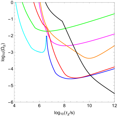
Figure 6: Compilation of constraints on electromagnetic injection from bounds on the abundances of light nuclei. The individual contours shown indicate the constraints stemming from considerations of $\ce{D}$ production (dark blue) and destruction (light blue), $\ce{{}^{7}Li}$ destruction (green), $\ce{{}^{4}He}$ destruction (magenta), and $\ce{{}^{6}Li}$ production (red), the latter including both primary and secondary contributions. In addition, we also plot constraints stemming from limits on potential distortions of the CMB-photon spectrum, both $\mu$-type (orange) and $y$-type (black), as will be discussed in Sect. IV.  In each case, the regions of parameter space above each contour are excluded.

In Fig. 6 we plot our analytic approximations to the constraint contours obtained for each relevant nucleus together in $(\Omega_{\chi},\tau_{\chi})$ space. Note that the $\ce{{}^{6}Li}$ contour includes both primary and secondary contributions to $\delta Y_{\ce{{}^{6}Li}}$. In determining the $\ce{D}$ contour, we have included contributions from both photoproduction and photodisintegration processes, the interference between which is responsible for the “funnel” region at $\tau_{\chi}\approx 10^{6.5}$ s within which the bound on $\Omega_{\chi}$ is considerably weakened. However, since the upper and lower bounds on $\delta Y_{\ce{D}}$ derive from different considerations, different colors are used to distinguish the part of the contour which corresponds to the upper bound (dark blue) from the part which corresponds to the lower bound (light blue). We note that in all cases, these contours are in good agreement with the corresponding results in Ref. CyburtEllisUpdated within the regime in which $\Omega_{\chi}$ is small and the linear approximation holds.

IV Spectral Distortions in the CMB

In addition to altering the abundances of light nuclei, electromagnetic injection from the decays of unstable particles in the early universe can also have observable effects on the spectrum of CMB photons, distorting that spectrum away from a pure blackbody profile. Observational limits on these distortions therefore also constrain such decays. Once again, while the constraints on a single decaying particle species are well known, the corresponding constraints on an ensemble of decaying particles are less well established. Our aim in this section is to derive approximate analytic expressions for the CMB distortions which can arise due to entire ensembles of decaying particles — expressions analogous to those we derived in Sect. III for the change $\delta Y_{a}$ in the comoving number density in each relevant nucleus after BBN.

One of the subtleties which arises in constraining distortions in the CMB-photon spectrum from ensembles of decaying particles with a broad range of lifetimes is that both the manner in which that spectrum is distorted and the magnitude of that distortion depend on the timescale over which the injection takes place. At early times, energetic photons produced by these decays are rapidly brought into both kinetic and thermal equilibrium by the Class-III processes discussed in Sect. II. As a result, the spectrum of photons retains a blackbody shape. However, at later times, photon-number-changing processes such as double-Compton scattering and bremsstrahlung “freeze out,” in the sense that the rates for these processes drop below the expansion rate $H$ of the universe. Once this occurs, injected photons are no longer able to attain thermal equilibrium with photons in the radiation bath. Nevertheless, they are able to attain kinetic equilibrium with these photons through elastic Compton scattering. As a result, the photon spectrum no longer retains its original blackbody shape; rather, it is distorted into a Bose-Einstein distribution characterized by a pseudo-degeneracy parameter $\mu$.

Eventually, at an even later time $t_{\mathrm{EC}}\approx 9\times 10^{9}~{}\rm s$, elastic Compton scattering also freezes out. Thus, photons injected at times $t\gtrsim t_{\mathrm{EC}}$ attain neither kinetic nor thermal equilibrium with photons in the radiation bath. Nevertheless, the injected photons continue to interact with electrons in the radiation bath at an appreciable rate until the time of last scattering $t_{\mathrm{LS}}\approx 1.19\times 10^{13}$ s. During this window, photons in the radiation bath are up-scattered by electrons which acquire significant energy from these interactions. The ultimate result is a photon spectrum which is suppressed at low frequencies and enhanced at high frequencies. This spectral distortion is characterized by a non-zero Compton $y$ parameter $y_{C}$. Finally, after last scattering, any additional photons injected from particle decay simply contribute to the diffuse photon background.

In order to derive analytic expressions for the constraints on the parameters $\mu$ and $y_{C}$ in the presence of a decaying ensemble, we shall once again make use of the uniform-decay approximation as well as a linear approximation similar to the approximation we invoked in calculating the $\delta Y_{a}$ in Sect. III.  The validity of such an approximation follows from the fact that both $\mu$ and $y_{C}$ are tightly constrained by observation. The most stringent limits on these parameters, which are currently those from COBE/FIRAS data COBEFIRAS , are

$$|\mu| < 9.0\times 10^{-5}$$

$$y_{C} < 1.2\times 10^{-5}~{}.$$ (56)

Moreover, proposed broad-spectrum experiments, such as PIXIE PIXIE , could potentially increase the sensitivity to which these distortions can be probed by more than an order of magnitude. These stringent constraints on the shape of the CMB-photon spectrum imply that the contribution $\delta\rho_{\gamma}$ to the photon energy density from injection during the relevant epoch must be quite small, in the sense that $\delta\rho_{\gamma}\ll\rho_{\gamma}$. Thus, to a very good approximation, we may ignore feedback effects on the overall photon number density $n_{\gamma}$ and energy density $\rho_{\gamma}$ when analyzing distortions in that spectrum. This allows us to replace these quantities by their equilibrium values.

This linear approximation significantly simplifies the analysis of the resulting CMB spectrum HuAndSilk ; HuAndSilk2 ; ChlubaSunyaev ; BeyondYAndMu . For example, in this approximation we may study the evolution of the CMB-photon spectrum using the method of Green’s functions ChlubaGreensFns1 ; BeyondYAndMu ; ChlubaGreensFns2 . In this approach, we may express a generic spectral distortion which constitutes a shift $\Delta I_{\nu}(t_{\mathrm{now}})$ in the present-day intensity of photons with frequency $\nu$ relative to the expected intensity in the standard cosmology in the form

$$\Delta I_{\nu}(t_{\mathrm{now}})~{}=~{}\int G(\nu,t,t_{\mathrm{now}})\,\frac{d}{dt}\left(\frac{Q}{\rho_{\gamma}}\right)dt~{},$$ (57)

where $Q$ is the energy density injected at time $t$ and where $G(\nu,t,t^{\prime})$ is a Green’s function which relates the intensity of photons with frequency $\nu$ injected at time $t$ to the photon intensity at that same frequency at a later time $t^{\prime}>t$. In general, $G(\nu,t,t_{\mathrm{now}})$ is well approximated by a sum of terms representing an overall temperature shift, a $\mu$-type distortion, and $y$-type distortion ChlubaGreensFns1 . This Green’s-function formalism provides a tool for numerically estimating the overall distortion to the CMB-photon spectrum from any arbitrary injection history, provided that the overall injected energy is small. We shall draw on this formalism extensively in deriving our analytic approximations for $\delta\mu$ and $\delta y_{C}$.

IV.1 The $\mu$ Parameter

The time-evolution of the pseudo-degeneracy parameter $\mu$ is governed by an equation of the form HuAndSilk ; HuAndSilk2

$$\frac{d\mu}{dt}~{}=~{}\frac{d\mu_{\mathrm{inj}}}{dt}-\mu(\Gamma_{\mathrm{DC}}+\Gamma_{\mathrm{BR}})~{}.$$ (58)

The first term in Eq. (58) is a source term which arises due to the injection of energetic photons. Within the linear approximation, this source term takes the generic form

$$\frac{d\mu_{\mathrm{inj}}}{dt}~{}\approx~{}\frac{1}{2.143}\left[\frac{3}{\rho_{\gamma}}\frac{d\rho_{\gamma}}{dt}-\frac{4}{n_{\gamma}}\frac{dn_{\gamma}}{dt}\right]~{},$$ (59)

where $n_{\gamma}$ and $\rho_{\gamma}$ respectively denote the overall number density and energy density of photons. We emphasize that this expression is completely general and applies even in absence of any source of photon injection, in which case the two terms in Eq. (59) cancel.

The second term in Eq. (58) is a sink term associated with processes which serve to bring the population of photons in the radiation bath into thermal equilibrium and thereby erase $\mu$. As discussed above, the dominant such processes are double-Compton scattering and bremsstrahlung, the respective thermalization rates for which are well approximated by power-law expressions of the form HuAndSilk

$$\Gamma_{\mathrm{DC}} = \Gamma_{\mathrm{DC}}^{\mathrm{MRE}}\left(\frac{t}{t_{\mathrm{MRE}}}\right)^{-9/4}$$

$$\Gamma_{\mathrm{BR}} = \Gamma_{\mathrm{BR}}^{\mathrm{MRE}}\left(\frac{t}{t_{\mathrm{MRE}}}\right)^{-13/8}~{},$$ (60)

where $t_{\mathrm{MRE}}$ once again denotes the time of matter-radiation equality. The coefficients in this expression are given by

$$\Gamma_{\mathrm{DC}}^{\mathrm{MRE}} \approx \left(5.73\times 10^{-39}\,{\rm GeV}\right)\left(\Omega_{B}h^{2}\right)$$

$$\times\left(1-\frac{Y_{p}}{2}\right)\left(\frac{T_{\mathrm{now}}}{2.7\mbox{~{}K}}\right)^{3/2}$$

$$\Gamma_{\mathrm{BR}}^{\mathrm{MRE}}~{} \approx \left(1.57\times 10^{-36}\,{\rm GeV}\right)\left(\Omega_{B}h^{2}\right)^{3/2}$$ (61)

$$\times\left(1-\frac{Y_{p}}{2}\right)\left(\frac{T_{\mathrm{now}}}{2.7\mbox{~{}K}}\right)^{-5/4}~{},~{}~{}~{}$$

where $h$ is the Hubble constant, $\Omega_{B}$ is the present-day abundance of baryons, and $T_{\mathrm{now}}\approx 2.7$ K is the present-day temperature of the CMB. For completeness, we note that the expression for $\Gamma_{\mathrm{BR}}$ in Eq. (60) represents an overestimate of the true bremsstrahlung rate. In particular, a full frequency-dependent treatment of the evolution of the photon spectrum reveals that bremsstrahlung is less efficient at early times KhatriSunyaev . As a result, the true bremsstrahlung rate is actually smaller than the result in Eq. (60) would suggest. However, we shall find below that the effect of bremsstrahlung on $\mu$ is subleading in comparison to the effect of double-Compton scattering, even with our overestimate for $\Gamma_{\mathrm{BR}}$. Given this, we shall choose to ignore the effect of bremsstrahlung entirely at a later stage of our analysis. Thus, our use of the expression in Eq. (60) for the bremsstrahlung rate will ultimately have no effect on our overall results.

Up to this point, our expressions governing the evolution of $\mu$ are completely general and may be applied to any injection history, provided that the total energy density injected is sufficiently small that the linear approximation is valid. In order to derive an approximate analytic expression for the overall change $\delta\mu$ in $\mu$ due to an ensemble of unstable particles, we proceed in essentially the same manner as we did in deriving expressions for the changes $\delta Y_{a}$ in the comoving number densities of light nuclei in Sect. III.  We begin by deriving an expression for $\delta\mu$ in the presence of a single decaying particle species $\chi$ with mass $m_{\chi}$ and lifetime $\tau_{\chi}$. When we take into account the full exponential nature of the decay, we find

$$\frac{d\rho_{\gamma}}{dt} = -4H\rho_{\gamma}+\epsilon_{\chi}\Gamma_{\chi}\rho_{\chi}$$

$$\frac{dn_{\gamma}}{dt} = -3Hn_{\gamma}+\frac{N_{\chi}^{(\gamma)}\Gamma_{\chi}\rho_{\chi}}{m_{\chi}}~{},$$ (62)

where $N_{\chi}^{(\gamma)}$ is the average number of photons produced per decay and where $\epsilon_{\chi}$ is the fraction of the energy released by $\chi$ decays which is transferred to photons. By contrast, within the uniform-decay approximation in which $d\rho_{\chi}/dt$ is given by Eq. (10), we have

$$\frac{d\rho_{\gamma}}{dt} = -4H\rho_{\gamma}+\epsilon_{\chi}\rho_{\chi}(\tau_{\chi})\delta(\tau_{\chi}-t)$$

$$\frac{dn_{\gamma}}{dt} = -3Hn_{\gamma}+\frac{N_{\chi}^{(\gamma)}\rho_{\chi}(\tau_{\chi})}{m_{\chi}}\delta(\tau_{\chi}-t)~{}.$$ (63)

In this approximation, a simple, analytic expression for $\delta\mu$ may be obtained by directly integrating Eq. (58) from the time $t_{e}\approx 1.69\times 10^{3}~{}\rm s$ at which electron-positron annihilation freezes out to the time $t_{\mathrm{EC}}$ at which elastic Compton scattering freezes out. In particular, we find that a particle species with a lifetime $\tau_{\chi}$ anywhere within this range gives rise to a $\mu$-type distortion of size

$$\delta\mu \approx \frac{\eta}{2.143}\left[\frac{90\zeta(3)\epsilon_{\chi}}{\pi^{4}}\left(\frac{\tau_{\chi}}{\rm s}\right)^{1/2}\!\!\!-4N_{\chi}^{(\gamma)}\left(\frac{m_{\chi}}{\,{\rm MeV}}\right)^{-1}\right]$$ (64)

$$\times\left(\frac{m_{p}}{\,{\rm MeV}}\right)\frac{\Omega_{\chi}}{\Omega_{B}}\exp\Bigg{[}\frac{8}{5}\Gamma_{\mathrm{BR}}^{\mathrm{MRE}}t_{\mathrm{MRE}}^{13/8}\left(t_{\mathrm{EC}}^{-5/8}-\tau_{\chi}^{-5/8}\right)$$

$$+\frac{4}{5}\Gamma_{\mathrm{DC}}^{\mathrm{MRE}}t_{\mathrm{MRE}}^{9/4}\left(t_{\mathrm{EC}}^{-5/4}-\tau_{\chi}^{-5/4}\right)\Bigg{]}~{},$$

where $m_{p}$ is the proton mass, where $\Omega_{B}$ is the total present-day abundance of baryons, where $\eta\equiv n_{B}/n_{\gamma}\approx 6.2\times 10^{-10}$ is the baryon-to-photon ratio of the universe, and where $\Omega_{\chi}$ once again refers to the extrapolated abundance of $\chi$. For $\tau_{\chi}$ outside this range, $\delta\mu\approx 0$.

Since the bremsstrahlung term in the exponential in Eq. (64) is generically negligible in comparison with the double-Compton-scattering term, we may safely neglect it in what follows. Moreover, for $m_{\chi}$ and $\tau_{\chi}$ within our regimes of interest, the second term in the prefactor in Eq. (64) is subleading and can likewise be neglected. Thus, we find that $\delta\mu$ is well approximated by

$$\delta\mu \approx \big{(}4.8\times 10^{-7}\big{)}\,\frac{\Omega_{\chi}\epsilon_{\chi}}{\Omega_{B}}\left(\frac{\tau_{\chi}}{\rm s}\right)^{1/2}\!\!e^{-(t_{\mu}/\tau_{\chi})^{5/4}}~{},~{}~{}~{}~{}~{}~{}~{}$$ (65)

where we have defined

$$t_{\mu}~{}\equiv~{}\left(\frac{4}{5}\Gamma_{\mathrm{DC}}^{\mathrm{MRE}}\right)^{4/5}t_{\mathrm{MRE}}^{9/5}~{}\approx~{}6.6\times 10^{8}\mbox{~{}s}~{}.$$ (66)

This latter quantity represents the timescale at which the damping due to double-Compton scattering becomes inefficient and contributions to $\delta\mu$ become effectively unsuppressed.

The dependence of $\delta\mu$ on $\tau_{\chi}$ has a straightforward physical interpretation. The exponential suppression factor reflects the washout of $\mu$ by double-Compton scattering at early times $\tau_{\chi}\ll t_{\mu}$. The additional polynomial factor reflects the fact that the equilibrium photon density grows more rapidly with time than does the matter density at earlier times. This implies that particles decaying at an earlier time yield smaller perturbations to the photon spectrum.

IV.2 The Compton $y$ Parameter

As discussed above, elastic Compton scattering serves to maintain kinetic equilibrium among photons in the radiation bath after double-Compton scattering and bremsstrahlung freeze out. However, elastic Compton scattering eventually freezes out as well, at time $t\sim t_{\mathrm{EC}}$. An injection of photons which occurs after $t_{\mathrm{EC}}$ but before the time $t_{\mathrm{LS}}$ of last scattering contributes to the development of a non-vanishing Compton $y$ parameter $y_{C}$. Within the linear approximation, a reliable estimate for the rate of change of $y_{C}$ may be obtained from the relation DaneseDeZotti

$$\frac{dy_{C}}{dt_{\mathrm{inj}}}~{}\approx~{}\frac{1}{4\rho_{\gamma}(t_{\mathrm{inj}})}\frac{d\rho(t_{\mathrm{inj}})}{dt_{\mathrm{inj}}}~{},$$ (67)

where $d\rho(t_{\mathrm{inj}})/dt_{\mathrm{inj}}$ denotes the rate at which energy density is injected into the photon bath. We note that in contrast with the corresponding evolution equation for $\mu$ in Eq. (58), this equation contains no damping term.

In deriving our analytic approximation for the change $\delta y_{C}$ from an ensemble of unstable particle species, we once again begin by considering the case of a single such species $\chi$. When we take into account the full exponential nature of the decay, we obtain

$$\frac{dy_{C}}{dt_{\mathrm{inj}}} \approx \frac{1}{4\rho_{\gamma}(t_{\mathrm{inj}})}\epsilon_{\chi}\Gamma_{\chi}\rho_{\chi}(t_{\mathrm{inj}})~{}.$$ (68)

The corresponding result within the uniform-decay approximation is

$$\frac{dy_{C}}{dt_{\mathrm{inj}}} \approx \frac{1}{4\rho_{\gamma}(t_{\mathrm{inj}})}\epsilon_{\chi}\rho_{\chi}(\tau_{\chi})\delta(\tau_{\chi}-t_{\mathrm{inj}})~{}.$$ (69)

In integrating this latter expression over $t$ in order to obtain our approximate expression for $\delta y_{C}$, we must account for the fact that the epoch during which injection contributes to $y_{C}$ straddles the time $t_{\mathrm{MRE}}$ of matter-radiation equality. Using the appropriate time-temperature relations

$$T~{}\approx~{}T_{\mathrm{MRE}}\times\begin{cases}(t_{\mathrm{MRE}}/t)^{1/2}&t\lesssim t_{\mathrm{MRE}}\\ (t_{\mathrm{MRE}}/t)^{2/3}&t\gtrsim t_{\mathrm{MRE}}\end{cases}$$ (70)

before and after the transition to matter-domination, where $T_{\mathrm{MRE}}$ is the temperature at matter-radiation equality, we find

$$\delta y_{C}~{}\approx~{}\frac{15\zeta(3)\eta m_{p}}{2\pi^{4}T_{\mathrm{MRE}}}\frac{\Omega_{\chi}\epsilon_{\chi}}{\Omega_{B}}\times\begin{cases}\left(\frac{\tau_{\chi}}{t_{\mathrm{MRE}}}\right)^{1/2}&\tau_{\chi}<t_{\mathrm{MRE}}\\ \left(\frac{\tau_{\chi}}{t_{\mathrm{MRE}}}\right)^{2/3}&\tau_{\chi}>t_{\mathrm{MRE}}~{},\end{cases}$$ (71)

where $\eta$ once again denotes the baryon-to-photon ratio of the universe.

IV.3 The Fruits of Linearization:
  CMB-Distortion Constraints on Ensembles of Unstable Particles

Distortion	$t_{0a}(s)$	$t_{Ba}(s)$	$t_{1a}(s)$	$\alpha_{a}$	$A_{a}$	$B_{a}$
$\mu$-type	$~{}3.3\times 10^{6}~{}$	$~{}2.4\times 10^{9}~{}$	$~{}1.2\times 10^{10}~{}$	$~{}1.0\times 10^{0}~{}$	$~{}5.4\times 10^{-3}~{}$	$~{}3.1\times 10^{-1}~{}$
$y_{c}$-type	$3.3\times 10^{6}$	$6.8\times 10^{7}$	$5.4\times 10^{9}$	$1.2\times 10^{0}$	$3.7\times 10^{-5}$	$2.7\times 10^{-1}$

Table 3:  Values for the parameters appearing in Eqs. (LABEL:eq:specfitsmu) and (73) which characterize the spectral distortions $\delta\mu$ and $\delta y_{C}$ due to the electromagnetic decays of unstable particles decaying after electron-positron annihilation, with $a=\{\mu,y\}$.

Having derived analytic approximations for the spectral distortions $\delta\mu$ and $\delta y_{C}$ due to a single decaying particle species within the uniform-decay approximation, we now proceed to generalize these results to the case of an arbitrary injection history.

Within the linear approximation, the overall contribution to $\delta\mu$ from a decaying ensemble is simply the sum of the individual contributions from the constituent particles $\chi_{i}$ with lifetimes in the range $t_{e}\lesssim\tau_{i}\lesssim t_{\mathrm{EC}}$. Likewise, the overall contribution to $y_{C}$ is a sum of individual contributions from $\chi_{i}$ with $t_{\mathrm{EC}}\lesssim\tau_{i}\lesssim t_{\mathrm{LS}}$. However, injection from constituents with lifetimes $\tau_{i}\sim t_{\mathrm{EC}}$ gives rise to intermediate-type distortions which are distinct from the purely $\mu$-type or purely $y$-type distortions discussed above. While these intermediate-type distortions are not merely a superposition of $\mu$-type and $y$-type distortions BeyondYAndMu , isolating and constraining such intermediate-type distortions would require a more precise measurement of the CMB-photon spectrum than COBE/FIRAS data currently provide. We therefore find that — at least for the time being — the net effect of injection at times $t\sim t_{\mathrm{EC}}$ may indeed be modeled through such a superposition, with $\delta\mu$ and $\delta y_{C}$ given by modified versions of Eqs. (65) and (71). The appropriate modifications of these expressions can be inferred from the approximate forms of the Green’s functions in Ref. ChlubaGreensFns1 . In particular, we model the overall contributions to $\delta\mu$ from the decaying ensemble by an expression of the form

$$\delta\mu = \sum_{t_{e}<\tau_{i}<t_{B\mu}}\!\!\!\!\!\!\!\!A_{\mu}\Omega_{i}\left(\frac{\tau_{i}}{t_{0\mu}}\right)^{1/2}e^{-(t_{0\mu}/\tau_{i})^{5/4}}$$

$$+\!\!\!\!\sum_{t_{B\mu}<\tau_{i}<t_{\mathrm{MRE}}}\!\!\!\!\!\!\!\!B_{\mu}\Omega_{i}\left(\frac{\tau_{i}}{t_{1\mu}}\right)^{1/2}\left[1-e^{-(t_{1\mu}/\tau_{i})^{\alpha_{\mu}}}\right]$$

$$+\!\!\!\!\sum_{t_{\mathrm{MRE}}<\tau_{i}<t_{\mathrm{LS}}}\!\!\!\!\!\!\!\!B_{\mu}\Omega_{i}\left(\frac{\tau_{i}}{t_{2\mu}}\right)^{2/3}\left[1-e^{-(t_{2\mu}/\tau_{i})^{4\alpha_{\mu}/3}}\right]~{}.~{}~{}$$

Likewise, for $\delta y_{C}$ we have

$$\delta y_{C} = \sum_{t_{e}<\tau_{i}<t_{By}}\!\!\!\!\!\!\!\!A_{y}\Omega_{i}\left(\frac{\tau_{i}}{t_{0y}}\right)^{1/2}e^{-(t_{0y}/\tau_{i})^{5/4}}$$ (73)

$$+\!\!\!\!\sum_{t_{By}<\tau_{i}<t_{\mathrm{MRE}}}\!\!\!\!\!\!\!\!B_{y}\Omega_{i}\frac{(\tau_{i}/t_{1y})^{1/2}}{1+\left(t_{1y}/\tau_{i}\right)^{\alpha_{y}}}$$

$$+\!\!\!\!\sum_{t_{\mathrm{MRE}}<\tau_{i}<t_{\mathrm{LS}}}\!\!\!\!\!\!\!\!B_{y}\Omega_{i}\frac{(\tau_{i}/t_{2y})^{2/3}}{1+\left(t_{2y}/\tau_{i}\right)^{4\alpha_{y}/3}}~{}.~{}~{}~{}~{}$$

In these equations we have introduced two sets of parameters $A_{\mu}$, $B_{\mu}$, $\alpha_{\mu}$, $t_{0\mu}$, etc., and $A_{y}$, $B_{y}$, $\alpha_{y}$, $t_{1y}$, etc., in order to characterize $\delta\mu$ and $\delta y_{C}$, respectively. We note, however, that the timescales $t_{2\mu}\equiv t_{\mathrm{MRE}}^{1/4}t_{1\mu}^{3/4}$ and $t_{2y}\equiv t_{\mathrm{MRE}}^{1/4}t_{1y}^{3/4}$ are not independent model parameters but merely shorthand notation for quantities which are completely determined by $t_{1\mu}$ and $t_{1y}$, respectively. We also note that this parametrization accounts not only for $\mu$-type distortions at times $t\lesssim t_{\mathrm{EC}}$ and $y$-type distortions at times $t\gtrsim t_{\mathrm{EC}}$, but also for subdominant contributions to $\delta y_{C}$ prior to $t_{\mathrm{EC}}$ and to $\delta\mu$ after $t_{\mathrm{EC}}$. Finally, we note that in formulating Eqs. (LABEL:eq:specfitsmu) and (73) we have once again implicitly taken $\epsilon_{i}=1$ for all $\chi_{i}$, just as we did in Eqs. (LABEL:eq:BBNFitsTerm1)–(LABEL:eq:BBNFitsLi6). The corresponding expressions for $\delta\mu$ and $\delta y_{C}$ may nevertheless be obtained for the case in which $\epsilon_{i}$ differs from unity for one or more of the $\chi_{i}$ by once again replacing $\Omega_{i}$ for each species with the product $\Omega_{i}\epsilon_{i}$.

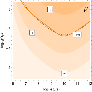
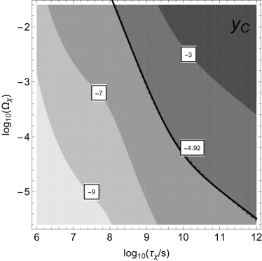
Figure 7: Contours of $\log_{10}(\delta\mu)$ (left panel) and $\log_{10}(\delta y_{C})$ (right panel) obtained from the analytic approximations in Eqs. (LABEL:eq:specfitsmu) and (73) in the presence of a single electromagnetically-decaying particle with extrapolated abundance $\Omega_{\chi}$ and lifetime $\tau_{\chi}$, plotted within the $(\Omega_{\chi},\tau_{\chi})$ plane. The gray dashed line in each panel demarcates the upper boundary of the region within the $(\Omega_{\chi},\tau_{\chi})$ plane which is consistent with the observed limits quoted in Eq. (56), while the solid curve represents the constraint contour obtained by fitting the corresponding analytic approximation in Eqs. (LABEL:eq:specfitsmu) and (73) to these numerical results.

We now determine the values of the parameters in Eqs. (LABEL:eq:specfitsmu) and (73) in a manner similar to that in which we determined the values of the parameters in Eqs. (LABEL:eq:BBNFitsTerm1)–(LABEL:eq:BBNFitsLi6). Specifically, we demand that our analytic approximations yield constraint contours consistent with those obtained from numerical analysis in the case in which the ensemble comprises a single decaying particle with lifetime $\tau_{\chi}$ and abundance $\Omega_{\chi}$. In particular, we survey $(\Omega_{\chi},\tau_{\chi})$ space and compute the generic spectral distortions numerically at each point using the Green’s-function formalism of Refs. ChlubaGreensFns1 ; ChlubaGreensFns2 . The generic spectra are then fit by a superposition of a $\mu$-type and a $y$-type distortion in order to determine a corresponding pair of values for $\delta\mu$ and $\delta y_{C}$. The undetermined parameters in Eqs. (LABEL:eq:specfitsmu) and (73) are then chosen such that our analytic expressions for $\delta\mu$ and $\delta y_{C}$ provide good fits to the corresponding constraint contours. Our best-fit values for all of these parameters are quoted in Table 3.

In Fig. 7, we display contours showing the results of our numerical calculations for $\delta\mu$ (left panel) and $\delta y_{C}$ (right panel) within the $(\Omega_{\chi},\tau_{\chi})$ plane. The gray dashed line in each panel demarcates the upper boundary of the region within the $(\Omega_{\chi},\tau_{\chi})$ plane which is consistent with the limits on these distortions quoted in Eq. (56). By contrast, the solid curve in each panel represents the corresponding constraint contour obtained through our analytic approximation in Eqs. (LABEL:eq:specfitsmu) and (73). As we see, the results obtained through our analytic approximation represent a good fit to our numerical results for both $\delta\mu$ and $\delta y_{C}$.

The constraint contours obtained from our analytic approximations for both $\mu$- and $y$-type distortions are also included in Fig. 6 in order to facilitate comparison with the constraint contours associated with the primordial abundances of light nuclei. We note that the constraint on $\delta\mu$ is more stringent than the constraint on $y_{C}$ for $\tau_{\chi}\lesssim t_{\mathrm{EC}}$, as expected, while the opposite is true for $\tau_{\chi}\gtrsim t_{\mathrm{EC}}$. We also see that both of these constraints are subdominant in comparison with the constraints on the primordial abundances of light nuclei, except at late times $\tau_{\chi}\gtrsim 10^{10}$ s.

V Modifications to the Ionization History of the Universe

As we have seen in Sect. IV, electromagnetic injection from late-decaying particles can give rise to certain distortions in the CMB-photon spectrum. However, such injections can affect the CMB in other ways as well. In particular, when such injection occurs during recombination, the resulting photons and electrons contribute to the heating and ionization of neutral hydrogen and helium as they cool, thereby expanding the surface of last scattering. This in turn leads to alterations in the pattern of CMB anisotropies, including a damping of correlations between temperature fluctuations as well as an enhancement of correlations between polarization fluctuations at low multipole moments ChenKamionkowski . These considerations therefore place additional constraints on decaying particle ensembles.

In a nutshell, these effects arise because the rates for many of the Class-I processes discussed in Sect. II are still sizable at times $t\sim t_{\mathrm{LS}}$. These processes therefore continue to rapidly redistribute the energies of photons injected during the recombination epoch to lower energies, thereby allowing for efficient photoionization of neutral hydrogen and helium at a rate that exceeds the rate of cosmic expansion. However, there is only a somewhat narrow time window around $t_{\mathrm{LS}}$ during which an injection of photons can have a significant impact on the surface of last scattering. At times $t\ll t_{\mathrm{LS}}$, any additional ionization of particles in the plasma is effectively washed out. By contrast, at times $t\gg t_{\mathrm{LS}}$, the relevant Class-I processes effectively shut off and photoionization is suppressed.

To a good approximation, then, we may regard any modification of the ionization history of the universe as being due to injection at $t\sim t_{\mathrm{LS}}$. Thus, the crucial quantity which is constrained is the overall injection rate of energy density in the form of photons or other electromagnetically-interacting particles at $t_{\mathrm{LS}}$. Since the universe is already matter-dominated by the recombination epoch, the injection rate associated with a single decaying particle species $\chi$ with lifetime $\tau_{\chi}$ and extrapolated abundance $\Omega_{\chi}$ at $t_{\mathrm{LS}}$ is given by

$$\left.\frac{d\rho_{\gamma}}{dt}\right|_{t=t_{\mathrm{LS}}}~{}=~{}\rho_{\mathrm{crit}}(t_{\mathrm{now}})\left(\frac{t_{\mathrm{now}}}{t_{\mathrm{LS}}}\right)^{2}\epsilon_{\chi}\frac{\Omega_{\chi}}{\tau_{\chi}}e^{-t_{\mathrm{LS}}/\tau_{\chi}}~{},$$ (74)

where $\epsilon_{\chi}$ once again denotes the fraction of the energy density released by $\chi$ decays which is transferred to photons. Thus, we model the constraint on such a decaying particle from its effects on the ionization history of the universe by an inequality of the form

$$\epsilon_{\chi}\frac{\Omega_{\chi}}{\tau_{\chi}}e^{-t_{\mathrm{IH}}/\tau_{\chi}}~{}\lesssim~{}\Gamma_{\mathrm{IH}}~{},~{}~{}$$ (75)

where $t_{\mathrm{IH}}$ and $\Gamma_{\mathrm{IH}}$ are taken to be free parameters.

We next determine the values of $\Gamma_{\mathrm{IH}}$ and $t_{\mathrm{IH}}$ by fitting these parameters to the constraint contours obtained in Refs. SlatyerInjectionHistory ; SlatyerWuIonizationUpdate from a numerical analysis of the injection and deposition dynamics. The constraint contours obtained from subsequent numerical studies by other authors PoulinIonization are quite similar. In particular, we find

$$\Gamma_{\mathrm{IH}} \approx 6.2\times 10^{-26}\mbox{~{}s}^{-1}$$

$$t_{\mathrm{IH}} \approx 1.4\times 10^{13}\mbox{~{}s}~{}.$$ (76)

Note that recent results from the final Planck data release PlanckFinal will affect the numerical values for $\Gamma_{\mathrm{IH}}$ and $t_{\mathrm{IH}}$ slightly but not dramatically.

In Fig. 8, we compare the results of our analytic approximation with the numerical results of Refs. SlatyerInjectionHistory ; SlatyerWuIonizationUpdate . We observe that our approximation for the constraint contour is in good agreement with these numerical results for $\tau_{\chi}\gtrsim 10^{15}$ s and deviates significantly from this contour only when $\tau_{\chi}\sim t_{\mathrm{LS}}$. However, as discussed in Ref. SlatyerInjectionHistory , the results to which we perform our fit yield an artificially conservative bound on $\Omega_{\chi}$ for lifetimes $\tau_{\chi}\sim t_{\mathrm{LS}}$, as the production of additional Lyman-$\alpha$ photons due to excitations from the ionizing particles was intentionally neglected. Other analyses of the ionization history ZhangChenKamionkowski which include this effect yield constraint contours which more closely resemble that obtained from our analytic approximation.

The constraint in Eq. (75) may be generalized to an ensemble of decaying particles in a straightforward manner. Indeed, since this constraint is ultimately a bound on the overall injection rate at $t\sim t_{\mathrm{LS}}$, the corresponding constraint on an ensemble of decaying particles $\chi_{i}$ takes the form

$$\sum_{i}\epsilon_{i}\frac{\Omega_{i}}{\tau_{i}}e^{-t_{\mathrm{IH}}/\tau_{i}}~{}\lesssim~{}\Gamma_{\mathrm{IH}}$$ (77)

with values of $\Gamma_{\mathrm{IH}}$ and $t_{\mathrm{IH}}$ once again given in Eq. (76).

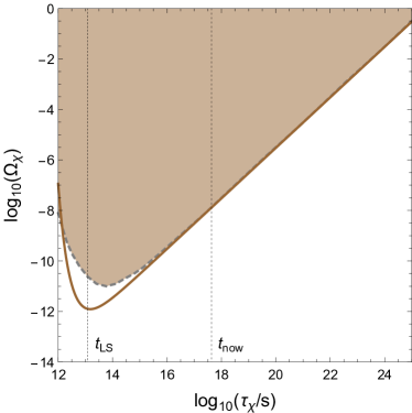
Figure 8: Constraints on a decaying particle with lifetime $\tau_{\chi}$ and extrapolated abundance $\Omega_{\chi}$ from modifications of the ionization history of the universe. These constraints correspond to the case in which $\epsilon_{\chi}=1$ and the entirety of the energy density released by $\chi$ decays is transferred to photons. The gray dashed contour represents the bound obtained in Refs. SlatyerInjectionHistory ; SlatyerWuIonizationUpdate from numerical analysis. The brown shaded region above the contour is excluded. The solid curve represents the constraint contour obtained by fitting the corresponding analytic approximation in Eq. (75) to these results. Dashed vertical lines indicating the time $t_{\mathrm{LS}}$ of last scattering and the present age of the universe $t_{\mathrm{now}}$ have also been included for reference. We see that our approximation for the constraint contour is in good agreement with these numerical results for $\tau_{\chi}\gtrsim 10^{15}$ s and deviates significantly from this contour only when $\tau_{\chi}\sim t_{\mathrm{LS}}$.

We emphasize that the constraint in Eq. (77) stems solely from the effect of electromagnetic injection from the decays of the ensemble constituents on the surface of last scattering. Since this effect arises primarily from injection at $t\sim t_{\mathrm{LS}}$, the constraints are most relevant for ensembles in which the constituents have lifetimes roughly around this timescale. However, electromagnetic injection can affect the ionization history of the universe in other ways as well. For example, energy deposited in the intergalactic medium as a result of particle decays at timescales well after $t_{\mathrm{LS}}$ serves both to elevate the gas temperature and to increase the ionization fraction of hydrogen. These effects can shift the onset of reionization to earlier times SlatyerWuIonizationUpdate ; SlatyerArbitraryInjections and impact the 21-cm absorption/emission signal arising from hyperfine transitions in neutral hydrogen ClarkDutta ; Liu21cm ; Mitridate21cm . These considerations are relevant primarily for particles with lifetimes $\tau_{i}\gg t_{\mathrm{now}}$ — particles which would in principle contribute to the present-day dark-matter abundance. Since our primary focus in this paper is on ensembles whose constituents have lifetimes $\tau_{i}\lesssim t_{\mathrm{now}}$, we do not investigate these additional considerations here. However, we note that they can play an important role in constraining ensembles of particles with longer lifetimes, such as those which arise within the context of the DDM framework.

VI Contributions to the Diffuse Photon Background

At times $t\gg t_{\mathrm{LS}}$, the universe becomes transparent to photons with a broad range of energies $\mathcal{O}(\mathrm{keV})\lesssim E_{\gamma}\lesssim\mathcal{O}(\mathrm{TeV})$ ChenKamionkowski . Photons within this energy range which are injected on timescales $t\gg t_{\mathrm{LS}}$ are not reprocessed by Class-I processes and do not interact with CMB photons at an appreciable rate. Thus, as discussed in Sect. IV, such photons therefore simply free-stream until the present epoch and contribute to the diffuse photon background. The total diffuse background of photons observed from the location of Earth includes both a galactic contribution from processes occurring within the Milky-Way halo (at redshifts $z\approx 0$) and an extra-galactic contribution from processes which occurred within the more distant past. The decays of unstable particles with lifetimes $\tau_{i}\ll t_{\mathrm{now}}$ contribute essentially exclusively to the extra-galactic component of this total background. By contrast, particles with lifetimes $\tau_{i}\gtrsim t_{\mathrm{now}}$ — particles which would contribute non-negligibly to the present-day abundance of dark matter — in principle contribute to both components. Since our primary focus in this paper is on particles with lifetimes in the regime $\tau_{i}\ll t_{\mathrm{now}}$, we focus on the extra-galactic component of the diffuse photon background. However, we also note that since the local dark-matter density within the Milky-Way halo is several orders of magnitude larger than the corresponding cosmological density, the galactic component of the diffuse photon background is typically the more important of the two for constraining particles with lifetimes $\tau_{i}\gtrsim t_{\mathrm{now}}$.

The overall diffuse extra-galactic contribution $d\Phi/dE_{\gamma}$ to the differential flux of photons per unit energy observed by a detector on Earth from the decays of an ensemble of unstable constituent particles $\chi_{i}$ is simply the direct sum of the individual contributions $d\Phi_{i}/dE_{\gamma}$ from these constituents. In order to evaluate these individual contributions, we begin by noting that the decays of a given species $\chi_{i}$, averaged over all possible decay channels, produce a characteristic injection spectrum of photons $d\mathcal{N}_{i}/dE_{\gamma}$. The spectrum of photons arriving at present time at a detector on Earth is the integrated total contribution from decays occurring at different redshifts. A photon injected at redshift $z$ with energy $E_{\gamma}^{\prime}$ is redshifted to energy $E_{\gamma}=(1+z)^{-1}E_{\gamma}^{\prime}$ when it arrives at the location of Earth. Thus, we find that the observed flux of photons observed at a detector on Earth from the decay of an individual decaying species $\chi_{i}$ may be written in the form

$$\frac{d\Phi_{i}}{dE_{\gamma}} = \frac{1}{4\pi}\int d\Omega\int_{0}^{\infty}dz\,\Bigg{\{}\frac{\rho_{i}(z)}{(1+z)^{3}}\frac{\Gamma_{i}}{m_{i}}\,\frac{d\ell}{dz}e^{-\kappa(z)}$$ (78)

$$~{}\times\int dE_{\gamma}^{\prime}\delta\left[E_{\gamma}^{\prime}-(1+z)E_{\gamma}\right]\frac{d\mathcal{N}_{i}}{dE_{\gamma}^{\prime}}\Bigg{\}}~{},~{}~{}~{}~{}~{}~{}$$

where $d\Omega$ is the differential solid angle of the detector, where $\rho_{i}(z)$ is the energy density of $\chi_{i}$ at redshift $z$, where $\kappa(z)$ is the optical depth of the universe to photons emitted at redshift $z$, and where $\ell(z)$ is the line-of-sight distance away from Earth, expressed as a function of $z$.

We focus here primarily on photons with energies in the range $\mathcal{O}(\mathrm{keV})\lesssim E_{\gamma}\lesssim\mathcal{O}(\mathrm{TeV})$, for which the universe is effectively transparent at all times $t\gtrsim t_{\mathrm{LS}}$ and opaque at times $t\lesssim t_{\mathrm{LS}}$. Moreover, for simplicity, we shall approximate the optical depth for such photons with a function of the form

$$\kappa(z)~{}\approx~{}\begin{cases}0&z<z_{\mathrm{LS}}\\ \infty&z>z_{\mathrm{LS}}~{},\end{cases}$$ (79)

where $z_{\mathrm{LS}}\equiv z(t_{\mathrm{LS}})\approx 1100$ is the redshift at the time of last scattering. In other words, we shall assume that the universe is completely transparent to all photons within this energy range after last scattering and completely opaque beforehand. Moreover, since $t_{\mathrm{LS}}\gg t_{\mathrm{MRE}}$, we approximate the line-of-sight distance $\ell(z)$ in a flat universe dominated by matter and dark energy as

$$\ell(z)~{}=~{}\frac{c}{H_{\mathrm{now}}}\int_{0}^{z}\frac{dz}{\mathcal{F}^{1/2}(z)}~{},$$ (80)

where $c$ is the speed of light, where $H_{\mathrm{now}}$ is the present-day value of the Hubble parameter, and where we have defined

$$\mathcal{F}(z)~{}\equiv~{}\Omega_{m}(1+z)^{3}+\Omega_{\Lambda}~{},$$ (81)

where $\Omega_{m}$ and $\Omega_{\Lambda}$ respectively denote the present-day abundances of massive matter and dark energy, the former including contributions from both dark and baryonic matter. The energy density $\rho_{i}(z)$ of a decaying particle can be expressed in terms of its extrapolated abundance $\Omega_{i}$ as

$$\rho_{i}(z)~{}=~{}\Omega_{i}\rho_{\mathrm{crit}}(t_{\mathrm{now}})(1+z)^{3}e^{-\Gamma_{i}t(z)}~{},$$ (82)

where the time $t(z)$ which corresponds to redshift $z$ is

$$t(z)~{}=~{}\frac{1}{H_{\mathrm{now}}}\int_{0}^{z}\frac{dz}{(1+z)\mathcal{F}^{1/2}(z)}~{}.$$ (83)

With these substitutions, Eq. (78) becomes

$$\frac{d\Phi_{i}}{dE_{\gamma}} = \frac{c\rho_{\mathrm{crit}}(t_{\mathrm{now}})\Omega_{i}\Gamma_{i}}{4\pi H_{\mathrm{now}}m_{i}}\!\int\!d\Omega\!\int_{0}^{z_{\mathrm{LS}}}\!\!dz\,\Bigg{[}\frac{1}{\mathcal{F}^{1/2}(z)}$$ (84)

$$~{}~{}~{}~{}~{}\times\,e^{-\Gamma_{i}t(z)}\left.\frac{d\mathcal{N}_{i}}{dE_{\gamma}^{\prime}}\right|_{E_{\gamma}^{\prime}=(1+z)E_{\gamma}}\Bigg{]}~{}.~{}~{}~{}$$

Finally, in assessing our prediction for $d\Phi/dE_{\gamma}$ for a decaying particle ensemble, we must account for the fact that at a realistic detector, the photon energies recorded by the instrument differ from the actual energies of the incoming photons due to the non-zero energy resolution of the detector. We account for this effect by convolving the spectrum of incoming photons with a smearing function $R_{\epsilon}(E_{\gamma}-E_{\gamma}^{\prime})$, which represents the probability for the detector to register a photon energy $E_{\gamma}$, given an actual incoming photon energy $E_{\gamma}^{\prime}$. For concreteness, we consider a Gaussian smearing function of the form

$$R_{\epsilon}(E_{\gamma}-E_{\gamma}^{\prime})~{}=~{}\frac{1}{\sqrt{2\pi}\epsilon E_{\gamma}^{\prime}}\exp\left[-\frac{(E_{\gamma}-E_{\gamma}^{\prime})^{2}}{2\epsilon^{2}E_{\gamma}^{\prime 2}}\right]~{},~{}~{}~{}$$ (85)

where $\epsilon$ is a dimensionless parameter which sets the overall, energy-dependent standard deviation $\sigma(E_{\gamma}^{\prime})=\epsilon E_{\gamma}^{\prime}$ of the distribution. Thus, we have our final result for the extra-galactic photon flux:

$$\frac{d\Phi}{dE_{\gamma}}~{}=~{}\sum_{i}\int dE_{\gamma}^{\prime}\frac{d\Phi_{i}}{dE_{\gamma}^{\prime}}R_{\epsilon}(E_{\gamma}-E_{\gamma}^{\prime})~{},$$ (86)

with the individual fluxes $d\Phi_{i}/dE_{\gamma}^{\prime}$ given by Eq. (84) and with $R_{\epsilon}(E_{\gamma}-E_{\gamma}^{\prime})$ given by Eq. (85).

Limits on additional contributions to the extra-galactic photon flux at energies $E_{\gamma}\gtrsim 800$ keV can be derived from measurements of the total gamma-ray flux by instruments such as COMPTEL, EGRET, and Fermi-LAT.  For photon energies in the range $800\mbox{~{}keV}\lesssim E_{\gamma}\lesssim 30\mbox{~{}MeV}$, COMPTEL data on the diffuse extra-galactic background spectrum COMPTELExGalPhotonBG are well modeled by a power-law expression of the form

$$\frac{d\Phi}{dE_{\gamma}d\Omega} \approx (49.9\times 10^{-3})\,\left(\frac{E_{\gamma}}{\mathrm{MeV}}\right)^{-2.40}$$ (87)

$$~{}~{}~{}~{}~{}~{}\mbox{~{}MeV}^{-1}\mathrm{cm}^{-1}\mathrm{s}^{-1}\mathrm{sr}^{-1}~{}.$$

Likewise, for energies in the range $30\mbox{~{}MeV}\lesssim E_{\gamma}\lesssim 1.41\mbox{~{}GeV}$, EGRET data EGRETExGalPhotonBG are well modeled by the power-law expression

$$\frac{d\Phi}{dE_{\gamma}d\Omega} \approx (7.35\times 10^{-3})\,\left(\frac{E_{\gamma}}{\mathrm{MeV}}\right)^{-2.35}$$ (88)

$$~{}~{}~{}~{}~{}~{}\mbox{~{}MeV}^{-1}\mathrm{cm}^{-1}\mathrm{s}^{-1}\mathrm{sr}^{-1}~{}.$$

At even higher energies, the spectrum of the extra-galactic diffuse photon background can be inferred from Fermi-LAT data. Within the energy range $100\mbox{~{}MeV}\lesssim E_{\gamma}\lesssim 820\mbox{~{}GeV}$, these data are well described by a power-law expression with an exponential suppression at high energies FermiExGalPhotonBG :

$$\frac{d\Phi}{dE_{\gamma}d\Omega} \approx (4.15\times 10^{-3})\,\left(\frac{E_{\gamma}}{\mathrm{MeV}}\right)^{\!-2.32}\!\!\!\!\exp\!\left(\frac{-E_{\gamma}}{279\mbox{~{}GeV}}\right)$$ (89)

$$~{}~{}~{}~{}~{}~{}~{}~{}~{}~{}~{}~{}~{}\mbox{~{}MeV}^{-1}\mathrm{cm}^{-1}\mathrm{s}^{-1}\mathrm{sr}^{-1}~{}.$$

Finally, we note that while we focus here primarily on photons with energies above $800$ keV, estimates of the extra-galactic photon background at lower energies have been computed from BAT BATExGalPhotonBG and INTEGRAL INTEGRALExGalPhotonBG data and from observations of Type-I supernovae SupernovaExGalPhotonBG .

The expression in Eq. (86) is completely general and applicable to any ensemble of particles which decays to photons with energies within the transparency window $\mathcal{O}(\mathrm{keV})\lesssim E_{\gamma}\lesssim\mathcal{O}(\mathrm{TeV})$. To illustrate how this expression can be evaluated in practice, we consider a concrete example involving a specific set of injection spectra $d\mathcal{N}_{i}/dE_{\gamma}$ for the ensemble constituents. In particular, we consider a scenario in which each constituent $\chi_{i}$ decays with a branching fraction of effectively unity to a pair of photons via the process $\chi_{i}\rightarrow\gamma+\gamma$. Under the assumption that the $\chi_{i}$ are “cold” (i.e., non-relativistic) by the time $t_{\mathrm{LS}}$, each of these photons has energy $E_{\gamma}\approx m_{i}/2$ in the comoving frame at the moment of injection. We thus have

$$\frac{d{\cal N}_{i}}{dE_{\gamma}}~{}\approx~{}2\delta\left(E_{\gamma}-\frac{m_{i}}{2}\right)~{}.$$ (90)

While higher-order processes will generically also give rise to a continuum spectrum which peaks around $E_{\gamma}\sim\mathcal{O}(10^{-3}m_{i})$, we focus here on the contribution from the photons with $E_{\gamma}\approx m_{i}/2$, since line-like features arising from monochromatic photon emission are far easier to detect than continuum features. Thus, for the injection spectrum in Eq. (90), the total contribution to the differential extra-galactic diffuse photon flux from the decays of the constituents within this ensemble is given by

$$\frac{d\Phi_{i}}{dE_{\gamma}} \approx \frac{c\rho_{\mathrm{crit}}(t_{\mathrm{now}})}{2\pi H_{\mathrm{now}}}\int\!d\Omega\int dE_{\gamma}^{\prime}\Bigg{\{}\frac{R_{\epsilon}(E_{\gamma}-E_{\gamma}^{\prime})}{E_{\gamma}^{\prime}}$$ (91)

$$\times\sum_{i}\frac{\Omega_{i}\Gamma_{i}}{m_{i}}\mathcal{F}^{-1/2}\!\left(\frac{m_{i}}{2E_{\gamma}^{\prime}}-1\right)$$

$$\times\,\exp\left[-\Gamma_{i}t\left(\frac{m_{i}}{2E_{\gamma}^{\prime}}-1\right)\right]\Bigg{\}}~{}.$$

VII Applications:  Two Examples

In Sects. III–VI, we examined the observational limits on electromagnetic injection from particle decays after the BBN epoch and formulated a set of constraints which can be broadly applied to any generic ensemble of unstable particles. In this section, we examine the implications of these constraints by applying them to a pair of toy ensembles which exhibit a variety of scaling behaviors for the constituent masses $m_{i}$, extrapolated abundances $\Omega_{i}$, and lifetimes $\tau_{i}$. For simplicity, we shall focus primarily on the “early-universe” regime in which $1\mbox{~{}s}\ll\tau_{i}\lesssim t_{\mathrm{LS}}$ for all of the $\chi_{i}$. Within this regime, the leading constraints on injection are those from modifications of the abundances of light nuclei and from distortions in the CMB.

We consider two different classes of mass spectra for our decaying ensemble constituents. The first consists of spectra in which the masses of these decaying particles are evenly distributed on a linear scale according to the scaling relation

$$m_{k}~{}=~{}m_{0}+k\,\Delta m~{},$$ (92)

where $k=0,1,...,N-1$ and where $m_{0}$ and $\Delta m$ are taken to be free parameters which describe the mass of the lightest ensemble constituent and the subsequent mass splittings respectively. Mass spectra of this approximate linear form are realized, for example, for the KK excitations of a particle propagating in a flat extra spacetime dimension whose total length is small compared with $1/m_{0}$. The second class of mass spectra we consider are spectra in which the particle masses are evenly distributed on a logarithmic scale according to the scaling relation

$$m_{k}~{}=~{}m_{0}\,\xi^{k}~{},$$ (93)

where $m_{0}$ once again denotes the mass of the lightest ensemble constituent, and where $\xi$ is a dimensionless free parameter. A mass spectrum of this sort is expected, for example, for axion-like particles in axiverse constructions Axiverse .

A variety of scaling relations for the decay widths $\Gamma_{i}$ of the $\chi_{i}$ across the ensemble can likewise be realized in different scenarios. For simplicity, in this paper we focus on the case in which each $\chi_{i}$ decays with a branching fraction of effectively unity to a pair of photons via the process $\chi_{i}\rightarrow\gamma+\gamma$. Moreover, we shall assume that the scaling relation for $\Gamma_{i}$ takes the form

$$\Gamma_{i}~{}=~{}C_{i}\frac{m_{i}^{3}}{\Lambda^{2}}~{},$$ (94)

where $\Lambda$ is a parameter with dimensions of mass and where $C_{i}$ is a dimensionless coefficient — a coefficient which in principle can also have a non-trivial dependence on $m_{i}$. Such a scaling relation arises naturally, for example, in situations in which each of the $\chi_{i}$ decays via a non-renormalizable Lagrangian operator of dimension $d=5$ in an effective theory for which $\Lambda$ is the cutoff scale. For purposes of illustration, we focus on the case in which the coefficient $C_{i}=C_{\chi}$ is identical for all $C_{i}$. In this case, the $\Gamma_{i}$ are specified by a single free parameter: the ratio $M_{\ast}\equiv\Lambda/\sqrt{C_{\chi}}$. We emphasize that it is possible — and indeed in most situations even expected — that $C_{\chi}\ll 1$. Thus, unlike $\Lambda$ itself, the parameter $M_{\ast}$ may exceed the reduced Planck mass $M_{P}$ without necessarily rendering the theory inconsistent. However, we remark that for values of $M_{\ast}$ in this regime, the Weak Gravity Conjecture WeakGravityConjecture imposes restrictions on the manner in which the decay operator in Eq. (94) can arise.

Finally, we consider a range of different possible scaling relations for the extrapolated abundances $\Omega_{i}$ across the ensemble. In particular, we consider a family of scaling relations for the $\Omega_{i}$ of the form

$$\Omega_{i}~{}=~{}\Omega_{0}\left(\frac{m_{i}}{m_{0}}\right)^{\gamma}~{},$$ (95)

in which the abundance $\Omega_{0}$ of the lightest ensemble constituent and the scaling exponent $\gamma$ are both taken to be free parameters. In principle, $\gamma$ can be either positive or negative. However, since $\tau_{i}\propto m_{i}^{-3}$ and since the leading constraints on injection at timescales $t_{\mathrm{inj}}\lesssim t_{\mathrm{LS}}$ are typically less stringent for earlier $t_{\mathrm{inj}}$, the most interesting regime turns out to be that in which $\gamma\geq 0$ and the initial energy density associated with each $\chi_{i}$ is either uniform across the ensemble or decreases with increasing $\tau_{i}$.

In summary, then, each of our toy ensembles is characterized by a set of six parameters: $\{N,m_{0},\Delta m,M_{\ast},\Omega_{0},\gamma\}$ for the mass spectrum in Eq. (92) and $\{N,m_{0},\xi,M_{\ast},\Omega_{0},\gamma\}$ for the mass spectrum in Eq. (93). Note that for any particular choice of these parameters, the lifetimes of the individual ensemble constituents span a range $\tau_{N-1}\leq\tau_{i}\leq\tau_{0}$.

VII.1 Results for Uniform Mass Splittings

We begin by examining the results for a toy ensemble with a mass spectrum given by Eq. (92). For such a mass spectrum, the density $n_{m}$ of states per unit mass is uniform across the ensemble; however, it is also useful to consider the density $n_{\tau}$ of states per unit lifetime, which is more directly related to the injection history. In the continuum limit in which the difference between the lifetimes of sequential states $\chi_{i}$ and $\chi_{i+1}$ in the ensemble is small and the lifetime $\tau$ may be approximated as a continuous variable, we find that

$$n_{\tau}~{}=~{}\frac{M_{\ast}^{2/3}}{3\,\Delta m\,\tau^{4/3}}~{}.$$ (96)

The density of states per unit lifetime is therefore greatest within the most unstable regions of the ensemble. Moreover, we also note that the density of states per unit $\ln(\tau)$ also decreases with $\ln(\tau)$. These considerations turn out to have important implications for the bounds on such ensembles, as shall become apparent below.

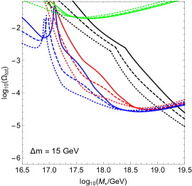
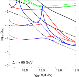
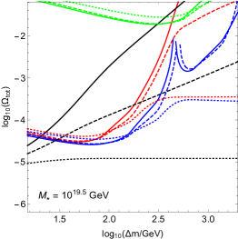
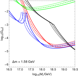
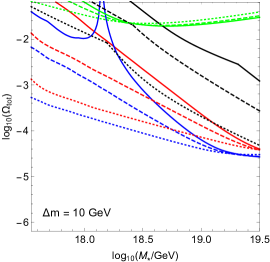
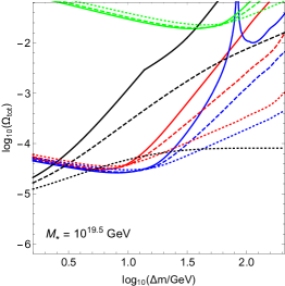
Figure 9: Compilation of constraints on electromagnetic injection for “low-density” ensembles with mass spectra of the form given in Eq. (92), in which the mass splitting $\Delta m$ between successive $\chi_{i}$ is constant. The contours shown correspond to the choice of $N=3$ with $m_{0}=10$ GeV.  The curves shown in each panel indicate the upper bound on the total abundance $\Omega_{\mathrm{tot}}$ of the ensemble from constraints on the primordial abundances of $\ce{D}$ (blue curve), $\ce{{}^{7}Li}$ (green curve), and $\ce{{}^{6}Li}$ (red curve) and from limits on distortions of the CMB-photon spectrum (black curve). The dotted, dashed, and solid curves correspond respectively to the choices $\gamma=\{0,1,2\}$ for the scaling exponent in Eq. (95). In the left and center panels, we plot this upper bound as a function of the coupling-suppression scale $M_{\ast}$ with fixed $\Delta m=15$ GeV and with fixed $\Delta m=95$ GeV, respectively. In the right panel, we plot the bound as a function of $\Delta m$ with fixed $M_{\ast}=10^{19.5}$ GeV. Comparing the results shown in the center panel with those of Fig. 6, we see that the bounds on a decaying ensemble differ not only quantitatively but even qualitatively from the bounds on its individual constituents.

Figure 10: Same as in Fig. 10, but for “high-density” ensembles with $N=20$. In the left and center panels, we plot the upper bound on $\Omega_{\mathrm{tot}}$ as a function of the coupling-suppression scale $M_{\ast}$ with fixed $\Delta m=1.58$ and with fixed $\Delta m=10$ GeV, respectively. In the right panel, we plot the bound as a function of $\Delta m$ with fixed $M_{\ast}=10^{19.5}$ GeV.

In Fig. 10, we show the constraints on an ensemble comprising $N=3$ unstable particles in which the lightest ensemble constituent has a mass $m_{0}=10$ GeV.  We consider this ensemble to be “low-density” in that it has a density of states per unit $\tau$ which is small throughout the range of parameters shown. (This will later be contrasted with analogous results in Fig. 10 for a “high-density” ensemble.) The contours shown in the left and center panels of Fig. 10 represent upper bounds on the total extrapolated abundance $\Omega_{\mathrm{tot}}$ as functions of $M_{\ast}$ for fixed $\Delta m$. The contours shown in the left panel correspond to the choice of $\Delta m=15$ GeV; those in the center panel correspond to the choice of $\Delta m=95$ GeV.  In the right panel, we show the corresponding contours as functions of $\Delta m$ for fixed $M_{\ast}=10^{19.5}$ GeV.  The blue, green, and red curves shown in each panel represent the bounds on $\Omega_{\mathrm{tot}}$ from constraints on the primordial abundances of $\ce{D}$, $\ce{{}^{7}Li}$, and $\ce{{}^{6}Li}$, respectively. We use a uniform color for the $\ce{D}$ contour — a contour which reflects the sum of contributions to $\delta Y_{\ce{D}}$ from both production and destruction processes. The dotted, dashed, and solid curves of each color correspond respectively to the choices $\gamma=\{0,1,2\}$ for the scaling exponent in Eq. (95). The corresponding black curves shown in each panel represent the bounds arising from limits on distortions of the CMB-photon spectrum obtained by taking whichever bound (either that from $\delta\mu$ or that from $\delta y_{C}$) is more stringent at every point.

In interpreting the results shown in Fig. 10, we note that each choice of parameters specifies a particular range of lifetimes $\tau_{N-1}\leq\tau_{i}\leq\tau_{0}$ for the ensemble constituents. This range of lifetimes varies across the range of $M_{\ast}$ shown in the left panel, from $1.03\times 10^{4}\mathrm{~{}s}\leq\tau_{i}\leq 6.58\times 10^{5}\mbox{~{}s}$ for $M_{\ast}=10^{16.5}$ GeV to $1.03\times 10^{10}\mathrm{~{}s}\leq\tau_{i}\leq 6.58\times 10^{11}\mathrm{~{}s}$ for $M_{\ast}=10^{19.5}$ GeV.  Across this entire range of $M_{\ast}$ values, the range of $\tau_{i}$ values for the ensemble is reasonably narrow, spanning only roughly a single order of magnitude. As a result, the bounds on $\Omega_{\mathrm{tot}}$ for a decaying ensemble shown in the left panel of Fig. 10 as functions of $M_{\ast}$ closely resemble the bounds on $\Omega_{\chi}$ for a single decaying particle species shown in Fig. 6 as a function of $\tau_{\chi}$. Moreover, since the $\tau_{i}$ for all particles in the ensemble are roughly comparable, the results are not particularly sensitive to $\gamma$, which determines how $\Omega_{\mathrm{tot}}$ is distributed across the ensemble. The most stringent constraint on $\Omega_{\mathrm{tot}}$ is the bound associated with the primordial $\ce{D}$ abundance over almost the entire range of $M_{\ast}$ shown. The only exception occurs in the regime where $M_{\ast}$ is large and the lifetimes of all of the ensemble constituents are extremely long, in which case the constraint associated with CMB distortions supersedes the $\ce{D}$ constraint. We note that for values of $\Omega_{\mathrm{tot}}$ which lie above the $\ce{D}$ contour, $\ce{D}$ may be either overabundant or underabundant. We also note that a “funnel” similar to that appearing in Fig. 6 is visible in the $\ce{D}$ constraint contours for all values of $\gamma$ shown in the figure, and that this funnel occurs where $M_{\ast}$ is such that the lifetimes of the ensemble constituents are approximately $\tau_{i}\approx 10^{6.5}$ s.

By contrast, the results shown in the center panel of Fig. 10 correspond to the regime in which the range of lifetimes spanned by the ensemble is quite broad, extending over several orders of magnitude in $\tau_{i}$. In particular, the range of lifetimes varies across the range of $M_{\ast}$ shown in this panel from $1.03\times 10^{4}\mathrm{~{}s}\leq\tau_{i}\leq 8.22\times 10^{7}\mbox{~{}s}$ for $M_{\ast}=10^{17.5}$ GeV to $8.22\times 10^{7}\mathrm{~{}s}\leq\tau_{i}\leq 6.58\times 10^{11}\mathrm{~{}s}$ for $M_{\ast}=10^{19.5}$ GeV.  We note that the range of $M_{\ast}$ shown in this panel has been truncated relative to the left panel in order to ensure that the characteristic decay timescales for all ensemble constituents occur well after the BBN epoch. For an ensemble with such a broad range of lifetimes, the effect of distributing $\Omega_{\mathrm{tot}}$ over multiple particle species is readily apparent. Indeed, the shapes of the constraint contours in the center panel of Fig. 10 bear little resemblance to the shapes of the contours in Fig. 6. Thus, comparing the results shown in the center panel of Fig. 10 with those in Fig. 6, we see that the bounds on a decaying ensemble indeed differ not only quantitatively but even qualitatively from the bounds on its individual constituents.

For example, two separate funnels arise in the $\ce{D}$ constraint contour for $\gamma=2$. Each of these funnels represents not merely a cancellation between the production and destruction contributions to $Y_{\ce{D}}$ from a single particle, but rather a cancellation among the individual contributions from all constituent particle species in the ensemble. The funnel on the left arises due to a cancellation between the net negative contributions to $Y_{\ce{D}}$ from $\chi_{1}$ and $\chi_{2}$ and the net positive contribution from $\chi_{0}$. By contrast, the funnel on the right arises due to a cancellation between a net negative contribution to $Y_{\ce{D}}$ from $\chi_{2}$ and positive contributions from $\chi_{0}$ and $\chi_{1}$, with the latter contribution suppressed because $\tau_{1}\approx 10^{6.5}$ s. The positions of these funnels, then, reflect the collective nature of the ensemble — and they have important consequences. Indeed, within certain regions of parameter space within which the $\ce{D}$ constraints are weakened by cancellations among $\delta Y_{\ce{D}}$ contributions from different ensemble constituents, the constraint associated with the $\ce{{}^{6}Li}$ abundance actually represents the leading bound on $\Omega_{\mathrm{tot}}$ for the ensemble.

Finally, in the right panel of Fig. 10, we show how the bounds on $\Omega_{\mathrm{tot}}$ vary as a function of $\Delta m$ for fixed $M_{\ast}=10^{19.5}$ GeV.  We choose this benchmark for $M_{\ast}$ because the CMB-distortion constraints and the leading constraints from light nuclei are comparable for this choice of $M_{\ast}$. In interpreting the results displayed in this panel, it is important to note that $\tau_{0}$ is independent of $\Delta m$. By contrast, the $\tau_{i}$ for all other $\chi_{i}$ decrease with increasing $\Delta m$. Since, broadly speaking, the impact that a decaying particle has on both CMB distortions and on the primordial abundances of light nuclei tends to decrease as $\tau_{i}$ decreases, the bounds on decaying ensembles generally grow weaker as $\Delta m$ increases. This weakening of the constraints generally grows more pronounced as $\gamma$ increases and as a larger fraction of the abundance is carried by the heavier ensemble constituents. For $\gamma=0$, on the other hand, the fraction of $\Omega_{\mathrm{tot}}$ carried by the lightest ensemble constituent $\chi_{0}$ is independent of $\Delta m$. As a result, many of the constraint contours shown in the right panel of Fig. 10 become essentially flat for sufficiently large $\Delta m$ as the lifetimes of the remaining $\chi_{i}$ become so short that the impact of their decays on the corresponding cosmological observables is negligible in comparison with those of $\chi_{0}$.

Thus far, we have focused on the regime in which the spacing between the lifetimes $\tau_{i}$ of the ensemble constituents is large — in other words, the regime in which the density of states per unit $\tau$ is small across the ensemble. However, it is also interesting to consider the opposite regime, in which the density of states per unit $\tau$ is sufficiently large over the entire range $\tau_{N-1}\leq\tau\leq\tau_{0}$ that the ensemble effectively acts as a continuous source of electromagnetic injection over this interval. This range of lifetimes is completely determined in our toy model by $M_{\ast}$, $m_{0}$, and the quantity $m_{N-1}=(N-1)\Delta m+m_{0}$. Thus, we may make a direct comparison between the bounds on such “high-density ensembles” and the bounds on “low-density” ensembles with the same $\tau_{i}$ range by varying $N$ and $\Delta m$ oppositely while holding $M_{\ast}$, $m_{0}$, and $m_{N-1}$ fixed. Towards this end, in Fig. 10, we show the upper bounds on $\Omega_{\mathrm{tot}}$ for an ensemble with a higher density of states per unit lifetime. The constraint contours in the left and center panels of the figure represent the same choices of $m_{0}$ and $m_{N-1}$ as in the corresponding panels of Fig. 10, but for $N=20$ rather than $N=3$. For these parameter choices, the ensemble is effectively in the “high-density” regime over the entire range of $M_{\ast}$ shown in each panel. In the right panel of Fig. 10, we once again show constraint contours as functions of $\Delta m$ for fixed $M_{\ast}$.

As one might expect, the primary effect of distributing the abundance of the ensemble more evenly across the same range of lifetimes is that features in the constraint contours associated with particular $\chi_{i}$ are in large part smoothed out. While the $\ce{D}$ funnels in the left panel are still present, this reflects the fact that the range of $\tau_{i}$ for the ensemble is sufficiently narrow that distributing the abundance more democratically across this range has little impact on the constraint contours. A single $\ce{D}$ funnel also appears in the constraint contour for $\gamma=2$ in the center panel of Fig. 10. The presence of this feature reflects the fact that for $\gamma=2$, the vast majority of $\Omega_{\mathrm{tot}}$ is carried by the most massive — and therefore most unstable — ensemble constituents. Moreover, the density of states per unit lifetime is also much higher for these shorter-lived states than it is for the rest of the ensemble. The funnel can be understood as corresponding to the value of $M_{\ast}$ for which the lifetimes of these states, which are smaller than but roughly similar to $\tau_{N-1}$, satisfy $\tau_{i}\sim\tau_{N-1}\approx 10^{6.5}$ s. Once again, however, we note that the location of the funnel is shifted slightly away from this value of $M_{\ast}$ due to the collective contribution to $Y_{D}$ from the longer-lived constituents in the ensemble. A similar feature is also apparent in the constraint contour for $\gamma=2$ in the right panel of Fig. 10.

We can gain further insight into the results displayed in Fig. 10 by examining the continuum limit in which $\Delta m\rightarrow 0$. In this limit, the sums appearing in Eqs. (LABEL:eq:BBNFitsTerm1)–(LABEL:eq:BBNFitsLi6) and in Eqs. (LABEL:eq:specfitsmu) and (73) can be recast as integrals over the continuous lifetime variable $\tau$ — integrals which may be evaluated in a straightforward manner, yielding analytic expressions for $\delta Y_{a}$, $\delta\mu$, and $\delta y_{C}$. For example, in the case in which the $\tau_{i}$ span the entire range from $t_{Aa}$ to $t_{fa}$ for each relevant nucleus, we find that for any $\gamma\geq 0$ the term $\delta Y_{a}^{(1)}$ in Eq. (51) takes the form

$$\delta Y_{a}^{(1)} = A_{a}\Xi(t_{Ca})\Gamma\left(\frac{\gamma}{3}-\frac{2}{3},x^{-1}\right)\Bigg{|}_{x^{\mathrm{min}}_{Aa}}^{x^{\mathrm{max}}_{Aa}}$$

$$+ \!\!\!\!\!B_{a}\Xi(t_{Xa})\Bigg{[}\frac{6\beta x^{-\frac{5+2\gamma}{6}}}{5+2\gamma}-\frac{3x^{-\frac{1+\gamma}{3}}}{1+\gamma}\Bigg{]}\Bigg{|}_{x^{\mathrm{min}}_{Ba}}^{x^{\mathrm{max}}_{Ba}}$$

$$+ \!\!\!\!\!B_{a}\Xi(t_{Xa})\Bigg{[}\frac{6(1+\beta)x^{-\frac{5+2\gamma}{6}}}{5+2\gamma}-\frac{24x^{-\frac{7+4\gamma}{12}}}{7+4\gamma}\Bigg{]}\Bigg{|}_{x^{\mathrm{min}}_{Ca}}^{x^{\mathrm{max}}_{Ca}}~{},$$

where $\Gamma(n,z)$ is the incomplete gamma function, where we have defined

$$\Xi(t)~{}\equiv~{}\frac{(\gamma+1)\Omega_{\mathrm{tot}}M_{\ast}^{2(1+\gamma)/3}}{3\big{(}m_{N-1}^{\gamma+1}-m_{0}^{\gamma+1}\big{)}t^{(1+\gamma)/3}}~{},$$ (98)

where $A_{a}$ and $B_{a}$ are defined in Table 2 and where the limits of integration are

$$\begin{array}[]{ll}x^{\mathrm{min}}_{Aa}~{}=~{}t_{Aa}/t_{Ca}{}{}{}{}&~{}~{}~{}~{}x^{\mathrm{max}}_{Aa}~{}=~{}t_{Ba}/t_{Ca}\\ x^{\mathrm{min}}_{Ba}~{}=~{}t_{Ba}/t_{Xa}{}{}{}{}&~{}~{}~{}~{}x^{\mathrm{max}}_{Ba}~{}=~{}1\\ x^{\mathrm{min}}_{Ca}~{}=~{}1{}{}{}{}&~{}~{}~{}~{}x^{\mathrm{max}}_{Ca}~{}=~{}t_{fa}/t_{Xa}~{}.\end{array}$$ (99)

In cases in which $\tau_{i}$ does not span the entire range from $t_{Aa}$ to $t_{fa}$, the values of the quantities in Eq. (99) should be replaced by values which restrict the overall range of lifetimes to $\max[\tau_{N-1},t_{Aa}]\leq\tau_{i}\leq\min[\tau_{0},t_{fa}]$.

For $\ce{D}$ and $\ce{{}^{6}Li}$, the term $\delta Y_{a}^{(2)}$ in Eq. (51) is non-vanishing and must be evaluated separately. For $\ce{D}$, the term $\delta Y_{a}^{(2)}$ in Eq. (51) has exactly the same form as Eq. (LABEL:eq:ContLimitBBNLinear), but with $A^{\ast}_{a}$ in place of $A_{a}$, $B^{\ast}_{a}$ in place of $B_{a}$, etc.  For $\ce{{}^{6}Li}$, we find for all $\gamma\geq 0$ that the $\delta Y_{a}^{(2)}$ term takes the form

$$\delta Y_{a}^{(2)} = A^{*}_{a}\Xi(t^{*}_{Ca})\Gamma\left(\frac{\gamma}{3}-\frac{2}{3},x^{-1}\right)\Bigg{|}_{x^{\ast\mathrm{min}}_{Aa}}^{x^{\ast\mathrm{max}}_{Aa}}$$

$$+ \!\!\!\!\!\!\!B^{*}_{a}\Xi(t^{*}_{Xa})\Bigg{[}\frac{72\beta^{5}\theta x^{-\frac{17+2\gamma}{6}}}{17+2\gamma}-\frac{45\beta^{4}(1+\theta)x^{-\frac{7+\gamma}{3}}}{7+\gamma}+\frac{120\beta^{3}x^{-\frac{11+2\gamma}{6}}}{11+2\gamma}-\frac{3(5-3\theta)x^{-\frac{1+\gamma}{3}}}{1+\gamma}\Bigg{]}\Bigg{|}_{x^{\ast\mathrm{min}}_{Ba}}^{x^{\ast\mathrm{max}}_{Ba}}$$

$$+ \!\!\!\!\!\!\!B^{*}_{a}\Xi(t^{*}_{Xa})\Bigg{[}\frac{8\theta(1+9\beta^{5})x^{-\frac{17+2\gamma}{6}}}{17+2\gamma}-\frac{45(1+\theta)(1+7\beta^{4})x^{-\frac{7+\gamma}{3}}}{7(7+\gamma)}+\frac{24(1+5\beta^{3})x^{-\frac{11+2\gamma}{6}}}{11+2\gamma}-\frac{64(9-5\theta)x^{-\frac{7+4\gamma}{12}}}{7(7+4\gamma)}\Bigg{]}\Bigg{|}_{x^{\ast\mathrm{min}}_{Ca}}^{x^{\ast\mathrm{max}}_{Ca}}~{},$$

where the limits of integration are given by expressions analogous to those appearing in Eq. (99).

Expressions for the CMB-distortion parameters $\delta\mu$ and $\delta y_{C}$ may be obtained in a similar fashion. In particular, for the case in which the $\tau_{i}$ span the entire range from $t_{e}$ to $t_{\mathrm{LS}}$, we find that $\delta\mu$ takes the form

$$\delta\mu = \frac{4A_{\mu}}{5}\Xi(t_{0\mu})\Gamma\left(\frac{4\gamma-2}{15},x^{-5/4}\right)\Bigg{|}_{x^{\mathrm{min}}_{0\mu}}^{x^{\mathrm{max}}_{0\mu}}$$ (101)

$$~{}+B_{\mu}\Xi(t_{1\mu})\Bigg{[}\frac{6}{1-2\gamma}x^{\frac{1-2\gamma}{6}}-\frac{1}{\alpha_{\mu}}\Gamma\left(\frac{2\gamma-1}{6\alpha_{\mu}},x^{-\alpha_{\mu}}\right)\Bigg{]}\Bigg{|}_{x^{\mathrm{min}}_{1\mu}}^{x^{\mathrm{max}}_{1\mu}}$$

$$~{}+B_{\mu}\Xi(t_{2\mu})\Bigg{[}\frac{3}{1-\gamma}x^{\frac{1-\gamma}{3}}-\frac{3}{4\alpha_{\mu}}\Gamma\left(\frac{\gamma-1}{4\alpha_{\mu}},x^{-\frac{4\alpha_{\mu}}{3}}\right)\Bigg{]}\Bigg{|}_{x^{\mathrm{min}}_{2\mu}}^{x^{\mathrm{max}}_{2\mu}}$$

for all $\gamma\geq 0$, except for the special case in which $\gamma=1$. For this special case, the replacement

$$-\frac{3}{1-\gamma}x^{\frac{1-\gamma}{3}}~{}\longrightarrow~{}\ln x$$ (102)

should be made in the fourth line of Eq. (101). Likewise, we find that $\delta y_{C}$ takes the form

$$\delta y_{C} = \frac{4A_{y}}{5}\Xi(t_{0y})\left.\Gamma\left(\frac{4\gamma-2}{15},x^{-5/4}\right)\right|_{x^{\mathrm{min}}_{0y}}^{x^{\mathrm{max}}_{0y}}$$ (103)

$$~{}+B_{y}\Xi(t_{1y})\frac{6x^{\alpha+\frac{1-2\gamma}{6}}}{6\alpha_{\mu}-2\gamma+1}\left.{}_{2}F_{1}\left(1,1+\frac{1-2\gamma}{6\alpha_{y}};2+\frac{1-2\gamma}{6\alpha_{y}};-x^{\alpha_{y}}\right)\right|_{x^{\mathrm{min}}_{1y}}^{x^{\mathrm{max}}_{1y}}$$

$$~{}+B_{y}\Xi(t_{2y})\frac{3x^{\frac{1-\gamma}{3}}}{1-\gamma}\left.{}_{2}F_{1}\left(1,\frac{\gamma-1}{4\alpha_{y}};1+\frac{\gamma-1}{4\alpha_{y}};-x^{-\frac{4\alpha_{y}}{3}}\right)\right|_{x^{\mathrm{min}}_{2y}}^{x^{\mathrm{max}}_{2y}}~{},$$

where ${}_{2}F_{1}(a,b;c;z)$ denotes the ordinary hypergeometric function, where $A_{a}$, $B_{a}$, and $\alpha_{a}$ are defined in Table 3, and where the limits of integration are

$$\begin{array}[]{ll}x^{\mathrm{min}}_{0a}~{}=~{}t_{e}/t_{0a}{}{}{}{}&~{}~{}~{}~{}x^{\mathrm{max}}_{0a}~{}=~{}t_{Ba}/t_{0a}\\ x^{\mathrm{min}}_{1a}~{}=~{}t_{Ba}/t_{1a}{}{}{}{}&~{}~{}~{}~{}x^{\mathrm{max}}_{1a}~{}=~{}t_{\mathrm{MRE}}/t_{1a}\\ x^{\mathrm{min}}_{2a}~{}=~{}t_{\mathrm{MRE}}/t_{2a}{}{}{}{}&~{}~{}~{}~{}x^{\mathrm{max}}_{2a}~{}=~{}t_{\mathrm{LS}}/t_{2a}~{}.\end{array}$$ (104)

Once again, in cases in which $\tau_{i}$ does not span the entire range from $t_{e}$ to $t_{\mathrm{LS}}$, the values of the quantities in Eq. (104) should be replaced by values which restrict the overall range of lifetimes to $\max[\tau_{N-1},t_{e}]\leq\tau_{i}\leq\min[\tau_{0},t_{\mathrm{LS}}]$.

VII.2 Results for Exponentially Rising Mass Splittings

We now consider the results for a toy ensemble with a mass spectrum given by Eq. (93). The density of states per unit mass is inversely proportional to $m$ in this case, and the corresponding density of states per unit lifetime is

$$n_{\tau}~{}=~{}\frac{1}{3\ln(\xi)\tau}~{},$$ (105)

which likewise decreases with $\tau$. However, we note that the density of states per unit $\ln(\tau)$ in this case remains constant across the ensemble.

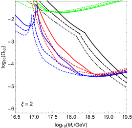
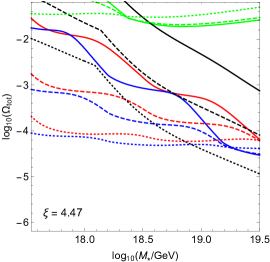
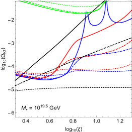
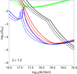
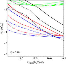
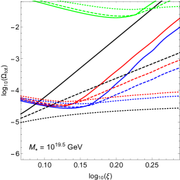
Figure 11: Same as in Fig. 10, but for “low-density” ensembles with mass spectra of the form given in Eq. (93), in which the masses of the $\chi_{i}$ are evenly distributed on a logarithmic scale. In the left and center panels, we plot the upper bound on $\Omega_{\mathrm{tot}}$ as a function of the coupling-suppression scale $M_{\ast}$ with fixed $\xi=2$ and with fixed $\xi=4.47$, respectively. In the right panel, we plot the bound as a function of $\xi$ with fixed $M_{\ast}=10^{19.5}$ GeV.

Figure 12: Same as in Fig. 12, but for “high-density” ensembles with $N=10$. In the left and center panels, we plot the upper bound on $\Omega_{\mathrm{tot}}$ as a function of the coupling-suppression scale $M_{\ast}$ with fixed $\xi=1.2$ and with fixed $\xi=1.39$, respectively. In the right panel, we plot the bound as a function of $\xi$ with fixed $M_{\ast}=10^{19.5}$ GeV.

In Fig. 12 we show the bounds on $\Omega_{\mathrm{tot}}$ for a “low-density” ensemble with a mass spectrum given by Eq. (93) and the same benchmark parameter choices $N=3$ and $m_{0}=10$ GeV as in Fig. 10. In the left and center panels, the value of $\xi$ has been chosen such that the range of $\tau_{i}$ for the ensemble constituents is the same as in Fig. 10 at both ends of the range of $M_{\ast}$ shown. For the mass spectrum considered here, this range of $\tau_{i}$ depends on $m_{0}$, on $M_{\ast}$, and on the quantity $\xi^{N-1}$. In the right panel of Fig. 12, we show how the bounds on $\Omega_{\mathrm{tot}}$ vary as a function of $\xi$ for fixed $M_{\ast}=10^{19.5}$ GeV.  The contours shown in Fig. 12 exhibit the same overall scaling behaviors as those in Fig. 10. However, there are salient differences which reflect the fact that the density of states per unit $\ln(\tau)$ is uniform in this case across the ensemble.

In Fig. 12, we show the corresponding results for an ensemble with $m_{0}=10$ GeV and a mass spectrum again given by Eq. (93), but with a sufficiently high $n_{\tau}$ throughout the range of $M_{\ast}$ or $\xi$ shown in each panel that the ensemble is effectively always within the “high-density” regime. We find that taking $N=10$ is sufficient to achieve this. The left and center panels of Fig. 12 correspond to the same ranges of $M_{\ast}$ and the same value of $\xi^{N-1}$ as the left and center panels of Fig. 12. The right panel once again shows how the bounds on $\Omega_{\mathrm{tot}}$ vary as a function of $\xi$ for fixed $M_{\ast}=10^{19.5}$ GeV.  Once again, we see that the principal consequence of increasing $n_{\tau}$ is that constraint contours become increasingly smooth and featureless.

Once again, as we did for the case of an ensemble with a uniform mass splitting, we may derive the corresponding expressions for $\delta Y_{a}$, $\delta\mu$, and $\delta y_{C}$ in the case of an exponentially rising mass splitting in the continuum limit by direct integration of the expressions in Eqs. (LABEL:eq:BBNFitsTerm1)–(LABEL:eq:BBNFitsLi6) and in Eqs. (LABEL:eq:specfitsmu) and (73). For the mass spectrum in Eq. (93), this limit corresponds to taking $\xi\rightarrow 1$. For the case in which the $\tau_{i}$ span the entire range from $t_{Aa}$ to $t_{fa}$ for each relevant nucleus, we find that for $\gamma>0$, the term $\delta Y_{a}^{(1)}$ in Eq. (51) takes the form

$$\delta Y_{a}^{(1)} = A_{a}\widetilde{\Xi}(t_{Ca})\Gamma\left(\frac{\gamma}{3}-1,x^{-1}\right)\Bigg{|}_{x^{\mathrm{min}}_{Aa}}^{x^{\mathrm{max}}_{Aa}}$$

$$+ \!\!\!\!\!\!\!B_{a}\widetilde{\Xi}(t_{Xa})\Bigg{[}\frac{6\beta x^{-\frac{3+2\gamma}{6}}}{3+2\gamma}-\frac{3x^{-\frac{\gamma}{3}}}{\gamma}\Bigg{]}\Bigg{|}_{x^{\mathrm{min}}_{Ba}}^{x^{\mathrm{max}}_{Ba}}$$

$$+ \!\!\!\!\!\!\!B_{a}\widetilde{\Xi}(t_{Xa})\Bigg{[}\frac{6(1+\beta)x^{-\frac{3+2\gamma}{6}}}{3+2\gamma}-\frac{24x^{-\frac{3+4\gamma}{12}}}{3+4\gamma}\Bigg{]}\Bigg{|}_{x^{\mathrm{min}}_{Ca}}^{x^{\mathrm{max}}_{Ca}}~{},$$

where the limits of integration are defined as in Eq. (99) and where we have defined

$$\widetilde{\Xi}(t)~{}\equiv~{}\frac{\gamma\Omega_{\mathrm{tot}}M_{\ast}^{2\gamma/3}}{3\big{(}m_{N-1}^{\gamma}-m_{0}^{\gamma}\big{)}t^{\gamma/3}}~{}.$$ (107)

By contrast, for the special case in which $\gamma=0$, the replacement

$$-\frac{3x^{-\frac{\gamma}{3}}}{\gamma}~{}\longrightarrow~{}\ln x$$ (108)

should be made in the second term in square brackets appearing in the second line of Eq. (LABEL:eq:ContLimitBBNLog), while $\widetilde{\Xi}(t)$ is given not by Eq. (107) but rather by

$$\widetilde{\Xi}(t)~{}\equiv~{}\frac{\Omega_{\mathrm{tot}}}{3\ln(m_{N-1}/m_{0})}~{}.$$ (109)

For $\ce{D}$ and $\ce{{}^{6}Li}$, the term $\delta Y_{a}^{(2)}$ in Eq. (51) is non-vanishing and once again must be evaluated separately. For $\ce{D}$, the term $\delta Y_{a}^{(2)}$ in Eq. (51) has exactly that same form as Eq. (LABEL:eq:ContLimitBBNLog), but with $A^{\ast}_{a}$ in place of $A_{a}$, $B^{\ast}_{a}$ in place of $B_{a}$, etc.  For $\ce{{}^{6}Li}$, we find that the $\delta Y_{a}^{(2)}$ term takes the form

$$\delta Y_{a}^{(2)} = A_{a}^{*}\widetilde{\Xi}(t^{\ast}_{Ca})\Gamma\left(\frac{\gamma}{3}-1,x^{-1}\right)\Bigg{|}_{x^{\ast\mathrm{min}}_{Aa}}^{x^{\ast\mathrm{max}}_{Aa}}$$

$$+ \!\!\!\!\!\!\!\!B_{a}^{*}\widetilde{\Xi}(t^{\ast}_{Xa})\Bigg{[}\frac{72\beta^{5}\theta x^{-\frac{15+2\gamma}{6}}}{15+2\gamma}-\frac{45\beta^{4}(1+\theta)x^{-\frac{6+\gamma}{3}}}{6+\gamma}+\frac{120\beta^{3}x^{-\frac{9+2\gamma}{6}}}{9+2\gamma}-\frac{3(5-3\theta)x^{-\frac{\gamma}{3}}}{\gamma}\Bigg{]}\Bigg{|}_{x^{\ast\mathrm{min}}_{Ba}}^{x^{\ast\mathrm{max}}_{Ba}}$$

$$+ \!\!\!\!\!\!\!\!B_{a}^{*}\widetilde{\Xi}(t^{\ast}_{Xa})\Bigg{[}\frac{8\theta(1+9\beta^{5})x^{-\frac{15+2\gamma}{6}}}{15+2\gamma}-\frac{45(1+\theta)(1+7\beta^{4})x^{-\frac{6+\gamma}{3}}}{7(6+\gamma)}+\frac{24(1+5\beta^{3})x^{-\frac{9+2\gamma}{6}}}{9+2\gamma}-\frac{64(9-5\theta)x^{-\frac{3+4\gamma}{12}}}{7(3+4\gamma)}\Bigg{]}\Bigg{|}_{x^{\ast\mathrm{min}}_{Ca}}^{x^{\ast\mathrm{max}}_{Ca}}~{},$$

where the limits of integration are given by expressions analogous to those appearing in Eq. (99). Once again, as was the case with $\delta Y_{a}^{(1)}$, the expression for $\delta Y_{a}^{(2)}$ in Eq. (LABEL:eq:ContLimitBBNLogLi6) requires modification for the special case in which $\gamma=0$. In particular, the replacement specified in Eq. (108) should likewise be made in the last term in square brackets on the second line of Eq. (LABEL:eq:ContLimitBBNLogLi6). Moreover, for $\gamma=0$, the quantity $\widetilde{\Xi}(t)$ is given by Eq. (109) rather than by Eq. (107).

The corresponding expressions for $\delta\mu$ and $\delta y_{C}$ for the case in which the $\tau_{i}$ span the entire range from $t_{e}$ to $t_{\mathrm{LS}}$ can likewise be computed by direct integration. In particular, we find that $\delta\mu$ is given by

$$\delta\mu = \frac{4A_{\mu}}{5}\widetilde{\Xi}(t_{0\mu})\Gamma\left(\frac{4\gamma-6}{15},x^{-5/4}\right)\Bigg{|}_{x^{\mathrm{min}}_{0\mu}}^{x^{\mathrm{max}}_{0\mu}}$$ (111)

$$~{}+B_{\mu}\widetilde{\Xi}(t_{1\mu})\Bigg{[}\frac{6}{3-2\gamma}x^{\frac{3-2\gamma}{6}}-\frac{1}{\alpha_{\mu}}\Gamma\left(\frac{2\gamma-3}{6\alpha_{\mu}},x^{-\alpha_{\mu}}\right)\Bigg{]}\Bigg{|}_{x^{\mathrm{min}}_{1\mu}}^{x^{\mathrm{max}}_{1\mu}}$$

$$~{}+B_{\mu}\widetilde{\Xi}(t_{2\mu})\Bigg{[}\frac{3}{2-\gamma}x^{\frac{2-\gamma}{3}}-\frac{3}{4\alpha_{\mu}}\Gamma\left(\frac{\gamma-2}{4\alpha_{\mu}},x^{-\frac{4\alpha_{\mu}}{3}}\right)\Bigg{]}\Bigg{|}_{x^{\mathrm{min}}_{2\mu}}^{x^{\mathrm{max}}_{2\mu}}$$

for all $\gamma\geq 0$, except for the special case in which $\gamma=2$. For this special case, the replacement

$$-\frac{3}{2-\gamma}x^{\frac{2-\gamma}{3}}~{}\longrightarrow~{}\ln x$$ (112)

should be made in the fourth line of Eq. (111). Likewise, we find that $\delta y_{C}$ is given by

$$\delta y_{C} = \frac{4A_{y}}{5}\widetilde{\Xi}(t_{0y})\left.\Gamma\left(\frac{4\gamma-6}{15},x^{-5/4}\right)\right|_{x^{\mathrm{min}}_{0y}}^{x^{\mathrm{max}}_{0y}}$$ (113)

$$~{}+B_{y}\widetilde{\Xi}(t_{1y})\frac{6x^{\alpha+\frac{3-2\gamma}{6}}}{6\alpha_{\mu}-2\gamma+3}\left.{}_{2}F_{1}\left(1,1+\frac{3-2\gamma}{6\alpha_{y}};2+\frac{3-2\gamma}{6\alpha_{y}};-x^{\alpha_{y}}\right)\right|_{x^{\mathrm{min}}_{1y}}^{x^{\mathrm{max}}_{1y}}$$

$$~{}+B_{y}\widetilde{\Xi}(t_{2y})\frac{3x^{\frac{2-\gamma}{3}}}{2-\gamma}\left.{}_{2}F_{1}\left(1,\frac{\gamma-2}{4\alpha_{y}};1+\frac{\gamma-2}{4\alpha_{y}};-x^{-\frac{4\alpha_{y}}{3}}\right)\right|_{x^{\mathrm{min}}_{2y}}^{x^{\mathrm{max}}_{2y}}~{}.$$

The limits of integration in Eqs. (111) and (113) are defined as in Eq. (99), and $\widetilde{\Xi}(t)$ is defined as in Eq. (107) for $\gamma>0$ and as in Eq. (109) for $\gamma=0$. Once again, we note that in cases in which the $\tau_{i}$ do not span the relevant range of timescales during which particle decays can affect one of these cosmological observables, the limits of integration in Eqs. (LABEL:eq:ContLimitBBNLog)–(113) should be replaced by the values which restrict the overall range of lifetimes appropriately.

In summary, the results shown in Figs. 10–12 illustrate some of the ways in which the constraints on injection from unstable-particle decays can be modified in scenarios in which the injected energy density is distributed across an ensemble of particles with a range of lifetimes. These results also illustrate that a non-trivial interplay between the contributions from different decaying particle species within the ensemble can have unexpected and potentially dramatic effects on the upper bound on $\Omega_{\mathrm{tot}}$ — as when cancellations among positive and negative contributions to $\delta Y_{\ce{D}}$ from a broad range of particles within the ensemble result in a significant weakening of this upper bound. Thus, we see that the bounds on a decaying ensemble can exhibit collective properties and behaviors that transcend those associated with the decays of its individual constituents.

VIII Conclusions:  Discussion and Summary of Results

Constraint	Analytic formulation
Primordial abundances of light nuclei	Analytic approximations for $\delta Y_{a}$ given in Eq. (51), with the corresponding limits and parameter values given in Table 2.
Spectral distortions in the CMB	Analytic approximation for $\delta\mu$ and $\delta y_{C}$ given in Eqs. (LABEL:eq:specfitsmu) and (73), with the parameter values given in Table 3 and limits given in Eq. (56).
Ionization history of the universe	Constraint specified by Eq. (77), with the values of $\Gamma_{\mathrm{IH}}$ and $t_{\mathrm{IH}}$ given in Eq. (76).
Diffuse extra-galactic photon background	Differential signal flux given by Eq. (86), with differential background fluxes given in Eqs. (87)–(89).

Table 4:  Summary/compilation of our main results.

In this paper, we have considered ensembles of unstable particle species and investigated the cosmological constraints which may be placed on such ensembles due to limits on electromagnetic injection since the conclusion of the BBN epoch. Indeed, as we have discussed, such injection has the potential to modify the primordial abundances of light nuclei established during BBN.  Such injection can also give rise to spectral distortions in the CMB, alter the ionization history of the universe, and leave observable imprints in the diffuse photon background. For each of these individual considerations, we have presented an approximate analytic formulation for the corresponding constraint which may be applied to generic ensembles of particles with lifetimes spanning a broad range of timescales $10^{2}\mathrm{~{}s}\lesssim\tau_{i}\lesssim t_{\mathrm{now}}$. For ease of reference, these analytic approximations, along with the corresponding equation numbers, are compiled in Table 4. In deriving these results, we have taken advantage of certain linear and uniform-decay approximations. We have also demonstrated how these results can be applied within the context of toy scenarios in which the mass spectrum for the decaying ensemble takes one of two characteristic forms realized in certain commonly-studied extensions of the SM.

Several comments are in order. First, it is worth noting that while the values of the parameters in Table 2 were derived assuming a particular set of initial comoving number densities $Y_{a}$ for the relevant nuclei at the end of the BBN epoch, the corresponding parameter values for different sets of initial comoving number densities $Y_{a}^{\prime}$ may be obtained in a straightforward manner from the values in Table 2.  Provided that $Y_{a}^{\prime}$ and $Y_{a}$ are not significantly different, the characteristic timescales $t_{Ba}$, $t_{Ca}$, and $t_{Xa}$ for each process are to a good approximation unchanged, and a shift in the initial comoving number densities can be compensated by an appropriate rescaling of the relevant normalization parameters $A_{a}$ and $B_{a}$. For example, a shift in the initial helium mass fraction at the end of BBN can be compensated by a rescaling of the fit parameters $A_{\ce{D}}^{\ast}$ and $B_{\ce{D}}^{\ast}$ associated with $\ce{D}$ production and of the parameters $A_{\ce{{}^{4}He}}$ and $B_{\ce{{}^{4}He}}$ associated with $\ce{{}^{4}He}$ destruction by $Y_{p}^{\prime}/Y_{p}$, as well as a rescaling of the parameters $A_{\ce{{}^{6}Li}}^{\ast}$ and $B_{\ce{{}^{6}Li}}^{\ast}$ associated with secondary $\ce{{}^{6}Li}$ production by $(Y_{p}^{\prime}/Y_{p})^{2}$. The quadratic dependence on $Y_{p}^{\prime}/Y_{p}$ exhibited by the last of these rescaling factors reflects the fact that the reactions through which the non-thermal populations of $\ce{{}^{3}He}$ and $\ce{T}$ nuclei are initially produced and the reactions through which these nuclei in turn contribute to $\ce{{}^{6}Li}$ production both involve $\ce{{}^{4}He}$ in the initial state. Similarly, a shift in the initial $\ce{{}^{7}Li}$ abundance can be compensated by a rescaling of the fit parameters $A_{\ce{{}^{7}Li}}$ and $B_{\ce{{}^{7}Li}}$ associated with $\ce{{}^{7}Li}$ destruction and of the parameters $A_{\ce{{}^{6}Li}}$ and $B_{\ce{{}^{6}Li}}$ associated with primary $\ce{{}^{6}Li}$ production by $Y_{\ce{{}^{7}Li}}^{\prime}/Y_{\ce{{}^{7}Li}}$, while a shift in the initial $\ce{D}$ abundance can be compensated by a rescaling of the parameters $A_{\ce{D}}$ and $B_{\ce{D}}$ associated with $\ce{D}$ destruction by $Y_{\ce{D}}^{\prime}/Y_{\ce{D}}$.

Second, we remark that in this paper we have focused primarily on constraints related to electromagnetic injection. In situations in which a significant fraction of the energy liberated during unstable particle decays is released in the form of hadrons, the limits obtained from bounds on the primordial abundances of light nuclei may differ significantly from those we have derived here. Detailed analyses of the limits on hadronic injection in the case of a single decaying particle species have been performed by a number of authors KawasakiHadronicCascades1 ; KawasakiHadronicCascades2 ; CyburtBoundState ; CyburtEllisGravitino . It would be interesting to generalize these results to the case of a decaying ensemble as well.

Third, as we have seen, there are two fundamentally different timescale regimes in which the corresponding physics is subject to very different leading bounds: an “early” regime $10^{2}~{}{\rm s}\lower 3.01385pt\hbox{$\;\stackrel{{\scriptstyle\textstyle<}}{{\sim}}\;$}t_{\mathrm{inj}}\lower 3.01385pt\hbox{$\;\stackrel{{\scriptstyle\textstyle<}}{{\sim}}\;$}10^{12}~{}{\rm s}$, and a “late” regime $t_{\mathrm{inj}}\lower 3.01385pt\hbox{$\;\stackrel{{\scriptstyle\textstyle>}}{{\sim}}\;$}10^{12}~{}{\rm s}$. This distinction is particularly important when considering the implications of our results within the context of the Dynamical Dark Matter framework DDM1 ; DDM2 . Within this framework, the more stable particle species within the ensemble provide the dominant contribution to the dark-matter abundance at present time, while the species with shorter lifetimes have largely decayed away. However, the masses, decay widths, abundances, etc., of the constituents of a realistic DDM ensemble are governed by the same underlying set of scaling relations. Thus, in principle, one might hope to establish bounds on the ensemble as a whole within the DDM framework by constraining the properties of those ensemble constituents which decay on timescales $\tau\lesssim t_{\mathrm{LS}}$ — i.e., “early” timescales on which the stringent limits on CMB distortions and the primordial abundances of light nuclei can be brought to bear.

In practice, however, it turns out that these considerations have little power to constrain most realistic DDM scenarios. On the one hand, both the lifetimes $\tau_{i}$ and extrapolated abundances $\Omega_{i}$ of the individual ensemble constituents typically decrease monotonically with $i$ in such scenarios — either exponentially DDMHadrons or as a power law DDM2 ; DDMAxion ; ThermalDDM . On the other hand, as indicated in Fig. 8, the constraint associated with the broadening of the surface of last scattering due to ionization from particle decays becomes increasingly stringent as the lifetime of the particle decreases down to around $\tau_{i}\sim t_{\mathrm{LS}}$. This implies that for an ensemble of unstable particles in which the collective abundance of the cosmologically stable constituents is around $\Omega_{\mathrm{DM}}\approx 0.26$, the $\Omega_{i}$ for those constituents with lifetimes $\tau_{i}\lesssim t_{\mathrm{LS}}$ are constrained to be extremely small. Thus, the constraints associated with CMB distortions and with the primordial abundances of light nuclei in the “early” regime are not particularly relevant for constraining the properties of DDM ensembles in which the abundances scale with lifetimes in this way. Nevertheless, we note that in ensembles in which $\tau_{i}$ and $\Omega_{i}$ do not increase monotonically with $i$ (such as those in Ref. ThermalDDM ), the constraints associated with these considerations could indeed be relevant. This is currently under study toappear .

- (1) M. Kawasaki and T. Moroi, Astrophys. J. 452, 506 (1995) [astro-ph/9412055].
- (2) S. Sarkar, Rept. Prog. Phys. 59, 1493 (1996) [hep-ph/9602260].
- (3) R. H. Cyburt, J. R. Ellis, B. D. Fields and K. A. Olive, Phys. Rev. D 67, 103521 (2003) [astro-ph/0211258].
- (4) R. H. Cyburt, J. Ellis, B. D. Fields, F. Luo, K. A. Olive and V. C. Spanos, JCAP 0910, 021 (2009) [arXiv:0907.5003 [astro-ph.CO]].
- (5) M. Kawasaki, K. Kohri, T. Moroi and Y. Takaesu, Phys. Rev. D 97, 023502 (2018) [arXiv:1709.01211 [hep-ph]].
- (6) W. Hu and J. Silk, Phys. Rev. D 48, 485 (1993).
- (7) W. Hu and J. Silk, Phys. Rev. Lett. 70, 2661 (1993).
- (8) J. A. Adams, S. Sarkar and D. W. Sciama, Mon. Not. Roy. Astron. Soc. 301, 210 (1998) [astro-ph/9805108].
- (9) X. L. Chen and M. Kamionkowski, Phys. Rev. D 70, 043502 (2004) [astro-ph/0310473].
- (10) T. R. Slatyer, N. Padmanabhan and D. P. Finkbeiner, Phys. Rev. D 80, 043526 (2009) [arXiv:0906.1197 [astro-ph.CO]].
- (11) D. P. Finkbeiner, S. Galli, T. Lin and T. R. Slatyer, Phys. Rev. D 85, 043522 (2012) [arXiv:1109.6322 [astro-ph.CO]].
- (12) T. R. Slatyer, Phys. Rev. D 87, 123513 (2013) [arXiv:1211.0283 [astro-ph.CO]].
- (13) R. Khatri and R. A. Sunyaev, JCAP 1206, 038 (2012) [arXiv:1203.2601 [astro-ph.CO]].
- (14) T. Banks, D. B. Kaplan and A. E. Nelson, Phys. Rev. D 49, 779 (1994) [hep-ph/9308292].
- (15) B. de Carlos, J. A. Casas, F. Quevedo and E. Roulet, Phys. Lett. B 318, 447 (1993) [hep-ph/9308325].
- (16) T. Banks, M. Berkooz and P. J. Steinhardt, Phys. Rev. D 52, 705 (1995) [hep-th/9501053].
- (17) E. Witten, Phys. Lett. 149B, 351 (1984).
- (18) P. Svrcek and E. Witten, JHEP 0606, 051 (2006) [hep-th/0605206].
- (19) A. Arvanitaki, S. Dimopoulos, S. Dubovsky, N. Kaloper and J. March-Russell, Phys. Rev. D 81, 123530 (2010) [arXiv:0905.4720 [hep-th]].
- (20) G. D. Coughlan, W. Fischler, E. W. Kolb, S. Raby and G. G. Ross, Phys. Lett. 131B, 59 (1983).
- (21) N. Arkani-Hamed, T. Cohen, R. T. D’Agnolo, A. Hook, H. D. Kim and D. Pinner, Phys. Rev. Lett. 117, 251801 (2016) [arXiv:1607.06821 [hep-ph]].
- (22) T. Cohen, R. T. D’Agnolo and M. Low, arXiv:1808.02031 [hep-ph].
- (23) K. R. Dienes and B. Thomas, Phys. Rev. D 85, 083523 (2012) [arXiv:1106.4546 [hep-ph]].
- (24) K. R. Dienes and B. Thomas, Phys. Rev. D 85, 083524 (2012) [arXiv:1107.0721 [hep-ph]].
- (25) J. Chluba, Mon. Not. Roy. Astron. Soc. 434, 352 (2013) [arXiv:1304.6120 [astro-ph.CO]].
- (26) M. Cirelli et al., JCAP 1103, 051 (2011) [JCAP 1210, E01 (2012)] [arXiv:1012.4515 [hep-ph]].
- (27) V. Poulin and P. D. Serpico, Phys. Rev. Lett. 114, 091101 (2015) [arXiv:1502.01250 [astro-ph.CO]].
- (28) V. Poulin and P. D. Serpico, Phys. Rev. D 91, 103007 (2015) [arXiv:1503.04852 [astro-ph.CO]].
- (29) S. Sarkar and A. M. Cooper-Sarkar, Phys. Lett. 148B, 347 (1984).
- (30) M. Hufnagel, K. Schmidt-Hoberg and S. Wild, arXiv:1808.09324 [hep-ph].
- (31) L. Forestell, D. E. Morrissey and G. White, arXiv:1809.01179 [hep-ph].
- (32) J. R. Ellis, G. B. Gelmini, J. L. Lopez, D. V. Nanopoulos and S. Sarkar, Nucl. Phys. B 373, 399 (1992).
- (33) R. J. Protheroe, T. Stanev and V. S. Berezinsky, Phys. Rev. D 51, 4134 (1995) [astro-ph/9409004].
- (34) K. R. Dienes, J. Kumar, P. Stengel and B. Thomas, to appear.
- (35) K. Jedamzik, Phys. Rev. Lett. 84, 3248 (2000) [astro-ph/9909445].
- (36) T. M. Bania, R. T. Rood and D. S. Balser, Nature 415, 54 (2002).
- (37) J. Geiss and G. Gloeckler, Space Science Reviews 106, 3 (2003) [astro-ph/0211258].
- (38) C. Chiappini, A. Renda and F. Matteucci, Astron. Astrophys. 395, 789 (2002) [astro-ph/0209240].
- (39) E. Vangioni-Flam, K. A. Olive, B. D. Fields and M. Casse, Astrophys. J. 585, 611 (2003) [astro-ph/0207583].
- (40) J. R. Ellis, D. V. Nanopoulos and S. Sarkar, Nucl. Phys. B 259, 175 (1985).
- (41) F. Iocco, G. Mangano, G. Miele, O. Pisanti and P. D. Serpico, Phys. Rept. 472, 1 (2009) [arXiv:0809.0631 [astro-ph]].
- (42) A. Coc and E. Vangioni, Int. J. Mod. Phys. E 26, 1741002 (2017) [arXiv:1707.01004 [astro-ph.CO]].
- (43) E. Aver, K. A. Olive and E. D. Skillman, JCAP 1507, 011 (2015) [arXiv:1503.08146 [astro-ph.CO]].
- (44) L. Sbordone et al., Astron. Astrophys. 522, A26 (2010) [arXiv:1003.4510 [astro-ph.GA]].
- (45) M. Kusakabe, A. B. Balantekin, T. Kajino and Y. Pehlivan, Phys. Lett. B 718, 704 (2013) [arXiv:1202.5603 [astro-ph.CO]].
- (46) J. R. Ellis, K. A. Olive and E. Vangioni, Phys. Lett. B 619, 30 (2005) [astro-ph/0503023].
- (47) M. Kusakabe, T. Kajino and G. J. Mathews, Phys. Rev. D 74, 023526 (2006) [astro-ph/0605255].
- (48) R. Cooke, M. Pettini and C. C. Steidel, arXiv:1710.11129 [astro-ph.CO].
- (49) L. E. Marcucci, G. Mangano, A. Kievsky and M. Viviani, Phys. Rev. Lett. 116, 102501 (2016) Erratum: [Phys. Rev. Lett. 117, 049901 (2016)] [arXiv:1510.07877 [nucl-th]].
- (50) P. A. R. Ade et al. [Planck Collaboration], Astron. Astrophys. 594, A13 (2016) [arXiv:1502.01589 [astro-ph.CO]].
- (51) M. Asplund, D. L. Lambert, P. E. Nissen, F. Primas and V. V. Smith, Astrophys. J. 644, 229 (2006) [astro-ph/0510636].
- (52) M. Pospelov and J. Pradler, Ann. Rev. Nucl. Part. Sci. 60, 539 (2010) [arXiv:1011.1054 [hep-ph]].
- (53) J. F. Soriano, L. A. Anchordoqui and D. F. Torres, Phys. Rev. D 98, 043001 (2018) [arXiv:1805.00409 [astro-ph.HE]].
- (54) R. H. Cyburt, B. D. Fields, K. A. Olive and T. H. Yeh, Rev. Mod. Phys. 88, 015004 (2016) [arXiv:1505.01076 [astro-ph.CO]].
- (55) D. J. Fixsen, E. S. Cheng, J. M. Gales, J. C. Mather, R. A. Shafer and E. L. Wright, Astrophys. J. 473, 576 (1996) [astro-ph/9605054].
- (56) A. Kogut et al., JCAP 1107, 025 (2011) [arXiv:1105.2044 [astro-ph.CO]].
- (57) J. Chluba and R. A. Sunyaev, Mon. Not. Roy. Astron. Soc. 419, 1294 (2012) [arXiv:1109.6552 [astro-ph.CO]].
- (58) R. Khatri and R. A. Sunyaev, JCAP 1209, 016 (2012) [arXiv:1207.6654 [astro-ph.CO]].
- (59) J. Chluba, Mon. Not. Roy. Astron. Soc. 454, 4182 (2015) [arXiv:1506.06582 [astro-ph.CO]].
- (60) L. Danese and G. De Zotti, Riv. Nuovo Cimento Soc. Ital. Fis. 7, 277 (1977).
- (61) T. R. Slatyer and C. L. Wu, Phys. Rev. D 95, 023010 (2017) [arXiv:1610.06933 [astro-ph.CO]].
- (62) V. Poulin, J. Lesgourgues and P. D. Serpico, JCAP 1703, 043 (2017) [arXiv:1610.10051 [astro-ph.CO]].
- (63) N. Aghanim et al. [Planck Collaboration], arXiv:1807.06209 [astro-ph.CO].
- (64) L. Zhang, X. Chen, M. Kamionkowski, Z. g. Si and Z. Zheng, Phys. Rev. D 76, 061301 (2007) [arXiv:0704.2444 [astro-ph]].
- (65) T. R. Slatyer, Phys. Rev. D 93, 023521 (2016) [arXiv:1506.03812 [astro-ph.CO]].
- (66) S. Clark, B. Dutta, Y. Gao, Y. Z. Ma and L. E. Strigari, arXiv:1803.09390 [astro-ph.HE].
- (67) H. Liu and T. R. Slatyer, Phys. Rev. D 98, 023501 (2018) [arXiv:1803.09739 [astro-ph.CO]].
- (68) A. Mitridate and A. Podo, JCAP 1805, 069 (2018) [arXiv:1803.11169 [hep-ph]].
- (69) S. C. Kappadath et al., BAAS 30 (2), 926 (1998); S. C. Kappadath, Ph.D. Thesis, http:// wwwgro.sr.unh.edu/users/ckappada/ckappada.html.
- (70) A. W. Strong, I. V. Moskalenko and O. Reimer, Astrophys. J. 613, 956 (2004) [astro-ph/0405441].
- (71) M. Ackermann et al. [Fermi-LAT Collaboration], Astrophys. J. 799, 86 (2015) [arXiv:1410.3696 [astro-ph.HE]].
- (72) M. Ajello et al., Astrophys. J. 689, 666 (2008) [arXiv:0808.3377 [astro-ph]].
- (73) E. Churazov et al., Astron. Astrophys. [Astron. Astrophys. 467, 529 (2007)] [astro-ph/0608250].
- (74) K. Watanabe, D. H. Hartmann, M. D. Leising and L. S. The, Astrophys. J. 516, 285 (1999) [astro-ph/9809197].
- (75) N. Arkani-Hamed, L. Motl, A. Nicolis and C. Vafa, JHEP 0706, 060 (2007) [hep-th/0601001].
- (76) M. Kawasaki, K. Kohri and T. Moroi, Phys. Lett. B 625, 7 (2005) [astro-ph/0402490].
- (77) M. Kawasaki, K. Kohri and T. Moroi, Phys. Rev. D 71, 083502 (2005) [astro-ph/0408426].
- (78) R. H. Cyburt, J. R. Ellis, B. D. Fields, K. A. Olive and V. C. Spanos, JCAP 0611, 014 (2006) [astro-ph/0608562].
- (79) K. R. Dienes, F. Huang, S. Su and B. Thomas, Phys. Rev. D 95, 043526 (2017) [arXiv:1610.04112 [hep-ph]].
- (80) K. R. Dienes and B. Thomas, Phys. Rev. D 86, 055013 (2012) [arXiv:1203.1923 [hep-ph]].
- (81) K. R. Dienes, J. Fennick, J. Kumar and B. Thomas, Phys. Rev. D 97, 063522 (2018) [arXiv:1712.09919 [hep-ph]].
- (82) K. R. Dienes, J. Kumar, P. Stengel and B. Thomas, in progress.