On the Real Stability Radius of Sparse Systems

Abstract

In this paper, we study robust stability of sparse LTI systems using the stability radius (SR) as a robustness measure. We consider real perturbations with an arbitrary and pre-specified sparsity pattern of the system matrix and measure their size using the Frobenius norm. We formulate the SR problem as an equality-constrained minimization problem. Using the Lagrangian method for optimization, we characterize the optimality conditions of the SR problem, thereby revealing the relation between an optimal perturbation and the eigenvectors of an optimally perturbed system. Further, we use the Sylvester equation based parametrization to develop a penalty based gradient/Newton descent algorithm which converges to the local minima of the optimization problem. Finally, we illustrate how our framework provides structural insights into the robust stability of sparse networks.

1 Introduction

Guaranteed stability under parameter uncertainty is one of the central problems in robust design of dynamical systems. Consider the following Linear Time-Invariant (LTI) dynamical system

$$\mathcal{D}x(t)=Ax(t),$$ (1)

where $x\in{}^{n}$ is the state, $A\in{}^{n\times n}$, and $\mathcal{D}$ can either be the continuous-time differential operator (i.e., $\mathcal{D}x(t)=\dot{x}(t)$) or the discrete-time shift operator (i.e., $\mathcal{D}x(t)=x(t+1)$). Let the complex plane $\mathbb{C}$ be divided into any two disjoint sets as $\mathbb{C}=\mathbb{C}_{g}\cup\mathbb{C}_{b}$, where $\mathbb{C}_{g}$ is open. Stability of (1) requires the eigenvalues of $A$ to lie in the stability region $\mathbb{C}_{g}$. Assuming that $A$ is stable, the robust stability analysis of (1) involves characterizing the eigenvalues of the affine perturbations of $A$ given by

$$A\rightsquigarrow A(\Delta)\triangleq A+B\Delta C,$$ (2)

where $\Delta\in{}^{m\times p}$ is the perturbation matrix and $B\in{}^{n\times m}$, $C\in{}^{p\times n}$ are structure matrices. The perturbed matrix $A(\Delta)$ can also be interpreted as the closed loop matrix of the following linear system

$$\mathcal{D}x(t) =Ax(t)+Bu(t),$$

$$y(t) =Cx(t),$$

with static feedback $u(t)=\Delta y(t)$.

There have been numerous studies on eigenvalue characterization and stability of the perturbed matrix (2) (see [1] for a comprehensive treatment). However, an inherent crucial assumption in these studies (and of the robust stability theory) is that all entries of the perturbation $\Delta$ are allowed to be freely perturbed. Clearly, this assumption is not applicable in modern control systems which are increasingly networked and distributed in nature and, as a result, exhibit a specific sparsity structure. In such systems, the matrix $A$ typically has an associated sparsity pattern, and its certain entries are fixed/zero, and it is feasible to perturb only the non-fixed entries of $A$. Therefore, the perturbations $\Delta$ applied to $A$ cannot be chosen freely and must satisfy certain sparsity constraints as well.

In this paper, we develop a novel framework to study the robust stability of LTI systems with sparsity constraints. Let $S\in\{0,1\}^{m\times p}$ be a binary matrix that specifies the sparsity structure of the perturbation $\Delta$. Specifically,

$$\Delta_{ij}=\begin{cases}0\quad\text{if}\>\>S_{ij}=0,\text{and}\\ \star\quad\text{if}\>\>S_{ij}=1,\end{cases}$$

where $\star$ denotes any real number. Further, let $\mathbf{\Delta}_{S}$ denote the set of sparse perturbations given by

$$\mathbf{\Delta}_{S}=\{\Delta\in{}^{m\times p}:S^{c}\circ\Delta=0\},$$ (3)

where $S^{c}\triangleq 1_{m\times p}-S$ denotes the complementary sparsity structure matrix. We consider the notion of Stability Radius (SR) as the measure of robust stability, which is the minimum-size real perturbation that moves an eigenvalue(s) of $A(\Delta)$ outside the stability region. Formally, the SR is defined as

$$r \triangleq\inf\>\{\lVert\Delta\rVert:\Gamma(A(\Delta))\cap\mathbb{C}_{b}\neq\emptyset,\>\Delta\in\mathbf{\Delta}_{S}\},$$ (4)

where $\Gamma(\cdot)$ denotes the spectrum of a matrix. The SR provides a worst case measure for the robustness of the system in the sense that all perturbations with $||\Delta||<r$ are guaranteed to preserve the stability of the perturbed system. Note that while matrices $B$ and $C$ can be chosen to impose certain perturbation structures on $A$ (such as zero column(s) or row(s)), they cannot capture arbitrary sparsity constraints. Thus, we require the explicit sparsity constraint $\Delta\in\mathbf{\Delta}_{S}$ in (4).

The perturbation size $\lVert\Delta\rVert$ can be measured using the spectral norm or Frobenius norm, and these respective cases are referred to as $2$-norm SR and $F$-norm SR. The case when $\Delta$ is allowed to be complex is referred to as complex SR. The case $B=C=I$ and $\mathbf{\Delta}_{S}={}^{m\times p}$, where each entry of $A$ is allowed to be perturbed independently, is referred to as unstructured SR. In this paper, we study the sparse, real, F-norm SR problem by formulating it as an equality-constrained optimization problem. The real SR problem is more suitable for engineering applications where the dynamics matrix $A$ and its perturbations are typically real. Further, unlike the spectral norm, the Frobenius norm explicitly measures the entry-wise perturbations of $\Delta$, which is useful in characterizing the size and structure of sparse perturbations.

Related work The stability radius problem without sparsity constraints has a rich history. Although robust stability problems have been studied in various forms in the past, the notion of $2$-norm stability radius was introduced formally in [2, 3]. Various bounds and characterizations of unstructured, complex, and real SRs were given in [2, 4]. In [3], characterizations of structured, complex SR was presented in terms of the $H_{\infty}$-norm of the associated transfer function and solutions of parametrized algebraic Riccati equations. Bisection algorithms to compute the complex SR were presented in [5, 6] and algorithms to compute the $H_{\infty}$-norm were given in [7, 8, 9]. Since the optimal perturbation for the complex SR problem is always rank-$1$ [1], the $2$-norm and the $F$-norm SRs are equal for the complex case.

The real SR problem is considerably more difficult than its complex counterpart [2]. Qiu et.al. presented several lower bounds for the unstructured case in [10, 11] and a complete algebraic characterization of the structured case was presented in [12]. Based on this characterization, a level-set algorithm was developed in [13] for the structured case and an implicit determinant method was provided for the unstructured case in [14]. For a comprehensive treatment of the $2$-norm SR problem, see [1, Chapter 5].

While the $2$-norm SR problem has been studied extensively, there are limited studies on the $F$-norm SR problem. Note that due to the fundamental difference between the spectral and Frobenius norms, the procedure in [12] to characterize the real, $2$-norm SR cannot be used to characterize the real, $F$-norm SR. In [15] and [16], lower bounds on the real, $F$-norm SR were provided for the unstructured and structured cases, respectively. Recently, a number of works have appeared that use iterative algorithms to approximate the $2$-norm/$F$-norm real SR [17, 18, 19, 20, 21]. Typically, these algorithms use two levels of iterations. The inner iteration approximates the rightmost (outermost, for discrete-time case) points of spectral value sets, and the outer iteration verifies the intersection of these points with the stability boundary. All of these aforementioned studies consider the non-sparse SR problem.

In a very recent paper [22], which was developed independently and concurrently with our paper, the authors study the structured distance of an LTI system from the set of systems that do not exhibit a general property $\mathcal{P}$, such as controllability, observability, and stability. They provide necessary conditions for a locally optimal perturbation and develop an algorithm to obtain such solution. Since the framework in [22] is developed for a general class of problems, the provided necessary conditions are implicit in terms of abstract linear maps. On the other hand, we use a different approach to obtain stronger and explicit necessary conditions for the sparse SR problem. In addition, we provide sufficient conditions for a local minimum, thereby completely characterizing the local minima. Further, the paper [22] makes a crucial assumption on the surjectivity of a linear map that limits the number of allowed sparsity constraints. Our framework does not have such a limitation, and is valid for a larger class of sparsity constraints. Finally, our gradient/Newton descent algorithm is simpler than the algorithm proposed in [22].

Contributions The contribution of the paper is two-fold. First, we propose a novel approach to compute the sparse SR by formulating the SR problem as an equality constrained minimization problem. We characterize its local optimality conditions, thereby revealing important geometric properties of the optimal perturbed system. Second, using the Sylvester equation based parametrization, we develop a penalty-based gradient algorithm to solve the optimization problem that is guaranteed to converge to a local minima. Numerical studies are included to illustrate various properties of the optimal perturbations and the algorithm, and to highlight the usefulness of the framework for sparse networks.

Paper organization In Section 2 we present our mathematical notation and some properties that we use in the paper, and formulate the SR problem as an optimization problem with equality constraints. Section 3 contains the local optimality conditions of the SR problem. In Section 4 we develop a gradient based algorithm to compute local solutions. Numerical examples are presented in Section 5. Finally, we conclude the paper in Section 6.

2 Problem Formulation

2.1 Mathematical Notation and Properties

We use the following notation throughout the paper: $\|\cdot\|_{F}$ and $\|\cdot\|_{2}$ denote the Frobenius and spectral norm of a matrix, respectively. $\circ$ and $\otimes$ denote the Hadamard and Kronecker product, respectively. The identity matrix is denoted by $I$. $\Gamma(\cdot)$, $(\cdot)^{\mathsf{T}}$ and tr($\cdot$) denote the spectrum, transpose and trace of a matrix, respectively. $(\cdot)^{+}$ and $\alpha(\cdot)$ denote the pseudo-inverse and spectral abscissa of a matrix, respectively. A positive-definite matrix $A$ is denoted by $A>0$. $(\cdot)^{*}$ and $(\cdot)^{\mathsf{H}}$ denote the complex conjugate and the conjugate transpose, respectively. Re($\cdot$) and Im($\cdot$) denote the real and imaginary parts of a complex number, respectively. vec($\cdot$) denotes the vectorization of a matrix. diag($a$) denotes a $n\times n$ diagonal matrix with diagonal elements given by $a\in{}^{n}$. $1_{m\times n}$ denotes a $m\times n$ matrix of all ones. Finally, $j=\sqrt{-1}$ denotes the unit imaginary number.

We use the following mathematical properties for the derivation of our results [23], [24]:

1. $\|A\|_{\text{F}}^{2}=\text{tr}(A^{\mathsf{T}}A)=\text{vec}^{\mathsf{T}}(A)\text{vec}(A)$,

2. $\text{vec}(AB)=(I\otimes A)\text{vec}(B)=(B^{\mathsf{T}}\otimes I)\text{vec}(A)$,

3. $\text{vec}(ABC)=(C^{\mathsf{T}}\otimes A)\text{vec}(B)$,

4. $(A\otimes B)^{\mathsf{T}}=A^{\mathsf{T}}\otimes B^{\mathsf{T}}$ and $(A\otimes B)^{\mathsf{H}}=A^{\mathsf{H}}\otimes B^{\mathsf{H}}$,

5. $(A\otimes B)(C\otimes D)=(AC\otimes BD)$ and
       $(A\otimes B)^{+}=A^{+}\otimes B^{+}$,

6. $\text{vec}(A\circ B)=\text{vec}(A)\circ\text{vec}(B),(A\circ B)^{\mathsf{T}}=A^{\mathsf{T}}\circ B^{\mathsf{T}}$,

7. $\frac{d}{dX}\text{tr}(AX)\!=\!A^{\mathsf{T}}$, $\frac{d}{dX}\text{tr}(X^{\mathsf{T}}X)\!=\!2X$, $\frac{d}{dx}(Ax)\!=\!A$,

8. Let $D_{x}f$ and $D^{2}_{x}f$ be the gradient and Hessian of
   $f(x):\mathbb{R}^{n}\rightarrow\mathbb{R}$. Then, $df=(D_{x}f)^{\mathsf{T}}dx$ and,
   $d^{2}f=(dx)^{\mathsf{T}}(D^{2}_{x}f)dx$,

9. $\text{vec}(A^{\mathsf{T}})=T_{m,n}\text{vec}(A)$, where $A\in{}^{m\times n}$ and
   $T_{m,n}\in\{0,1\}^{mn\times mn}$ is a binary permutation matrix.

2.2 Sparse Stability Radius as an Optimization Problem

In this subsection we formulate the real, sparse, $F$-norm SR problem as an equality-constrained optimization problem. Due to space limitations, we present the analysis only for continuous-time systems in this paper. The analysis for discrete-time systems is analogous and can be obtained using a similar procedure. Since the stability region of continuous-time systems is the open left-half complex plane, we have the following definition of the SR.

Definition 1

(Sparse stability radius) The stability radius of the continuous-time system (1) is given by

$$r_{C} \triangleq\inf\>\{\lVert\Delta\rVert_{F}:\alpha(A(\Delta))\geq 0,\>\Delta\in\mathbf{\Delta}_{S}\subset{}^{m\times p}\},$$ (5)

where $A(\Delta)=A+B\Delta C$ and $\mathbf{\Delta}_{S}$ denotes the set of sparse perturbations characterized by the structure matrix $S$ (see (3)). $\square$

We make the following assumption regarding the stability of the nominal system (1).

A1: The matrix $A$ is stable, i.e., $\alpha(A)<0$.

Assumption A1 ensures that the SR is strictly greater than zero. Since the eigenvalues of $A(\Delta)$ are a continuous function of $\Delta$, the infimum in (5) is achieved on the imaginary axis of the complex plane [1]. Thus, we have

$$r_{C} =\min\>\{\lVert\Delta\rVert_{F}:\alpha(A(\Delta))=0,\>\Delta\in\mathbf{\Delta}_{S}\}.$$ (6)

This motivates the reformulation of the sparse SR problem as the following optimization problem:

$$\textbf{SR:}\hskip 10.0pt\underset{\Delta\in{}^{m\times p},\>x\in\mathbb{C}^{n},\>\omega\in\real}{\min}\quad\frac{1}{2} \>||\Delta||_{F}^{2}\hskip 70.0pt$$ (7)

$$\text{s.t.}\quad(A+B\Delta C)x =j\omega x,$$ (7a)

$$x^{\mathsf{H}}x =1,$$ (7b)

$$S^{c}\circ\Delta =0,$$ (7c)

where the eigenvalue-eigenvector constraint (7a) is a reformulation of the spectral constraint in (6) in terms of an eigenvector-eigenvalue pair $(x,j\omega)$. The normalization constraint (7b) is added to ensure uniqueness of the eigenvector. The sparsity constraint (7c) is a reformulation of $\Delta\in\mathbf{\Delta}_{S}$ (c.f. (3)).

Several remarks are in order for the optimization problem SR. First, the eigenvalue-eigenvector constraint (7a) is not convex. As a result, the optimization problem SR is not convex, and it may have multiple local minima. This is a typical property of all $2$-norm/$F$-norm, complex/real SR problems, as well as most other minimum distance problems [25].

Second, besides assigning an eigenvalue(s) on the imaginary axis, the equality constraint in (6) also requires the remaining eigenvalues of $A(\Delta)$ to lie in the open left-half complex plane. However, we have omitted this constraint in SR because it will be inherently satisfied by the global minimum of SR due to (i) Assumption A1, (ii) the continuity properties of the eigenvalues of $A(\Delta)$, and (iii) the definition of SR in (6). However, a local minimum of SR need not satisfy this constraint necessarily. Thus, all the local minima $\hat{\Delta}$ of SR should be verified against the constraint $\alpha(A(\hat{\Delta}))=0$ (see Section 5 for an example).

Third, it may be possible that SR is non-feasible and there does not exist any $\Delta$ that satisfies constraints (7a)-(7c). Such non-feasible cases are universally robust in the sense that no perturbation with the given sparsity structure can make the system unstable, and thus $r_{C}=\infty$. To avoid such cases, we make the following assumption:
A2: SR is feasible, i.e., there exists at least one perturbation $\Delta$ that satisfies (7a)-(7c).

Finally, since $A(\Delta)$ is real, its eigenvalues are symmetric with respect to the real axis. Hence, if $(\hat{\Delta},\hat{\omega},\hat{x})$ is a local minima of (7), then $(\hat{\Delta},-\hat{\omega},\hat{x}^{*})$ is also a local minima.

3 Solution to the optimization problem

In this section we present the optimality conditions for the local solutions of the optimization problem SR, and characterize an optimal perturbation. We use the theory of Lagrange multipliers for equality-constrained minimization to derive the optimality conditions. We begin with a remark on the formalism involving complex variables.

Remark 1

(Complex variables) The eigenvalue-eigen- vector constraint in (7a) is a complex-valued constraint and it also induces the following conjugate constraint:

$$(A+B\Delta C)x^{*}=-j\omega x^{*}.$$ (8)

We use the formalism wherein a complex number and its conjugate are treated as independent variables [26, 27] and, thus, we treat $x$ and $x^{*}$ as independent variables. $\square$

In the theory of equality-constrained optimization, the first-order optimality conditions are meaningful only when the optimal point satisfies the following regularity condition: the Jacobian of the constraints, defined by $J_{b}$, is full rank. This regularity condition is mild and usually satisfied for most classes of problems [28]. Before presenting the main result, we derive the Jacobian and state the regularity condition for SR. The derivation of the Jacobian requires the vectorization of the sparsity constraint (7c). Let $\delta\triangleq\text{vec}(\Delta)\in\mathbb{R}^{mp}$ and let $n_{s}$ denote the number of non-trivial sparsity constraints (i.e. number of $1$’s in $S^{c}$). Then, (7c) can be vectorized as:

$$\mathsf{S}\delta=0,$$ (9)

where $\mathsf{S}\in\{0,1\}^{n_{s}\times mp}$ is a binary matrix given by $\mathsf{S}=[e_{s_{1}},e_{s_{2}},\cdots,e_{s_{n_{s}}}]^{\mathsf{T}}$ with $\{s_{1},\cdots,s_{n_{s}}\}=$ supp(vec($S^{c}$)) being the set of indices indicating the $1$’s in vec($S^{c}$) and $e_{i}$ being the $i^{\text{th}}$ standard basis vector of $\mathbb{R}^{mp}$.

Recalling Remark 1, let $z\triangleq[x^{\mathsf{T}},x^{\mathsf{H}},\delta^{\mathsf{T}},\omega]^{\mathsf{T}}$ be the vector containing all the variables of optimization problem SR.

Lemma 3.1

(Jacobian of the constraints) The Jacobian of the equality constraints (7a),(7b), (8), (9) is given by

$$J_{b}(z)\!=\!\begin{bmatrix}A(\Delta)-j\omega I&0&(Cx)^{\mathsf{T}}\!\!\otimes\!B&-jx\\ 0&A(\Delta)+j\omega I&(Cx^{*})^{\mathsf{T}}\!\!\otimes\!B&jx^{*}\\ x^{\mathsf{H}}&x^{\mathsf{T}}&0&0\\ 0&0&\mathsf{S}&0\end{bmatrix}\!\!.$$

Proof 1

We construct the Jacobian $J_{b}$ by taking the derivatives of the constraints (7a), (7b), (8) and (9) with respect to $z$. Using P.3, constraint (7a) can be written as

$$(A-j\omega I)x+[(Cx)^{\mathsf{T}}\otimes B]\delta=0.$$ (10)

Differentiating (7a) w.r.t. $x,\omega$ and (10) w.r.t $\delta$ yields the first (block) row of $J_{b}$. Similar derivatives of the conjugate constraint (8) w.r.t. $z$ yields the second (block) row of $J_{b}$. Differentiating constraint (7b) w.r.t. $x$ and $x^{*}$ yields the third (block) row of $J_{b}$. Finally, differentiating (9) w.r.t. $z$ yields the last (block) row of $J_{b}$. $\square$

Next, we provide the local optimality conditions for the optimization problem SR.

Theorem 3.2

(Optimality conditions) Let $(\hat{\Delta},\hat{x},\hat{\omega})$ (equivalently $\hat{z}=[\hat{x}^{\mathsf{T}},\hat{x}^{\mathsf{H}},\hat{\delta}^{\mathsf{T}},\hat{\omega}]^{\mathsf{T}}$) satisfy the constraints (7a)-(7c). Then, $(\hat{\Delta},\hat{x},\hat{\omega})$ is a local minimum of the optimization problem SR if and only if

$$\hat{\Delta}=-S\circ\Big{[}B^{\mathsf{T}}\text{Re}(\hat{l} \hat{x}^{\mathsf{T}})C^{\mathsf{T}}\Big{]},$$ (11a)

where $$\hat{x} \hat{l} A(\hat{\Delta})$$ and are the right and left eigenvectors of , respectively, and satisfy

$$(A+B\hat{\Delta}C)\hat{x} =j\hat{\omega}\hat{x},$$ (11b)

$$(A+B\hat{\Delta}C)^{\mathsf{T}}\hat{l} =j\hat{\omega}\hat{l}\qquad\text{and,}$$ (11c)

$$\text{Im}(\hat{l}^{\mathsf{T}}\hat{x}) =0,$$ (11d)

$$J_{b}(\hat{z})\>\>\text{is full }$$ rank, (11e)

$$P(\hat{z})\hat{D}P(\hat{z}) >0,$$ (11f)

where $\hat{D}$ is the Hessian defined as

$$\hat{D}\triangleq\begin{bmatrix}0&0&\hat{\tilde{L}}^{\mathsf{H}}&j\hat{l}^{*}\\ 0&0&\hat{\tilde{L}}^{\mathsf{T}}&-j\hat{l}\\ \hat{\tilde{L}}&\hat{\tilde{L}}^{*}&2I&0\\ -j\hat{l}^{\mathsf{T}}&j\hat{l}^{\mathsf{H}}&0&0\end{bmatrix},$$ (12)

with $\hat{\tilde{L}}\triangleq C\otimes(B^{\mathsf{T}}\hat{l})$, and $P(z)$ is the projection matrix of $J_{b}(z)$ given by $P(z)=I-J_{b}^{+}(z)J_{b}(z)$.

Proof 2

We prove the result using the Lagrange multiplier method for equality-constrained minimization. Let $l\in\mathbb{C}^{n},l^{*}$, $h\in\mathbb{R}$ and $M\in{}^{m\times p}$ be the Lagrange multipliers associated with constraints (7a), (8), (7b) and (7c), respectively. The Lagrangian function for the optimization problem SR is given by

$$\mathcal{L}\overset{\ref{prop:frob}}{=} \frac{1}{2}\>\text{tr}(\Delta^{\mathsf{T}}\Delta)+\frac{1}{2}l^{\mathsf{T}}(A+B\Delta C-j\omega I)x$$

$$+ \frac{1}{2}l^{\mathsf{H}}(A+B\Delta C+j\omega I)x^{*}+h(x^{\mathsf{H}}x-1)$$

$$+\underbrace{1_{m}^{\mathsf{T}}[M\circ(S^{c}\circ\Delta)]1_{p}}_{=\text{tr}[(M\circ S^{c})^{\mathsf{T}}\Delta]}.$$

Next, we derive the first-order necessary conditions for a stationary point of SR. Differentiating $\mathcal{L}$ w.r.t. $x$ and setting to $0$, we get

$$\frac{d}{dx}\mathcal{L}\overset{\ref{prop:der}}{=}\frac{1}{2}(A+B\Delta C-j\omega I)^{\mathsf{T}}l+x^{*}h=0.$$ (13)

Pre-multiplying (13) by $x^{\mathsf{T}}$, we get

$$\frac{1}{2}x^{\mathsf{T}}(A+B\Delta C-j\omega I)^{\mathsf{T}}l+x^{\mathsf{T}}x^{*}h=0,$$

$$\overset{\eqref{eq:eigv_assgn},\eqref{eq:eigv_norm}}{\Longrightarrow}\>h=0,$$

and thus, from (13), we get (11c). Equation (11b) is a restatement of (7a) for the optimal $(\hat{\Delta},\hat{x},\hat{\omega})$.

Differentiating $\mathcal{L}$ w.r.t. $\Delta$ and setting to $0$, we get

$$\frac{d}{d\Delta}\mathcal{L}\overset{\ref{prop:der}}{=}\Delta+\text{Re}(B^{\mathsf{T}}lx^{\mathsf{T}}C^{\mathsf{T}})+M\circ S^{c}=0.$$ (14)

Taking the Hadamard product of (14) with $S^{c}$ and using (7c) and the fact $S^{c}\circ S^{c}=S^{c}$, we get

$$S^{c}\circ\text{Re}(B^{\mathsf{T}}lx^{\mathsf{T}}C^{\mathsf{T}})+M\circ S^{c}=0.$$ (15)

Replacing $M\circ S^{c}$ from (15) in (14), we get (11a) since $B$ and $C$ are real.

Finally, differentiating $\mathcal{L}$ w.r.t. $\omega$ and setting to $0$, we get

$$\frac{d}{d\omega}\mathcal{L}=\frac{1}{2}jl^{\mathsf{H}}x^{*}-\frac{1}{2}jl^{\mathsf{T}}x=\text{Im}(l^{\mathsf{T}}x)=0.$$

Equation (11e) is the necessary regularity condition and follows from Lemma 3.1.

Next, we derive the second-order sufficient condition for a local minimum by calculating the Hessian of $\mathcal{L}$ w.r.t. $z$. Taking the differential of $\mathcal{L}$ twice, we get

$$d^{2}\mathcal{L} =\text{tr}((d\Delta)^{\mathsf{T}}d\Delta)+l^{\mathsf{T}}Bd\Delta Cdx-j(d\omega)l^{\mathsf{T}}dx$$

$$+l^{\mathsf{H}}Bd\Delta Cdx^{*}+j(d\omega)l^{\mathsf{H}}dx^{*}+2h(dx)^{\mathsf{H}}dx$$

$$\overset{\ref{prop:frob},h=0}{=} (d\delta)^{\mathsf{T}}d\delta+\text{vec}^{\mathsf{T}}(C^{\mathsf{T}}(d\Delta)^{\mathsf{T}}B^{\mathsf{T}}l)dx-j(d\omega)l^{\mathsf{T}}dx$$

$$+\text{vec}^{\mathsf{T}}(C^{\mathsf{T}}(d\Delta)^{\mathsf{T}}B^{\mathsf{T}}l^{*})dx^{*}+j(d\omega)l^{\mathsf{H}}dx^{*}$$

$$\overset{\ref{prop:vec1},\ref{prop:kron}}{=} (d\delta)^{\mathsf{T}}d\delta+(d\delta)^{\mathsf{T}}\tilde{L}dx-j(d\omega)l^{\mathsf{T}}dx$$

$$+(d\delta)^{\mathsf{T}}\tilde{L}^{*}dx^{*}+j(d\omega)l^{\mathsf{H}}dx^{*}$$

$$= \frac{1}{2}[(dx)^{\mathsf{H}},(dx)^{\mathsf{T}},(d\delta)^{\mathsf{T}},d\omega]D\begin{bmatrix}dx\\ dx^{*}\\ d\delta\\ d\omega\end{bmatrix},$$

where $D$ is the Hessian (c.f. P.8) defined in (12). The sufficient second-order optimality condition for the optimization problem requires the Hessian to be positive-definite in the kernel of the Jacobian at the optimal point [28]. That is, $y^{\mathsf{T}}Dy>0,\;\forall y:J_{b}(z)y=0$. This condition is equivalent to $P^{\mathsf{T}}(z)DP(z)>0$, since $J_{b}(z)y=0$ if and only if $y=P(z)s$ for a complex $s$ [28]. Since the projection matrix $P(z)$ is symmetric, (11f) follows, and the proof is complete. $\square$

The local optimality conditions in Theorem 3.2 reveal the inherent properties of an optimal perturbation and the stability radius. First, (11a) presents the explicit relations between the optimal perturbation $\hat{\Delta}$ and left and right eigenvectors of the optimally perturbed matrix $A(\hat{\Delta})$. Second, (11d) shows that the inner product of the left-conjugate and right eigenvectors of the optimal perturbation is always real. Third, notice that the optimal perturbation in (11a) always satisfies the sparsity constraint (7c) (since $S\circ S^{c}=0$).

The optimality condition (11a) can also be re-written as $\hat{\Delta}=-S\circ[B^{\mathsf{T}}\hat{L}\hat{X}^{\mathsf{T}}C^{\mathsf{T}}]$, where $\hat{L}\triangleq[\text{Re}(\hat{l}),-\text{Im}(\hat{l})]$ and $\hat{X}\triangleq[\text{Re}(\hat{x}),\text{Im}(\hat{x})]$. This shows that, although
rank$(B^{\mathsf{T}}\hat{L}\hat{X}^{\mathsf{T}}C^{\mathsf{T}})\leq 2$, the rank of $\hat{\Delta}$ can be greater than $2$. In contrast, the optimal perturbation for real, non-sparse, $2$-norm/$F$-norm SR always has rank less that or equal to $2$ [12].

Remark 2

(Eigenvector normalization constraints) From the proof of Theorem 3.2, we observe that the Lagrange multiplier $h$ associated with the eigenvector normalization constraint (7b) is zero. This implies that these constraints are redundant. Further, observe from (11a) that any pair of left and right eigenvectors $\{\hat{l}/\beta,\hat{x}\beta\}$ with $\beta\in\mathbb{C}\backslash\{0\}$, will result in the same perturbation matrix $\hat{\Delta}$. We can always choose a suitable $\beta$ to normalize $\hat{x}$, and thus, we ignore these eigenvector normalization constraints in the remainder of the paper. $\square$

The solution of the optimization problem SR can be obtained by numerically/iteratively solving the optimality equations (11a)-(11d) using any non-linear equation solving technique. The regularity and local minimum property of the solution can be verified using (11e) and (11f), respectively. Finally, the local minima should be verified against $\alpha(A(\hat{\Delta}))=0$. Since the optimization problem is not convex, only local minima can be obtained via this procedure. To improve upon the local solutions and to capture the global minimum, the above procedure can be repeated for several different initial conditions. Clearly, finding the global minimum is not guaranteed in all cases. In this case, the procedure provides an upper bound to the SR.

In this paper, instead of solving the optimality equations, we use a penalty based approach using gradient descent to obtain the local solutions. Details of this approach and the corresponding algorithm are provided in the next section.

4 Gradient based solution algorithm

In this section, we present an iterative gradient based algorithm to obtain a local solution to the optimization problem SR. We use the penalty based optimization approach and the Sylvester equation based parametrization to convert the constrained optimization problem (7) into an unconstrained optimization problem. Note that we ignore the eigenvector normalization constraints (7b) (c.f. Remark 2) hereafter.

We begin by reformulating (7a) as a purely real constraint. Let $X\triangleq[\text{Re}(x),\text{Im}(x)]\in{}^{n\times 2}$. Then, (7a) is equivalent to

$$(A+B\Delta C)X=\omega X\bar{I},$$ (16)

where $\bar{I}\triangleq\left[\begin{smallmatrix}0&1\\ -1&0\end{smallmatrix}\right]$. Next, we use the Sylvester equation based parametrization [29] and define $G\triangleq\Delta CX\in{}^{m\times 2}$. It follows that (16) is equivalent to

$$AX-\omega X\bar{I} =-BG,$$ (17a)

$$G =\Delta CX.$$ (17b)

Note that (17a) is a Sylvester equation in $X$. Due to Assumption A1, $\Gamma(A)\cap\Gamma(-\omega\bar{I})=\emptyset$ and, thus, (17a) has a unique solution for any given $(G,\omega)$. Further, for any $G$, (17b) has a solution if $CX\in{}^{p\times 2}$ is rank two. Thus, we make the following assumption.

A3: For a given $(G,\omega)$, $CX$ is full column rank, where $X$ is the unique solution of (17a).

Under Assumption A3, we can solve (17b) to obtain $\Delta$, which, in general, may not be unique. Since we wish to minimize the norm of the perturbation, we choose the unique minimum norm solution of (17b), which is given by $\Delta=G(CX)^{+}$. To summarize, using the Sylvester equation based parametrization, we can freely vary $(G,\omega)$ (under Assumption A3) and compute the corresponding $X$ using (17a) and $\Delta=G(CX)^{+}$.

Next, we use the penalty based optimization approach [28] and modify the cost function to include a penalty when the sparsity constraints are violated. The penalty is imposed by weighing individual entries of the perturbation using a weighing matrix $W\in{}^{m\times p}$ given by

$$W_{ij}=\begin{cases}1\quad&\text{if}\>\>\ S_{ij}=1,\>\text{and}\\ {\bf w}\gg 1\quad&\text{if}\>\>\ S_{ij}=0.\end{cases}$$

Using the weighing matrix $W$, the modified cost becomes

$$J_{W}=\frac{1}{2}\>||W\circ\Delta||_{F}^{2}\overset{(a)}{=}\frac{1}{2}\>||\Delta||_{F}^{2}+\frac{1}{2}({\bf w}^{2}-1)||S^{c}\circ\Delta||_{F}^{2},$$

where $(a)$ follows from (i) $W=1_{m\times p}+({\bf w}-1)S^{c}$ and (ii) $\text{tr}(\Delta^{\mathsf{T}}(S^{c}\circ\Delta))=\text{tr}((S^{c}\circ\Delta)^{\mathsf{T}}(S^{c}\circ\Delta))$. Using the penalized cost and Sylvester equation based parametrization, the constrained optimization problem (7) can be reformulated as as the following unconstrained optimization problem in variables $G,\omega$:

$$\hskip 30.0pt\underset{G\in{}^{m\times 2},\>\omega\in\real}{\min}\quad J_{W}=\frac{1}{2}\>||W\circ\Delta||_{F}^{2}\hskip 30.0pt$$ (18)

$$\text{s.t.}\quad AX-\omega X\bar{I} =-BG,$$ (18a)

$$\Delta =G(CX)^{+}.$$ (18b)

We aim to solve the unconstrained problem (18) using a gradient descent approach. The next result provides analytical expressions for the gradient and Hessian of the cost in (18). Let $g\triangleq\text{vec}(G)\in{}^{2m},x_{v}=\text{vec}(X)\in{}^{2n}$, and let the free variables of (18) be denoted by $\bar{z}\triangleq[g^{\mathsf{T}},\omega]^{\mathsf{T}}$.

Lemma 4.1

(Gradient and Hessian) The gradient and Hessian of the cost $J_{W}$ in (18) are given by

$$\frac{dJ_{W}}{d\bar{z}}=\underbrace{\begin{bmatrix}\tilde{X}^{+}(I+\tilde{\Delta}\tilde{A}(\omega)^{-1}\tilde{B})&\tilde{X}^{+}\tilde{\Delta}\tilde{A}(\omega)^{-1}\tilde{I}x_{v}\end{bmatrix}^{\mathsf{T}}}_{\textstyle\triangleq Z(\Delta,X,\omega)}\bar{W}\>\delta,$$ (19)

$$\frac{d^{2}J}{d^{2}\bar{z}}\triangleq H(\Delta,X,\omega)=Z\bar{W}Z^{\mathsf{T}}\!+M\!+M^{\mathsf{T}}\!,\quad\text{where}$$ (20)

$$\tilde{X}=((CX)^{\mathsf{T}}\otimes I),\quad\tilde{B}=I\otimes B,\quad\tilde{\Delta}=I\otimes(\Delta C),$$

$$\tilde{I}=\bar{I}\otimes I,\quad\tilde{A}(\omega)=I\otimes A+\omega(\bar{I}\otimes I),$$

$$e_{2m+1}\!=\![0,\cdots,0,1]^{\mathsf{T}}\!\in\mathbb{R}^{2m+1},\bar{W}\triangleq\text{diag}(\text{vec}(W\!\circ\!W)),$$

$$M \!=\!\begin{bmatrix}\tilde{B}&\tilde{I}x_{v}\end{bmatrix}^{\mathsf{T}}\!\!\!\tilde{A}(\omega)^{-\mathsf{T}}\!\Big{[}((CX)^{+}(W\!\circ\!W\!\circ\!\Delta)^{\mathsf{T}}\!\otimes\!C^{\mathsf{T}})T_{m,p}Z^{\mathsf{T}}$$

$$\qquad\qquad\qquad\qquad\quad-\tilde{I}^{\mathsf{T}}\tilde{A}(\omega)^{-\mathsf{T}}\tilde{\Delta}^{\mathsf{T}}(\tilde{X}^{+})^{\mathsf{T}}\bar{W}\delta e^{\mathsf{T}}_{2m+1}\Big{]}.$$

Proof 3

Taking differential of (18a), we get

$$AdX-\omega dX\bar{I}-d\omega X\bar{I}=-BdG.$$ (21)

Vectorizing (21) using P.2, and using $\bar{I}^{\mathsf{T}}=-\bar{I}$, we get

$$(I\otimes A)dx_{v} +\omega(\bar{I}\otimes I)dx_{v}+(\bar{I}\otimes I)x_{v}d\omega=-(I\otimes B)dg$$

$$\Rightarrow dx_{v} =-\tilde{A}^{-1}(\omega)(\tilde{B}dg+(\bar{I}\otimes I)x_{v}d\omega)$$

$$=-\underbrace{\tilde{A}(\omega)^{-1}\begin{bmatrix}\tilde{B}&\tilde{I}x_{v}\end{bmatrix}}_{\textstyle\triangleq Y}\underbrace{\left[\begin{smallmatrix}dg\\ d\omega\end{smallmatrix}\right]}_{\textstyle d\bar{z}}.$$ (22)

Taking the differential of (17b) and vectorizing yields

$$d\Delta CX +\Delta CdX=dG$$ (23)

$$\overset{\ref{prop:vec1}}{\Rightarrow}\tilde{X}d\delta =dg-\tilde{\Delta}dx_{v}$$

$$\Rightarrow d\delta =\tilde{X}^{+}(dg-\tilde{\Delta}dx_{v})\overset{\eqref{eq:dx}}{=}Z^{\mathsf{T}}(\Delta,X,\omega)d\bar{z}.$$ (24)

Now $J_{W}\overset{\ref{prop:frob},\ref{prop:had2}}{=}\frac{1}{2}(\text{vec}(W)\circ\delta)^{\mathsf{T}}(\text{vec}(W)\circ\delta)=\frac{1}{2}\delta^{\mathsf{T}}\bar{W}\delta$. Thus, $dJ_{W}=\delta^{\mathsf{T}}\bar{W}(d\delta)$. Using (24) and P.8, we get the gradient in (19).

Next we derive the Hessian of $J_{W}$. Taking the differential of $dJ_{W}=\delta^{\mathsf{T}}\bar{W}(d\delta)$, we get

$$d^{2}J_{W}=(d\delta)^{\mathsf{T}}\bar{W}(d\delta)+(d^{2}\delta)^{\mathsf{T}}\bar{W}\delta.$$ (25)

Since $G$ and $\omega$ are free variables, their second order differentials $d^{2}G$ and $d^{2}\omega$ are zero [24]. Taking the differential of (21) and vectorizing, we have

$$Ad^{2}X-\omega d^{2}X\bar{I}-2d\omega dX\bar{I}=0$$

$$\overset{\ref{prop:vec1}}{\Rightarrow}d^{2}x_{v}=-2d\omega\tilde{A}^{-1}(\omega)\tilde{I}dx_{v}\!\overset{\eqref{eq:dx}}{=}\!2d\omega\tilde{A}^{-1}(\omega)\tilde{I}Yd\bar{z}.$$ (26)

Taking the differential of (23) and vectorizing yields

$$d^{2}\Delta CX+\Delta Cd^{2}X+2d\Delta CdX=0$$

$$\overset{\ref{prop:vec1}}{\Rightarrow}\tilde{X}d^{2}\delta+\tilde{\Delta}d^{2}x_{v}+2(I\otimes d\Delta C)dx_{v}=0$$

$$\overset{\eqref{eq:dx},\eqref{eq:dd_x}}{\Rightarrow}d^{2}\delta=2\tilde{X}^{+}[(I\otimes d\Delta C)-d\omega\tilde{\Delta}\tilde{A}(\omega)^{-1}\tilde{I}]Yd\bar{z}$$

$$\Rightarrow(d^{2}\delta)^{\mathsf{T}}\bar{W}\delta=2d\bar{z}^{\mathsf{T}}Y^{\mathsf{T}}(I\otimes(d\Delta C)^{\mathsf{T}})(\tilde{X}^{+})^{\mathsf{T}}\bar{W}\delta$$

$$\hskip 50.0pt-2d\bar{z}^{\mathsf{T}}Y^{\mathsf{T}}\tilde{I}^{\mathsf{T}}\tilde{A}(\omega)^{-\mathsf{T}}\tilde{\Delta}^{\mathsf{T}}(\tilde{X}^{+})^{\mathsf{T}}\bar{W}\delta d\omega.$$ (27)

From the first term on right side of (27), we have

$$(I\otimes(d\Delta C)^{\mathsf{T}})(\tilde{X}^{+})^{\mathsf{T}}\bar{W}\delta$$

$$\overset{\ref{prop:kron},\ref{prop:kron1}}{=}(I\otimes(d\Delta C)^{\mathsf{T}})((CX)^{+}\otimes I)\bar{W}\delta$$

$$\overset{\ref{prop:kron1}}{=}((CX)^{+}\otimes(d\Delta C)^{\mathsf{T}})\bar{W}\delta$$

$$\overset{(a)}{=}\text{vec}(C^{\mathsf{T}}(d\Delta)^{\mathsf{T}}(W\circ W\circ\Delta)((CX)^{+})^{\mathsf{T}})$$

$$\overset{\ref{prop:vec2},\ref{prop:per_mat}}{=}((CX)^{+}(W\circ W\circ\Delta)^{\mathsf{T}}\otimes C^{\mathsf{T}})T_{m,p}d\delta$$

$$\overset{\eqref{eq:d_delta}}{=}\!((CX)^{+}(W\!\circ\!W\!\circ\!\Delta)^{\mathsf{T}}\!\otimes\!C^{\mathsf{T}})T_{m,p}Z^{\mathsf{T}}(\Delta,X,\omega)d\bar{z},$$ (28)

where $(a)$ follows from P.3 and the relation $\text{vec}(W\circ W\circ\Delta)=\bar{W}\delta$. Substituting (28) and $d\omega=e_{2m+1}^{\mathsf{T}}d\bar{z}$ in (27), we get

$$(d^{2}\delta)^{\mathsf{T}}\bar{W}\delta=2d\bar{z}^{\mathsf{T}}Md\bar{z}=d\bar{z}^{\mathsf{T}}(M+M^{\mathsf{T}})d\bar{z}.$$ (29)

Substituting (29) and (24) in (25), we get

$$d^{2}J_{W}=d\bar{z}^{\mathsf{T}}(Z\bar{W}Z^{\mathsf{T}}+M+M^{\mathsf{T}})d\bar{z}.$$ (30)

Using (30) and P.8, we get the Hessian in (20). $\square$

Using Lemma 4.1, we present a gradient/Newton descent Algorithm 1 to solve the optimization problem (18).

Input: $A,B,C,W,g_{0},\omega_{0}.$

Output: Local minima $(\Delta,X,\omega)$ of (18).

Initialize: $\bar{z}_{0}\!=\!\begin{bmatrix}g_{0}\\ \omega_{0}\end{bmatrix}$,$x_{0}\leftarrow-\tilde{A}(\omega_{0})^{-1}\tilde{B}g_{0},\delta_{0}\leftarrow\tilde{X}_{0}^{+}g_{0}$

repeat

      1$\beta\leftarrow$ Update step size (see below);

      2 $\bar{z}\leftarrow\bar{z}-\beta Z(\Delta,X,\omega)\bar{W}\delta\quad$ or ;

      3 $\bar{z}\leftarrow\bar{z}-\beta[H(\Delta,X,\omega)+V]^{-1}\!Z(\Delta,X,\omega)\bar{W}\delta$;

      4 $x\leftarrow-\tilde{A}(\omega)^{-1}\tilde{B}g$ ;

      5 $\delta\leftarrow\tilde{X}^{+}g$ ;

      

until convergence;

return $(\Delta,X,\omega)$

Algorithm 1 Gradient/Newton descent for SR

Steps 1 and 1 of Algorithm 1 represent gradient and damped Newton descent steps, respectively. In the Newton descent step, the Hessian $H(\Delta,X,\omega)$ is required to be positive-definite. To satisfy this property, we add the term $V=\epsilon I-M-M^{\mathsf{T}}$ to the Hessian with $0<\epsilon\ll 1$ [28]. Further, the step size $\beta$ can be updated using backtracking line search or Armijo’s rule [28]. In general, the Newton descent converges faster as compared to gradient descent. For a detailed discussion of the two algorithms, the interested reader is referred to [28]. Further, steps 1 and 1 are obtained by vectorizing (18a) and (18b), respectively. The computational effort in each iteration of Algorithm 1 mainly results from computing the pseudoinverse of $\tilde{X}$, and the inverses of $\tilde{A}(\omega)$ and $H(\Delta,X,\omega)+V$. Finally, if Assumption A3 is not satisfied in any iteration of Algorithm 1, (i.e., $CX$ is not full column rank), then we can slightly modify $(g,\omega)$ to ensure that A3 is satisfied and continue the iterations.

Remark 3

(Optimality at $\mathbf{\hat{\omega}=0}$) Algorithm 1 is initialized at some $\omega_{0}$ and it updates $\omega$ at each step, eventually converging to a locally optimal $\hat{\omega}$. The perturbation $\Delta$ computed at each iteration of algorithm assigns two eigenvalues of $A(\Delta)$ at $\pm j\omega$. As a consequence, in cases where $\hat{\omega}=0$ is a local minima of (18), the algorithm converges to a perturbation $\hat{\Delta}$ such that $A(\hat{\Delta})$ has eigenvalue $0$ with multiplicity two. Clearly, this is not the optimal solution since instability results from at least one (and not necessarily two) eigenvalue of $A(\hat{\Delta})$ being at the origin. To address this special case ($\hat{\omega}=0$), we can use the following eigenvalue assignment equation instead of (16)

$$(A+B\Delta C)x=0,$$

where $x\in{}^{n}$, and develop an algorithm (analogous to Algorithm 1) using a similar Sylvester equation based parame-trization method. $\square$

Remark 4

(Choice of weights) As the weight ${\bf w}$ increases, an optimal solution of (18) satisfies the sparsity constraints (7c) with increasing accuracy. However, an increase in the weights also reduces the convergence speed of Algorithm 1. Thus, there exists a trade-off between the accuracy of the sparse solutions and the convergence time of the algorithm. Convergence theory of gradient/Newton descent and the penalty based method is well established [28], and therefore, is not the primary focus of this paper. $\square$

5 Simulation Studies

In this section, we present numerical simulation studies of our algorithm. To begin, we consider the following example from [12]:

$$\small A =\begin{bmatrix}79&20&-30&-20\\ -41&-12&17&13\\ 167&40&-60&-38\\ 33.5&9&-14.5&-11\end{bmatrix},B=\!\begin{bmatrix}0.2190&0.9347\\ 0.0470&0.3835\\ 0.6789&0.5194\\ 0.6793&0.8310\\ \end{bmatrix}\!\!,$$

$$C =\begin{bmatrix}0.0346&0.5297&0.0077&0.0668\\ 0.0535&0.6711&0.3848&0.4175\end{bmatrix}.$$

The eigenvalues of $A$ are {$-1\pm j,-1\pm 10j$}. We consider two cases:
Case 1: No sparsity constraints, i.e., $S=\left[\begin{smallmatrix}1&1\\ 1&1\end{smallmatrix}\right]$,
Case 2: Only the diagonal entries of $\Delta$ are allowed to be perturbed, i.e., $S=\left[\begin{smallmatrix}1&0\\ 0&1\end{smallmatrix}\right]$.

The weight in the weighing matrix $W$ is chosen as ${\bf w}=100$. Table 1 shows the local minima of optimization problem (7) obtained by Algorithm 1 for both the cases. The first local minimum is also the global minimum for both the cases. Note that the second local minimum for case 1 satisfies $\alpha(A(\hat{\Delta}^{(2)}))=0$, whereas the second local minimum for case 2 does not satisfy this constraint (c.f. discussion after (7c)). Thus, it is not a valid local minimum.

Next, we illustrate the relation between the local minima of our optimization problem and the geometry of the spectral value sets. Spectral value set captures the region in which all possible eigenvalues of the perturbed system can lie, and for $\eta\geq 0$, is defined as:

$$\mathcal{S}_{\eta}\triangleq\{\Gamma(A+B\Delta C):||\Delta||_{F}\leq\eta,\Delta\in\mathbf{\Delta}_{S}\}.$$

Figure 1 shows the spectral value sets in the complex plane corresponding to the local minima in Table 1. We observe that the local minima are precisely the cases when the locally right-most points of the spectral value sets intersect with the imaginary axis.

Table 1: Minima obtained via Algorithm 1

Case $1$	Case $2$
$\hat{\Delta}_{1}=\begin{bmatrix}-0.0332&-0.0717\\ \phantom{-}0.1975&\phantom{-}0.4700\end{bmatrix}$	$\hat{\Delta}_{1}=\begin{bmatrix}-0.0418&0.0000\\ 0.0000&0.5638\end{bmatrix}$
$r_{C}=||\hat{\Delta}_{1}||_{F}=0.5159$	$r_{C}=||\hat{\Delta}_{1}||_{F}=0.5653$
$\hat{\omega}_{1}=1.3753$	$\hat{\omega}_{1}=1.3365$
$\hat{x}_{1}=\begin{bmatrix}\phantom{-}0.1340-0.0022j\\ \phantom{-}0.3692+0.0456j\\ \phantom{-}0.7733+0.2579j\\ -0.2504-0.3411j\end{bmatrix}$	$\hat{x}_{1}=\begin{bmatrix}0.0905-0.0971j\\ 0.2152-0.3108j\\ 0.3295-0.7459j\\ 0.0799+0.4099j\end{bmatrix}$
$\hat{l}_{1}=\>\begin{bmatrix}-1.3796+0.4056j\\ -0.5825-0.1855j\\ \phantom{-}0.4576-0.1326j\\ \phantom{-}0.2771-0.4659j\end{bmatrix}$	$\hat{l}_{1}=\>\begin{bmatrix}-0.7660-1.5362j\\ -0.6177-0.3611j\\ \phantom{-}0.2590+0.5098j\\ -0.1785+0.6099j\end{bmatrix}$
$\hat{\Delta}_{2}=\begin{bmatrix}\phantom{-}0.1841&\phantom{-}0.5173\\ -0.8050&-0.4151\end{bmatrix}$	$\hat{\Delta}_{2}=\begin{bmatrix}4.8818&0.0000\\ 0.0000&-0.8898\end{bmatrix}$
$||\hat{\Delta}_{2}||_{F}=1.0592$	$||\hat{\Delta}_{2}||_{F}=4.9622$
$\hat{\omega}_{2}=10.8758$	$\hat{\omega}_{2}=11.0790$
$\hat{x}_{2}=\begin{bmatrix}\phantom{-}0.2032+0.3252j\\ \phantom{-}0.0505-0.2331j\\ \phantom{-}0.7184+0.4695j\\ -0.0532+0.2381j\end{bmatrix}$	$\hat{x}_{2}=\begin{bmatrix}-0.1927-0.3320j\\ \phantom{-}0.2084+0.0795j\\ -0.0770-0.8566j\\ -0.2483-0.0397j\end{bmatrix}$
$\hat{l}_{2}=\>\begin{bmatrix}\phantom{-}8.4752+9.7446j\\ \phantom{-}1.8464+2.4744j\\ -3.6880-3.0693j\\ -2.4960-1.8877j\end{bmatrix}$	$\hat{l}_{2}=\>\begin{bmatrix}\phantom{-}435.71+76.99j\\ 112.50-0.98j\\ -153.99-56.91j\\ \phantom{-}\phantom{-}95.93-42.90j\end{bmatrix}$

(a) $\eta=0.5159$

(b) $\eta=1.0592$

(c) $\eta=0.5653$

(d) $\eta=4.9622$

Figure 1: The spectral value sets corresponding to the local minima in Table 1. Figures (a)-(b) correspond to Case 1, and (c)-(d) correspond to Case 2.

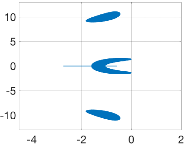
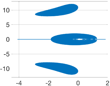
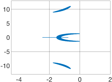
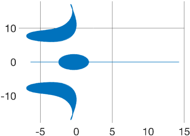
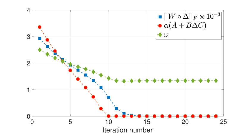
Figure 2 presents a sample run of Algorithm 1 for the case 2 of the above example. It is initialized with $\omega_{0}=2.5$ and $g_{0}=[1.0582,0.4363,1.4115,-0.0146]^{\mathsf{T}}$ and takes $24$ iterations to converge to the global minimum using the Newton descent steps. Figure 2 shows the penalized cost (scaled), spectral abscissa of the perturbed matrix $A(\Delta)$, and $\omega$ at each iteration. Observe that, at the start of the algorithm, $\alpha(A(\Delta))>0$ indicating that $A(\Delta)$ has two eigenvalues in the right-half complex plane (the other two are at $\pm j\omega$). As the iterations progress, these unstable eigenvalues move towards the left-half plane and, at the global minimum, all eigenvalues are in the closed left-half plane (c.f. discussion after (7c)). Further, the optimization cost decreases monotonically during the iterations.

Figure 2: A sample iteration run of Algorithm 1.

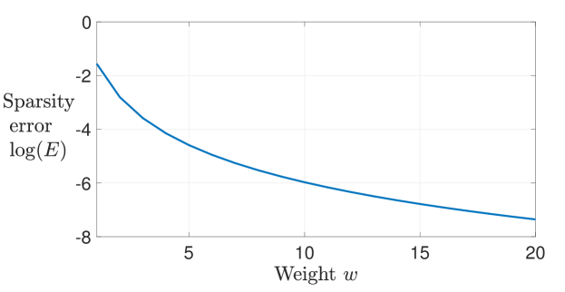
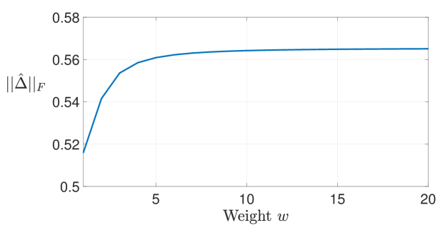
Next, we present a comparison of the global minima obtained by Algorithm 1 for different penalty weights. Table 2 shows the global minima for three values of weight ${\bf w}$. Further, Figure 3 shows the sparsity error $E\triangleq||\Delta-S\circ\Delta||_{F}$ and the norm of the optimal perturbation as a function of the weight $w$. Observe that, as the weight ${\bf w}$ increases, the sparsity error decreases and the optimal perturbations become more sparse. Furthermore, the norm of the optimal perturbations increases with ${\bf w}$, since a larger weight implies a tighter constraint on the perturbation entries.

Table 2: Approximately-sparse Solutions

${\bf w}$	$\hat{\Delta}$	$||\hat{\Delta}||_{F}$	$\hat{\omega}$
$5$	$\begin{bmatrix}-0.0414&-0.0036\\ \phantom{-}0.0095&\phantom{-}0.5593\end{bmatrix}$	$0.5609$	$1.3385$
$10$	$\begin{bmatrix}-0.0417&-0.0009\\ \phantom{-}0.0024&\phantom{-}0.5627\end{bmatrix}$	$0.5642$	$1.3370$
$20$	$\begin{bmatrix}-0.0418&-0.0002\\ \phantom{-}0.0006&\phantom{-}0.5635\end{bmatrix}$	$0.5651$	$1.3367$

Figure 3: Variation of (a) sparsity error $\log(E)$, and (b) norm of the optimal perturbation $\hat{\Delta}$, as a function of weight $w$.

(a) Line network

(b) Circular network

Figure 4: Two symmetric networks. The bold edge(s) is/are most critical and result in the smallest sparse SR.

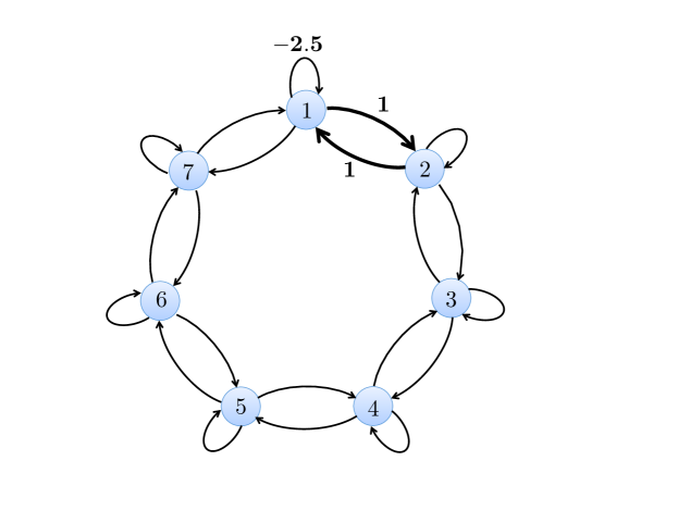
Finally, we illustrate that our sparse SR framework provides structural insights into the stability of dynamical networks. We consider symmetric line and circular networks as shown in Figure 4, where the nodes represent the scalar states and the edges represent the non-zero couplings. All self loops have weight $-2.5$ and all inter-node edges have weight $1$. The state matrix $A$ can be easily constructed using these weights and it is stable.

We are interested in identifying the edge(s) that are most critical for the stability of the network. This can be characterized by assigning a sparsity pattern corresponding to a subset of edges that are perturbed, and computing the sparse SR using the developed framework. Then, the most critical edge set is the one which results in the least SR. For the line network, we allow only a singe edge to be perturbed. It implies that only one entry of $\Delta$ is allowed to be perturbed. For the circular network, we allow for two inter-node edges to be perturbed (self loop edges are fixed). This implies that only two non-diagonal entries of $\Delta$ are allowed to be perturbed. We set $B=C=I$ for both the networks.

For the line network, we observe that the most critical edge is the self loop of the node in the center of the line (node $4$). The SR corresponding to this edge is $1.5118$. For the circular network, the two most critical inter-node edges are the edges between any two neighboring nodes. The optimal perturbations for the two edges are $0.9724$ and $0.9814$ (in any order) and the corresponding SR is $1.3816$. Due to the circular symmetry, there exist $7$ pairs of critical edges in the network. These examples highlight that our sparse SR framework is useful in studying the robust stability of sparse networks, which was not possible using the previous non-sparse SR theory.

6 Conclusion

In this paper we study the real, sparse, $F$-norm stability radius of a linear time-invariant system, which measures its ability to maintain stability in the presence of structured additive perturbations. We formulate the stability radius problem as an equality-constrained minimization problem, and characterize its optimality conditions. These conditions reveal important geometric properties of the stability radius and the associated perturbation, and allow us to design a penalty based Newton descent algorithm that provably converges to locally optimal values of the stability radius and the associated perturbation. Using the Frobenius norm to measure the size of perturbations is not only convenient for the analysis, but it also provides selective information regarding which system entries have a greater effect on system stability. Further, imposing an arbitrary sparsity pattern to the perturbation becomes crucial when studying the stability radius of network systems and, more generally, systems where only a subset of the entries can be perturbed. Numerical examples are shown to highlight the utility of our framework for characterizing structural fragility of networks.

References

- [1] D. Hinrichsen and A. J. Pritchard. Mathematical systems theory I: modeling, state space analysis, stability and robustness. Springer-Verlag Berlin Heidelberg, 2005.
- [2] D. Hinrichsen and A. J. Pritchard. Stability radii of linear systems. Systems & Control Letters, 7(1):1–10, 1986.
- [3] D. Hinrichsen and A. J. Pritchard. Stability radius for structured perturbations and the algebraic riccati equation. Systems & Control Letters, 8(2):105–113, 1986.
- [4] C. Van Loan. How near is a stable matrix to an unstable matrix. Contemporary Mathematics, 47:465–478, 1985.
- [5] R. Byers. A bisection method for measuring the distance of a stable matrix to the unstable matrices. SIAM Journal on Scientific and Statistical Computing, 9(5):875–881, 1988.
- [6] D. Hinrichsen, B. Kelb, and A. Linnemann. An algorithm for the computation of the structured complex stability radius. Automatica, 25(5):771–775, 1989.
- [7] S. Boyd, V. Balakrishnan, and P. Kabamba. A bisection method for computing the -norm of a transfer matrix and related problems. Mathematics of Control, Signals and Systems, 2(3):207–219, 1989.
- [8] S. Boyd and V. Balakrishnan. A regularity result for the singular values of a transfer matrix and a quadratically convergent algorithm for computing its -norm. Systems & Control Letters, 15(1):1–7, 1990.
- [9] N. A. Bruinsma and M. Steinbucha. A fast algorithm to compute the -norm of a transfer function matrix. Systems & Control Letters, 14(4):287–293, 1990.
- [10] L. Qiu and E. J. Davison. The stability robustness determination of state space models with real unstructured perturbations. Mathematics of Control, Signals and Systems, 4(3):447–267, 1991.
- [11] L. Qiu and E. J. Davison. Bounds on the real stability radius. In Robustness of Dynamic Systems with Parameter Uncertainties, pages 139–145, 1992.
- [12] Li Qiu, Bo Bernhardsson, Anders Rantzer, EJ Davison, PM Young, and JC Doyle. A formula for computation of the real stability radius. Automatica, 31(6):879–890, 1995.
- [13] J. Sreedhar, P. Van Dooren, and A. L. Tits. A fast algorithm to compute the real structured stability radius. Stability Theory: International Series of Numerical Mathematics, 121:219–230, 1996.
- [14] M. A. Freitag and A. Spence. A new approach for calculating the real stability radius. BIT Numerical Mathematics, 54:381–400, 2014.
- [15] N. A. Bobylev, A. V. Bulatov, and P. Diamond. An easily computable estimate for the real unstructured f-stability radius. International Journal of Control, 72(6):493–500, 1999.
- [16] N. A. Bobylev, A. V. Bulatov, and P. Diamond. Estimates of the real structured radius of stability of linear dynamic systems. Automation and Remote Control, 62(4):505–512, 2001.
- [17] N. Guglielmi and M. Manneta. Approximating real stability radii. IMA Journal of Numerical Analysis, 35(3):1402–1425, 2015.
- [18] M. W. Rostami. New algorithms for computing the real structured pseudospectral abscissa and the real stability radius of large and sparse matrices. SIAM Journal on Scientific Computing, 37(5):S447–S471, 2015.
- [19] N. Guglielmi. On the method by rostami for computing the real stability radius of large and sparse matrices. SIAM Journal on Scientific Computing, 38(3):A1662–A1681, 2016.
- [20] N. Guglielmi and C. Lubich. Low-rank dynamics for computing extremal points of real pseudospectra. SIAM Journal on Matrix Analysis and Applications, 34(1):40–66, 2013.
- [21] N Guglielmi, M. Gürbüzbalaban, T. Mitchell, and M. L. Overton. Approximating the real structured stability radius with frobenius-norm bounded perturbations. SIAM Journal on Matrix Analysis and Applications, 38(4):1323–1353, 2017.
- [22] S. C. Johnson, M. Wicks, M. Zefran, and R. A. DeCarlo. The structured distance to the nearest system without property . IEEE Transactions on Automatic Control, 63(9):2960–2975, 2018.
- [23] Petersen K. B. and M. S. Pedersen. The Matrix Cookbook. Technical University of Denmark, 2012.
- [24] J. R. Magnus and H. Neudecker. Matrix Differential Calculus with Applications in Statistics and Econometrics. John Wiley and Sons, 1999.
- [25] D. Kressner and M. Voigt. Distance problems for linear dynamical systems. In Numerical Algebra, Matrix Theory, Differential-Algebraic Equations and Control Theory, pages 559–583. Springer, 2015.
- [26] A. Hjorungnes and D. Gesbert. Complex-valued matrix differentiation: Techniques and key results. IEEE Transactions on Signal Processing, 55(6):2740––2746, 2007.
- [27] D. H. Brandwood. A complex gradient operator and its application in adaptive array theory. IEE Proceedings F - Communications, Radar and Signal Processing, 130(1):11––16, 1983.
- [28] D. G. Luenberger. Linear and Nonlinear Programming. Addison-Wesley, 2 edition, 1984.
- [29] S. P. Bhattacharyya and E. De Souza. Pole assignment via sylvester’s eqauation. Systems & Control Letters, 1(4):261––263, 1982.