A framework for algorithm deployment on cloud-based quantum computers
Abstract
In recent years, the field of quantum computing has significantly developed in both the improvement of hardware as well as the assembly of various software tools and platforms, including cloud access to quantum devices. Unfortunately, many of these resources are rapidly changing and thus lack accessibility and stability for robust algorithm prototyping and deployment. Effectively leveraging the array of hardware and software resources at a higher level, that can adapt to the rapid development of software and hardware, will allow for further advancement and democratization of quantum technologies to achieve useful computational tasks. As a way to approach this challenge, we present a flexible, high-level framework called algo2qpu that is well-suited for designing and testing instances of algorithms for near-term quantum computers on the cloud. Algorithms that employ adaptive protocols for optimizations of algorithm parameters can be grouped under the umbrella of “adaptive hybrid quantum-classical” (AHQC) algorithms. We demonstrate the utility of algo2qpu for near-term algorithm development by applying the framework to implement proof-of-principle instances of two AHQC algorithms that have applications in quantum chemistry and/or quantum machine learning, namely the quantum autoencoder and the variational quantum classifier, using Rigetti Computing’s Forest platform.
I Introduction
Significant development in both theory and experiment over the past several decades has positioned quantum computation as a promising technology for various applications, including quantum simulation Lloyd (1996); Aspuru-Guzik et al. (2005); Wecker et al. (2014); Reiher et al. (2017), discrete optimization Farhi et al. (2014); Campbell et al. (2018), and more recently, machine learning Romero et al. (2017); Wan et al. (2017); Cao et al. (2017); Farhi and Neven (2018); Schuld et al. (2018); Mitarai et al. (2018); Schuld and Killoran (2018); Huggins et al. (2018); Havlicek et al. (2018); Wilson et al. (2018). While certain quantum algorithms Shor (1994); Grover (1996); Harrow et al. (2009) guarantee speedups over their classical counterparts (e.g. Shor, Grover, HHL), useful realizations will require fault-tolerant quantum computation. Quantum devices supporting fault-tolerant quantum computation have yet to be realized. In the meantime, significant effort Peruzzo et al. (2014); Farhi et al. (2014); O’Malley et al. (2016) has been invested in leveraging the capabilities of near-term “noisy intermediate-scale quantum” (NISQ) devices that can support on the order of qubits and quantum operations Preskill (2018). From the algorithmic standpoint, NISQ devices have inspired a class of algorithms that strategically allocate computational tasks between quantum and classical resources, called hybrid quantum-classical (HQC) algorithms McClean et al. (2016). For clarity, in this work we call a subset of these HQC algorithms that use classical resources to perform optimization of algorithm parameters, adaptive hybrid quantum-classical (AHQC) algorithms111We use “adaptive” as an umbrella term to describe a group of HQC algorithms that use adaptive protocols or optimizations to update algorithm parameters. Consequently, this encompasses HQC algorithms that utilize the variational principle, such as VQE.. We show a few examples of AHQC algorithms in Table 1 that have applications in several areas including chemistry, machine learning, and factoring. Several of these AHQC algorithms, notably the variational quantum eigensolver (VQE) Peruzzo et al. (2014) and the quantum approximate optimization algorithm (QAOA) Farhi et al. (2014), have been widely studied, with the VQE algorithm demonstrated using various quantum computing architectures O’Malley et al. (2016); Kandala et al. (2017); Hempel et al. (2018). To continue and accelerate the advancement of quantum computing technologies in both theory and experiment, there is a growing need for software workflows and frameworks that enable organized, rapid testing of algorithms Zeng et al. (2017); McCaskey et al. (2018a, b).
| AHQC Algorithm | Goal(s) | Optimization Problem | ||||
|
|
Minimize expected energy | ||||
|
|
Maximize expected cut size | ||||
| Quantum Autoencoder (QAE) Romero et al. (2017) |
|
Maximize average fidelity | ||||
|
|
Maximize average fidelity | ||||
|
|
Maximize log likelihood | ||||
| Variational Quantum Factoring (VQF) Anschuetz et al. (2018) |
|
|
Fortunately, over the last few years, various academic and industrial research groups have developed an ecosystem of software tools for simulating and executing quantum circuits, as reviewed in LaRose (2018). In addition to advanced simulators, some of these platforms, including Rigetti Computing’s Forest Smith et al. (2016) and IBM’s Quantum Experience IBM , provide cloud access to their respective quantum devices. Alongside the rich suite of data tools already available in the cloud, cloud-based quantum computing is expected to become a crucial resource for both research and commercial applications Mohseni et al. (2017); Castelvecchi (2017).
Though numerous studies have already presented experimental demonstrations of quantum algorithms using cloud-based quantum computing Devitt (2016); Dumitrescu et al. (2018)222Please refer to IBM Quantum Experience’s Paper page for a comprehensive list of papers that implement experiments using IBM’s cloud service., there remains a gap between the development of an abstract algorithm and the experimental demonstration of an instance of that algorithm Chong et al. (2017). Filling in this gap is particularly important for quantum algorithms of a heuristic nature Aspuru-Guzik et al. (2005); Farhi et al. (2014); Peruzzo et al. (2014) as these algorithms rely on rapid prototyping and testing in order to fine-tune them and gauge their feasibility. Furthermore, for general quantum algorithms, significant effort is required to translate the instance of the algorithm, likely realized as abstract, noiseless quantum circuit(s) assuming all-to-all connectivity, to the corresponding lower-level quantum circuits that consider the connectivity and native gate set corresponding to actual devices. In the age of NISQ devices, this gap is compounded by the noise in the devices, prompting the need for a way to design “hardware-efficient” Kandala et al. (2017) algorithmic instances, or circuit(s) that can execute with high fidelity on a given device. Lastly, with growing efforts to build high-quality, reusable packages and platforms, development of reliable abstractions or frameworks to leverage these resources are necessary to achieve and scale up quantum computations for practical applications.
In this work, we introduce a high-level framework for prototyping and deploying AHQC algorithms, called algo2qpu, which provides a systematic workflow from abstract circuits to machine-supported gate-level circuits to execute on either an available simulator or quantum device. We developed algo2qpu with the hope of streamlining the testing of AHQC algorithms. Such testing facilitates algorithm development as well as experimental design. We note that the abstraction of algo2qpu in principle also allows for implementation of algorithms beyond AHQC algorithms, e.g. the iterative phase estimation algorithm. In the following sections, we describe algo2qpu in greater detail, present its realization using the Forest platform, and apply the infrastructure to execute proof-of-principle instances of two AHQC algorithms, the quantum autoencoder Romero et al. (2017) and the quantum variational classifier Schuld et al. (2018); Havlicek et al. (2018); Farhi and Neven (2018), on Forest’s simulator and quantum processor via the cloud.
II algo2qpu
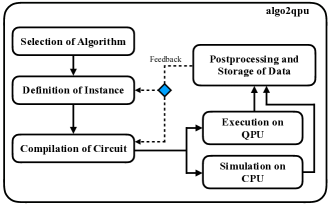
In principle, algo2qpu is a hardware and software agnostic framework well-suited for, but not limited to, implementing instances of AHQC algorithms on a quantum device. This broad framework consists of several major steps: (1) selection of an algorithm-of-interest, (2) definition of a specific instance of the algorithm, (3) compilation of the abstract quantum circuit(s) involved in the algorithmic instance, (4) execution of the compiled circuit(s) to either a simulator or a quantum device, and (5) post-processing and storage of the output data, as shown in Figure 1. In the case of AHQC algorithms, a classical feedback routine is integrated to update the algorithm parameters following an adaptive protocol.
Below we describe each step in greater detail:
1. Selection of Algorithm –
At this level, we develop and/or decide on an abstract problem or algorithm to demonstrate. In the case of many AHQC algorithms, this entails defining the objective or cost function(s) that correspond to the particular problem/task. For instance, we may choose to implement VQE, in which the main objective may be to estimate the ground state energy of a fermionic system, that is to minimize the energy of the system. Alternatively, we may be interested in implementing the quantum autoencoder to find a compressed representation of a set of quantum states, or maximizing the fidelity between the input and output data set after applying compression then recovery maps.
2. Definition of Instance – After selecting an algorithm, we define the specific instance of the algorithm in the following step. That is, we consider the quantum circuit(s) used to compute values of the objective function(s) corresponding to the algorithm. In the context of many AHQC algorithms, this generally refers to selecting the parametrized quantum circuits.
At this stage, to consider the circuits at a high level, we label the physical qubits with variables e.g. , , etc. to indicate that the qubits of the abstract circuits have yet to be assigned to these. (For an example of two instances of a particular algorithm, see Figure 4b).
3. Compilation of Abstract Circuits – Compilation of quantum circuits according to device specifications has been an area of research devoted to map a theoretical quantum circuit in the classroom or on paper to a “lower-level” quantum circuit whose instructions can be directly processed and executed on a quantum device Zulehner and Paler (2017); Paler et al. (2018); Häner et al. (2018); Heyfron and Campbell (2017); Nam et al. (2017); Venturelli et al. (2018); Steiger et al. (2018); Gushu et al. (2018). We note that the compilation step in the NISQ era can be roughly divided into two major subcomponents: qubit mapping and gate compilation. In addition, this is the step in the workflow that assumes knowledge of the quantum device (e.g. connectivity or single-qubit and two-qubit fidelities). We note that while compilation in today’s quantum computing may more closely resemble a simpler, high-level variant, significant effort is being devoted to advance compilation such that the process is more analogous to the compilation process for classical computers JavadiAbhari et al. (2014); Chong et al. (2017).
Prior to executing a quantum circuit on an actual device, the abstract qubits must be mapped onto the physical qubits of an actual device. This mapping procedure may be non-trivial due to the limited connectivity as well as the quality of the qubits on the processor. That is, even on a single device, there may be a range of qualities or fidelities among the qubits. For example, if the circuit-of-interest requires high quality two-qubit interactions for a subset of qubits, assigning those qubits to physical qubits with high two-qubit fidelities may become a priority in the mapping process.
In addition, the gates in abstract circuits are generally non-native to a particular device. For example, common gates such as CNOT or Hadamard operations are not native to several existing devices and must be decomposed in terms of the native gates of the chosen platform. We note that several existing compilation routines can also provide valuable circuit information or resource estimates, such as the circuit depth. Depending on the capabilities of the hardware-of-choice, at this stage, one may choose to re-design the experiment to work within the limitations. At the end of the compilation step of algo2qpu, the circuits are ready for execution on a simulator or a quantum device.
While our demonstrations will implement the mapping procedure before the gate compilation, we note that a deeper investigation is necessary to determine the effective ordering of these protocols that correspond to the optimal compilation of the circuit(s).
4. Circuit Simulation/Execution – Once the quantum circuits are compiled according to the hardware specifications, they can be executed on either a simulator or an actual quantum device (also called the quantum processing unit or QPU) through the cloud. In addition to a wide array of available circuit simulators (e.g. Cirq, QISKit, pyQuil, ProjectQ) Cir ; Qis (2018); Smith et al. (2016); Steiger et al. (2016), some with noise-simulating capabilities, various platforms for cloud-based quantum computing have also been integrated (e.g. Forest and IBM Quantum Experience).
Circuit executions on these services will generally output a collection of measurement outcomes, which can then be post-processed in the following step of algo2qpu.
5. Postprocessing and Storage – The post-processing routine in the framework is responsible for gathering the measurement outcomes and computing the values of the algorithm instance’s objective function(s). For NISQ devices, post-processing may significantly benefit from additional error mitigation routines Endo et al. (2018); Temme et al. (2017); McClean et al. (2017); Kandala et al. (2018). Both the raw and processed outcome information can also be stored in this step for verifiability.
6. Classical Feedback – For AHQC algorithms, the optimization of algorithm parameters is offloaded to the classical computer. In the context of algo2qpu, once the parameters have been updated by the classical optimizer, they can be updated at the level of the abstract circuit or the compiled circuit that employs parametric variables. Figure 1 illustrates the possibility of creating a new abstract circuit or directly adjusting the parameters in a compiled circuit in the classical feedback process.
Then, the re-compiled circuit is executed on the simulator or device until the convergence criteria of the AHQC algorithm are satisfied.
We note that the abstractness and modularity in the framework in principle can allow for the use of different modules and routines to implement the different steps of algo2qpu, based on the advantages of particular software packages or the availability of specific features. For example, one may use Forest’s connections to the simulator and hardware while using ProjectQ’s generalized routine for circuit compilation. In addition, depending on the available features of a platform, algo2qpu can be further optimized to reduce latency by executing certain modules, such as compilation and/or execution, locally or remotely (through the cloud) Smith et al. (2016). In the following section, we present one possible realization of the algo2qpu framework, implemented using features and services supported by the Forest platform333The version of pyQuil used for the study is 1.9.0..

III Implementation of algo2qpu using Forest
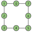
To demonstrate the utility of the algo2qpu framework, we construct each step of the workflow using various modules and/or routines available within the Forest platform, as shown in Figure 2. The choice of algorithm and its instance can be realized by either choosing an algorithmic implementation from grove, Rigetti Computing’s library of quantum algorithms, or writing a code using pyQuil that implements an algorithm, such as Sim et al. (2018). The circuit(s) used in the algorithm are represented as instances of Program that employ QubitPlaceholder to label abstract qubits, which can later be replaced with physical qubit indices. The circuit(s) can be compiled using Forest’s in-house compiler that considers the specifications of the particular quantum device. At the time of developing algo2qpu, the available quantum device was Rigetti Computing’s eight-qubit processor, 8Q-Agave, its layout shown in Figure 3. Once compiled, the circuit(s) can be executed by connecting to the device and submitting circuit jobs to the cloud, specifically to the quantum virtual machine (QVM) for simulations and the quantum processing unit (QPU) for experiments. The measurement outcomes of both the QVM and QPU are returned as a Python list, which can be post-processed to compute the algorithm’s objective(s) and then be stored using the json module. For a demonstration of the algo2qpu workflow in the context of implementing a specific algorithm, the reader should refer to Sim et al. (2018).
In the following sections, we demonstrate the Forest-implemented algo2qpu workflow to design and execute simple instances of two AHQC algorithms: the quantum autoencoder and the variational quantum classifier. For each algorithm, we provide (1) a general description of the algorithm, (2) specific instance(s) of the algorithm, followed by (3) demonstrations and analyses of these instances enabled by algo2qpu.
IV Algorithm: Quantum Autoencoder
In this section, we demonstrate simple instances of the quantum autoencoder based on a model proposed by a previous work Romero et al. (2017). Using algo2qpu, we extend this study by investigating two alternative autoencoder training schemes and providing the first experimental demonstrations of this model on the 8Q-Agave chip.
IV.1 Brief Background
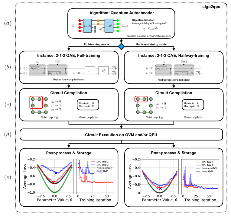
The quantum autoencoder (QAE) algorithm has been proposed in recent years Romero et al. (2017); Wan et al. (2017) as a paradigm for compressing quantum data, that is expressing a data set comprised of quantum states using a fewer number of qubits. The QAE is constructed using the following: a set of quantum states of size qubits with denoting the training set index, a choice of “trash” state of size qubits, “refresh” qubits for the recovery process, and a variational circuit () with circuit parameters for encoding (decoding), as illustrated in Figure 4a. In practice, the training set for the QAE has to be prepared on the quantum register using a corresponding set of preparation circuits such that . A successful training of the autoencoder implies finding the parameters that are able to optimally or near optimally factorize all the states in the training set as follows:
| (1) |
where is the compressed representation (on only qubits) of . We can then faithfully recover the input state after applying the decoding operation on the state , where is prepared on the “refresh” qubits. Consequently, these capabilities may be useful for applications such as dimension reduction of quantum and classical data and feature extraction.
When implementing the autoencoder, we can choose various types of cost functions. In this work, we modify the original autoencoder protocol to accommodate the limitations of the quantum device, avoiding the need for implementing SWAP tests. We first consider a cost function that is computed by executing the full QAE circuit, including, in order, the state preparation, encoding, decoding, and inversed state preparation circuit components. In this case, the success probability of the autoencoder corresponds to the probability of measuring the state at the end of the circuit. In our implementation, we negate this probability value to cast as a minimization problem and average the frequencies over the training set to compute a single loss value. We will refer to this cost function as “full-training”. Alternatively, we can consider computing the average probability of measuring the state in the trash register after applying the encoding variational circuit. Similarly, we average over the training set to compute a single loss value. We will refer to this second cost function as “halfway-training.”
IV.2 Algorithmic Instance: 2-1-2 Autoencoder
To demonstrate our use of the algo2qpu framework for the quantum autoencoder, we consider a simple 2-1-2 instance using both the “full” and “halfway” autoencoder training schemes, as shown in the left and right panels of Figure 4b. Our data set is composed of two-qubit states, generated by considering a range of values in the state preparation circuit, shown in Figure 4b, in this case forty equally-spaced points from 0 to , and the objective is to compress the information such that we can express the input data set using a single qubit. Eight randomly selected points in the data set were selected as the training set. Our simple example is devised such that when the single variational parameter is , this corresponds to the ideal two-to-one compression circuit. We use the notation to refer to qubit indexes in the “abstract” QAE circuits in Figure 4b, to anticipate the potentially nontrivial mapping of abstract qubits to physical qubits when implementing the circuit on an actual quantum device with specific connectivity.
IV.3 Circuit Compilation
Based on the single- and two- qubit fidelities during the times of the experiments, physical qubits 0, 1, and 2 were selected for the full training scheme, and physical qubits 0 and 1 were selected for the halfway training scheme, with trivial mappings for both cases as shown in Figure 4c. We note that while this selection was done manually for the example in this paper, general workflows will involve automated protocols for qubit mapping. Some examples of these protocols are presented in Paler et al. (2018); Zulehner and Paler (2017). After scanning over values for , fifty equally-spaced points from to , we also report the minimum and maximum gate depths for each training scheme in Figure 4c. The gate compilation step was performed using the software tools available in the Forest platform Smith et al. (2016).
| Setting |
|
|
||||
|---|---|---|---|---|---|---|
| Full, QPU (Trial 1) | -0.76 0.03 | -0.75 0.02 | ||||
| Full, QPU (Trial 2) | -0.53 0.05 | -0.44 0.06 | ||||
| Halfway, QPU (Trial 1) | -0.874 0.002 | -0.875 0.002 | ||||
| Halfway, QPU (Trial 2) | -0.90 0.02 | -0.84 0.03 |
IV.4 Simulation and Experimental Results
Numerical simulations and experiments of the quantum autoencoder for this study were implemented and executed using an extended version of the QCompress code Sim et al. (2018). For both training schemes, each cost function value was evaluated by taking 10000 circuit runs per data point in the training set. For optimizing the variational parameter , the COBYLA algorithm was used, with the initial value of set randomly to for all experiments. A parameter sweep for was performed, computing the cost function landscape for fifty equally-spaced points, to assess the impact of experimental conditions on the average loss and on the overall algorithmic performance before each parameter optimization. Two experimental trials were executed for each training scheme, complemented by simulation data 444Tomography experiments are periodically executed by Rigetti Computing to construct a device-imitating noise model for the noisy variant of Forest’s circuit simulator.. To evaluate the performance of the autoencoder, we compute the loss values against a test set, which we have pre-selected when randomly splitting the full data set into training and test sets (eight and thirty-two data points respectively).
As shown in Figure 4e, we observe decays in the average loss values for the cost function landscapes of the full and halfway training cases, but the quantum autoencoder was able to reach close to the optimal parameter value of 0 despite the noise in the quantum computer. We also point out that the two executions of the QPU corresponding to full training were performed on different days, and therefore the significant difference might be associated to different calibrations. As expected, due to shorter circuit depths, the cost function landscapes for the halfway training cases better align with results from noisy simulations. In addition, the halfway training scheme produced better average loss values for both training and test sets, as shown in Table 2. This appears to suggest that the halfway training scheme may be a promising alternative and should be further explored with larger instances of the algorithm as a viable training technique for the quantum autoencoder.
V Algorithm: Variational Quantum Classifier
Here we demonstrate a simple example of a variational quantum classifier in full implementation details. The goal here is to provide a minimal example that introduces step by step the workflow of realizing variational quantum classifiers on quantum devices.
V.1 Brief Background
There has been a rapidly growing set of works in the past few months on using near-term quantum computers for classification problems in machine learning Farhi and Neven (2018); Schuld et al. (2018); Huggins et al. (2018); Wilson et al. (2018); Havlicek et al. (2018); Schuld and Killoran (2018); Mitarai et al. (2018). Here we consider the problem of binary classification i.e. learning a function . One of the prevalent methodologies is to variationally tune a quantum circuit and use the measurement outcomes to obtain the output label generated by the quantum model Farhi and Neven (2018); Schuld et al. (2018); Huggins et al. (2018); Wilson et al. (2018); Havlicek et al. (2018). For a given training set where consists of all data points labeled 0 and labeled 1, one optimizes the circuit parameter such that for all inputs in the quantum model returns 0 as much as possible and for the model returns 1 as much as possible. There are also alternative proposals for quantum classifiers based on kernel space Schuld and Killoran (2018); Havlicek et al. (2018). However, here we focus on the variational classifier model.
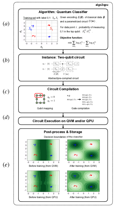
To implement a variational quantum classifier, one immediate question is how the quantum computer interacts with the classical world. The present literature has more or less reached a consensus on this being a four-part process: (1) encode a classical input vector into a quantum state , (2) apply a variational circuit of parameters onto the encoded state, (3) collect measurement statistics of the final state with respect to some operator , (4) classically postprocess the measurement outcomes to obtain the output label of the quantum model. Different proposals Farhi and Neven (2018); Schuld et al. (2018); Huggins et al. (2018); Wilson et al. (2018); Havlicek et al. (2018) use different choices for each step, while the overall framework remains largely the same. Here we also adopt this framework in our example.
V.2 Algorithmic Instance: Learning XOR
For a set of data points , , in dimensional space, the simplest model for classifying the data points is a linear function . Depending on whether the value of the function is above or below a predefined threshold we apply a discrete label to the data point . That is, we are essentially using a hyperplane to separate the data points. The set of such that therefore forms a decision boundary where is applied one label if i.e. it lies on one side of the decision boundary and another label if i.e. it lies on the other side of the decision boundary.
If the data points are not linearly separable, then we need to use a different form of which generates nonlinear boundaries. A classic example of linearly inseparable data is the “XOR” dataset555Historically this is a famed example showing the limitation of perceptrons proposed by Minsky and Papert Minsky and Papert (1969). The fact that XOR functions can be learned by multilayer perceptrons was only widely recognized later. (Figure 5b). Here we specifically consider an XOR-like training set with being points around , and being points around .
To encode a classical input , we use the encoding by preparing a quantum state , where is a single qubit rotation along the direction. Similar ideas for encoding classical data have been proposed before Huggins et al. (2018), though in general a more compact encoding is possible Mitarai et al. (2018); Schuld et al. (2018). We then apply a parametrized unitary and measure the top qubit. We will use the probability of measuring in the top qubit as the output label (as also considered in Farhi and Neven (2018)). The objective function that we would like to minimize is the cross entropy
| (2) |
In other words, we want to maximize the output (and therefore ) when the data label is 1 and at the same time minimize the output when the data label is 0.
V.3 Simulation and Experimental Results
We start from an initial guess of the parameter that does not give rise to good classification (Figure 5c) and optimize the circuit parameters using Nelder-Mead. The trained classifier captures closer the XOR function (Figure 5d).
Observe that in fact the parameter does not enter in the objective function, rendering the optimization problem as essentially one-dimensional. One could in fact absorb the gate into the measurement of the bottom qubit, and treat as a parameter setting the measurement context only for the bottom qubit. This way the value of does not influence the measurement outcome on the top qubit. We can see this also by explicitly computing the probability :
| (3) |
From the above expression it is clear that the term naturally gives rise to the XOR-like landscape in Figure 5d by assigning different signs to its extrema according to the quadrant. The optimal parameter setting is then , which gives a that contains only the desired term.
Finally we remark that the observation that the circuit in Figure 5b can be effective in partitioning the XOR data comes from iterative trial and error within the algo2qpu framework. Initially, the circuit is trained to classify an XOR-shaped data set similar to Figure 5b but shifted, with being points around and around . From plotting the decision boundary of the optimized circuit (similar to Figure 5e) we observe that although the circuit classifies the original XOR data set poorly, it perfectly classifies a shifted version of the data described (Figure 5a). This shows that we can learn new information by actually running the circuit (either on hardware or on simulator) and these new information can help us improve the use of quantum circuits.
VI Discussion and Conclusion
With steady improvement of quantum hardware, coupled with developments in various software packages and cloud access to quantum processors, we are becoming better-equipped to test small instances of algorithms and perform important benchmark studies, ultimately to anticipate and prepare tasks for large-scale error-corrected quantum computers. In this paper, we have introduced a modular framework to guide and streamline the prototyping process for AHQC algorithms and demonstrated its use in designing and executing experiments by leveraging cloud access to quantum processors. Changes and improvements in each component of algo2qpu will, in principle, benefit the overall framework and yield a better pipeline for demonstrating the utility of quantum devices.666We note that Rigetti Computing has recently released an update to its platform, called the Quantum Cloud Services. Despite the changes, major steps of algo2qpu can still be applied and implemented using the updated code and service. While the current framework refers to adapting circuits, e.g. directly tuning the gate parameters, one could imagine improving and extending this framework to adaptively adjust parameters of higher-level processes or routines which implicitly involve lower-level quantum circuits. Nevertheless, continuing the efforts to build similar frameworks will enable efficient algorithmic testing that can eventually scale up to larger experiments and also provide a testbed for developing new and exploratory classes of algorithms, such as HQC algorithms in quantum machine learning. Just as AHQC algorithms were intended to make the most out of existing hardware, developing and/or formalizing software infrastructures that can unify multiple platforms, such as algo2qpu, will allow us to leverage capabilities of existing or near-term quantum software and hardware, setting the stage for more practical and powerful quantum computations.
Acknowledgements.
We thank Rigetti Computing for providing access to their quantum computer. We especially thank Ryan Karle for his help in setting up and running jobs on the 8Q-Agave device. The views expressed in this paper are those of the authors and do not reflect those of Rigetti Computing. We also thank Jonathan Olson, Morten Kjaergaard, Max Radin, and Timothy Hirzel for helpful discussions and comments on the manuscript. S. S. is supported by the DOE Computational Science Graduate Fellowship under grant number DE-FG02-97ER25308.References
- Lloyd (1996) S. Lloyd, Science 273, 1073 (1996).
- Aspuru-Guzik et al. (2005) A. Aspuru-Guzik, A. D. Dutoi, P. J. Love, and M. Head-Gordon, Science 309, 1704 (2005).
- Wecker et al. (2014) D. Wecker, B. Bauer, B. K. Clark, M. B. Hastings, and M. Troyer, Phys. Rev. A 90, 022305 (2014).
- Reiher et al. (2017) M. Reiher, N. Wiebe, K. M. Svore, D. Wecker, and M. Troyer, Proc. Natl. Acad. Sci. , 7555 (2017).
- Farhi et al. (2014) E. Farhi, J. Goldstone, and S. Gutmann, (2014), arXiv:1411.4028 .
- Campbell et al. (2018) E. Campbell, A. Khurana, and A. Montanaro, (2018), arXiv:1810.05582 .
- Romero et al. (2017) J. Romero, J. P. Olson, and A. Aspuru-Guzik, Quantum Sci. Technol. 2, 045001 (2017).
- Wan et al. (2017) K. H. Wan, O. Dahlsten, H. Kristjánsson, R. Gardner, and M. S. Kim, npj Quantum Information 3, 36 (2017).
- Cao et al. (2017) Y. Cao, G. G. Guerreschi, and A. Aspuru-Guzik, (2017), arXiv:1711.11240 .
- Farhi and Neven (2018) E. Farhi and H. Neven, (2018), arXiv:1802.06002 .
- Schuld et al. (2018) M. Schuld, A. Bocharov, K. Svore, and N. Wiebe, (2018), arXiv:1804.00633 .
- Mitarai et al. (2018) K. Mitarai, M. Negoro, M. Kitagawa, and K. Fujii, (2018), arXiv:1803.00745 .
- Schuld and Killoran (2018) M. Schuld and N. Killoran, (2018), arXiv:1803.07128 .
- Huggins et al. (2018) W. Huggins, P. Patel, K. B. Whaley, and E. M. Stoudenmire, (2018), arXiv:1803.11537 .
- Havlicek et al. (2018) V. Havlicek, A. D. Córcoles, K. Temme, A. W. Harrow, A. Kandala, J. M. Chow, and J. M. Gambetta, (2018), arXiv:1804.11326 .
- Wilson et al. (2018) C. M. Wilson, J. S. Otterbach, N. Tezak, R. S. Smith, G. E. Crooks, and M. P. da Silva, (2018), arXiv:1806.08321 .
- Shor (1994) P. Shor, in Proceedings 35th Annual Symposium on Foundations of Computer Science (IEEE Comput. Soc. Press, 1994).
- Grover (1996) L. K. Grover, in Proceedings of the twenty-eighth annual ACM symposium on Theory of computing - STOC ’96 (ACM Press, 1996).
- Harrow et al. (2009) A. W. Harrow, A. Hassidim, and S. Lloyd, Phys. Rev. Lett. 103, 150502 (2009).
- Peruzzo et al. (2014) A. Peruzzo, J. McClean, P. Shadbolt, M.-H. Yung, X.-Q. Zhou, P. J. Love, A. Aspuru-Guzik, and J. L. O’Brien, Nat. Commun. 5, 4213 (2014).
- O’Malley et al. (2016) P. O’Malley, R. Babbush, I. Kivlichan, J. Romero, J. McClean, R. Barends, J. Kelly, P. Roushan, A. Tranter, N. Ding, B. Campbell, Y. Chen, Z. Chen, B. Chiaro, A. Dunsworth, A. Fowler, E. Jeffrey, E. Lucero, A. Megrant, J. Mutus, M. Neeley, C. Neill, C. Quintana, D. Sank, A. Vainsencher, J. Wenner, T. White, P. Coveney, P. Love, H. Neven, A. Aspuru-Guzik, and J. Martinis, Phys. Rev. X 6, 031007 (2016).
- Preskill (2018) J. Preskill, Quantum 2, 79 (2018).
- McClean et al. (2016) J. R. McClean, J. Romero, R. Babbush, and A. Aspuru-Guzik, New J. Phys. 18, 023023 (2016).
- Kandala et al. (2017) A. Kandala, A. Mezzacapo, K. Temme, M. Takita, M. Brink, J. M. Chow, and J. M. Gambetta, Nature 549, 242 (2017).
- Hempel et al. (2018) C. Hempel, C. Maier, J. Romero, J. McClean, T. Monz, H. Shen, P. Jurcevic, B. P. Lanyon, P. Love, R. Babbush, A. Aspuru-Guzik, R. Blatt, and C. F. Roos, Phys. Rev. X 8, 031022 (2018).
- Zeng et al. (2017) W. Zeng, B. Johnson, R. Smith, N. Rubin, M. Reagor, C. Ryan, and C. Rigetti, Nature 549, 149 (2017).
- McCaskey et al. (2018a) A. McCaskey, E. Dumitrescu, D. Liakh, and T. Humble, (2018a), arXiv:1805.09279 .
- McCaskey et al. (2018b) A. McCaskey, E. Dumitrescu, D. Liakh, M. Chen, W. Feng, and T. Humble, SoftwareX 7, 245 (2018b).
- Johnson et al. (2017) P. D. Johnson, J. Romero, J. Olson, Y. Cao, and A. Aspuru-Guzik, (2017), arXiv:1711.02249 .
- Anschuetz et al. (2018) E. R. Anschuetz, J. P. Olson, A. Aspuru-Guzik, and Y. Cao, (2018), arXiv:1808.08927 .
- LaRose (2018) R. LaRose, (2018), arXiv:1807.02500 .
- Smith et al. (2016) R. S. Smith, M. J. Curtis, and W. J. Zeng, (2016), arXiv:1608.03355 .
- (33) “IBM Quantum Experience,” https://www.research.ibm.com/ibm-q/.
- Mohseni et al. (2017) M. Mohseni, P. Read, H. Neven, S. Boixo, V. Denchev, R. Babbush, A. Fowler, V. Smelyanskiy, and J. Martinis, Nature 543, 171 (2017).
- Castelvecchi (2017) D. Castelvecchi, Nature 543, 159 (2017).
- Devitt (2016) S. J. Devitt, Phys. Rev. A 94, 032329 (2016).
- Dumitrescu et al. (2018) E. F. Dumitrescu, A. J. McCaskey, G. Hagen, G. R. Jansen, T. D. Morris, T. Papenbrock, R. C. Pooser, D. J. Dean, and P. Lougovski, Phys. Rev. Lett. 120, 210501 (2018).
- Chong et al. (2017) F. T. Chong, D. Franklin, and M. Martonosi, Nature 549, 180 (2017).
- Zulehner and Paler (2017) A. Zulehner and A. Paler, (2017), arXiv:1712.04722 .
- Paler et al. (2018) A. Paler, A. Zulehner, and R. Wille, (2018), arXiv:1806.07241 .
- Häner et al. (2018) T. Häner, D. S. Steiger, K. Svore, and M. Troyer, Quantum Sci. Technol. 3, 020501 (2018).
- Heyfron and Campbell (2017) L. Heyfron and E. T. Campbell, (2017), arXiv:1712.01557 .
- Nam et al. (2017) Y. Nam, N. J. Ross, Y. Su, A. M. Childs, and D. Maslov, npj Quantum Information 4, 23 (2017).
- Venturelli et al. (2018) D. Venturelli, M. Do, E. Rieffel, and J. Frank, Quantum Sci. Technol. 3, 025004 (2018).
- Steiger et al. (2018) D. S. Steiger, T. Häner, and M. Troyer, (2018), arXiv:1806.01861 .
- Gushu et al. (2018) Gushu, Y. Ding, and Y. Xie, (2018), arXiv:1809.02573 .
- JavadiAbhari et al. (2014) A. JavadiAbhari, S. Patil, D. Kudrow, J. Heckey, A. Lvov, F. T. Chong, and M. Martonosi, Proceedings of the 11th ACM Conference on Computing Frontiers - CF ’14 , 1 (2014).
- (48) “Cirq,” https://github.com/quantumlib/Cirq.
- Qis (2018) “Quantum Information Software Kit (QISKit),” https://qiskit.org/ (2018).
- Steiger et al. (2016) D. S. Steiger, T. Häner, and M. Troyer, Quantum 2, 49 (2016).
- Endo et al. (2018) S. Endo, S. C. Benjamin, and Y. Li, Phys. Rev. X 8, 031027 (2018).
- Temme et al. (2017) K. Temme, S. Bravyi, and J. M. Gambetta, Phys. Rev. Lett. 119, 180509 (2017).
- McClean et al. (2017) J. R. McClean, M. E. Kimchi-Schwartz, J. Carter, and W. A. de Jong, Phys. Rev. A 95, 042308 (2017).
- Kandala et al. (2018) A. Kandala, K. Temme, A. D. Corcoles, A. Mezzacapo, J. M. Chow, and J. M. Gambetta, (2018), arXiv:1805.04492 .
- Sim et al. (2018) S. Sim, E. Anderson, E. Brown, and J. Romero, “QCompress: Quantum Autoencoder Implementation using Forest and OpenFermion,” https://github.com/hsim13372/QCompress (2018).
- Minsky and Papert (1969) M. Minsky and S. Papert, The MIT Press, Cambridge, expanded edition (1969).