Efficient leave-one-out cross-validation for Bayesian non-factorized normal and Student-$t$ models

Abstract

Cross-validation can be used to measure a model’s predictive accuracy for the purpose of model comparison, averaging, or selection. Standard leave-one-out cross-validation (LOO-CV) requires that the observation model can be factorized into simple terms, but a lot of important models in temporal and spatial statistics do not have this property or are inefficient or unstable when forced into a factorized form. We derive how to efficiently compute and validate both exact and approximate LOO-CV for any Bayesian non-factorized model with a multivariate normal or Student-$t$ distribution on the outcome values. We demonstrate the method using lagged simultaneously autoregressive (SAR) models as a case study. Keywords: cross-validation, Pareto-smoothed importance-sampling, non-factorized models, Bayesian inference, SAR models

1 Introduction

In the absence of new data, cross-validation is a general approach for evaluating a statistical model’s predictive accuracy for the purpose of model comparison, averaging, or selection (Geisser and Eddy,, 1979; Hoeting et al.,, 1999; Ando and Tsay,, 2010; Vehtari and Ojanen,, 2012). One widely used variant of cross-validation is leave-one-out cross-validation (LOO-CV), where observations are left out one at a time and then predicted based on the model fit to the remaining data. Predictive accuracy is evaluated by first computing a pointwise predictive measure and then taking the sum of these values over all observations to obtain a single measure of predictive accuracy (e.g., Vehtari et al.,, 2017). In this paper, we focus on the expected log predictive density (ELPD) as the measure of predictive accuracy. The ELPD takes the whole predictive distribution into account and is less focused on the bulk of the distribution compared to other common measures such as the root mean squared error (RMSE) or mean absolute error (MAE; see Vehtari and Ojanen,, 2012, for details). Exact LOO-CV is costly, as it requires fitting the model as many times as there are observations in the data. Depending on the size of the data, complexity of the model, and estimation method, this can be practically infeasible as it simply requires too much computation time. For this reason, fast approximate versions of LOO-CV have been developed (Gelfand et al.,, 1992, Vehtari et al., (2017)), most recently using Pareto-smoothed importance-sampling (PSIS; Vehtari et al.,, 2017, 2019).

A standard assumption of any such fast LOO-CV approach using the ELPD is that the model over all observations has to have a factorized form. That is, the overall observation model should be represented as the product of the pointwise models for each observation. However, many important models do not have this factorization property. Particularly in temporal and spatial statistics it is common to fit multivariate normal or Student-$t$ models that have structured covariance matrices such that the model does not factorize. This is typically due to the fact that observations depend on other observations from different time periods or different spatial units in addition to the dependence on the model parameters. Some of these models are actually non-factorizable, that is, we do not know of any reformulation that converts the observation model into a factorized form. Other non-factorized models could be factorized in theory but it is sometimes more robust or efficient to marginalize out certain parameters, for instance observation-specific latent variables, and then work with a non-factorized model instead.

Conceptually, a factorized model is not required for cross-validation in general or LOO-CV in particular to make sense. This also implies that neither conditional independence nor conditional exchangability are necessary assumptions. However, when using non-factorized observation models in LOO-CV, computational challenges arise. In this paper, we derive how to perform efficient approximate LOO-CV for any Bayesian multivariate normal or Student-$t$ model with an invertible covariance or scale matrix, regardless of whether or not the model factorizes. We also provide equations for computing exact LOO-CV for these models, which can be used to validate the approximation and to handle problematic observations. Throughout, a Bayesian model specification and estimation via Markov chain Monte Carlo (MCMC) is assumed. We have implemented the developed methods in the R package brms (Bürkner,, 2017, 2018). All materials including R source code are available in an online supplement.

2 Pointwise log-likelihood for non-factorized models

When computing ELPD-based exact LOO-CV for a Bayesian model we need to compute the log leave-one-out predictive densities $\log{p(y_{i}|y_{-i})}$ for every response value $y_{i},\>i=1,\ldots,N$, where $y_{-i}$ denotes all response values except observation $i$. To obtain $p(y_{i}|y_{-i})$, we need to have access to the pointwise likelihood $p(y_{i}\,|\,y_{-i},\theta)$ and integrate over the model parameters $\theta$:

$$p(y_{i}\,|\,y_{-i})=\int p(y_{i}\,|\,y_{-i},\theta)\,p(\theta\,|\,y_{-i})\,d\theta$$ (1)

Here, $p(\theta\,|\,y_{-i})$ is the leave-one-out posterior distribution for $\theta$, that is, the posterior distribution for $\theta$ obtained by fitting the model while holding out the $i$th observation (in Section 3, we will show how refitting the model to data $y_{-i}$ can be avoided).

If the observation model is formulated directly as the product of the pointwise observation models, we call it a factorized model. In this case, the likelihood is also the product of the pointwise likelihood contributions $p(y_{i}\,|\,y_{-i},\theta)$. To better illustrate possible structures of the observation models, we formally divide $\theta$ into two parts, observation-specific latent variables $f=(f_{1},\ldots,f_{N})$ and hyperparameters $\psi$, so that $p(y_{i}\,|\,y_{-i},\theta)=p(y_{i}\,|\,y_{-i},f_{i},\psi)$. Depending on the model, one of the two parts of $\theta$ may also be empty. In very simple models, such as linear regression models, latent variables are not explicitely presented and response values are conditionally independent given $\psi$, so that $p(y_{i}\,|\,y_{-i},f_{i},\psi)=p(y_{i}\,|\,\psi)$ (see Figure 1 (a)). The full likelihood can then be written in the familiar form

$$p(y\,|\,\psi)=\prod_{i=1}^{N}p(y_{i}\,|\,\psi),$$ (2)

where $y=(y_{1},\ldots,y_{N})$ denotes the vector of all responses. When the likelihood factorizes this way, the conditional pointwise log-likelihood can be obtained easily by computing $p(y_{i}\,|\,\psi)$ for each $i$ with computational cost $O(n)$.

If directional paths between consecutive responses are added, responses are no longer conditionally independent, but the model factorizes to simple terms with Markovian dependency. This is common in time-series models. For example, in an autoregressive model of order 1 (see Figure 1 (b)), the pointwise likelihoods are given by $p(y_{i}\,|\,y_{i-1},\psi)$. In other time series, models may have observation-specific latent variables $f_{i}$ and conditionally independent responses so that the pointwise log-likelihoods simplify to $p(y_{i}\,|\,y_{-i},f_{i},\psi)=p(y_{i}\,|\,f_{i})$. In models without directional paths between the latent values $f$ (see Figure 1 (c)), such as latent Gaussian processes (GPs; e.g., Rasmussen,, 2003) or spatial conditional autoregressive (CAR) models (e.g., Gelfand and Vounatsou,, 2003), an explicit joint prior over $f$ is imposed. In models with directional paths between the latent values $f$ (see Figure 1 (d)), such as hidden Markov models (HMMs; e.g., Rabiner and Juang,, 1986), the joint prior over $f$ is defined implicitly via the directional dependencies. What is more, estimation can make use of the latent Markov property of such models, for example, using the Kalman filter (e.g., Welch et al.,, 1995). In all of these cases (i.e., Figure 1 (a) to (d)), the factorization property is retained and computational cost for the pointwise log-likelihood contributions remains in $O(n)$.

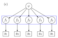
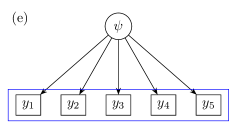
Figure 1: Directional graphs illustrating common observation model dependency structures schematically. Black rectangles depict manifest variables, that is, observed response values. Black circles depict latent variables and parameters. Blue rectangles indicate a joint prior over the surrounded variables. (a) Conditionally independent responses given hyperparameters (e.g., a linear regression model). (b) Conditionally dependent responses with a Markovian property (e.g., an autoregressive model of order 1). (c) Conditionally independent responses given observation-specific latent variables with a joint prior (e.g., a latent Gaussian process model). (d) Conditionally independent responses given observation-specific latent variables with a Markov property (e.g., a hidden Markov model). (e) Non-factorized model with a joint observation model over all responses.

Yet, there are several reasons why a non-factorized observation model (see Figure 1 (e)) may be necessary or preferred. In non-factorized models, the joint likelihood of the response values $p(y\,|\,\theta)$ is not factorized into observation-specific components, but rather given directly as one joint expression. For some models, an analytical factorized formulation is simply not available in which case we speak of a non-factorizable model. Even in models whose observation model can be factorized in principle, it may still be preferable to use a non-factorized form. This is true in particular for models with observation-specific latent variables (see Figure 1 (c) and (d)), as a non-factorized formulation where the latent variables have been integrated out is often more efficient and numerically stable. For example, a latent GP combined with a Gaussian observation model can be fit more efficiently by marginalizing over $f$ and formulating the GP directly on the responses $y$ (e.g., Rasmussen,, 2003). Such marginalization has the additional advantage that both exact and approximate leave-one-out predictive estimation become more stable. This is because, in the factorized formulation, leaving out response $y_{i}$ also implies treating the corresponding latent variable $f_{i}$ as missing, which is then only identified through the joint prior over $f$. If this prior is weak, the posterior of $f_{i}$ is highly influenced by one observation and the leave-one-out predictions of $y_{i}$ may be unstable both numerically and because of estimation error due to finite MCMC sampling or similar finite approximations.

Whether a non-factorized model is used by necessity or for efficiency and stability, it comes at the cost of having no direct access to the leave-one-out predictive densities (1) and thus to the overall leave-one-out predictive accuracy. In theory, we can express the observation-specific likelihoods in terms of the joint likelihood via

$$p(y_{i}\,|\,y_{i-1},\theta)=\frac{p(y\,|\,\theta)}{p(y_{-i}\,|\,\theta)}=\frac{p(y\,|\,\theta)}{\int p(y\,|\,\theta)\,dy_{i}},$$ (3)

but the expression on the right-hand side of (3) may not always have an analytical solution. Computing $\log p(y_{i}\,|\,y_{-i},\theta)$ for non-factorized models is therefore often impossible, or at least inefficient and numerically unstable. However, there is a large class of multivariate normal and Student-$t$ models for which we will provide efficient analytical solutions in this paper.

2.1 Non-factorized normal models

The density of the $N$ dimensional multivariate normal distribution of vector $y$ is given by

$$p(y|\mu,\Sigma)=\frac{1}{\sqrt{(2\pi)^{N}|\Sigma|}}\exp\left(-\frac{1}{2}(y-\mu)^{\rm T}\Sigma^{-1}(y-\mu)\right)$$ (4)

with mean vector $\mu$ and covariance matrix $\Sigma$. Often $\mu$ and $\Sigma$ are functions of the model parameters $\theta$, that is, $\mu=\mu(\theta)$ and $\Sigma=\Sigma(\theta)$, but for notational convenience we omit the potential dependence of $\mu$ and $\Sigma$ on $\theta$ unless it is relevant. Using standard multivariate normal theory (e.g., Tong,, 2012), we know that for the $i$th observation the conditional distribution $p(y_{i}|y_{-i},\theta)$ is univariate normal with mean

$$\tilde{\mu}_{i}=\mu_{i}+\sigma_{i,-i}\Sigma^{-1}_{-i}(y_{-i}-\mu_{-i})$$ (5)

and variance

$$\tilde{\sigma}_{i}=\sigma_{ii}+\sigma_{i,-i}\Sigma^{-1}_{-i}\sigma_{-i,i}.$$ (6)

In the equations above, $\mu_{-i}$ is the mean vector without the $i$th element, $\Sigma_{-i}$ is the covariance matrix without the $i$th row and column ($\Sigma^{-1}_{-i}$ is its inverse), $\sigma_{i,-i}$ and $\sigma_{-i,i}$ are the $i$th row and column vectors of $\Sigma$ without the $i$th element, and $\sigma_{ii}$ is the $i$th diagonal element of $\Sigma$. Equations (5) and (6) can be used to compute the pointwise log-likelihood values as

$$\log p(y_{i}\,|\,y_{-i},\theta)=-\frac{1}{2}\log(2\pi\tilde{\sigma}_{i})-\frac{1}{2}\frac{(y_{i}-\tilde{\mu}_{i})^{2}}{\tilde{\sigma}_{i}}.$$ (7)

Evaluating equation (7) for each $y_{i}$ and each posterior draw $\theta_{s}$ then constitutes the input for the LOO-CV computations. However, the resulting procedure is quite inefficient. Computation is usually dominated by the $O(N^{k})$ cost of computing $\Sigma_{-i}^{-1}$, where $k$ depends on the structure of $\Sigma$. If $\Sigma$ is dense then $k=3$. For sparse $\Sigma$ or reduced rank computations we have $2<k<3$. And since $\Sigma_{-i}^{-1}$ must be computed for each $i$, the overall complexity is actually $O(N^{k+1})$.

Additionally, if $\Sigma_{-i}$ also depends on the model parameters $\theta$ in a non-trivial manner, which is the case for most models of practical relevance, then it needs to be inverted for each of the $S$ posterior draws. Therefore, in most applications the overall complexity will actually be $O(SN^{k+1})$, which will be impractical in most situations. Accordingly, we seek to find more efficient expressions for $\tilde{\mu}_{i}$ and $\tilde{\sigma}_{i}$ that make these computations feasible in practice.

Proposition 1

If $y$ is multivariate normal with mean vector $\mu$ and covariance matrix $\Sigma$, then the conditional mean and standard deviation of $y_{i}$ given $y_{-i}$ for any observation $i$ can be computed as

$$\tilde{\mu}_{i}=y_{i}-\frac{g_{i}}{\bar{\sigma}_{ii}},$$ (8)

$$\tilde{\sigma}_{i}=\frac{1}{\bar{\sigma}_{ii}},$$ (9)

where $g_{i}=\left[\Sigma^{-1}(y-\mu)\right]_{i}$ and $\bar{\sigma}_{ii}=\left[\Sigma^{-1}\right]_{ii}$.

The proof is based on results from Sundararajan and Keerthi, (2001) and is provided in the Appendix. Contrary to the brute force computations in (5) and (6), where $\Sigma_{-i}$ has to be inverted separately for each $i$, equations (8) and (9) require inverting the full covariance matrix $\Sigma$ only once and it can be reused for each $i$. This reduces the computational cost to $O(N^{k})$ if $\Sigma$ is independent of $\theta$ and $O(SN^{k})$ otherwise. If the model is parameterized in terms of the covariance matrix $\Sigma=\Sigma(\theta)$, it is not possible to reduce the complexity further as inverting $\Sigma$ is unavoidable. However, if the model is parameterized directly through the inverse of $\Sigma$, that is $\Sigma^{-1}=\Sigma^{-1}(\theta)$, the complexity goes down to $O(SN^{2})$. Note that the latter is not possible in the brute force approach as both $\Sigma$ and $\Sigma^{-1}$ are required.

2.2 Non-factorized Student-$t$ models

Several generalizations of the multivariate normal distribution have been suggested, perhaps most notably the multivariate Student-$t$ distribution (Zellner,, 1976), which has an additional positive degrees of freedom parameter $\nu$ that controls the tails of the distribution. If $\nu$ is small, the tails are much fatter than those of the normal distribution. If $\nu$ is large, the multivariate Student-$t$ distribution becomes more similar to the corresponding multivariate normal distribution and is equal to the latter for $\nu\rightarrow\infty$. As $\nu$ can be estimated alongside the other model parameters in Student-$t$ models, the thickness of the tails is flexibly adjusted based on information from the observed response values and the prior. The (multivariate) Student-$t$ distribution has been studied in various places (e.g., Zellner,, 1976; O’Hagan,, 1979; Fernández and Steel,, 1999; Zhang and Yeung,, 2010; Piché et al.,, 2012; Shah et al.,, 2014). For example, Student-$t$ processes which are based on the multivariate Student-$t$ distribution constitute a generalization of Gaussian processes while retaining most of the latter’s favorable properties (Shah et al.,, 2014).

The density of the $N$ dimensional multivariate Student-$t$ distribution of vector $y$ is given by

$$p(y|\nu,\mu,\Sigma)=\frac{\Gamma((\nu+N)/2)}{\Gamma(\nu/2)}\frac{1}{\sqrt{(\nu\pi)^{N}|\Sigma|}}\left(1+\frac{1}{\nu}(y-\mu)^{\rm T}\Sigma^{-1}(y-\mu)\right)^{-(\nu+N)/2}$$ (10)

with degrees of freedom $\nu$, location vector $\mu$ and scale matrix $\Sigma$. The mean of $y$ is $\mu$ if $\nu>1$ and $\frac{\nu}{\nu-2}\Sigma$ is the covariance matrix if $\nu>2$. Similar to the multivariate normal case, the conditional distribution of the $i$th observation given all other observations and the model parameters, $p(y_{i}|y_{-i},\theta)$, can be computed analytically.

Proposition 2

If $y$ is multivariate Student-$t$ with degrees of freedom $\nu$, location vector $\mu$, and scale matrix $\Sigma$, then the conditional distribution of $y_{i}$ given $y_{-i}$ for any observation $i$ is univariate Student-$t$ with parameters

$$\tilde{\nu}_{i}=\nu+N-1,$$ (11)

$$\tilde{\mu}_{i}=\mu_{i}+\sigma_{i,-i}\Sigma^{-1}_{-i}(y_{-i}-\mu_{-i}),$$ (12)

$$\tilde{\sigma}_{i}=\frac{\nu+\beta_{-i}}{\nu+N-1}\left(\sigma_{ii}+\sigma_{i,-i}\Sigma^{-1}_{-i}\sigma_{-i,i}\right),$$ (13)

where

$$\beta_{-i}=(y_{-i}-\mu_{-i})^{\rm T}\Sigma^{-1}_{-i}(y_{-i}-\mu_{-i}).$$ (14)

A proof based on results of Shah et al., (2014) is given in the Appendix. Here $\tilde{\mu}_{i}$ is the same as in the normal case and $\tilde{\sigma}_{i}$ is the same up to the correction factor $\frac{\nu+\beta_{-i}}{\nu+N-1}$, which approaches $1$ for $\nu\rightarrow\infty$ as one would expect. Based on the above equations, we can compute the pointwise log-likelihood values in the Student-$t$ case as

$$\log p(y_{i}\,|\,y_{-i},\theta) =\log(\Gamma((\tilde{\nu}_{i}+1)/2))-\log(\Gamma(\tilde{\nu}_{i}/2))-\frac{1}{2}\log(\tilde{\nu}_{i}\pi\tilde{\sigma}_{i})$$

$$\quad-\frac{\tilde{\nu}_{i}+1}{2}\log\left(1+\frac{1}{\tilde{\nu}_{i}}\frac{(y_{i}-\tilde{\mu}_{i})^{2}}{\tilde{\sigma}_{i}}\right).$$ (15)

This approach has the same overall computational cost of $O(SN^{k+1})$ as the non-optimized normal case and is therefore quite inefficient. Fortunately, the efficiency can again be improved.

Proposition 3

If $y$ is multivariate Student-$t$ with degrees of freedom $\nu$, location vector $\mu$, and scale matrix $\Sigma$, then the conditional location and scale of $y_{i}$ given $y_{-i}$ for any observation $i$ can be computed as

$$\tilde{\mu}_{i}=y_{i}-\frac{g_{i}}{\bar{\sigma}_{ii}},$$ (16)

$$\tilde{\sigma}_{i}=\frac{\nu+\beta_{-i}}{\nu+N-1}\frac{1}{\bar{\sigma}_{ii}},$$ (17)

with

$$\beta_{-i}=(y_{-i}-\mu_{-i})^{\rm T}\left(\Sigma^{-1}-\frac{\bar{\sigma}_{-i,i}\bar{\sigma}_{-i,i}^{\rm T}}{\bar{\sigma}_{ii}}\right)(y_{-i}-\mu_{-i}),$$ (18)

where $g_{i}=\left[\Sigma^{-1}(y-\mu)\right]_{i}$, $\bar{\sigma}_{ii}=\left[\Sigma^{-1}\right]_{ii}$, and $\bar{\sigma}_{-i,i}=\left[\Sigma^{-1}\right]_{-i,i}$ is the $i$th column vector of $\Sigma^{-1}$ without the $i$th element.

The proof is provided in the Appendix. After inverting $\Sigma$, computing $\beta_{-i}$ for a single $i$ is an $O(N^{2})$ operation, which needs to be repeated for each observation. So the cost of computing $\beta_{-i}$ for all observations is $O(N^{3})$. The cost of inverting $\Sigma$ continues to be $O(N^{k})$ and so the overall cost is dominated by $O(N^{3})$, or $O(SN^{3})$ if $\Sigma$ depends on the model parameters $\theta$ in a non-trivial manner. Unlike the normal case, we cannot reduce the computational costs below $O(SN^{3})$ even if the model is parameterized directly in terms of $\Sigma^{-1}=\Sigma^{-1}(\theta)$ and so avoids matrix inversion altogether. However, this is still substantially more efficient than the brute force approach, which requires $O(SN^{k+1})>O(SN^{3})$ operations.

2.3 Example: Lagged SAR models

It often requires additional work to take a given multivariate normal or Student-$t$ model and express it in the form required to apply the equations for the predictive mean and standard deviation. Consider, for example, the lagged simultaneous autoregressive (SAR) model (Cressie,, 1992; Haining and Haining,, 2003; LeSage and Pace,, 2009), a spatial model with many applications in both the social sciences (e.g., economics) and natural sciences (e.g., ecology). The model is given by

$$y=\rho Wy+\eta+\epsilon,$$ (19)

or equivalently

$$(I-\rho W)y=\eta+\epsilon,$$ (20)

where $\rho$ is a scalar spatial correlation parameter and $W$ is a user-defined matrix of weights. The matrix $W$ has entries $w_{ii}=0$ along the diagonal and the off-diagonal entries $w_{ij}$ are larger when units $i$ and $j$ are closer to each other but mostly zero as well. In a linear model, the predictor term is $\eta=X\beta$, with design matrix $X$ and regression coefficients $\beta$, but the definition of the lagged SAR model holds for arbitrary $\eta$, so these results are not restricted to the linear case. See LeSage and Pace, (2009), Section 2.3, for a more detailed introduction to SAR models. A general discussion about predictions of SAR models from a frequentist perspective can be found in Goulard et al., (2017).

If we have $\epsilon\sim\mathrm{N}(0,\sigma^{2}I)$, with residual variance $\sigma^{2}$ and identity matrix $I$ of dimension $N$, it follows that

$$(I-\rho W)y\sim\mathrm{N}(\eta,\sigma^{2}I),$$ (21)

but this standard way of expressing the model is not compatible with the requirements of Proposition 1. To make the lagged SAR model reconcilable with this proposition we need to rewrite it as follows (conditional on $\rho$, $\eta$, and $\sigma^{2}$):

$$y\sim\mathrm{N}\left((I-\rho W)^{-1}\eta,\,\sigma^{2}(I-\rho W)^{-1}(I-\rho W)^{-{\rm T}}\right),$$ (22)

or more compactly, with $\widetilde{W}=(I-\rho W)$,

$$y\sim\mathrm{N}\left(\widetilde{W}^{-1}\eta,\,\sigma^{2}(\widetilde{W}^{\rm T}\widetilde{W})^{-1}\right).$$ (23)

Written in this way, the lagged SAR model has the required form (4). Accordingly, we can compute the leave-one-out predictive densities with Equations (8) and (9), replacing $\mu$ with $\widetilde{W}^{-1}\eta$ and taking the covariance matrix $\Sigma$ to be $\sigma^{2}(\widetilde{W}^{T}\widetilde{W})^{-1}$. This implies $\Sigma^{-1}=\sigma^{-2}\widetilde{W}\widetilde{W}^{T}$ and so that the overall computational cost is dominated by $\widetilde{W}^{-1}\eta$. In SAR models, $W$ is usually sparse and so is $\widetilde{W}$. Thus, if sparse matrix operations are used, then the computational cost for $\Sigma^{-1}$ will be less than $O(N^{2})$ and for $\widetilde{W}^{-1}$ it will be less than $O(N^{3})$ depending on number of non-zeros and the fill pattern. Since $\widetilde{W}$ depends on the parameter $\rho$ in a non-trivial manner, $\widetilde{W}^{-1}$ needs to be computed for each posterior draw, which implies an overall computational cost of less than $O(SN^{3})$.

If the residuals are Student-$t$ distributed, we can apply analogous transformations as above to arrive at the Student-$t$ distribution for the responses

$$y\sim\mathrm{t}\left(\nu,\,\widetilde{W}^{-1}\eta,\,\sigma^{2}(\widetilde{W}^{\rm T}\widetilde{W})^{-1}\right),$$ (24)

with computational cost dominated by the computation of the $\beta_{i}$ from Equation (18) which is in $O(SN^{3})$.

Studying leave-one-out predictive densities in SAR models is related to considering impact measures, that is, measures to quantify how changes in the predicting variables of a given observation $i$ affect the responses in other observations $j\neq i$ as well as the obtained parameter estimates (see LeSage and Pace,, 2009, Section 2.7). A detailed discussion of this topic it out of scope of the present paper.

3 Approximate LOO-CV for non-factorized models

Exact LOO-CV, requires refitting the model $N$ times, each time leaving out one observation. Alternatively, it is possible to obtain an approximate LOO-CV using only a single model fit by instead calculating the pointwise log-predictive density (1), without leaving out any observations, and then applying an importance sampling correction (Gelfand et al.,, 1992), for example, using Pareto smoothed importance sampling (PSIS; Vehtari et al.,, 2017).

The conditional pointwise log-likelihood matrix of dimension $S\times N$ is the only required input to the approximate LOO-CV algorithm from Vehtari et al., (2017) and thus the equations provided in Section 2 allow for approximate LOO-CV for any model that can be expressed conditionally in terms of a multivariate or Student-$t$ model with invertible covariance/scale matrix $\Sigma$; including those where the likelihood does not factorize.

Suppose we have obtained $S$ posterior draws $\theta^{(s)}$ $(s=1,\ldots,S)$, from the full posterior $p(\theta\,|\,y)$ using MCMC or another sampling algorithm. Then, the pointwise log-predictive density (1) can be approximated as:

$$p(y_{i}\,|\,y_{-i})\approx\frac{\sum_{s=1}^{S}p(y_{i}\,|\,y_{-i},\,\theta^{(s)})\,w_{i}^{(s)}}{\sum_{s=1}^{S}w_{i}^{(s)}},$$ (25)

where $w_{i}^{(s)}$ are importance weights to be computed in two steps. First, we obtain the raw importance ratios

$$r_{i}^{(s)}\propto\frac{1}{p(y_{i}\,|\,y_{-i},\,\theta^{(s)})},$$ (26)

and then stabilize them using Pareto-smoothed importance-sampling to obtain the weights $w_{i}^{(s)}$ (Vehtari et al.,, 2017, 2019). The resulting approximation is referred to as PSIS-LOO-CV (Vehtari et al.,, 2017).

For Bayesian models fit using MCMC, the whole procedure of evaluating and comparing model fit via PSIS-LOO-CV can be summarized as follows:

1. Fit the model using MCMC obtaining $S$ samples from the posterior distribution of the parameters $\theta$.

2. For each of the $S$ draws of $\theta$, compute the pointwise log-likelihood value for each of the $N$ observations in $y$ as described in Section 2. The results can be stored in an $S\times N$ matrix.

3. Run the PSIS algorithm from Vehtari et al., (2017) on the $S\times N$ matrix obtained in step 2 to obtain a PSIS-LOO-CV estimate. For convenience, the loo R package (Vehtari et al.,, 2018) provides this functionality.

4. Repeat the steps 1 to 3 for each model under consideration and perform model comparison based on the obtained PSIS-LOO-CV estimates.

In the Section 4, we demonstrate this method by performing approximate LOO-CV for lagged SAR models fit to spatially correlated crime data.

3.1 Validation using exact LOO-CV

In order to validate the approximate LOO-CV procedure, and also in order to allow exact computations to be made for a small number of leave-one-out folds for which the Pareto-$k$ diagnostic (Vehtari et al.,, 2019) indicates an unstable approximation, we need to consider how we might do exact LOO-CV for a non-factorized model. Here we will provide the necessary equations and in the supplementary materials we provide code for comparing the exact and approximate versions.

In the case of those multivariate normal or Student-$t$ models that have the marginalization property, exact LOO-CV is relatively straightforward: when refitting the model we can simply drop the one row and column of the covariance matrix $\Sigma$ corresponding to the held out observation without altering the prior of the other observations. But this does not hold in general for all multivariate normal or Student-$t$ models (in particular it does not hold for SAR models). Instead, in order to keep the original prior, we may need to maintain the full covariance matrix $\Sigma$ even when one of the observations is left out.

The general solution is to model $y_{i}$ as a missing observation and estimate it along with all of the model parameters. For a multivariate normal model $\log p(y_{i}\,|\,y_{-i})$ can be computed as follows. First, we model $y_{i}$ as missing and denote the corresponding parameter $y_{i}^{\mathrm{mis}}$. Then, we define

$$y_{\mathrm{mis}(i)}=(y_{1},\ldots,y_{i-1},y_{i}^{\mathrm{mis}},y_{i+1},\ldots,y_{N}).$$ (27)

to be the same as the full set of observations $y$ but replacing $y_{i}$ with the parameter $y_{i}^{\mathrm{mis}}$. Second, we compute the log predictive densities as in Equations (7) and (2.2), but replacing $y$ with $y_{\mathrm{mis}(i)}$ in all computations. Finally, the leave-one-out predictive distribution can be estimated as

$$p(y_{i}\,|\,y_{-i})\approx\frac{1}{S}\sum_{s=1}^{S}p(y_{i}\,|\,y_{-i},\theta_{-i}^{(s)}),$$ (28)

where $\theta_{-i}^{(s)}$ are draws from the posterior distribution $p(\theta\,|\,y_{\mathrm{mis}(i)})$.

4 Case Study: Neighborhood Crime in Columbus, Ohio

In order to demonstrate how to carry out the computations implied by these equations, we will fit and evaluate lagged SAR models to data on crime in 49 different neighborhoods of Columbus, Ohio during the year 1980. The data was originally described in (Anselin,, 1988) and ships with the spdep R package (Bivand and Piras,, 2015). The three variables in the data set relevant to this example are: CRIME: the number of residential burglaries and vehicle thefts per thousand households in the neighborhood, HOVAL: housing value in units of $1000 USD, and INC: household income in units of $1000 USD. In addition, we have information about the spatial relationship of neighborhoods from which we can construct the weight matrix to help account for the spatial dependency among the observations. In addition to the loo R package (Vehtari et al.,, 2018), for this analysis we use the brms interface (Bürkner,, 2017, 2018) to Stan (Carpenter et al.,, 2017) to generate a Stan program and fit the model. The complete R code for this case study can be found in the supplemental materials.

We fit a normal SAR model first using the weakly-informative default priors of brms. In Figure 2 (a), we see that both higher income and higher housing value predict lower crime rates in the neighborhood. Moreover, there seems to be substantial spatial correlation between adjacent neighborhoods, as indicated by the posterior distribution of the lagsar parameter.

In order to evaluate model fit, the next step is to compute the pointwise log-likelihood values needed for approximate LOO-CV and we apply the method laid out in Section 3. Since this is already implemented in brms, we can simply use the built-in loo method on the fitted model to obtain the desired results. The quality of the approximation can be investigated graphically by plotting the Pareto-$k$ diagnostic for each observation. Ideally, they should not exceed $0.5$, but in practice the algorithm turns out to be robust up to values of $0.7$ (Vehtari et al.,, 2017, 2019). In Figure 2 (b), we see that the fourth observation is problematic. This has two implications. First, it may reduce the accuracy of the LOO-CV approximation. Second, it indicates that the fourth observation is highly influential for the posterior and thus questions the robustness of the inference obtained by means of this model. We will address the former issue first and come back to the latter issue afterwards.

The PSIS-LOO-CV approximation of the expected log predictive density for new data reveals $\text{elpd}_{\text{approx}}=$ -186.9. To verify the correctness of our approximate estimates, this result still needs to be validated against exact LOO-CV, which is somewhat more involved, as we need to re-fit the model $N$ times each time leaving out a single observation. For the lagged SAR model, we cannot just ignore the held-out observation entirely as this will change the prior distribution. In other words, the lagged SAR model does not have the marginalization property that holds, for instance, for Gaussian process models. Instead, we have to model the held-out observation as a missing value, which is to be estimated along with the other model parameters (see the supplemental material for details on the R code).

A first step in the validation of the pointwise predictive density is to compare the distribution of the implied response values for the left-out observation using the pointwise mean and standard deviation from (see Proposition 1) to the distribution of the $y_{i}^{\mathrm{mis}}$ posterior-predictive values estimated as part of the model. If the pointwise predictive density is correct, the two distributions should match very closely (up to sampling error). In Figure 2 (c), we overlay these two distributions for the first four observations and see that they match very closely (as is the case for all $49$ observations in this example).

In the final step, we compute the pointwise predictive density based on the exact LOO-CV and compare it to the approximate PSIS-LOO-CV result computed earlier. The results of the approximate ($\text{elpd}_{\text{approx}}=$ -186.9) and exact LOO-CV ($\text{elpd}_{\text{exact}}=$ -188.1) are similar but not as close as we would expect if there were no problematic observations. We can investigate this issue more closely by plotting the approximate against the exact pointwise ELPD values. In Figure 2 (d), the fourth data point – the observation flagged as problematic by the PSIS-LOO approximation – is colored in red and is the clear outlier. Otherwise, the correspondence between the exact and approximate values is strong. In fact, summing over the pointwise ELPD values and leaving out the fourth observation yields practically equivalent results for approximate and exact LOO-CV ($\text{elpd}_{\text{approx},-4}=$ -173.0 vs. $\text{elpd}_{\text{exact},-4}=$ -173.0). From this we can conclude that the difference we found when including all observations does not indicate an error in the implementation of the approximate LOO-CV but rather a violation of its assumptions.

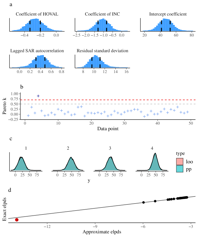
Figure 2: Results of the normal SAR model. 1) Posterior distribution of selected parameters of the lagged SAR model along with posterior median and 50% central interval. 2) PSIS diagnostic plot showing the Pareto-$k$-estimate of each observation. 3) Implied response values of the first four observations computed (a) after model fitting (type = ‘loo’) and (b) as part of the model in the form of posterior-predictive draws for the missing observation (type = ‘pp’). As both distributions are almost identical, the ‘loo’ distribution is hidden behind the ‘pp’ distribution. 4) Comparison of approximate and exact pointwise elpd values. Problematic observations are marked as red dots.

With the correctness of the approximating procedure established for non-problematic observations, we can now go ahead and correct for the problematic observation in the approximate LOO-CV estimate. Vehtari et al., (2017) recommend to perform exact LOO-CV only for the problematic observations and replace their approximate ELPD contributions with their exact counterparts (see also Paananen et al.,, 2019, for an alternative method). So this time, we do not use exact LOO-CV for validation of the approximation but rather to improve the latter’s accuracy when needed. In the present normal SAR model, only the 4th observation was diagnosed as problematic and so we only need to update the ELPD contribution of this observation. The results of the corrected approximate ($\text{elpd}_{\text{approx}}=$ -188.0) and exact LOO-CV ($\text{elpd}_{\text{exact}}=$ -188.1) are now almost equal for the complete data set as well.

Although we were able to correct for the problematic observation in the approximate LOO-CV estimation, the mere existence of such problematic observations raises doubts about the appropriateness of the normal SAR model for the present data. Accordingly, it is sensible to fit a Student-$t$ SAR model as a potentially better predicting alternative due to its fatter tails. We choose an informative ${\rm Gamma}(4,0.5)$ prior (with mean $8$ and standard deviation $4$) on the degrees of freedom parameter $\nu$ to ensure rather fat tails of the likelihood a-priori. For all other parameters, we continue to use the weakly-informative default priors of brms. In Figure 3 (a), the marginal posterior distributions of the main model parameters are depicted. Comparing the results to those shown in Figure 2 (a), we see that the estimates of both the regression parameters and the SAR autocorrelation are quite similar to the estimates obtained from the normal model.

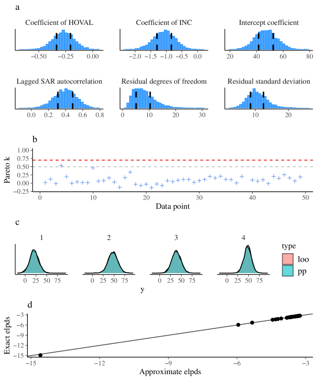
Figure 3: Results of the Student-$t$ SAR model. a) Posterior distribution of selected parameters of the lagged SAR model along with posterior median and 50% central interval. b) PSIS diagnostic plot showing the Pareto-$k$-estimate of each observation. c) Implied response values of the first four observations computed (1) after model fitting (type = ‘loo’) and (2) as part of the model in the form of posterior-predictive draws for the missing observation (type = ‘pp’). As both distributions are almost identical, the ‘loo’ distribution is hidden behind the ‘pp’ distribution. d) Comparison of approximate and exact pointwise elpd values. There were no problematic observations for this model.

In contrast to the normal case, we see in Figure 3 (b) that the 4th observation is no longer recognized as problematic by the Pareto-$k$ diagnostics. It does exceed $0.5$ slightly but does not exceed the more important threshold of $0.7$ above which we would stop trusting the PSIS-LOO-CV approximation. Indeed, comparison between the approximate ($\text{elpd}_{\text{approx}}=$ -187.7) and exact LOO-CV ($\text{elpd}_{\text{exact}}=$ -187.9) based on the complete data demonstrates that they are very similar (up to random error due to the MCMC estimation). The results shown in Figure 3 (c) and (d) have the same interpretation as the analogous plots for the normal case and provide further evidence for both the correctness of our (exact and approximate) LOO-CV methods for non-factorized Student-$t$ models and for the quality of the PSIS-LOO-CV approximation for the present Student-$t$ SAR model.

Lastly, let us compare the PSIS-LOO-CV estimate of the normal SAR model (after correcting for the problematic observation via refit) to the Student-$t$ SAR model. The ELPD difference between the two models is -0.3 (SE = 0.5) in favor of the Student-$t$ model, and thus very small and not substantial for any practical purposes. As shown in Figure 4, the pointwise elpd contributions are also highly similar. The Student-$t$ model fits slightly but noticeably better only for the 4th observation. Other methods clearly identify the 4th observation as problematic as well (e.g., Halleck Vega and Elhorst,, 2015). However, what exactly causes this outlier remains unclear so far as nobody has been able to verify or spatially register the data set despite many attempts.

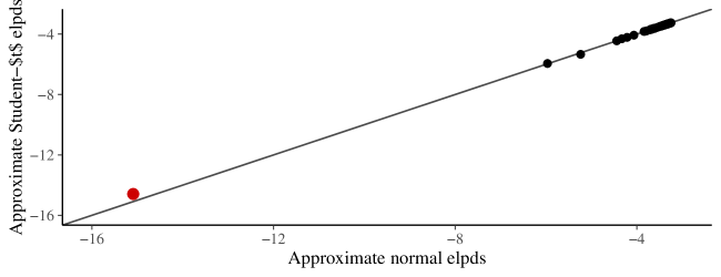
Figure 4: Comparison of approximate pointwise elpd values for the normal SAR model (after refit for the 4th observation) and the Student-$t$ SAR model (without refit). Observations with relevant differences are highlighted in red.

5 Conclusion

In this paper we derived how to perform and validate exact and approximate leave-one-out cross-validation (LOO-CV) for non-factorized multivariate normal and Student-$t$ models and we demonstrated the practical applicability of our method in a case study using spatial autoregressive models. The proposed LOO-CV approximation makes efficient and robust model fit evaluation and comparison feasible for many models that are widely used in temporal and spatial statistics. Importantly, our method does not only apply to non-factorizable models for which a factorized likelihood is unavailable. It is also useful when factorization is possible in principle but could result in a unstable LOO predictive density, either for numerical reasons or due to the use of finite estimation procedures like Markov-Chain Monte Carlo. In such cases, marginalizing over observation-specific latent variables and using a non-factorized formulation can lead to more robust estimates.

6 Acknowledgements

We thank Daniel Simpson for useful discussion and the Academy of Finland (grants 298742, 313122) as well as the Technology Industries of Finland Centennial Foundation (grant 70007503; Artificial Intelligence for Research and Development) for partial support of this work.

Appendix

Proof of Proposition 1. In their Lemma 1, Sundararajan and Keerthi, (2001) prove for any finite subset $z$ of a zero-mean Gaussian process with covariance matrix $\Sigma$ that the LOO predictive mean and standard deviation can be computed as

$$\tilde{\mu}_{i}=z_{i}-\frac{g_{i}}{\bar{\sigma}_{ii}},$$ (29)

$$\tilde{\sigma}_{i}=\frac{1}{\bar{\sigma}_{ii}},$$ (30)

where $g_{i}=\left[\Sigma^{-1}z\right]_{i}$ and $\bar{\sigma}_{ii}=\left[\Sigma^{-1}\right]_{ii}$. Their proof does not make use of any specific form of $\Sigma$ and thus directly applies to all zero-mean multivariate normal distributions. If $y$ is multivariate normal with mean $\mu$ then $(y-\mu)$ is multivariate normal with mean $0$ and unchanged covariance matrix. Thus, we can replace $z$ with $(y-\mu)$ in the above equations. By the same argument we see that, if $(y_{i}-\mu_{i})$ has LOO mean $(y_{i}-\mu_{i})-\frac{g_{i}}{\bar{\sigma}_{ii}}$, then $y$ has LOO mean $y_{i}-\frac{g_{i}}{\bar{\sigma}_{ii}}$ which completes the proof. $\Box$

Proof of Proposition 2. Using the parameterization $K:={\rm Cov}(y)=\frac{\nu}{\nu-2}\Sigma$ and requiring $\nu>2$, Shah et al., (2014) proof in their Lemma 3 that, if $y=(y_{1},y_{2})$ is multivariate Student-$t$ of dimension $N=N_{1}+N_{2}$, then $y_{2}$ given $y_{1}$ is multivariate Student-$t$ of dimension $N_{2}$. Moreover, they provide equations for the parameters of the conditional Student-$t$ distribution. When we parameterize for $\Sigma$ instead of $K$ and allow for $\nu>0$, we can repeat their proof analogously which yields the following parameters of the conditional Student-$t$ distribution of $y_{2}$ given $y_{1}$:

$$\tilde{\nu}_{2}=\nu+N_{1},$$ (31)

$$\tilde{\mu}_{2}=\mu_{2}+\Sigma_{2,1}\Sigma^{-1}_{1}(y_{1}-\mu_{1}),$$ (32)

$$\tilde{\sigma}_{2}=\frac{\nu+\beta_{1}}{\nu+N_{1}}\left(\Sigma_{22}+\Sigma_{2,1}\Sigma^{-1}_{1}\Sigma_{1,2}\right),$$ (33)

with

$$\beta_{1}=(y_{1}-\mu_{1})^{\rm T}\Sigma^{-1}_{1}(y_{1}-\mu_{1}).$$ (34)

where we use the subscripts $1$ and $2$ to refer to the $1$st and $2$nd subset of $y$, respectively. Setting $y_{1}=y_{-i}$, $y_{2}=y_{i}$ for $i=1,\ldots,N$ and noting that $N_{1}=N_{-i}=N-1$ completes the proof. $\Box$

Proof of Proposition 3. The correctness of Equations (16) and (17) follows directly from Equations (8), and (9). To show (18), we perform a rank-one update of $\Sigma^{-1}$ as per Theorem 2.1 of Juárez-Ruiz et al., (2016) based on the Sherman-Morrison formula (Bartlett,, 1951; Sherman and Morrison,, 1950). In general, if we exclude row $p$ and column $q$ from $\Sigma$, the inverse $\Sigma^{-1}_{-p,-q}$ of $\Sigma_{-p,-q}$ exists if $\sigma_{pq}\neq 0$ and $\bar{\sigma}_{pq}\neq 0$. The elements $m_{jk}$ ($j,k=1,\ldots,N$, $j\neq p$, $k\neq q$) of $\Sigma^{-1}_{-p,-q}$ are then given by

$$m_{jk}=\bar{\sigma}_{jk}-\frac{\bar{\sigma}_{jp}\bar{\sigma}_{qk}}{\bar{\sigma}_{pq}}.$$ (35)

where $\bar{\sigma}_{jk}$ is the $(j,k)$th element of $\Sigma^{-1}$. We now set $p=q=i$ and note that $\sigma_{ii}>0$ and $\bar{\sigma}_{ii}>0$ since $\Sigma$ is a covariance matrix, which leads to

$$m_{jk}=\bar{\sigma}_{jk}-\frac{\bar{\sigma}_{ji}\bar{\sigma}_{ik}}{\bar{\sigma}_{ii}}.$$ (36)

for each $i=1,\ldots,N$. Switching to matrix notation completes the proof. $\Box$

References

- Ando and Tsay, (2010) Ando, T. and Tsay, R. (2010). Predictive likelihood for Bayesian model selection and averaging. International Journal of Forecasting, 26(4):744–763.
- Anselin, (1988) Anselin, L. (1988). Spatial econometrics: methods and models. Dordrecht: Kluwer Academic.
- Bartlett, (1951) Bartlett, M. S. (1951). An inverse matrix adjustment arising in discriminant analysis. The Annals of Mathematical Statistics, 22(1):107–111.
- Bivand and Piras, (2015) Bivand, R. and Piras, G. (2015). Comparing implementations of estimation methods for spatial econometrics. Journal of Statistical Software, 63(18):1–36.
- Bürkner, (2017) Bürkner, P.-C. (2017). brms: An R package for Bayesian multilevel models using Stan. Journal of Statistical Software, 80(1):1–28.
- Bürkner, (2018) Bürkner, P.-C. (2018). Advanced Bayesian multilevel modeling with the R package brms. The R Journal, pages 395–411.
- Carpenter et al., (2017) Carpenter, B., Gelman, A., Hoffman, M., Lee, D., Goodrich, B., Betancourt, M., Brubaker, M. A., Guo, J., Li, P., and Ridell, A. (2017). Stan: A probabilistic programming language. Journal of Statistical Software.
- Cressie, (1992) Cressie, N. (1992). Statistics for spatial data. Terra Nova, 4(5):613–617.
- Fernández and Steel, (1999) Fernández, C. and Steel, M. F. (1999). Multivariate student-t regression models: Pitfalls and inference. Biometrika, 86(1):153–167.
- Geisser and Eddy, (1979) Geisser, S. and Eddy, W. F. (1979). A predictive approach to model selection. Journal of the American Statistical Association, 74(365):153–160.
- Gelfand et al., (1992) Gelfand, A., Dey, D., and Chang, H. (1992). Model determination using predictive distributions with implementation via sampling-based methods. Bayesian Statistics, 4:147–167.
- Gelfand and Vounatsou, (2003) Gelfand, A. E. and Vounatsou, P. (2003). Proper multivariate conditional autoregressive models for spatial data analysis. Biostatistics, 4(1):11–15.
- Goulard et al., (2017) Goulard, M., Laurent, T., and Thomas-Agnan, C. (2017). About predictions in spatial autoregressive models: Optimal and almost optimal strategies. Spatial Economic Analysis, 12(2-3):304–325.
- Haining and Haining, (2003) Haining, R. P. and Haining, R. (2003). Spatial data analysis: theory and practice. Cambridge university press.
- Halleck Vega and Elhorst, (2015) Halleck Vega, S. and Elhorst, J. P. (2015). The slx model. Journal of Regional Science, 55(3):339–363.
- Hoeting et al., (1999) Hoeting, J. A., Madigan, D., Raftery, A. E., and Volinsky, C. T. (1999). Bayesian model averaging: a tutorial. Statist. Sci., 14(4):382–417.
- Juárez-Ruiz et al., (2016) Juárez-Ruiz, E., Cortés-Maldonado, R., and Pérez-Rodríguez, F. (2016). Relationship between the inverses of a matrix and a submatrix. Computación y Sistemas, 20(2):251–262.
- LeSage and Pace, (2009) LeSage, J. P. and Pace, R. K. (2009). Introduction to Spatial Econometrics. CRC Press.
- O’Hagan, (1979) O’Hagan, A. (1979). On outlier rejection phenomena in Bayes inference. Journal of the Royal Statistical Society: Series B (Methodological), 41(3):358–367.
- Paananen et al., (2019) Paananen, T., Piironen, J., Bürkner, P.-C., and Vehtari, A. (2019). Pushing the limits of importance sampling through iterative moment matching. arXiv preprint arXiv:1906.08850.
- Piché et al., (2012) Piché, R., Särkkä, S., and Hartikainen, J. (2012). Recursive outlier-robust filtering and smoothing for nonlinear systems using the multivariate student-t distribution. In 2012 IEEE International Workshop on Machine Learning for Signal Processing, pages 1–6. IEEE.
- Rabiner and Juang, (1986) Rabiner, L. and Juang, B. (1986). An introduction to hidden Markov models. ieee assp magazine, 3(1):4–16.
- Rasmussen, (2003) Rasmussen, C. E. (2003). Gaussian processes in machine learning. In Summer School on Machine Learning, pages 63–71. Springer.
- Shah et al., (2014) Shah, A., Wilson, A., and Ghahramani, Z. (2014). Student-t processes as alternatives to Gaussian processes. In Artificial intelligence and statistics, pages 877–885.
- Sherman and Morrison, (1950) Sherman, J. and Morrison, W. J. (1950). Adjustment of an inverse matrix corresponding to a change in one element of a given matrix. The Annals of Mathematical Statistics, 21(1):124–127.
- Sundararajan and Keerthi, (2001) Sundararajan, S. and Keerthi, S. S. (2001). Predictive approaches for choosing hyperparameters in Gaussian processes. Neural Computation, 13(5):1103–1118.
- Tong, (2012) Tong, Y. L. (2012). The multivariate normal distribution. Springer Science & Business Media.
- Vehtari et al., (2018) Vehtari, A., Gabry, J., Yao, Y., and Gelman, A. (2018). loo: Efficient Leave-One-Out Cross-Validation and WAIC for Bayesian Models. R package version 2.0.0.
- Vehtari et al., (2017) Vehtari, A., Gelman, A., and Gabry, J. (2017). Practical Bayesian model evaluation using leave-one-out cross-validation and WAIC. Statistics and Computing, 27(5):1413–1432.
- Vehtari and Ojanen, (2012) Vehtari, A. and Ojanen, J. (2012). A survey of Bayesian predictive methods for model assessment, selection and comparison. Statistics Surveys, 6:142–228.
- Vehtari et al., (2019) Vehtari, A., Simpson, D., Gelman, A., Yao, Y., and Gabry, J. (2019). Pareto smoothed importance sampling. arXiv preprint.
- Welch et al., (1995) Welch, G., Bishop, G., et al. (1995). An introduction to the Kalman filter.
- Zellner, (1976) Zellner, A. (1976). Bayesian and non-Bayesian analysis of the regression model with multivariate Student-t error terms. Journal of the American Statistical Association, 71(354):400–405.
- Zhang and Yeung, (2010) Zhang, Y. and Yeung, D.-Y. (2010). Multi-task learning using generalized t process. In Proceedings of the Thirteenth International Conference on Artificial Intelligence and Statistics, pages 964–971.