Impact of Weak Lensing Mass Calibration on eROSITA Galaxy Cluster Cosmological Studies – a Forecast

Abstract

We forecast the impact of weak lensing (WL) cluster mass calibration on the cosmological constraints from the X-ray selected galaxy cluster counts in the upcoming eROSITA survey. We employ a prototype cosmology pipeline to analyze mock cluster catalogs. Each cluster is sampled from the mass function in a fiducial cosmology and given an eROSITA count rate and redshift, where count rates are modeled using the eROSITA effective area, a typical exposure time, Poisson noise and the scatter and form of the observed X-ray luminosity– and temperature–mass–redshift relations. A subset of clusters have mock shear profiles to mimic either those from DES and HSC or from the future Euclid and LSST surveys. Using a count rate selection, we generate a baseline cluster cosmology catalog that contains 13k clusters over 14,892 deg² of extragalactic sky. Low mass groups are excluded using raised count rate thresholds at low redshift. Forecast parameter uncertainties for $\Omega_{\mathrm{M}}$, $\sigma_{8}$ and $w$ are 0.023 (0.016; 0.014), 0.017 (0.012; 0.010), and 0.085 (0.074; 0.071), respectively, when adopting DES+HSC WL (Euclid; LSST), while marginalizing over the sum of the neutrino masses. A degeneracy between the distance–redshift relation and the parameters of the observable–mass scaling relation limits the impact of the WL calibration on the $w$ constraints, but with BAO measurements from DESI an improved determination of $w$ to 0.043 becomes possible. With Planck CMB priors, $\Omega_{\text{M}}$ ($\sigma_{8}$) can be determined to $0.005$ ($0.007$), and the summed neutrino mass limited to $\sum m_{\nu}<0.241$ eV (at 95%). If systematics on the group mass scale can be controlled, the eROSITA group and cluster sample with 43k objects and LSST WL could constrain $\Omega_{\mathrm{M}}$ and $\sigma_{8}$ to 0.007 and $w$ to 0.050.

1 Introduction

Over the last decade, measuring the number density of galaxy clusters as a function of observable and redshift has proven to be a potent way to determine not only the density and clustering of matter in the Universe, but also to shed light on the yet unknown source of the late time accelerated expansion of the Universe (Koester et al., 2007; Vikhlinin et al., 2009b; Mantz et al., 2010; Rozo et al., 2010; Benson et al., 2013; Mantz et al., 2015; Bocquet et al., 2015; Planck Collaboration et al., 2016b; de Haan et al., 2016; Bocquet et al., 2018). To this end, ever larger samples of galaxy clusters have been selected in X-rays (Vikhlinin et al., 1998; Böhringer et al., 2001; Romer et al., 2001; Clerc et al., 2014; Klein et al., 2019), at millimeter wavelengths (Hasselfield et al., 2013; Bleem et al., 2015; Planck Collaboration et al., 2016c), and in the optical (Koester et al., 2007; Rykoff et al., 2016). Extracting accurate cosmological constraints from these samples depends critically on the ability to determine the mapping between the observable in which the samples have been selected, and the halo mass over the relevant range of redshifts. This aspect is commonly referred to as mass calibration.

Two main methods have been developed for this purpose. The first– weak lensing (hereafter WL)– the coherent distortion of the shapes of galaxies behind galaxy clusters by the cluster gravitational potential has proven to be the method of choice to calibrate masses (e.g., Bardeau et al., 2007; Okabe et al., 2010; Hoekstra et al., 2012; Applegate et al., 2014; Israel et al., 2014; Melchior et al., 2015; Okabe & Smith, 2016; Melchior et al., 2017; Schrabback et al., 2018a; Dietrich et al., 2019). Alternatively, the dynamics of the cluster galaxies themselves has been used within recent cluster surveys to calibrate the cluster halo masses (Sifón et al., 2013; Bocquet et al., 2015; Capasso et al., 2019; Zhang et al., 2017). On individual clusters, these methods characteristically provide a low signal to noise mass constraint with low bias that, importantly, can be reliably characterized using numerical structure formation simulations. For example, the scaling between the mass observed through WL (hereafter the WL mass) and the halo mass can be calibrated to robustly characterize the biases and scatter (e.g., Becker & Kravtsov, 2011). With modern hydrodynamical simulations it is now possible to include baryon physics in this calibration (Lee et al., 2018). Similarly, the biases and scatter in dynamical mass estimators can be characterized using numerical simulations (e.g., Evrard et al., 2008; Mamon et al., 2013) in a manner that includes the impact of the (red) galaxy sample selection (Saro et al., 2013).

A third method– hydrostatic masses using X-ray observations– has played an important role in the development of our understanding of galaxy clusters, but through simulation studies and comparison with WL masses, these hydrostatic masses have been shown to be biased at the $\sim 20$% level or more (see, e.g., Nagai et al., 2007; Rasia et al., 2012; von der Linden et al., 2014; Hoekstra et al., 2015; Shi et al., 2015; Planck Collaboration et al., 2016b, 2018), although the scale of the bias remains a topic of ongoing research (Smith et al., 2016; Gupta et al., 2017). This hydrostatic mass bias together with the availability of shear catalogs from deep, multiband surveys and the increasingly large wide field spectroscopic datasets, have created a situation where the X-ray hydrostatic masses no longer offer clear benefits within the context of large scale cluster cosmological studies.

The low signal to noise of individual cluster WL mass measurements is compensated to some degree by the larger number of galaxy clusters that can be studied. This stems from the fact that, in addition to the cluster observables of redshift and position, cluster weak lensing mass calibration requires the same data as cosmic shear experiments. The advent of deep, large area photometric imaging surveys with a well controlled point spread function correction for accurate shape measurements and high quality photometric redshifts now enables the WL study of large samples of galaxy clusters (Melchior et al., 2015; Murata et al., 2018; Miyatake et al., 2018; McClintock et al., 2019; Stern et al., 2019).

It is in this context that we investigate the impact of WL mass calibration on the cluster cosmology results from the X-ray selected sample that will be extracted from the all sky X-ray survey undertaken with the forthcoming eROSITA telescope (Predehl et al., 2010; Merloni et al., 2012) on board the Russian "Spectrum-Roentgen-Gamma" satellite. Previous analyses adopting a Fisher matrix approach have explored the constraining power of the eROSITA cluster sample on non Gaussianities (Pillepich et al., 2012) and the dark energy equation of state parameter (Pillepich et al., 2018), further underscoring the promise of cluster number counts as a cosmological probe (e.g., Haiman et al., 2001).

In this work, we create a mock cluster catalog with characteristics of the expected eROSITA catalog, and we use a prototype of the eROSITA cluster cosmology analysis code to perform the number counts experiment. We consider the improvement in constraining power when the eROSITA X-ray cluster catalog is calibrated with realistic WL lensing shear profiles from the ongoing Dark Energy Survey (DES, Dark Energy Survey Collaboration et al., 2016) and Hyper-Suprime-Cam Survey (HSC, Miyazaki et al., 2018), and the forthcoming Euclid (Laureijs et al., 2011) and Large Synoptic Survey Telescope (LSST, Ivezic et al., 2008) surveys. We explore parameter sensitivities and probe for limiting degeneracies in the analysis. Finally, we explore the synergies of combining the eROSITA cluster counts cosmological constraints with those from existing CMB temperature anisotropy measurements (Planck Collaboration et al., 2016a) and with those from the future DESI BAO measurements (Levi et al., 2013).

The paper is organized as follows: in Section 2 we discuss how we create the mock data. In Section 3 we discuss the modeling used to determine the cosmological parameters, and we present and validate a prototype of the eROSITA cosmological analysis pipeline. In Section 4, we present the results of the impact of WL mass calibration on our knowledge of the cosmological parameters and the observable mass relation. Various aspects of these results together with the parameter sensitivities and important degeneracies are then discussed in Section 5. We conclude this work by summarizing the main results in Section 6.

2 Experimental setup

To constrain the impact of direct mass calibration through WL tangential shear measurements on eROSITA cluster cosmology, we create an eROSITA mock cluster catalog. The actual eROSITA cluster candidate catalog will be extracted from the eROSITA X-ray sky survey using specially designed detection and characterization tools (Brunner et al., 2018).

Each candidate source will be assigned a detection significance, an extent significance, an X-ray count rate and uncertainty, and other more physical parameters such as the flux within various observing bands (Merloni et al., 2012). For a subset of this sample, precise X-ray temperatures and rough X-ray redshifts will also be available (Borm et al., 2014; Hofmann et al., 2017).

This X-ray cluster candidate catalog will then be studied in the optical to identify one or more optical counterparts (assigning a probability to each) and to estimate a photometric redshift. A special purpose Multi-Component-Matched-Filter (MCMF) optical followup tool (Klein et al., 2018) has been designed for eROSITA cluster analysis and has been tested on available X-ray and SZE catalogs. It has been shown in RASS+DES analyses that one can reliably obtain both cluster and group redshifts over the relevant ranges of redshift (Klein et al., 2019), and thus for the analysis undertaken here we assume redshifts are available for all the eROSITA clusters.

The MCMF tool also allows one to quantify the probability of chance superposition between X-ray cluster candidates and optical counterparts, using the statistics of optical systems along random lines of sight together with estimates of the initial contamination in the X-ray cluster candidate catalog. Synthetic sky simulations by Clerc et al. (2018) have shown that the initial X-ray cluster candidate list selected on both detection and extent significance will be contaminated at the 10% level, consistent with experience in X-ray selection from archival ROSAT PSPC data that have a similar angular resolution to eROSITA (Vikhlinin et al., 1998). After processing with MCMF the resulting eROSITA X-ray cluster catalog is expected to have contamination at the sub-percent level. Therefore, we do not include contamination in the mock catalogs produced for this study.

For the WL mass calibration we will be using shear and photometric redshift catalogs from wide field, deep extragalactic surveys, including DES and HSC in the near term and Euclid and LSST on the longer term. The label “Euclid” refers to the nominal requirements for Euclid (Laureijs et al., 2011), although these requirements will realistically be met when combining Euclid with LSST, where the LSST data would be used for the photometric redshifts. We also explore the impact of LSST WL alone, where we adopt the requirements described in the following references(LSST DESC, 2012; LSST DESC et al., 2018). There is also the promise of CMB lensing as another method of mass calibration that is expected to be especially helpful for the highest redshift end of our cluster sample, but in our current analysis we do not model the impact of CMB lensing.

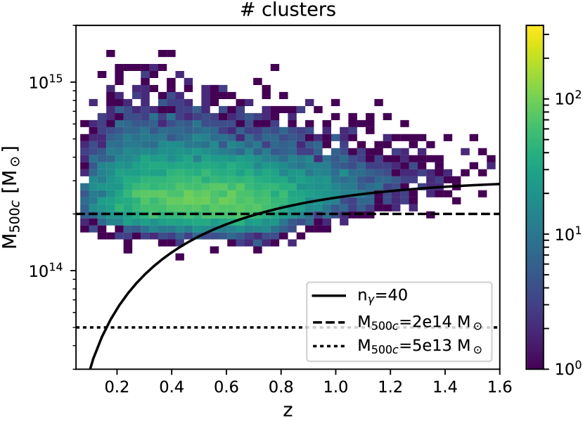
Figure 1: Distribution in halo mass $M_{\text{500c}}$ and cluster redshift $z$ of the mock, X-ray selected cluster catalogs used in this analysis. Left: Above redshift $\sim 0.7$, the 13k cluster baseline sample is selected using the fiducial count rate cut $\eta=2.5\times 10^{-2}$ cts s^-1 that corresponds approximately to 40 photons at the median exposure time and a signal to noise $\xi_{\mathrm{det}}>7$. Below that redshift the observable cut is pushed upward to mimic a mass exclusion at $M_{\text{500c}}\sim 2\times 10^{14}\text{M}_{\sun}$. Due to intrinsic and observational scatter between halo mass and the observable count rate, the cuts in observable used to create these samples appear smoothed in halo mass-redshift space. Right: The 43k sample that includes groups is selected similarly but the count rate cut is adjusted to mimic a mass exclusion at $M_{\text{500c}}\sim 5\times 10^{13}\text{M}_{\sun}$.

Our strategy in the analysis that follows is to adopt direct, cosmology independent cluster observables, including the cluster (1) X-ray detection significance or count rate, (2) photometric redshift, (3) WL tangential shear profile and (4) shear source redshift distributions for use in the cosmological analysis of the cluster sample. A benefit of using the count rate rather than the physical flux is that uncertainties in effective area and the temperature dependence of the conversion from count rate to physical flux do not contribute to cosmological uncertainties.

Empirically mapping these observables to mass as a function of redshift and testing consistency of observed and theoretical cluster distributions as a function of cosmological parameters is described in Section 3. Below, in Section 2.1, we describe how the mock cluster catalog is generated and how the X-ray and optical cluster properties are assigned. In Section 2.2 we describe how we model the shear profiles that are produced for an appropriate subset of the mock eROSITA cluster sample. We discuss briefly our choice of fiducial cosmology and input X-ray scaling relations in Section 2.3.

2.1 Creating the mock cluster catalog

To create the X-ray catalog, we perform the following calculations.

1. For our choice of input cosmology (see Table 1 and Section 2.3), we compute the number of expected clusters as a function of halo mass $M_{500\text{c}}$ and redshift $z$ using the halo mass function (Tinker et al., 2008). We then draw a Poisson realization of the number of expected clusters, obtaining a mass selected cluster sample with $M_{500\text{c}}>1.3\times 10^{13}\text{M}_{\sun}$ and $0.05<z<1.8$. For this calculation we assume a survey solid angle of $\text{Area}_{\text{DE}}=0.361\times 4\pi$, corresponding to regions of the western galactic hemisphere with a galactic hydrogen column $N_{\text{H}}<10^{21}$ cm^-2 (Kalberla et al., 2005).

   This corresponds approximately to a galactic latitude cut of $|b|>20$ deg. We adopt the cluster true redshift as the photometric redshift, because the MCMF optical followup tool has been demonstrated to achieve photometric redshift uncertainties with the DES dataset with an accuracy of $\sigma_{z}/(z+1)\loa 0.01$ (Klein et al., 2018; Klein et al., 2019) out to redshifts $z\sim 1.1$. Photometric redshift uncertainties at this level are small enough to play no role in the cosmological analysis of the eROSITA cluster counts.

2. We use the scaling between X-ray luminosity $L_{[0.5-2]\text{keV}}$ ($L_{X}$ hereafter) in the rest frame $0.5-2$ keV band and halo mass

   $$\frac{L_{X}}{L_{0}}=e^{\ln A_{\text{L}}}\left(\frac{M_{500\text{c}}}{M_{0}}\right)^{B_{\text{L}}}\left(\frac{E(z)}{E_{0}}\right)^{2}\left(\frac{1+z}{1+z_{0}}\right)^{\gamma_{\text{L}}}e^{\Delta_{\text{L}}},$$ (1)

   that was extracted from a large sample of SPT selected clusters with pointed XMM-Newton observations (Bulbul et al., 2019). In this relation $E(z)=H(z)/H_{0}$ encodes the expansion history of the universe and is used to calculate the impact of changes in the critical density of the Universe ($\rho_{\mathrm{crit}}\propto E^{2}(z)$), $\ln A_{\text{L}}$, $B_{\text{L}}$ and $\gamma_{\text{L}}$ are the amplitude, the mass trend and the non-self-similar redshift trend parameters of the luminosity–mass scaling relation, and $\Delta_{\text{L}}\sim\mathcal{N}(0,\sigma^{2}_{\text{L}})$ is a random number drawn from a Gaussian with standard deviation $\sigma_{\text{L}}$, which models the log-normal intrinsic scatter of the relation.

   The Bulbul et al. (2019) X-ray scaling relations are derived from the Sunyaev-Zel’dovich effect (SZE) selected cluster sample from the SPT-SZ 2500 deg² survey (Carlstrom et al., 2011; Bleem et al., 2015) that have available XMM-Newton observations. This is a sample of 59 clusters with $0.2\leq z\leq 1.5$ and masses $M_{500\text{c}}>3\times 10^{14}\text{M}_{\sun}$. These halo masses have been calibrated separately in a cosmological analysis (de Haan et al., 2016) and exhibit a characteristic uncertainty of $\sim$20% (statistical) and $\sim 15$% (systematic). The scaling relation parameter uncertainties from Bulbul et al. (2019) include both statistical and systematic uncertainties.

   We also utilize the temperature mass relation

   $$\frac{T}{T_{0}}=e^{\ln A_{\text{T}}}\left(\frac{M_{500\text{c}}}{M_{0}}\right)^{B_{\text{T}}}\left(\frac{E(z)}{E_{0}}\right)^{\frac{2}{3}}\left(\frac{1+z}{1+z_{0}}\right)^{\gamma_{\text{T}}}e^{\Delta_{\text{T}}},$$ (2)

   from the same analysis (Bulbul et al., 2019), where the parameters $(\ln A_{\text{T}},B_{\text{T}},\gamma_{\text{T}})$ have the same meaning as in the luminosity scaling relation, with $\Delta_{\text{T}}\sim\mathcal{N}(0,\sigma^{2}_{\text{T}})$ for the scatter $\sigma_{\text{T}}$. The only difference is the scaling with the critical density, derived from self similar collapse theory.

   Following these relations, we attribute to each cluster an X-ray luminosity $L_{\text{X}}$ and a temperature $T$, randomly applying the respective intrinsic log normal scatter and assuming that the two scatters are uncorrelated.

3. Given the cluster rest frame 0.5-2 keV luminosity $L_{\text{X}}$ and its redshift $z$, we compute the rest frame 0.5-2 keV flux

   $$f_{\text{X}}=\frac{L_{X}}{4\pi d_{\mathrm{L}}^{2}(z)},$$ (3)

   where $d_{\mathrm{L}}(z)$ is the luminosity distance.

4. For each cluster we calculate the X-ray spectrum assuming an APEC plasma emission model (Smith et al., 2001) with temperature $T$ and metallicity $Z=0.3$ Z_☉. This spectrum is normalized to the cluster rest frame 0.5-2 keV flux.

5. We compute the eROSITA count rate $\eta$ for each cluster by shifting the spectrum to the observed frame and by averaging it with the eROSITA Ancillary Response Function (hereafter ARF) in the observed frame 0.5-2 keV band. For simplicity, we do not follow the variation in neutral hydrogen column across the eROSITA-DE field. In fact, we ignore the impact of Galactic absorption altogether in our count rate calculation, which for the median neutral hydrogen column density in our footprint, $N_{\text{H}}=3\times 10^{20}$ cm^-2 would lead on average to 5% lower rates.

6. To model the measurement uncertainty on the rate, we draw a Poisson realization of the expected rate $\hat{\eta}=\eta\pm\sqrt{\eta/t_{\text{exp}}}$, where $t_{\text{exp}}=1600$ s is the expected median exposure time of the 4 year eROSITA survey (Pillepich et al., 2012). With this we account for the Poisson noise in the rate measurement. The count rate uncertainty for each cluster will be included in the real eROSITA cluster catalogs.

7. Finally, we select our baseline cluster sample using the count rate $\eta>2.5\times 10^{-2}$ ct s^-1 (corresponding for our median exposure to $\hat{n}_{\gamma}>40$). For reference, given the background expectations, survey PSF and clusters modeled as $\beta$ models with core radii that are 20% of the virial radius $r_{500}$, this selection threshold corresponds approximately to a cut in detection significance of $\xi_{\text{det}}>7$, irrespective of the cluster redshift. Simple mock observations (see discussion in Appendix A) indicate that at this threshold and above the extent likelihood for the eROSITA sample is $\xi_{\text{ext}}>2.5$, enabling an initial eROSITA cluster candidate list after X-ray selection (but prior to optical followup) that is contaminated at the $\sim$10% level. At low redshift ($z<0.7$), we raise the detection threshold above the nominal level in such a way as to exclude most clusters with masses $M_{\text{500c}}\lessapprox 2\times 10^{14}\text{M}_{\sun}$ at each redshift. We create a second sample to examine the impact of lower mass clusters and groups (see Section 4.6) by adjusting the low redshift count rate cut so that systems with masses $M_{\text{500c}}\lessapprox 5\times 10^{13}\text{M}_{\sun}$ are excluded at each redshift. We discuss the X-ray selection in more detail in Appendix A. The reasons for excluding lower mass systems are discussed below (cf. Section 4.6).

The procedure described above provides us with a baseline cosmology catalog of $\sim 13$k clusters. Their distribution in halo mass and redshift is shown in the left panel of Fig. 1. They span a redshift range $z\in(0.05,1.6)$. The total number of clusters and their redshift range are mainly impacted by the choice of the input cosmology, the observed luminosity mass relation, and the choice of cut in eROSITA count rate for selection. The sample has a median redshift $\bar{z}=0.51$ and median halo mass of $\bar{M}_{500\text{c}}=2.5\times 10^{14}\text{M}_{\sun}$. This sample extends to high redshift with 3% of the sample, corresponding to 420 clusters, at $z>1$.

The sample of 43k objects with the count rate cut that only excludes lower mass systems with $M_{\text{500c}}\leq 5\times 10^{13}\text{M}_{\sun}$ is shown in Fig. 1 (right). The bulk of the additional low mass systems in this sample appear at redshifts $z\leq 0.7$. As with the overall number of clusters, the median mass and redshift depend on the observable cut used to exclude low mass objects, with these being $\bar{z}=0.30$, and $\bar{M}_{500\text{c}}=1.4\times 10^{14}\text{M}_{\sun}$. We discuss the implications of lowering the mass limit in Section 4.6.

The number of objects in this $\xi_{\mathrm{det}}>7$ group dominated sample is in good agreement with the numbers presented in previous discussions of the eROSITA cluster sample (Merloni et al., 2012; Pillepich et al., 2012, 2018). Importantly, there are significantly more eROSITA clusters that can be detected if one reduces the detection threshold below $\sim 7\sigma$. But at that level there will be little extent information for each X-ray source, and so the candidate sample will be highly contaminated by AGN. Interestingly, Klein et al. (2018) have demonstrated that for the RASS faint source catalog where the survey PSF was so poor that little extent information is available, it is possible to filter out the non-cluster sources to produce low contamination cluster catalogs. The price for this filtering is that one introduces incompleteness for those systems that contain few galaxies (i.e., low mass clusters and groups at each redshift; see Klein et al., 2019).

2.2 Forecasting the WL signal

We adopt the cosmology independent tangential reduced shear profile $\hat{g}_{\text{t}}(\theta_{i})$ in radial bins $\theta_{i}$ around the cluster as the observable for cluster WL mass calibration. A crucial complementary observable is the redshift distribution of the source galaxies $N(z_{\text{s}},z_{\text{cl}})$ behind the galaxy cluster, where $z_{\text{s}}$ is the source redshift, and $z_{\text{cl}}$ the cluster redshift. Assuming that the galaxy cluster mass profile is consistent with a Navarro-Frenk-White model (Navarro et al., 1996, hereafter NFW), these two observables can be combined into a measurement of the halo mass.

Although, in theory, WL mass calibration provides a direct mass measurement, in practice we refer to the mass resulting from an NFW fit to the shear profile as the WL mass $M_{\text{WL}}$. Following Becker & Kravtsov (2011), the WL mass is related to the halo mass by

$$M_{\text{WL}}=b_{\text{WL}}M_{\text{200c}}e^{\Delta_{\text{WL}}},$$ (4)

with $\Delta_{\text{WL}}\sim\mathcal{N}(0,\sigma_{\text{WL}}^{2})$, where $\sigma_{\text{WL}}$ is the intrinsic log- normal scatter between WL mass and halo mass, induced by the morphological deviation of observed galaxy cluster mass profiles from the NFW profile, and $b_{\text{WL}}$ is the WL mass bias describing the characteristic bias in the WL mass compared to the halo mass. This bias encodes several theoretical and observational systematics, as discussed below in Section 3.4.2.

Given that DES, HSC, Euclid and LSST will not overlap completely with the German eROSITA sky, only a fraction $f_{\text{WL}}$ of the galaxy clusters of our X-ray mock catalog will have WL information available. Comparing the survey footprints, we estimate $f_{\text{WL}}=0.3$ for DES, $f_{\text{WL}}=0.05$ for HSC, $f_{\text{WL}}=0.5$ for Euclid, and $f_{\text{WL}}=0.62$ for LSST. For the LSST case we also assume that the northern celestial hemisphere portion of the German eROSITA sky with $0^{\circ}<\delta<30^{\circ}$ will be observed. For this northern extension of LSST, we adopt $f_{\text{WL}}=0.2$ and treat it as if it has the equivalent of DES depth. Therefore, we assign a WL mass only to a corresponding fraction of the eROSITA clusters in our mock catalogs, by drawing from equation (4).

Besides the WL mass and the cluster redshift, the background source distribution of the survey $N(z_{\text{s}})$ in redshift and the background source density $n_{\epsilon}$ are necessary to predict the WL signal. For DES, we project $n_{\epsilon}=10\,\text{arcmin}^{-2}$ and utilize the redshift distribution presented in Stern et al. (2019), whose median redshift is $z_{\text{s,m}}=0.74$. These parameters are derived from the Science Verification Data and their extrapolation to Y5 data will depend on the details of the future calibration (Gruen, priv. comm.). For HSC we assume $n_{\epsilon}=21\,\text{arcmin}^{-2}$, and for the redshift distribution of HSC sources we adapt the parametrization by Smail et al. (1994) with a median redshift $z_{\text{s,m}}=1.1$. For Euclid, we use $n_{\epsilon}=30\,\text{arcmin}^{-2}$ (Laureijs et al., 2011). For the source redshift distribution we assume the parametric form proposed by Smail et al. (1994) and utilized by Giannantonio et al. (2012), adopting a median redshift of $z_{\text{s,m}}=0.9$ (Laureijs et al., 2011). For LSST we assume $n_{\epsilon}=40\,\text{arcmin}^{-2}$ and parametrise the source redshift distribution as $p(z_{\text{s}})=1./(2z_{0})(z_{\text{s}}/z_{0})^{2}\exp(-z_{\text{s}}/z_{0})$ with median redshift $z_{\text{m,s}}=2.67z_{0}=0.8$.

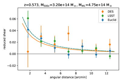
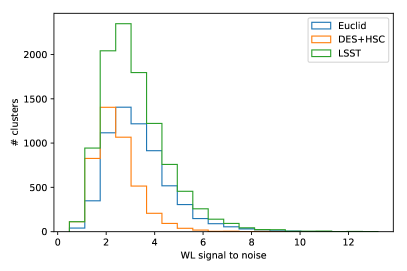
Figure 2: Left: Example of a shear profile in DES (orange), Euclid (blue) and LSST (green) data quality for a cluster. We show both the measured shear profile (dots with error bars) and the prediction (line). For all data quality cases, the measurement uncertainty is larger than the actual signal. Right: Distribution of WL signal to noise for DES+HSC (orange), Euclid (blue) and LSST (green), computed for each single cluster from the measured shear profile and the covariance matrix. While Euclid and LSST provide both more objects and higher signal to noise, objects with a clear WL mass measurement (e.g., S/N$>5$) are rare for all datasets.

The actual redshift distribution behind a galaxy cluster is assumed to be the survey redshift distribution with the cut $N(z_{\text{s}}<z_{\text{cl}}+0.1)=0$, where $z_{\text{cl}}$ is the cluster redshift. This cut is helpful in reducing the contamination of the background source galaxies by cluster galaxies (that are not distorted by the cluster potential). This cut also leads to a reduction of the source density $n_{\epsilon}(z_{\text{s}}>z_{\text{cl}}+0.1)$ used to infer the observational noise on the cluster shear signal.

Given a redshift distribution, the mean reduced shear signal can be estimated, following Seitz & Schneider (1997), as

$$g_{\text{t}}(\theta_{i})=\frac{\gamma(\theta_{i})}{1-\kappa(\theta_{i})}\left(1+\kappa(\theta_{i})\frac{\langle\beta^{2}\rangle}{\langle\beta\rangle^{2}}\right),$$ (5)

where $\gamma(\theta_{i})$ and $\kappa(\theta_{i})$ are the shear and the convergence of an NFW mass profile, $\theta_{i}$ the angular bins corresponding to radii between $0.25$ and $5.0$ Mpc at the cluster redshift in our fiducial cosmology. This has the effect that low redshift clusters will have larger angular bins than high redshift clusters in to probe the similar physical scales. Also note that the inner radius, which we probe ($0.25$ Mpc), is smaller than in some previous studies ($0.75$ Mpc in Applegate et al., 2014; Stern et al., 2019; Dietrich et al., 2019). While this will require a more precise treatment of systematic effects such a cluster member contamination, miscentering and the impact of intra-cluster light on the shape and redshift measurements, theoretical predictions for the resulting WL mass bias and WL mass scatter associated with these smaller inner radii have already been presented (Lee et al., 2018). Furthermore, Gruen et al. (2018) investigated the impact of intra-cluster light on the photometric redshift measurement of background galaxies. We therefore assume that ongoing and future studies will demonstrate the possibility of exploiting shear information at smaller cluster radii, thereby increasing the amount of extracted mass information.

Following Bartelmann (1996), the shear and the convergence can be computed analytically for any halo, given the mass, the concentration, and the source galaxy redshift distribution $N(z_{\text{s}},z_{\text{cl}})$. Throughout this work, the concentration of any cluster will be derived from its halo mass, following the relation presented by Duffy et al. (2008). The scatter in concentration at fixed halo mass is a contributor to the bias $b_{\text{WL}}$ and scatter $\sigma_{\text{WL}}$ in the WL mass to halo mass relation (equation 4). The lensing efficiency $\beta=d_{\mathrm{A}}(z_{\text{cl}},z_{\text{s}})/d_{\mathrm{A}}(z_{\text{s}})$ is the ratio between the angular diameter distance $d_{\mathrm{A}}(z_{\text{cl}},z_{\text{s}})$ from the cluster to the source, and the angular diameter distance $d_{\mathrm{A}}(z_{\text{s}})$ from the observer to the source. In equation (5) the symbol $\langle\cdot\rangle$ denotes averaging over the source redshift distribution $N(z_{\text{s}},z_{\text{cl}})$.

The covariance of the measurement uncertainty on the reduced shear is

$$\mathsf{\mathbf{C}}_{i,j}=\text{Cov}[g_{\text{t}}(\theta_{i}),g_{\text{t}}(\theta_{j})]=\frac{\sigma^{2}_{\epsilon}}{\Omega_{i}n_{\epsilon}(z_{\text{cl}})}\delta_{i,j}+(\mathsf{\mathbf{C}}_{\text{uLSS}})_{i,j}$$ (6)

where $\delta_{i,j}=1$, if $i=j$, and $\delta_{i,j}=0$ else. The first term accounts for the shape noise in each radial bin, estimated by scaling the intrinsic shape noise of the source galaxies $\sigma_{\epsilon}=0.27$ by the number of source galaxies in each radial bin, taking into account the reduction of source galaxy density $n_{\epsilon}(z_{\text{cl}})=n_{\epsilon}(z_{\text{s}}>z_{\text{cl}}+0.1)$ and the angular area of the $i$-th radial bin $\Omega_{i}$. We also add a contribution coming from uncorrelated large scale structure $(\mathsf{\mathbf{C}}_{\text{uLSS}})_{i,j}$ (Hoekstra, 2003). We draw the measured reduced shear profile $\hat{g}_{\text{t}}$ from the Gaussian multivariate distribution with mean $g_{\text{t}}$ and covariance $\mathsf{\mathbf{C}}$.

For each cluster with WL information, we thus save the source redshift distribution $N(z_{\text{s}},z_{\text{cl}})$, the measured reduced shear profile $\hat{g}_{\text{t}}$, and the covariance $C$. We show an example for a measured reduced shear profile, both in DES, in Euclid and in LSST data quality in the left panel of Fig. 2.

The WL signal around individual galaxy clusters derived from wide and deep photometric surveys is typically low signal to noise. In the right panel of Fig. 2, we explore the distribution of WL signal to noise for the subsamples with DES+HSC WL data, Euclid WL data and LSST WL data. To this end we define the signal to noise as $\text{S}/\text{N}=\sqrt{0.5\,\hat{g}_{\text{t}}^{T}\mathsf{\mathbf{C}}^{-1}g_{\text{t}}}$. While the Euclid and LSST data provide a higher signal to noise on average, it rarely exceeds $\text{S}/\text{N}>5$. Thus, we confirm that WL mass calibration provides a low signal to noise, direct mass measurement for a large subset of our cluster catalog.

Table 1: Input parameters for our analysis. The exact definition of the parameters listed below is given in Section 3.3, Section 3.1 and Section 2.2 for the cosmological parameters, the scaling relation parameters and the WL calibration parameters, respectively.
Comments: a) This value is determined to match $\sigma_{8}=0.768$ by de Haan et al. (2016).  b) We utilize here the value corresponding to the minimal model of a Cosmological Constant causing the accelerated expansion. c) This is the minimal value allowed by flavor neutrino oscillations, as reviewed by Tanabashi et al. (2018).

Cosmological Parameters
$H_{\text{0}}$	73.02	Riess et al. (2016)
$\omega_{\text{b}}$	0.02202	Cooke et al. (2014)
$\Omega_{\text{M}}$	0.306	de Haan et al. (2016)
$A_{\text{S}}$	1.5792e-9	a)
$n_{\text{S}}$	0.9655	Planck Collaboration et al. (2016a)
$w$	-1.00	b)
$\sum m_{\nu}$	0.06 eV	c)
$\Omega_{\text{K}}$	0.
Luminosity–Mass–Redshift Relation
$\ln A_{\text{L}}$	1.52	Bulbul et al. (2019)
$B_{\text{L}}$	1.95
$\gamma_{\text{L}}$	-0.20
$\sigma_{L}$	0.237
Temperature–Mass–Redshift Relation
$\ln A_{\text{T}}$	1.83	Bulbul et al. (2019)
$B_{\text{T}}$	0.849
$\gamma_{\text{T}}$	-0.28
$\sigma_{T}$	0.177
WL Mass Bias and Scatter
$b_{\text{WL}}$	0.94	Dietrich et al. (2019) &
$\sigma_{\text{WL}}$	0.24	Lee et al. (2018)

2.3 Fiducial cosmology and scaling relations

Several steps in the above outlined creation of the mock data are cosmology sensitive. Therefore, the choice of input cosmology will impact the catalog properties. As an input cosmology, we choose the best fitting $\Omega_{\text{M}}$ and $\sigma_{8}$ results from the most recent SPT galaxy cluster cosmology analysis (de Haan et al., 2016). We also assumed that dark energy can be described by a cosmological constant, i.e. that the dark energy equation of state parameter $w=-1$. Furthermore, we adopt the minimal neutrino mass allowed by flavor neutrino oscillation measurements, $\sum m_{\nu}=0.06$ eV (Tanabashi et al., 2018). The parameter values are listed in Table 1.

It is worth noting here that these input values for $\Omega_{\text{M}}$ and $\sigma_{8}$ are somewhat different (at less than 2$\sigma$ significance) from the best fit values derived from the Planck CMB anisotropy measurements (Planck Collaboration et al., 2016a). This choice is intentional, as the masses of SPT clusters derived from a mass function fit with Planck CMB priors have been shown to be systematically high by studies of their WL signal (Dietrich et al., 2019; Stern et al., 2019), their dynamical mass (Capasso et al., 2019) and their baryon content (Chiu et al., 2018). Furthermore, the input X-ray scaling relations by Bulbul et al. (2019), adapted to determine the X-ray properties of our catalog entries, assume an SZE signature–mass–redshift scaling relation consistent with the best fit results from the SPT galaxy cluster cosmology analysis. In summary, the input values for our analysis are chosen from the latest results of the SPT galaxy cluster sample, guaranteeing consistency between the assumed cosmology and the input X-ray scaling relations that we use to construct the mock eROSITA sample. Given that SPT covers a mass range of $M_{500\text{c}}\goa 3\times 10^{14}M_{\sun}$, and a redshift range of $z\in(0.20,1.7)$, adopting SPT results within the eROSITA context implies only a modest extrapolation in mass and redshift.

On the other hand, the minimal neutrino mass is slightly inconsistent with recent results from joint fits to number counts of SPT selected clusters and Planck CMB measurements (de Haan et al., 2016; Bocquet et al., 2018), which detect the neutrino mass at $2$-$3$ sigma. This detection is likely sourced by the slight inconsistency in the $(\Omega_{\text{M}},\sigma_{8}$) plane discussed above. For the sake of this work, we adapt the minimal neutrino mass to predict improvement on the upper limits obtained, if cluster number counts and CMB measurements were in perfect agreement.

3 Cosmology analysis method

In this section we describe the method we have developed for the cosmological analysis of an eROSITA cluster sample in the presence of WL mass calibration information. This method builds upon a method developed and used for the analysis of the SPT SZE selected cluster sample (Bocquet et al., 2015; Dietrich et al., 2019; Stern et al., 2019; Bocquet et al., 2018). We start with a description of the minimal scaling relation to describe the mapping of the selection observable to halo mass as a function of redshift (Section 3.1), present the likelihoods in Section 3.2 and discuss the likelihood sampling tool and our adopted priors in Sections 3.3 and 3.4.

3.1 Cluster selection scaling relation

The cosmological analysis of a galaxy cluster sample requires a model for the relation between the halo mass and the observable. In this work, we take an approach which is conceptually similar to the modeling of the scaling relation used for the SPT galaxy cluster sample first presented and applied to derive cosmological constraints by Vanderlinde et al. (2010) (for further applications, see for instance Benson et al. (2013); Bocquet et al. (2015); de Haan et al. (2016); Bocquet et al. (2018)). We empirically calibrate a scaling relation between the selection observable, i.e. the eROSITA count rate $\eta$, and the halo mass and redshift. As motivated in Appendix B, we adopt the following scaling of the count rate with mass and redshift:

$$\begin{split}\frac{\eta}{\eta_{0}}=&e^{\ln{A_{\text{X}}}}\left(\frac{M_{500\text{c}}}{M_{0}}\right)^{B(z)}\left(\frac{E(z)}{E_{0}}\right)^{2}\left(\frac{d_{\text{L}}(z)}{d_{\text{L},0}}\right)^{-2}\\ &\left(\frac{1+z}{1+z_{0}}\right)^{\gamma_{\text{X}}}e^{\Delta_{\text{X}}},\end{split}$$ (7)

where the amplitude is $A_{\text{X}}$, the redshift dependent mass slope is given by

$$B(z)=B_{\text{X}}+B_{\text{X}}^{\prime}\ln\left(\frac{1+z}{1+z_{0}}\right),$$ (8)

the redshift trend describing departures from self-similar evolution is $\gamma_{\text{X}}$, and the deviation of a particular cluster from the mean scaling relation is described as $\Delta_{\text{X}}\sim\mathcal{N}(0,\sigma_{\text{X}}^{2})$, with scatter $\sigma_{\text{X}}$ (i.e., log-normal scatter in observable at fixed halo mass). As pivot points we choose $M_{0}=2\times 10^{14}\text{ M}_{\sun}$, $z_{0}=0.5$, $E_{0}=1.314$, $d_{\mathrm{L,0}}=2710$ Mpc, and $\eta_{0}=0.06$ cts s^-1.

Empirical calibration of the scaling relation has some major advantages compared to trying to measure accurate physical cluster quantities such as the flux. In doing the latter, the one might suffer biases (e.g. the effect of substructures in the context of eROSITA found by Hofmann et al., 2017) or additional sources of scatter from lack of knowledge about the cluster physical state. Furthermore, any such biases might themselves have trends with mass or redshift. An alternative approach, which has been adopted with success within SPT, is to use mass calibration to empirically determine the values of the scaling relation parameters. In this approach, an unbiased solution is found assuming the correct likelihood is adopted (see Section 3.2) and that the form of the observable mass scaling relation that is adopted has sufficient flexibility to describe the cluster population. One can examine this using goodness of fit tests (see Bocquet et al., 2015; de Haan et al., 2016). There is now considerable evidence in the literature that empirical calibration leads to a more robust cosmological experiment.

In summary, our model for the rate mass scaling assumes that the rate is a power law in mass and redshift with log-normal intrinsic scatter that is independent of mass and redshift. Our model allows the mass slope to vary with redshift, which is required given the redshift dependence of the eROSITA counts to physical flux conversion (see discussion in Appendix B). Natural extensions of this model to, e.g., follow mass or redshift dependent scatter are possible, but for the analysis presented here we adopt a scaling relation with the following five free parameters: $(\ln A_{\text{X}},B_{\text{X}},\gamma_{\text{X}},\sigma_{\text{X}},B_{\text{X}}^{\prime})$.

3.2 Likelihood functions

The likelihood functions we employ to analyze our mock eROSITA and WL data are hierarchical, Bayesian models, introduced in this form by Bocquet et al. (2015). The functions account self-consistently for (1) the Eddington and Malmquist bias, (2) the cosmological dependencies of both the direct mass measurements and of the cluster number counts, and (3) systematic uncertainties in the halo mass of objects observed with a particular rate and redshift. Given that we utilize a realistic mock catalog, these likelihoods constitute a prototype of the eROSITA cosmological analysis pipeline. Using this scheme, we design three likelihoods: (1) mass calibration with perfect masses, (2) mass calibration with WL observables and (3) number counts. In the following, to ensure a concise notation, we will refer to the halo mass $M_{\text{500c}}$ as $M$, and specify when we mean a mass defined w.r.t. any other overdensity.

3.2.1 Mass calibration with perfect masses

The likelihood that a cluster of measured rate $\hat{\eta}$ and redshift $z$ has a given mass $M$ is given by

$$P(M|\hat{\eta},z)\propto\int\text{d}\eta\,P(\hat{\eta}|\eta,z)\,P(\eta|M,z)\frac{\text{d}N}{\text{d}M}(M,z),$$ (9)

where

1. $P(\hat{\eta}|\eta,z)$ is the probability density function (hereafter pdf) encoding the measurement error on the rate,

2. $P(\eta|M,z)$ is the pdf describing the scaling relation between rate and halo mass at a given redshift. We model it as a log-normal distribution with central value given by equation (7) with scatter $\sigma_{\text{X}}$,

3. $\frac{\text{d}N}{\text{d}M}(M,z)$ is the derivative of the number of clusters w.r.t. to the mass at that redshift, which is the product of the halo mass function $\frac{\text{d}n}{\text{d}M}(M,z)$ by Tinker et al. (2008), the co- moving volume element $\frac{\text{d}V}{\text{d}z}(z)$ and the survey solid angle $\Omega_{\text{DE}}$.

These quantities, with the exception of the rate measurement uncertainty kernel, depend on scaling relation parameters, mass function parameters and cosmological parameters. Also note, that equation (9) needs to be properly normalized to be a pdf in halo mass $M$.

The total log-likelihood for mass calibration with perfect masses is then given by the sum of the natural logarithms of the likelihoods of the single clusters

$$\ln\mathcal{L_{\text{pfct}}}=\sum_{j}\ln P(M^{(j)}|\hat{\eta}^{(j)},z^{(j)}),$$ (10)

where $j$ runs over all clusters whose halo mass is known. Note that the perfect mass is only accessible in the case of a mock catalogue. This likelihood is thus not applicable to real data. Nevertheless, it is a function of the scaling relation and the cosmological parameters and can be used to extract the true underlying scaling relation from a mock dataset.

3.2.2 WL mass calibration

The likelihood that a cluster with measured rate $\hat{\eta}$ and redshift $z$ has an observed tangential shear profile $\hat{g}_{\text{t}}(\theta_{i})$ can be computed as

$$P(\hat{g}_{\text{t}}|\hat{\eta},z)=\int\text{d}M_{\text{WL}}\,P(\hat{g}_{\text{t}}(\theta_{i})|M_{\text{WL}},z_{\text{cl}})P(M_{\text{WL}}|\hat{\eta},z),$$ (11)

where

1. the probability of a cluster with measured rate $\hat{\eta}$ and redshift $z$ to have a WL mass $M_{\text{WL}}$ is

   $$\begin{split}P(M_{\text{WL}}|\hat{\eta},z)\propto&\int\text{d}M\int\text{d}\eta\,P(\hat{\eta}|\eta,z)P(M_{\text{WL}},\eta|M,z)\\ &\frac{\text{d}N}{\text{d}M}(M,z),\end{split}$$ (12)

   with $P(M_{\text{WL}},\eta|M,z)$ being the joint pdf describing the scaling relations for the rate and the WL mass, given in equations (7 and 4), respectively,

2. the probability of a cluster of WL mass $M_{\text{WL}}$ having an observed reduced shear profile $\hat{g}_{\text{t},i}=\hat{g}_{\text{t}}(\theta_{i})$ is given by a Gaussian likelihood

   $$\ln P(\hat{g}_{\text{t}}|M_{\text{WL}},z)=-\frac{1}{2}\ln\big{(}2\pi\det\mathsf{\mathbf{C}}\big{)}-\frac{1}{2}\Delta\hat{g}_{\text{t}}^{T}\mathsf{\mathbf{C}}^{-1}\Delta\hat{g}_{\text{t}},$$ (13)

   with $\Delta\hat{g}_{\text{t}}=\hat{g}_{\text{t}}-g_{\text{t}}$, where $g_{\text{t}}$ is the tangential shear profile computed following equation (5) for a cluster of mass $M_{\text{WL}}$ and the redshift distribution $N(z_{\text{s}},z_{\text{cl}}=z)$.

The total log-likelihood for mass calibration with WL then reads

$$\ln\mathcal{L_{\text{WL mssclbr}}}=\sum_{j}\ln P(\hat{g}_{\text{t}}^{(j)}|\hat{\eta}^{(j)},z^{(j)}),$$ (14)

where $j$ runs over all clusters with WL information.

3.2.3 Number counts

We also model the observed number of clusters $\hat{N}$ in bins of measured rate $\hat{\eta}$ and redshift $z$. We predict this number by computing the expected number of clusters in each bin, given the scaling relation, halo mass function and cosmological parameters

$$\begin{split}N(\hat{\eta},z)=&P(\text{det}|\hat{\eta},z)\\ &\int\text{d}M\int\text{d}\eta\,P(\hat{\eta}|\eta,z)P(\eta|M,z)\frac{\text{d}N}{\text{d}M}(M,z),\end{split}$$ (15)

where $P(\text{det}|\hat{\eta},z)$ is a binary function parameterizing if the bin falls within the selection criteria or not. Assuming a pure rate selection might be a simplification compared to the actual cluster selection function of the forthcoming eROSITA survey (for a study of this selection function, c.f. Clerc et al. (2018)). In summary, the expected number of clusters in observable space can be computed using the cosmology dependent halo mass function, volume– redshift relation and observable–mass relation.

The number counts likelihood for the entire sample is the sum of the Poisson log-likelihoods in the individual bins

$$\ln\mathcal{L_{\text{nmbr cts}}}=\sum_{\text{bins}}\hat{N}\ln N-N.$$ (16)

As above, this likelihood is a function of the scaling relation, halo mass function and the cosmological parameters.

3.2.4 Validation

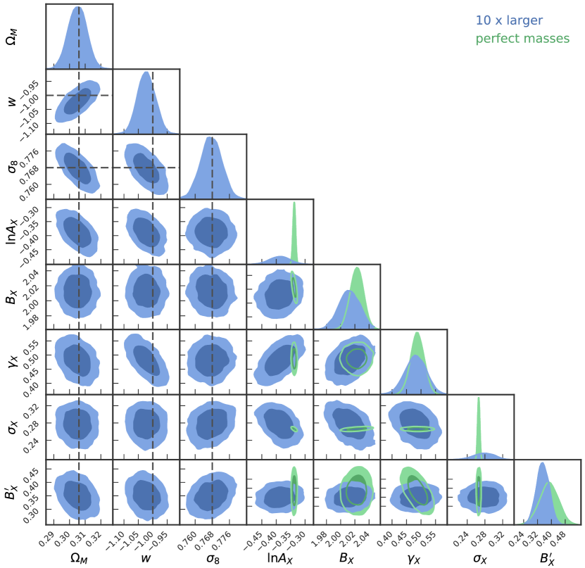
Figure 13: Posterior constraints of the number counts and the Euclid WL mass calibration of the 10 times larger validation mock (blue), and the constraints on the scaling relation parameters from the perfect masses mass calibration (green). All values are consistent within two sigma, indicating that our likelihoods are unbiased at a level which is small compared to the Poisson noise in our mock eROSITA sample.

To validated these likelihoods, we create a mock which is ten times larger than the eROSITA mock (by considering the unphysical survey footprint $\text{Area}_{\text{test}}=10\,\text{Area}_{\text{DE}}$). This leads to a reduction of the statistical uncertainties that enables us to better constrain systematic biases. We analyze this mock with the number counts and the Euclid WL mass calibration likelihood. We find that all parameters are consistent with the input values within less then two sigma. Scaling this up to the normal sized mock, we conclude that our code is unbiased at or below $\sim{2\over 3}$ sigma. We present for inspection a plot showing the results of the validation run as Fig. 13 at the end of the paper. The plot shows the marginal contours of the posterior distributions for the parameters with the input values marked.

Given that our mock catalog is a random realization of the stochastic processes modeled by the above described likelihoods, and that these likelihoods retrieve the input values even for a ten times larger mock, we take the liberty to shift best fit parameter values of the posterior samples presented in the following sections. These shifts are of the order of one sigma. Putting all posteriors to the same central value allows us to highlight the improvement of constraining power visible in the shrinking of the contours.

3.3 Comments on sampling and model choice

Various combinations of the above described likelihood functions are sampled using pymultinest (Buchner et al., 2014), a python wrapper of the nested sampling code multinest (Feroz et al., 2009). Nested sampling was originally developed to compute the evidence, or marginal likelihood, but has the added advantage of providing a converged posterior sample in the process (Skilling, 2006).

The parameters we sample depend on the specific application. In all cases considered, we sample the parameters of the X-ray selection scaling relation: $(\ln A_{\text{X}},B_{\text{X}},\gamma_{\text{X}},\sigma_{\text{X}},B_{\text{X}}^{\prime})$. When the WL mass calibration likelihood is sampled in Section 4.2, also the parameters governing the WL mass scaling relation are sampled: $(b_{\text{WL}},\sigma_{\text{WL}})$.

We explore two different flat cosmological models: (1) $\nu$-$\Lambda$CDM, and (2) $\nu$-$w$CDM. For both, we consider the following parameters: $H_{\text{0}}$, the current expansion rate of the Universe in units of km s^-1 Mpc^-1; $\omega_{b}$, the current day co-moving density of baryons w.r.t. the critical density of the Universe; $\Omega_{M}$, the current day density of matter w.r.t. the critical density; $A_{\text{S}}$, the amplitude of primordial curvature fluctuations; $n_{\text{S}}$, the spectral index of primordial curvature fluctuations; and the sum of neutrino masses $\sum m_{\nu}$ in eV.

The cosmological model where only these parameters are allowed to vary is called $\nu$-$\Lambda$CDM, because we allow for massive neutrinos of yet unknown mass, and assume that the agent of the late time accelerated expansion is a cosmological constant $\Lambda$.

As a more complex model $\nu$-$w$CDM, we also consider the case that the late time acceleration is not caused by the cosmological constant, but by an as yet unknown form of energy, usually referred to as dark energy. The properties of dark energy are described here by a single equation of state parameter $w$.

For better comparison, with other Large Scale Structure experiments, in both models, we also compute $\sigma_{8}$, the root mean square of linear matter fluctuations in a spherical region of 8 h^-1Mpc radius, as a derived quantity in each step of the chain and present the posterior distribution in this quantity rather than in the primordial power spectrum fluctuation amplitude $A_{\text{S}}$.

3.4 Choice of priors

Table 2: Priors used in our analysis. $\mathcal{U}(a,b)$ is a uniform flat prior in the interval $(a,b)$, $\ln\mathcal{U}(a,b)$ a uniform flat prior in log space, $\mathcal{N}(\mu,\sigma^{2})$ refers to a Gaussian distribution with mean $\mu$ and variance $\sigma^{2}$, $\mathcal{N}_{>a}(\mu,\sigma^{2})$ to a Gaussian distribution truncated for values smaller than $a$.
Comment: a) Numerical stability when computing the equations (9, 11, 12 and 15), requires the scatter to be larger than the sampling size of the numerical integrals.

Cosmology for Number counts w/o CMB
$H_{\text{0}}$	$\mathcal{U}(40,120)$	cf. Section 3.4.3
$\omega_{\text{b}}$	$\mathcal{U}(0.020,0.024)$
$\Omega_{\text{M}}$	$\mathcal{U}(0.1,0.5)$
$A_{\text{S}}$	$\ln\mathcal{U}(0.6\text{e}-9,2.5\text{e}-9)$
$n_{\text{S}}$	$\mathcal{U}(0.94,1.0)$
$\sum m_{\nu}[eV]$	$\mathcal{U}(0.,1.)$
$w$	$\mathcal{U}(-1.6,-0.6)$
Cosmology for Number counts w/ CMB
	cf. Section 3.4.3
X-ray Selection Scaling Relation
$\ln A_{\text{X}}$	$\mathcal{N}(-0.33,0.23^{2})$	cf. Appendix B
$B_{\text{X}}$	$\mathcal{N}(2.00,0.17^{2})$
$\gamma_{\text{X}}$	$\mathcal{N}(0.45,0.42^{2})$
$\sigma_{X}$	$\mathcal{N}_{>0.1}(0.28,0.11^{2})$	a)
$B_{\text{X}}^{\prime}$	$\mathcal{N}(0.36,0.78^{2})$
DES/HSC WL
$b_{\text{WL}}$	$\mathcal{N}(0.94,0.051^{2})$	cf. Section 3.4.2
$\sigma_{\text{WL}}$	$\mathcal{N}_{>0.1}(0.24,0.02^{2})$	a)
Euclid WL
$b_{\text{WL}}$	$\mathcal{N}(0.94,0.013^{2})$	cf. Section 3.4.2
$\sigma_{\text{WL}}$	$\mathcal{N}_{>0.1}(0.24,0.008^{2})$	a)
LSST WL
$b_{\text{WL}}$	$\mathcal{N}(0.94,0.015^{2})$	cf. Section 3.4.2
$\sigma_{\text{WL}}$	$\mathcal{N}_{>0.1}(0.24,0.008^{2})$	a)

In general, any Bayesian analysis, and more specifically pymultinest, requires the specification of priors for all parameters one intends to sample. In the following, we present our choice of priors. If the parameter is not mentioned below, it has a uniform prior in a range that is larger than the typical posterior uncertainties of that parameter. The prior choices are summarized in Table 2.

3.4.1 Current priors on scaling relation

As mentioned above– and discussed in detail in Appendix B– the eROSITA count rate scaling relation is described by five parameters: $(\ln A_{\text{X}},B_{\text{X}},\gamma_{\text{X}},\sigma_{\text{X}},B_{\text{X}}^{\prime})$. We put Gaussian priors on these parameters. The mean values are obtained in Section B.1 by determining the maximum likelihood points of the mass calibration likelihood when using perfect masses. The corresponding uncertainties in the priors are taken to match the uncertainties on the respective parameters presented in Table 5 of Bulbul et al. (2019) for the core included 0.5-2.0 keV luminosity-mass-redshift relation when fit with the scaling relation of Form II. These parameter uncertainties were extracted using a sample of 59 SPT selected galaxy clusters observed with XMM-Newton together with the SPT SZE-based halo masses calculated using the calibration from de Haan et al. (2016, see Table 3 results column 2).

When we extract cosmological constraints only with these priors (i.e., without any WL information) we consider that a “baseline” result representing a currently achievable knowledge of the parameters of the eROSITA rate-mass relation.

3.4.2 Priors on WL calibration

The priors on the parameters of the WL mass – halo mass relation reflect the understanding of both the observational and theoretical systematics of the WL mass calibration. In this work, we consider, the following sources of systematic uncertainty:

1. the accuracy of the shape measurement in the optical survey parameterized as the uncertainty on the multiplicative shear bias $\delta m$,

2. the systematic mis-estimation of the lensing efficiency $\langle\beta\rangle$ due to the bias in the photometric redshift estimation $b_{\hat{z}}$,

3. the uncertainty in the estimation of the contamination by cluster members $f_{\text{cl}}$ which results from the statistical uncertainty of the photometric redshifts $\sigma_{\hat{z}}$ and the background galaxy selection,

4. the statistical uncertainty with which the theoretical bias and scatter of the WL mass $\delta b_{\text{WL, sim}}$, and $\delta\sigma_{\text{WL, sim}}$, respectively, can be constrained with large structure formation simulations.

The first three effects do not directly induce a bias in the mass estimation, but affect the NFW fitting procedure. To estimate their impact on the WL mass estimate, we consider a shear profile for WL mass $3\times 10^{14}$ M_☉ and $z=0.4$, add the systematic shifts, and fit for the mass again. The difference in input and output masses is then taken as the WL mass systematic uncertainty induced by these effects. This technique provides an overall estimate of the systematic uncertainty level, while ignoring potential dependences on cluster redshift and mass.

For DES, we assume $\delta m=0.013$ (Zuntz et al., 2018). The bias on the photometric redshift estimation of the source galaxies is $b_{\hat{z}}=0.02$ (Cooke et al., 2014) which, considering the source redshift distribution of DES (cf. Section 2.2), leads to an uncertainty on the lensing efficiency $\delta\langle\beta\rangle=0.02$. For the uncertainty on the contamination, we project $\delta f_{\text{cl}}=0.01$ based on Dietrich et al. (2019). Taken all together, these uncertainties propagate to a WL mass uncertainty of $\delta b_{\text{WL, obs, DES}}=0.045$.

The current uncertainty on the theoretical WL mass bias is $\delta b_{\text{WL, sim, to day}}=0.05$ in Dietrich et al. (2019), when considering the effects of halo triaxiality, morphological variety, uncertainties in the mass-concentration relation and mis-centering. Due to larger available simulations (Lee et al., 2018), a better measurement of the mis-centering distribution and an improvement of the understanding of the mass– concentration relation, for DES we project a reduction of this uncertainty by a factor 2, yielding $\delta b_{\text{WL, sim, DES}}=0.025$. The same scaling is applied to the uncertainty on the scatter, yielding $\delta\sigma_{\text{WL, DES}}=0.02$.

Given the level of observational uncertainty, this projection can also be read as a necessity to improve the understanding of the theoretical biases. The estimates above provide a total uncertainty of the bias of the WL mass

$$\begin{split}\delta b_{\text{WL, DES}}&=\sqrt{b_{\text{WL, sim, DES}}^{2}+b_{\text{WL, obs, DES}}^{2}}\\ &=0.051,\end{split}$$ (17)

and an uncertainty on the scatter of the WL mass $\delta\sigma_{\text{WL, DES}}=0.02$. This amounts to a $5.1\%$ mass uncertainty from systematic effects, which is a conservative assumption, given that McClintock et al. (2019) already achieved such a level of systematics control for DES cluster mass calibration. For sake of simplicity, we assume that the final level of systematics in HSC is of the same as in DES. This assumption will be inadequate for the actual analysis of the data. We postpone the discussion about the difference between the analysis methods to the respective future works.

The specifications for Euclid are given in Laureijs et al. (2011). The requirement for the shape measurement is $\delta m=0.001$. For the bias on the photometric redshift estimation, the requirement is $b_{\hat{z}}=0.002$, which translates into $\delta\langle\beta\rangle=0.0014$. For the projection of the uncertainty on the contamination, we assume that in the case of DES it has equal contribution from (1) the number of clusters used for to characterize it and (2) the photometric redshift uncertainty. Thus, for Euclid we estimate

$$\begin{split}\delta f_{\text{cl, Eu}}^{2}&=\frac{\delta f_{\text{cl, DES}}^{2}}{2}\frac{N_{\text{DES}}}{N_{\text{Eu}}}+\frac{\delta f_{\text{cl, DES}}^{2}}{2}\left(\frac{\sigma_{\hat{z}\text{, Eu}}}{\sigma_{\hat{z}\text{, DES}}}\right)^{2}\\ &=0.0065^{2},\end{split}$$ (18)

where $N_{\text{DES}}\approx 3.8$k, and $N_{\text{Eu}}\approx 6.4$k, are the number of clusters with DES and Euclid shear information in our catalog (cf. Section 2.2), $\sigma_{\hat{z}\text{, Eu}}=0.06$ is the photometric redshift uncertainty for Euclid (Laureijs et al., 2011), and $\sigma_{\hat{z}\text{, DES}}=0.1$ is the photometric redshift uncertainty for DES (Sánchez et al., 2014). Taking all the above mentioned values together, we find $\delta b_{\text{WL, obs, Eu}}=0.0085$ for Euclid. To match this improvement in data quality, we project an improvement in the understanding of the theoretical biases by a factor of 5, providing $\delta b_{\text{WL, sim, Eu}}=0.01$, and $\delta\sigma_{\text{WL, Eu}}=0.008$. Thus, the total uncertainty on the WL mass bias for Euclid is

$$\delta b_{\text{WL, Eu}}=0.013.$$ (19)

The specifications for LSST systematics are summarized in LSST DESC et al. (2018). The requirement for the shape measurement is $\delta m=0.003$, while the requirement for the bias on the photometric redshift estimation $b_{\hat{z}}=0.001$, leading to $\delta\langle\beta\rangle=0.0007$. Using $N_{\text{LSST}}\approx 11$k, and $\sigma_{\hat{z}\text{, LSST}}=0.02$, we find an uncertainty on the cluster member contamination of $\delta f_{\text{cl, LSST}}=0.0044$. Summing all the above mentioned values together, we get $\delta b_{\text{WL, obs, LSST}}=0.011$. We project the same understanding in theoretical systematics for LSST as for Euclid. Thus, the total uncertainty on the WL mass bias for LSST is

$$\delta b_{\text{WL, LSST}}=0.015.$$ (20)

These values are adopted throughout this work as priors for the WL mass scaling relation parameters, as summarized in Table 2. We note that the effort required to theoretically constrain the WL bias and scatter parameters with this accuracy is considerable.

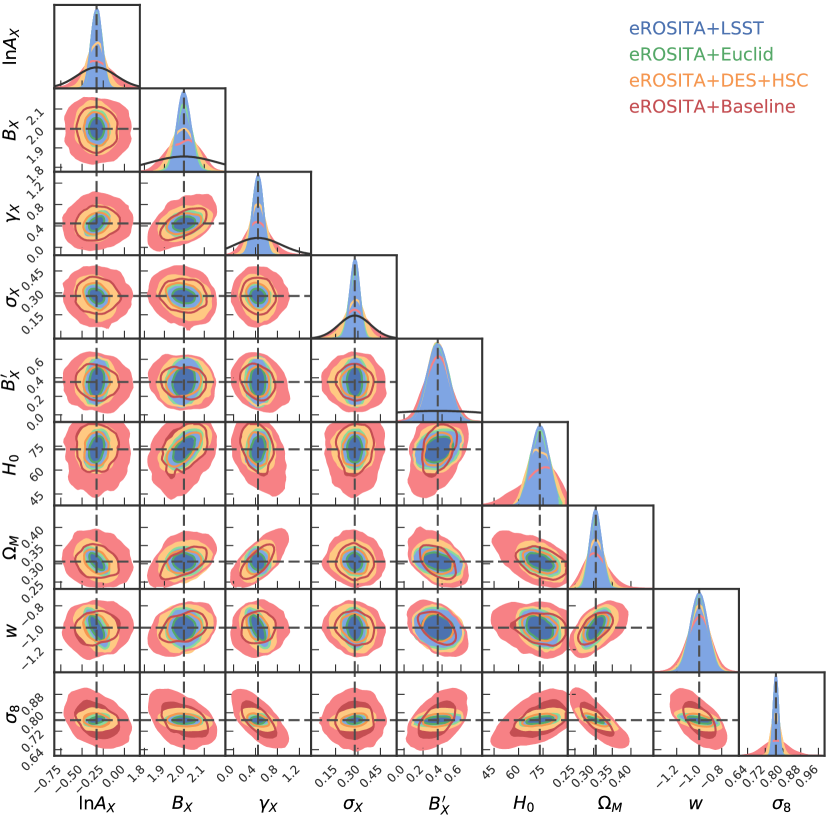
Figure 3: Predicted constraints on the scaling relation and cosmological parameters in $w$CDM. In red the constraints from the number counts alone (eROSITA+Baseline), in orange the constraints from number counts and DES+HSC WL calibration (eROSITA+DES+HSC), in green number counts and Euclid WL calibration (eROSITA+Euclid), and in blue number counts and LSTT WL calibration (eROSITA+LSST). The median values, all statistically consistent with the input values, are shifted to the input values to better highlight the increase in constraining power.

3.4.3 Cosmological priors

When sampling the number counts likelihood, we assume flat priors on all cosmological parameters except for $A_{\text{S}}$, for which we use a flat prior in log-space, as is good practice for strictly positive amplitudes. Similarly, we use priors on $\Omega_{\text{M}}$, $H_{\text{0}}$ and $w$ that are larger than the typical uncertainties on these parameters. For $\sum m_{\nu}$ we only explore the regime up to 1 eV, as current cosmological measurements, such as Planck Collaboration et al. (2016a) give upper limits on the summed neutrino mass around and below that value.

For $\omega_{b}$ and $n_{\text{S}}$ we use tight flat priors around the measured values of these parameters by the CMB experiments (Planck Collaboration et al., 2016a) and Big Bang Nucleosynthesis constraints derived from deuterium abundances (Cooke et al., 2014). We confirm that cluster number counts are not sensitive to these parameters within these tight ranges (Bocquet et al., 2018). It is thus not necessary to use informative priors on these parameters, as previous studies have done (see for instance Bocquet et al., 2015; de Haan et al., 2016).

In Section 4.3 we will consider the synergies between eROSITA number counts and WL mass calibration, and CMB temperature and polarization anisotropy measurements, which to date provide us with a significant amount of information about the cosmological parameters. In the models of interest, where either $w$ or $\sum m_{\nu}$ are free parameters, the CMB constraints from the Planck mission (Planck Collaboration et al., 2016a) display large degeneracies between the parameters we choose to sample. For this reason, we cannot approximate the CMB posterior as a Gaussian distribution. To capture the non-Gaussian feature, we calibrate a nearest-neighbor kernel density estimator (KDE) on the publicly available posterior sample. We utilize Gaussian kernels and, for each model, we tune the bandwidth through cross calibration to provide maximum likelihood of the KDE on a test subsample. As discussed in Section 2.3, our choice of input cosmology is slightly inconsistent with the CMB constraints. As we are only interested in the reduction of the uncertainties when combining CMB and eROSITA, we shift the CMB posteriors so that they are consistent with our input values at less than one sigma. The resulting estimator reproduces the parameter uncertainties and the degeneracies accurately.

4 Results

In the following subsections we first calculate how accurately the observable–mass scaling relation parameters must be constrained to enable the best possible cosmological constraints from the sample (Section 4.1). Thereafter we explore the impact of the WL mass calibration on the cosmological constraints that can be extracted from an analysis of the eROSITA galaxy cluster counts (Section 4.2). In Section 4.3 we explore synergies of the eROSITA dataset with the CMB and in Section 4.4 we examine the impact of combining the eROSITA dataset with BAO measurements from DESI. In Section 4.5 we examine the constraints derived when combining with both these external data sets, and the final subsection focuses on the impact of an eROSITA sample where the minimum mass is allowed to fall from our baseline value of $M_{500\text{c}}\goa 2\times 10^{14}\text{M}_{\sun}$ to $M_{500\text{c}}\goa 5\times 10^{13}\text{M}_{\sun}$, corresponding to a sample that is $\sim 3.5$ times larger.

4.1 Optimal mass calibration

The number counts likelihood depends both on the scaling relation parameters, and– through the mass function, the cosmological volume and their changes with redshift– also on the cosmological parameters. Furthermore, there are significant degeneracies between the mass scale of the cluster sample (i.e., the parameters of the observable mass relation) and the cosmological parameters, as demonstrated already in the earliest studies (Haiman et al., 2001). A full self-calibration of the number counts (i.e., including no direct mass measurement information) that allows full cosmological and scaling relation freedom, results in only very weak cosmological constraints (e.g., Majumdar & Mohr, 2003, 2004). Thus, before forecasting the cosmological constraints from the eROSITA sample, we estimate how accurate the mass calibration needs to be so that the information contained in the number counts is primarily resulting in the reduction of uncertainties on the cosmological parameters rather than the observable mass scaling relation parameters.

To estimate this required level of mass calibration, which we refer to as "optimal mass calibration", we quantify how much the number counts constrain the scaling relation parameters when the cosmological parameters are fixed to fiducial values. In such a case, all the information contained in the number counts likelihood informs our posterior on the scaling relation parameters. If this level of information, or more, were provided by direct mass calibration, then the number counts information would predominantly constrain the cosmology. In this sense, the optimal mass calibration then provides a threshold or goal for the amount and precision of external mass calibration we should strive for in our direct mass calibration through, e.g., weak lensing.

We find that in fact the number counts alone do not contain enough information to meaningfully constrain all five scaling relation parameters even in the presence of full cosmological information. Our scaling relation parametrization includes two additional parameters beyond those explored in Majumdar & Mohr (2003), the scatter $\sigma_{X}$ and the redshift evolution of the mass trend $B_{\text{X}}^{\prime}$. Thus, as a next test, we examine the constraints from number counts with fixed cosmology while assuming priors only on $B_{\text{X}}^{\prime}$. Interestingly, in this case we find that the constraints lead to an upper limit on the scatter of the scaling relation $\sigma_{X}<0.44$ (at $95\%$), which is weaker than our current knowledge of that parameter, which we infer from the scatter in the X-ray luminosity–mass relation from Bulbul et al. (2019, see discussions in Section 3.4 and Appendix B). We therefore adopt this external prior on the scatter parameter and allow full freedom for all other parameters (including $B_{\text{X}}^{\prime}$). Results in this case are more interesting, providing constraints that we adopt as our estimate of optimal mass calibration. The uncertainties are $\delta\ln A_{\text{X}}=0.042$, $\delta B_{\text{X}}=0.024$, $\delta\gamma_{\text{X}}=0.053$, and $\delta B_{\text{X}}^{\prime}=0.116$. We take this to mean that an optimal cosmological exploitation of the eROSITA cluster number counts will require that we know the parameters of the observable mass relation to at least these levels of precision. We will discuss in the following how this can be accomplished.

4.2 Forecasts: eROSITA+WL

Table 3: Forecast parameter constraints for eROSITA number counts with current, best available calibration (eROSITA+Baseline), with DES+HSC WL calibration (eROSITA+DES+HSC), with Euclid WL calibration (eROSITA+Euclid), and with LSST WL calibration (eROSITA+LSST) are presented in two different models, $\nu$-$w$CDM and $\nu$-$\Lambda$CDM within three different scenarios. From top to bottom they are eROSITA+WL alone, in combination with Planck CMB constraints (Pl15) and in combination with DESI BAO and Alcock-Pacynzki test constraints. Also shown are the scaling relation parameter uncertainties for an optimal mass calibration. In addition to the five cosmological parameters who constraints are presented, each model includes the parameters $n_{\mathrm{S}}$ and $\omega_{\mathrm{b}}$ marginalized over weak priors (see Table 2). The units of the column “$\sum m_{\nu}$” and “$H_{\text{0}}$” are eV and km s^-1 Mpc^-1, respectively. Comments: a) This parameter is not constrained within the prior ranges. When reporting upper limits “<”, we refer to the 95th percentile, while lower limits “>” refer to the 5th percentile. When a parameter is kept fixed in that model, we use “–”.

		$\Omega_{\text{M}}$	$\sigma_{8}$	$w$	$\sum m_{\nu}$	$H_{\text{0}}$	$\ln A_{\text{X}}$	$B_{\text{X}}$	$\gamma_{\text{X}}$	$\sigma_{\text{X}}$	$B_{\text{X}}^{\prime}$
optimal mass calibration							0.042	0.024	0.053		0.116
eROSITA + WL calibration
$\nu$-$w$CDM	priors						0.23	0.17	0.42	0.11	0.78
	eROSITA+Baseline	0.032	0.052	0.101	${}^{\text{a)}}$	10.72	0.165	0.073	0.209	0.083	0.128
	eROSITA+DES+HSC	0.023	0.017	0.085	${}^{\text{a)}}$	6.449	0.099	0.053	0.121	0.062	0.111
	eROSITA+Euclid	0.016	0.012	0.074	${}^{\text{a)}}$	5.210	0.059	0.037	0.090	0.034	0.107
	eROSITA+LSST	0.014	0.010	0.071	${}^{\text{a)}}$	4.918	0.058	0.031	0.089	0.030	0.107
$\nu$-$\Lambda$CDM	priors			–			0.23	0.17	0.42	0.11	0.78
	eROSITA+Baseline	0.026	0.033	–	${}^{\text{a)}}$	10.18	0.157	0.069	0.192	0.078	0.110
	eROSITA+DES+HSC	0.016	0.014	–	${}^{\text{a)}}$	5.664	0.091	0.049	0.103	0.059	0.104
	eROSITA+Euclid	0.011	0.007	–	${}^{\text{a)}}$	4.691	0.040	0.035	0.065	0.033	0.104
	eROSITA+LSST	0.009	0.007	–	${}^{\text{a)}}$	4.691	0.039	0.032	0.058	0.029	0.104
eROSITA + WL calibration + Pl15 (TTTEE_lowTEB)
$\nu$-$w$CDM	priors (incl. CMB)	<0.393	0.063	0.242	<0.667	>62.25	0.23	0.17	0.42	0.11	0.78
	eROSITA+Baseline	0.019	0.032	0.087	<0.590	2.857	0.165	0.026	0.132	0.083	0.121
	eROSITA+DES+HSC	0.018	0.019	0.085	<0.554	2.206	0.099	0.024	0.118	0.062	0.107
	eROSITA+Euclid	0.014	0.010	0.074	<0.392	1.789	0.059	0.020	0.090	0.034	0.107
	eROSITA+LSST	0.013	0.009	0.069	<0.383	1.662	0.058	0.018	0.080	0.030	0.103
$\nu$-$\Lambda$CDM	priors (incl. CMB)	0.024	0.035	–	<0.514	1.723	0.23	0.17	0.42	0.11	0.78
	eROSITA+Baseline	0.016	0.018	–	<0.425	1.192	0.122	0.025	0.101	0.077	0.110
	eROSITA+DES+HSC	0.013	0.015	–	<0.401	1.067	0.086	0.023	0.098	0.060	0.104
	eROSITA+Euclid	0.011	0.007	–	<0.291	0.978	0.039	0.020	0.065	0.033	0.103
	eROSITA+LSST	0.009	0.007	–	<0.285	0.767	0.038	0.020	0.054	0.030	0.103
eROSITA + WL calibration + DESI (BAO)
$\nu$-$w$CDM	priors (incl. BAO)	0.007	${}^{\text{a)}}$	0.086	${}^{\text{a)}}$	${}^{\text{a)}}$	0.23	0.17	0.42	0.11	0.78
	eROSITA+Baseline	0.007	0.030	0.063	${}^{\text{a)}}$	1.987	0.164	0.043	0.139	0.083	0.128
	eROSITA+DES+HSC	0.006	0.010	0.051	${}^{\text{a)}}$	1.597	0.086	0.037	0.110	0.056	0.101
	eROSITA+Euclid	0.006	0.005	0.047	${}^{\text{a)}}$	1.463	0.040	0.030	0.086	0.032	0.096
	eROSITA+LSST	0.006	0.005	0.043	${}^{\text{a)}}$	1.403	0.040	0.026	0.076	0.029	0.095
$\nu$-$\Lambda$CDM	priors (incl. BAO)	0.006	${}^{\text{a)}}$	–	${}^{\text{a)}}$	${}^{\text{a)}}$	0.23	0.17	0.42	0.11	0.78
	eROSITA+Baseline	0.006	0.015	–	${}^{\text{a)}}$	0.943	0.094	0.041	0.109	0.078	0.110
	eROSITA+DES+HSC	0.006	0.010	–	${}^{\text{a)}}$	0.925	0.074	0.040	0.077	0.055	0.104
	eROSITA+Euclid	0.006	0.005	–	${}^{\text{a)}}$	0.910	0.040	0.029	0.054	0.032	0.089
	eROSITA+LSST	0.006	0.005	–	${}^{\text{a)}}$	0.910	0.035	0.025	0.053	0.027	0.089
eROSITA + WL calibration + DESI + Pl15
$\nu$-$w$CDM	priors (incl. CMB+BAO)	0.007	0.027	0.049	<0.284	1.118	0.23	0.17	0.42	0.11	0.78
	eROSITA+Baseline	0.006	0.026	0.049	<0.281	1.103	0.161	0.023	0.079	0.083	0.128
	eROSITA+DES+HSC	0.006	0.011	0.048	<0.245	1.050	0.085	0.023	0.071	0.061	0.104
	eROSITA+Euclid	0.005	0.006	0.047	<0.241	1.023	0.039	0.017	0.064	0.032	0.095
	eROSITA+LSST	0.005	0.006	0.039	<0.223	0.870	0.038	0.017	0.064	0.029	0.089
$\nu$-$\Lambda$CDM	priors (incl. CMB+BAO)	0.004	0.020	–	<0.256	0.255	0.23	0.17	0.42	0.11	0.78
	eROSITA+Baseline	0.004	0.016	–	<0.254	0.253	0.093	0.024	0.067	0.074	0.110
	eROSITA+DES+HSC	0.004	0.009	–	<0.218	0.251	0.072	0.021	0.062	0.051	0.095
	eROSITA+Euclid	0.003	0.004	–	<0.211	0.148	0.035	0.020	0.050	0.033	0.071
	eROSITA+LSST	0.002	0.003	–	<0.185	0.145	0.033	0.017	0.050	0.033	0.069

4.2.1 $\nu$-$w$CDM constraints

As a first cosmological model we investigate $\nu$-$w$CDM, a flat cold Dark Matter cosmology with dark energy with constant but free equation of state parameter $w$ and massive neutrinos. In this Section, we present the constraints on the cosmological parameters for three different cases: number counts alone combined with baseline priors on the X-ray observable mass scaling relation that we derive from the latest analysis within SPT (Bulbul et al., 2019) (eROSITA+Baseline), number counts with DES+HSC WL mass calibration (eROSITA+DES+HSC), number counts with Euclid WL mass calibration (eROSITA+Euclid), and number counts with LSST WL mass calibration (eROSITA+LSST) . The respective marginal contour plot is shown in Fig. 3, and the corresponding uncertainties are listed in Table 3.

Considering the current knowledge of the X-ray scaling relation, we find that eROSITA number counts constrain $\Omega_{\text{M}}$ to $\pm 0.032$, $\sigma_{8}$ to $\pm 0.052$, $w$ to $\pm 0.101$, and $H_{\text{0}}$ to $\pm 10.72$ km s^-1 Mpc^-1, while marginalizing over the summed neutrino mass $\sum m_{\nu}<1$ eV without constraining it. We also find no constraints on $\omega_{\text{b}}$ and $n_{\text{S}}$ within the prior ranges that we assumed.

The addition of mass information consistently reduces the uncertainties on the cosmological parameters: the knowledge on $\Omega_{\text{M}}$ is improved by factors of $1.4$, $2.0$ and $2.3$ when adding DES+HSC, Euclid, and LSST WL information, respectively; for $\sigma_{8}$ the improvements are $3.1$, $4.3$ and $5.2$, whereas for the dark energy equation of state parameter they are $1.2$, $1.4$ and $1.4$, respectively. In summary, weak lensing calibration provides the strongest improvement of the determination of $\sigma_{8}$, followed by $\Omega_{M}$. The improvements on the dark energy equation of state parameter $w$ are clearly weaker.

4.2.2 $\nu$-$\Lambda$CDM constraints

We also investigate a model in which the equation of state parameter $w$ is kept constant: $\nu$ $\Lambda$CDM. The corresponding uncertainties are shown in Table 3. In this model, we find that the constraints on $\Omega_{\text{M}}$ and $\sigma_{8}$ are $0.019$ and $0.032$, respectively, which is tighter than in the $\nu$-$w$CDM model. However, the constraint on $H_{\text{0}}$ is comparable in the two models.

We also find that the addition of WL mass information improves the constraints on $\Omega_{\text{M}}$ by factors of $1.6$, $2.4$ and $2.9$ for DES+HSC, Euclid and LSST, respectively. The determination of $\sigma_{8}$ improves by factors $2.4$, $4.7$ and $4.7$. It is especially worth highlighting how eROSITA with Euclid or LSST WL information will be able to determine $\sigma_{8}$ at a sub-percent level. Nevertheless, also in this simpler model we find that eROSITA number counts do not constrain the summed neutrino mass in the sub-eV regime.

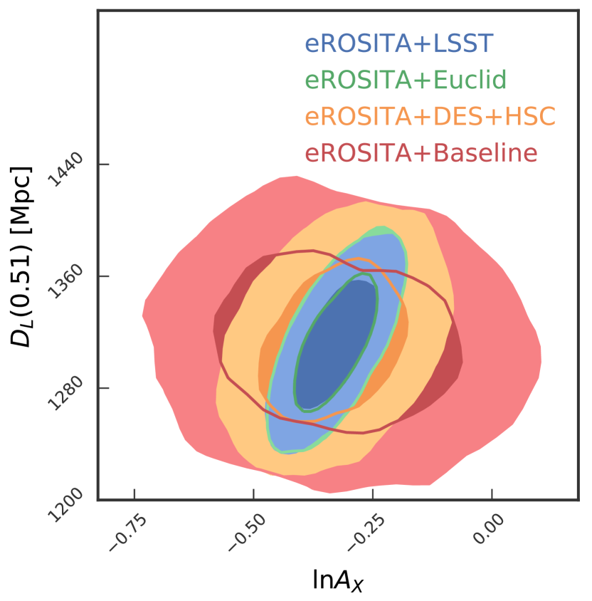
Figure 4: Two dimensional marginalized posterior sample of the amplitude of the scaling relation $A_{\text{X}}$ and the luminosity distance to the median redshift of our sample $D_{\text{L}}(0.51)$ in Mpc, as derived from the cosmological parameters in the posterior sample in the $w$CDM model. In red, orange, green and blue we present the constraints from the number counts alone (eROSITA+Baseline), from number counts and DES+HSC WL calibration (eROSITA+DES+HSC), Euclid WL calibration (eROSITA+Euclid), and LSST WL calibration (eROSITA+LSST), respecitvely. When no direct mass information is present, as in the case of number counts only, the two quantities are not degenerate with each other. As mass information is added, the underlying parameter degeneracy between the amplitude of the X-ray observable mass relation and the cosmological distance information emerges.

4.2.3 Limiting parameter degeneracy

We have studied the causes of the weaker improvement in $w$ when calibrating with Euclid or LSST WL, and we have discovered an interesting degeneracy due to the $w$ sensitivity of the distance. Remember that our WL calibration dataset consists of observations of the shear profiles and the redshift distributions of the background galaxies. To turn these into masses, one needs the cosmology sensitive angular diameter distances (see discussion below equation 5). Moreover, our selection observable is the eROSITA count rate (similar to X-ray flux) that is related to the underlying X-ray luminosity through the luminosity distance (see equation 7). This leads to a degeneracy between $w$, governing the redshift evolution of distances, and the amplitude and redshift trend of the selection observable–mass relation.

The degeneracy between $w$ and ($\ln A_{\text{X}}$, $\gamma_{\text{X}}$) can be easily understood by considering the parametric form of the rate mass scaling relation in equation (7). Ignore for a moment the distance dependence of the mass. Then for a given redshift $z$ and rate $\eta$, a shift in $w$ leads to a shift in the luminosity distance $D_{\text{L}}(z)$, and, to a minor degree, to a shift in the co-moving expansion rate $E(z)$. Such a shift can be compensated by a shift in $\ln A_{\text{X}}$ and $\gamma_{\text{X}}$, resulting in the same mass, and consequently the same number of clusters, making it indiscernible. The distance dependence of the shear to mass mapping and the power law dependence of the rate on mass leads to a somewhat different dependence, and so the parameter degeneracy is not catastrophic.

This effect is demonstrated in Fig. 4, where the joint posterior of the luminosity distance to the median cluster redshift $D_{\text{L}}(0.51)$ and of the amplitude of the scaling relation $\ln A_{\text{X}}$ is shown. In the case of no direct mass information, when we fit the number counts with priors on the scaling relation parameters, the median distance and the amplitude are uncorrelated. As one adds more mass information, e.g., the +DES-HSC WL, and +Euclid WL or +LSST WL cases, the underlying correlation between the median distance and the amplitude becomes apparent. This degeneracy provides a limitation to improving the $w$ constraint from the number counts by means of mass calibration. Given that it affects the halo masses directly, and not only the WL signal, we expect these degeneracies to be present also in other mass calibration methods, although to a different extent, given the different scaling of the selection observables with mass.

As a side note, these degeneracies highlight the importance of fitting for mass calibration and number counts simultaneously and self consistently. A mass calibration done at fixed cosmology would miss these correlations and lead to underestimated uncertainties on the scaling relation parameters. More worrisome, modeling mass calibration by simply adopting priors on the observable mass scaling relation parameters would miss the underlying physical degeneracies altogether (e.g., Sartoris et al., 2016; Pillepich et al., 2018).

The degeneracies between the distance redshift relation and the scaling relation parameters in the mass calibration explain why the impact of WL mass calibration in weaker in the $\nu$-$w$CDM model, compared to the $\nu$ $\Lambda$CDM model: in the latter $w$ is kept fixed, and the redshift evolution of distances and critical densities is controlled predominantly by a single variable: $\Omega_{\text{M}}$. With one degenerate degree of freedom less, WL mass calibration can put tighter constraints on $\ln A_{\text{X}}$ and $\gamma_{\text{X}}$ in the $\nu$-$\Lambda$CDM than in the $\nu$-$w$CDM model.

4.3 Synergies with Planck CMB

It is customary in observational cosmology to combine the statistical power of different experiments to further constrain the cosmological parameters. An important part of these improvements is due to the fact that each experiment has distinctive parameter degeneracies that can be broken in combination with constraints from another experiment. This is especially true for CMB temperature and polarization anisotropy measurements, which constrain the cosmological parameters in the early Universe, but display important degeneracies on late time parameters such as $\Omega_{\text{M}}$, $\sigma_{8}$ and $w$ (for a recent study applicable to current CMB measurements, see Howlett et al., 2012). We will discuss in the following the synergies between the Planck cosmological constraints from temperature and polarization anisotropy (Planck Collaboration et al., 2016a) and those from the eROSITA cluster counts analysis.

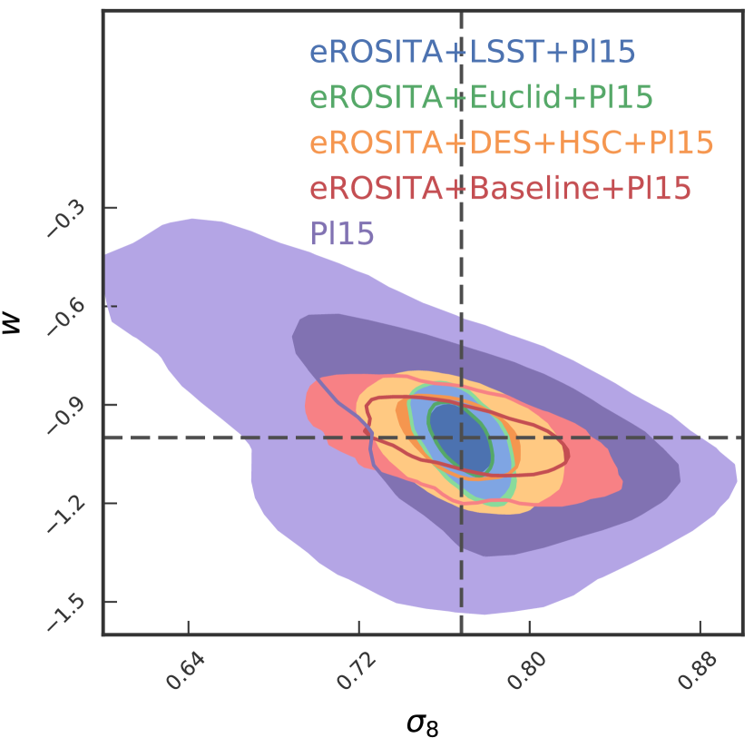
Figure 5: Marginalized posterior sample of $\sigma_{8}$ and $w$ in the $w$CDM model. In purple the constraints from Planck CMB alone (Pl15), in red the constraints from the number counts and Planck (eROSITA+Baseline+Pl15), in orange the constraints from the addition of DES+HSC WL calibration (eROSITA+DES+HSC+Pl15), in green for the addition Euclid WL calibration (eROSITA+Euclid+Pl15), in blue for the addition LSST WL calibration (eROSITA+LSST+Pl15). Cluster information breaks the inherent CMB degeneracies and allows to constrain the late time parameters to high precision.

4.3.1 $\nu$-$w$CDM constraints

In the $\nu$-$w$CDM model, the CMB suffers from the so called geometrical degeneracy (Efstathiou & Bond, 1999), that arises because the CMB anisotropy primarily constrains the ratio of the sound horizon at recombination and the angular diameter distance to that epoch. As a consequence, for example, the current day expansion rate $H_{\text{0}}$ is degenerate with the equation of state parameter $w$. This uncertainty in the expansion history of the Universe leads to large uncertainties on late time properties such as $\Omega_{\text{M}}$ and $\sigma_{8}$. Addition of a late time probe that constrains these quantities allows one to break the degeneracies and put tighter constraints on $w$. This can be nicely seen for the case of eROSITA in Fig. 5, where the red CMB degeneracy between $\sigma_{8}$ and $w$ is broken by the addition of cluster information. The corresponding uncertainties are shown in Table 3.

While in this model the CMB alone is not able to determine $\Omega_{\text{M}}$, the addition of eROSITA number counts allows a constraint of $\pm 0.019$. Inclusion of WL mass information further reduces the uncertainty to $0.018$, $0.014$ and $0.013$ for DES+HSC, Euclid and LSST, respectively. The uncertainty in $\sigma_{8}$ is reduced from $0.065$ when considering only the CMB, to $0.032$ with number counts, $0.019$ with number counts and DES+HSC WL, and $0.010$ with number counts and Euclid, and $0.009$ with LSST WL. Noticeably, the determination of the equation of state parameter $w$ is improved from $0.242$ from CMB data alone, to $0.087$ when adding number counts. Even more remarkable is the fact that WL calibrated eROSITA constraints on $w$ are only margimally improved by the addition of CMB information.

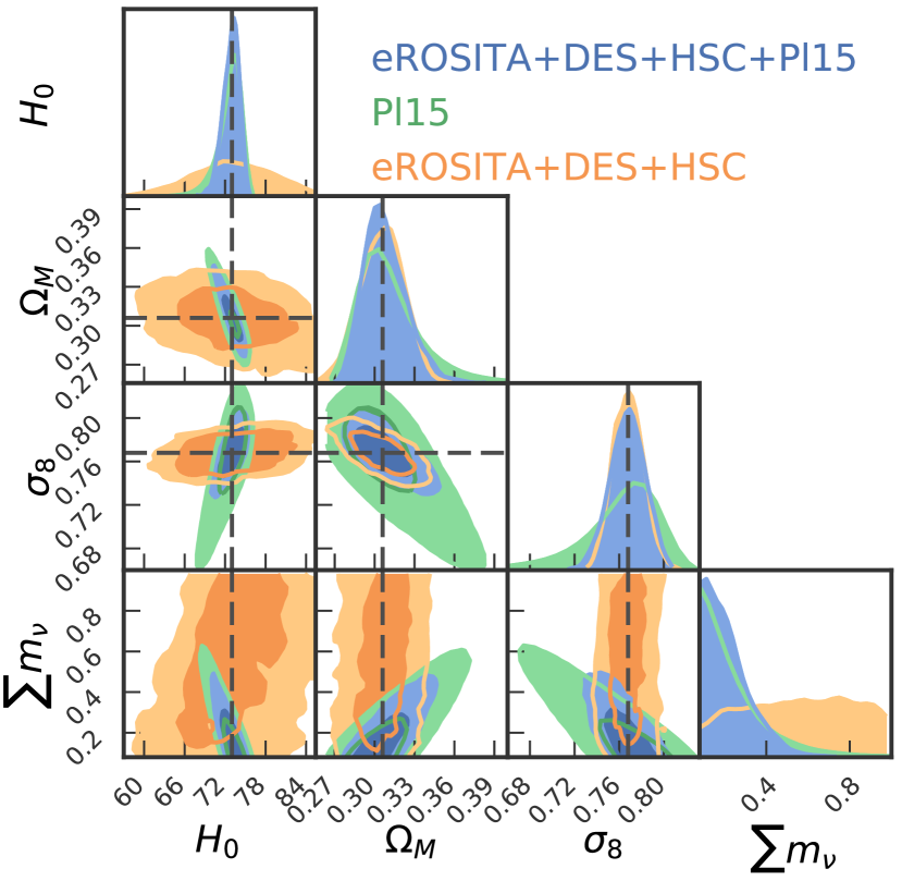
Figure 6: Marginalized posterior sample of $H_{\text{0}}$, $\Omega_{\text{M}}$, $\sigma_{8}$ and $\sum m_{\nu}$ in the $\nu$-$\Lambda$CDM model. In red the constraints from Planck CMB alone (Pl15) and the constraints from eROSITA number counts and DES WL calibration without CMB priors in blue (eROSITA+DES), and with CMB priors in purple (eROSITA+DES+Pl15). By measuring $\sigma_{8}$ and $\Omega_{\text{M}}$ independently of the sum of neutrino masses, WL calibrated cluster number counts break the degeneracy among these parameters in the CMB posteriors.

4.3.2 Constraints on sum of the neutrino masses

We showed earlier that cluster number counts, even when they are WL calibrated, provide little information about the sum of the neutrino masses in the regime $<1$ eV. On the other hand, the CMB posteriors on $\sigma_{8}$ and $\Omega_{\text{M}}$ are strongly degenerate with the neutrino mass, as can be seen in Fig. 6. Contrary to the CMB, the number counts of galaxy clusters are only weakly affected by the sum of the neutrino mass. Recent studies have shown that the halo mass function is a function of the power spectrum of baryons and dark matter only (Costanzi et al., 2013; Castorina et al., 2014). Effectively, this means that number counts can be used to constrain the density $\Omega_{\text{coll}}$ and fluctuation amplitude $\sigma_{8,\text{coll}}$ of baryons and dark matter independently of the neutrino mass. If one considers matter as cold dark matter, baryons and neutrinos, as is customarily done, then $\Omega_{\text{M}}=\Omega_{\text{coll}}+\Omega_{\nu}$ and $\sigma_{8}^{2}=\sigma_{8,\text{coll}}^{2}+\sigma_{8,\nu}^{2}$, where $\Omega_{\nu}$ is the density parameter of neutrinos and $\sigma_{8,\nu}^{2}$ is the amplitude of their clustering on 8$h^{-1}$ Mpc scales. The counts derived constraints on $\Omega_{\text{coll}}$ and $\sigma_{8,\text{coll}}$ then lead to only very weak degeneracies between the sum of the neutrino masses and $\Omega_{\mathrm{M}}$ and $\sigma_{8}$, respectively, because neutrinos constitute a tiny fraction of the total matter density and the total matter fluctuations on 8$h^{-1}$ Mpc scales. In Fig. 6 we can see how these very different parameter degeneracies in the CMB and cluster counts manifest themselves. Combining these weaker degeneracies arising from eROSITA+DES WL with the more pronounced degeneracies in the CMB posteriors allows us to break the latter and to better constrain the sum of the neutrino masses.

Consistently, we find that in the $\nu$-$\Lambda$CDM model, the addition of CMB priors only marginally improves the constraints eROSITA will put on $\sigma_{8}$ and $\Omega_{\text{M}}$. However, while the CMB alone puts an upper limit of $\sum m_{\nu}<0.514$ eV (at 95%) we determine that the combination of Planck CMB and eROSITA number counts will constrain the neutrino masses to $<0.425$ eV, which will improve to $<0.401$ eV, $<0.291$ eV and $<0.285$ eV with the addition of WL information from DES+HSC, Euclid and LSST, respectively.

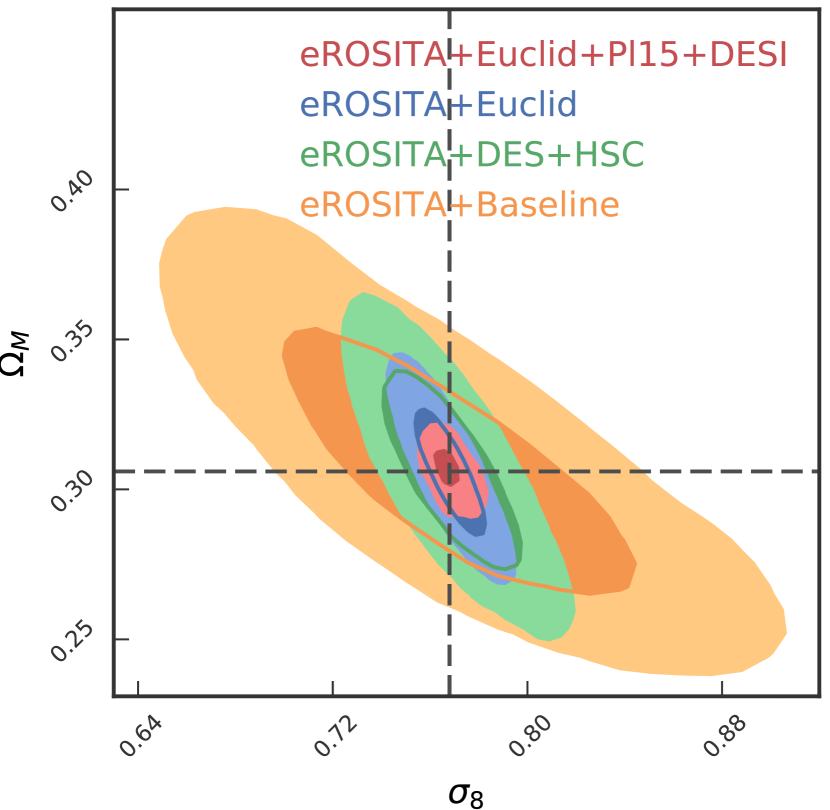
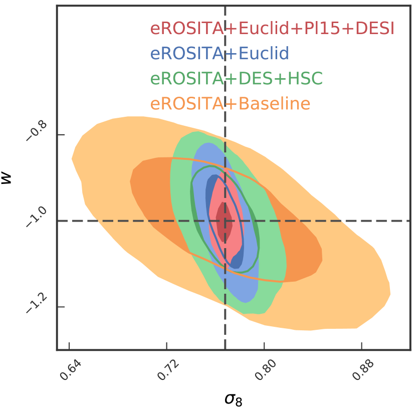
Figure 7: 2 dimensional marginal contours of the posteriors in ($\Omega_{\text{M}}$,$\sigma_{8}$) (left panel) and ($w$,$\sigma_{8}$) (right panel), showing the incremental improvement of constraining power when first adding WL information and second combining with external cosmological data sets (“Pl15” stands for the CMB fluctuation measurements by the Planck satellite, while “DESI” refers only to the BAO constraints). These posteriors are derived while simultaneously marginalizing over the summed neutrino mass.

4.4 Synergies with DESI BAO measurements

From the discussion in Section 4.2.3, it is apparent that the flux based X-ray selection and the distance dependent WL mass information lead to an inherent degeneracy between distances to the clusters and scaling relation parameters that ultimately limits the constraint on $w$. It would be desirable to utilize CMB independent constraints on the distance redshift relation, to allow for more stringent consistency checks between cluster derived constraints and CMB constraints. Some previous cosmological studies of X-ray clusters have used the distance information gleaned from the assumption of constant intracluster medium (ICM) mass fraction with redshift (Mantz et al., 2015; Schellenberger & Reiprich, 2017). While these results are encouraging, a challenge with this method is that it only provides accurate distance information if in fact the ICM mass fraction is constant at all redshifts. It has been established for decades now that the ICM mass fraction varies with cluster mass (e.g., Mohr et al., 1999), but direct studies of how the ICM mass fraction varies over the redshift range of the eROSITA survey (i.e., extending beyond $z=1$) have only recently been undertaken (Lin et al., 2012; Chiu et al., 2016, 2018; Bulbul et al., 2019). The evolution is consistent with constant ICM mass fraction, but the uncertainties are still large. Further study is clearly needed. Another interesting eROSITA internal prospect for better constraining the distance redshift relation is to utilize the clustering of clusters to determine the BAO scale (for a recent application, see Marulli et al., 2018, and references therein.)

As an alternative, we consider constraints from other low redshift experiments, more precisely the measurement of the Baryonic Acoustic Oscillations (hereafter BAO) in future spectroscopy galaxy surveys. In this work, we consider the forecast for the constraints provided by the Dark Energy Spectroscopy Instrument (DESI; Levi et al., 2013) as the relative error on the transversal BAO measurement $d_{\mathrm{A}}/r_{\text{S}}$ and the radial BAO measurement $H(z)\,r_{\text{S}}$ as functions of redshift, where $d_{\mathrm{A}}$ is the angular diameter distance, $H(z)$ the expansion rate, and $r_{\text{S}}$ is the sound horizon. The values adopted in this work are reported in Table V of Font-Ribera et al. (2014). Furthermore, we follow the authors indications and assume that in each redshift bin, the measurement error on the two quantities are correlated with correlation coefficient $\rho=0.4$. Using this information we perform an importance sampling of the posterior samples presented above and summarize the resulting uncertainties in Table 3.

When considering the uncertainties on the different parameters obtained by sampling these observables, we find that the BAO measurement dominates the uncertainty on $\Omega_{\text{M}}$. The addition of number counts, or number counts and WL information does not lead to major improvements on this parameter either in $\nu$-$w$CDM or in $\nu$-$\Lambda$CDM. However, the uncertainty on the dark energy equation of state parameter $w$ is reduced from $0.086$ in the BAO only case, to $0.065$ when adding just number counts, $0.054$ and $0.047$ when adding DES+HSC and Euclid WL information, respectively. Remarkably, eROSITA counts with BAO priors on the expansion history outperforms eROSITA counts with CMB priors when it comes to constraining the parameters $\Omega_{\text{M}}$, $\sigma_{8}$ and $w$, while simultaneously marginalizing over the summed neutrino mass. The latter is unconstrained by eROSITA+BAO, even when considering WL mass information. Furthermore, eROSITA+BAO allows us to measure the Hubble constant $H_{\text{0}}$ to varying degrees of precision, depending on the quality of the WL data. While these constraints never go below the present precision from other methods (see for instance Riess et al., 2016), they will provide a valuable systematics cross-check (for an example of systematics in SNe Ia that impact local $H_{0}$ measurements, see, e.g., Rigault et al., 2013, 2015, 2018).

4.5 Combining all datasets

It is current practice in cosmology to first test consistency of constraints from different data sets as a check on systematics and to then combine the constraints as possible to provide the most precise cosmological parameter constraints possible. In the case of a forecast work like this, agreement is guaranteed by the choice of input cosmology for the mock creation, while statistical independence can be assumed for eROSITA with WL data, DESI and the CMB measurement from Planck.

We provide the results of this combination at the bottom of Table 3. In $\nu$-$w$CDM, already the combination of Planck CMB measurements and DESI BAOs allows us to determine $\Omega_{\text{M}}$ and $w$ to $0.007$ and $0.049$, respectively, while simultaneously putting an upper limit of $<0.284$ eV on the summed neutrino mass. Addition of eROSITA+Euclid WL only marginally improves these constraints to $0.005$ and $0.047$ for $\Omega_{\text{M}}$ and $w$, respectively, and leads to the 95% confidence upper limit $\sum m_{\nu}<0.241$ eV. In this configuration, however, the added value of eROSITA number counts and WL mass calibration lies in the ability to constrain $\sigma_{8}$: while CMB and BAO put a constraint of $0.027$, addition of eROSITA improves this to $0.026$, $0.011$ and $0.006$, when considering the baseline mass information, DES+HSC WL, Euclid WL or LSST WL, respectively. In summary, using BAO and CMB priors together increases the constraining power of eROSITA cluster cosmology considerably, as can be seen in the shrinking of the 2 dimensional marginal contours in ($\Omega_{\text{M}}$,$\sigma_{8}$) and ($w$,$\sigma_{8}$) space, shown in the left and the right panel of Fig. 7, respectively.

4.6 Inclusion of low mass clusters and groups

In this work, we have taken the conservative approach of excluding all systems with a halo mass $\loa 2\times 10^{14}\text{M}_{\sun}$ by means of increasing the eROSITA cluster count rate threshold at low redshift (cf. Section 2.1 and Appendix A). There are several good reasons to do so, all of them related, in one way or another, to an increase in systematic uncertainty when going to lower mass systems that are not as well studied. However, to enable comparison to previous work, and as a motivation to further investigate and control the systematic uncertainties in low mass clusters and groups, we also examine the impact of WL mass calibration on the constraining power for a cluster sample where the count rate threshold is reduced at low redshift so that only clusters with masses $M_{\text{500c}}\lessapprox 5\times 10^{13}\text{M}_{\sun}$ are excluded.

Table 4: Parameter uncertainties, for number counts (eROSITA+Baseline), number counts and DES+HSC WL calibration (eROSITA+DES+HSC), number counts and Euclid WL calibration (eROSITA+Euclid), and number counts and LSST WL calibration (eROSITA+LSST) in the $\nu$-$w$CDM model when including low mass clusters. The units of the column “$\sum m_{\nu}$” and “$H_{\text{0}}$” are eV and km s^-1 Mpc^-1, respectively. Comments: a) This parameter is not constrained within the prior ranges. When reporting upper limits “<”, we refer to the 95th percentile, while lower limits “>” refer to the 5th percentile. When a parameter is kept fixed in that model, we use “–”.

		$\Omega_{\text{M}}$	$\sigma_{8}$	$w$	$\sum m_{\nu}$	$H_{\text{0}}$	$\ln A_{\text{X}}$	$B_{\text{X}}$	$\gamma_{\text{X}}$	$\sigma_{\text{X}}$	$B_{\text{X}}^{\prime}$
optimal mass calibration							0.028	0.021	0.050		0.116
eROSITA + WL
$\nu$-$w$CDM	priors						0.23	0.17	0.42	0.11	0.78
	eROSITA+Baseline	0.025	0.038	0.079	${}^{\text{a)}}$	8.081	0.113	0.071	0.202	0.078	0.086
	eROSITA+DES+HSC	0.012	0.012	0.069	${}^{\text{a)}}$	4.572	0.081	0.028	0.097	0.052	0.072
	eROSITA+Euclid	0.009	0.007	0.056	${}^{\text{a)}}$	3.762	0.042	0.019	0.073	0.027	0.058
	eROSITA+LSST	0.007	0.006	0.050	${}^{\text{a)}}$	2.707	0.042	0.016	0.068	0.023	0.051
eROSITA + WL + Pl15 (TTTEE_lowTEB)
$\nu$-$w$CDM	priors (incl. CMB)	<0.393	0.063	0.242	<0.667	>62.25	0.23	0.17	0.42	0.11	0.78
	eROSITA+Baseline	0.017	0.028	0.078	<0.580	2.745	0.131	0.026	0.128	0.083	0.087
	eROSITA+DES+HSC	0.010	0.012	0.069	<0.542	1.587	0.092	0.017	0.102	0.052	0.065
	eROSITA+Euclid	0.007	0.006	0.060	<0.381	1.401	0.046	0.013	0.076	0.021	0.054
	eROSITA+LSST	0.006	0.005	0.051	<0.365	1.317	0.045	0.012	0.065	0.021	0.050
eROSITA + WL + DESI (BAO)
$\nu$-$w$CDM	priors (incl. BAO)	0.007	${}^{\text{a)}}$	0.086	${}^{\text{a)}}$	${}^{\text{a)}}$	0.23	0.17	0.42	0.11	0.78
	eROSITA+Baseline	0.006	0.016	0.051	${}^{\text{a)}}$	1.703	0.136	0.036	0.090	0.068	0.070
	eROSITA+DES+HSC	0.006	0.009	0.048	${}^{\text{a)}}$	1.425	0.080	0.025	0.084	0.050	0.059
	eROSITA+Euclid	0.005	0.005	0.038	${}^{\text{a)}}$	1.379	0.036	0.016	0.063	0.021	0.050
	eROSITA+LSST	0.004	0.005	0.038	${}^{\text{a)}}$	1.303	0.036	0.014	0.061	0.021	0.049
eROSITA + WL + DESI + Pl15
$\nu$-$w$CDM	priors (incl. CMB+BAO)	0.007	0.027	0.049	<0.284	1.118	0.23	0.17	0.42	0.11	0.78
	eROSITA+Baseline	0.005	0.015	0.046	<0.279	1.114	0.134	0.022	0.079	0.067	0.067
	eROSITA+DES+HSC	0.005	0.010	0.044	<0.242	1.040	0.078	0.014	0.067	0.049	0.056
	eROSITA+Euclid	0.005	0.005	0.037	<0.237	1.015	0.039	0.012	0.058	0.021	0.049
	eROSITA+LSST	0.004	0.005	0.034	<0.224	0.790	0.039	0.010	0.053	0.021	0.047

4.6.1 Systematics of low mass clusters and groups

There are several important systematic concerns. For instance, Bocquet et al. (2016) find in a study using hydrodynamical structure formation simulations that for masses below $10^{14}\text{M}_{\sun}$, baryonic feedback effects reduce the halo mass function by up to 10% compared to halo mass functions extracted from dark matter only simulations. The magnitude of this effect depends on the feedback model, and therefore needs be treated as a systematic uncertainty in the cosmological modeling. The magnitude of this uncertainty awaits further study.

Baryonic feedback effects also impact the mass profiles of clusters. Lee et al. (2018) show how active galactic nuclei feedback induces a deficit of mass in the cluster center when compared to gravity only simulations. The partial evacuation of baryons is strong enough to modify also the matter profile. Lee et al. (2018) demonstrate how this effect impacts the WL bias $b_{\text{WL}}$ and the WL scatter $\sigma_{\text{WL}}$, making them mass dependent. Such effects will need to be taken into account, especially when considering lower mass systems.

Similarly, the thermodynamic structure of low mass systems, generally called groups, is more complex than for massive galaxy clusters, showing a larger impact of non gravitational physics (Eckmiller et al., 2011; Bharadwaj et al., 2014; Barnes et al., 2017). Lovisari et al. (2015) showed that the mass slope of the luminosity mass relation is significantly steeper for groups than for clusters. Schellenberger & Reiprich (2017) demonstrate how such a break in the power law might bias the cosmological results derived from an X-ray selected cluster sample. We have thus chosen the conservative approach of excluding these systems from our primary eROSITA forecasts, thereby reducing the sensitivity of the forecast cosmological parameter constraints to these important complications at low masses.

4.6.2 Improvement of the constraints

Nevertheless, the controlled environment of mock data analysis allows us to investigate how much constraining power could ideally be gained by lowering the mass limit if all the above described systematics where well understood and controlled. To this end, we select a low mass sample by imposing an observable selection with redshift that enforces $M_{500\text{c}}\goa 5\times 10^{13}\text{M}_{\sun}$, assuming that the scaling relation and the mass function used for the fiducial sample are still valid also at this lower mass scale. This increases the sample size to 43k clusters, with a median redshift $\bar{z}=0.31$ and a median halo mass of $\bar{M}_{500\text{c}}=1.4\times 10^{14}\text{M}_{\sun}$. The resulting constraints on the parameters of the $\nu$-$w$CDM model are shown in Table 4. The constraints both on the cosmological parameters, as well as on the scaling relation parameters show a strong improvement compared to those from the higher mass sample. For eROSITA number counts we determine that the uncertainty on $\Omega_{\text{M}}$, $\sigma_{8}$ and $w$ will be reduced by factors of $1.3$, $1.4$ and $1.3$, respectively. When calibrating masses with DES+HSC, we find improvements of factor $1.9$, $1.4$ and $1.2$, when considering Euclid the inclusion of low mass systems will reduce the uncertainties by $1.8$, $1.7$ and $1.3$, while using LSST leads to reductions by $2.0$, $1.7$ and $1.4$. In absolute terms, eROSITA including low mass systems, calibrated with Euclid will provide constraints on $\Omega_{\text{M}}$, $\sigma_{8}$ and $w$ of $0.009$, $0.007$ and $0.056$, respectively. We emphasize that these tight constraints can only be obtained if the aforementioned systematic effects are adequately controlled.

5 Discussion

The above presented results on the constraining power of the eROSITA cluster sample demonstrate its value as a cosmological probe. They also underline the crucial impact of WL mass calibration on the constraining power of cluster number counts. However, they also give some clear indications of how this impact manifests itself in detail.

In the following subsections we discuss first how the constraints on the scaling relation parameters are affected by the addition of better WL data, by the choice of the model and by the choice of cosmological priors, resulting in an assessment of the conditions under which we can attain an optimal mass calibration. We then determine the sensitivity of our observable to the different input parameters. Finally, we compare our prediction to the constraints from current and future experiments.

5.1 Impact of WL on scaling relation parameters

In the previous section we discussed in detail the impact of WL mass calibration on the eROSITA cosmological parameter constraints. Naturally, adding WL information will also improve the constraints on the scaling relation parameters. The resulting uncertainties are reported in Table 3. In the following, we will focus on two interesting aspects of these results: first, we assess under which circumstances eROSITA will be optimally calibrated; second, we comment on the constraints on the scatter in observable at fixed mass.

5.1.1 Which mass calibration is optimal?

In Section 4.1, we introduced the concept of the optimal mass calibration. Comparing the bounds on the parameter uncertainties derived there to the forecasts for DES+HSC, we find that, independent of the presence of external cosmological priors and in both models we consider, DES WL will not provide an optimal calibration of the eROSITA observable mass relation. Only the calibration of the mass slope $B_{\text{X}}$ when considering CMB and BAO data is an exception to this. This is not to say that, as shown above, the inclusion of DES+HSC WL information does not improve the cosmological constraints. It is to say that some part of the information contained in the number counts is used to constrain the scaling relation parameters instead of the cosmological parameters.

The optimal nature of the Euclid or LSST mass calibration is more subtle. When the dark energy equation of state parameter is kept fixed in the $\nu$-$\Lambda$CDM model, Euclid provides an optimal mass calibration on the amplitude of the scaling relation, both with and without external cosmological priors from CMB or BAO observations. However, in the $\nu$-$w$CDM model without external priors, Euclid or LSST WL does not constrain the scaling relation parameters optimally. The amplitude is calibrated optimally after the inclusion of BAO data. On the other hand, including CMB priors makes an optimal calibration of the mass trend possible. In the presence of dark energy with free but constant equation of state, the redshift slope is never calibrated optimally. Nevertheless, as demonstrated in the previous section, even in the limit of sub-optimal mass calibration, the eROSITA dataset provides cosmological information complementary to these other cosmological experiments. Furthermore, the calibration of the redshift trend could be improved by complementary direct mass calibration methods. At high redshift, the most promising options would be pointed observations of high-z clusters (Schrabback et al., 2018a, b) and CMB-WL calibration (Baxter et al., 2015; Planck Collaboration et al., 2016b; Baxter et al., 2018).

5.1.2 Scatter in the count rate to mass relation

One may imagine that the inclusion of low scatter mass proxies in the number counts and mass calibration analysis may tighten the constraints on the scatter and thereby reduce the uncertainties on the cosmological parameters. Our present work does not seem to support this hypothesis. First, we show that even an arguably weak constraint on the scatter can be considered an optimal calibration (cf. Section 4.1). In other words, even at fixed cosmology, the number counts are unable to constrain the scatter. Consequently, our ability to constrain the cosmology using the number counts is not expected to depend strongly on the knowledge of the scatter. This can also be seen by the fact that there is little correlation between the scatter and any other parameter of interest in the $\nu$-$w$CDM posterior sample, as shown in Fig. 3 and Fig. 10. We conclude that constraining the scatter to high precision, although of astrophysical interest, is not required to perform an optimal cosmological analysis.

Furthermore, our results indicate that DES+HSC, Euclid and LSST WL mass calibration will be able to determine the scatter to $0.062$, $0.034$, and $0.030$, respectively (see Table 3). This may seem surprising, because WL mass calibration has large observational uncertainties and a large intrinsic scatter when compared to typical low scatter mass proxies such as the ICM mass or temperature. However, the final constraining power stems in our analysis from the large number of cluster with WL information and the relatively small prior uncertainty on the intrinsic WL scatter $\sigma_{\text{WL}}$. In summary, given that the knowledge of the scatter does not impact the constraints on the cosmological parameters, and that WL mass calibration is able to constrain the scatter directly, it is not clear that a dedicated scatter calibration through the inclusion of low scatter mass proxies like the ICM mass will significantly impact eROSITA cluster cosmology constraints. Further study would be required to confirm this.

5.2 Parameter sensitivities

Figure 8: Sensitivity in terms of change in log likelihood of the number counts likelihood to various parameters as a function of redshift. From left to right, each panel represents a higher count rate bin. The total number of clusters for the fiducial parameter values is shown as a dashed line. The parameters are varied from the fiducial values as noted at the top of the figure. The grey area shows the redshift range where we exclude low mass clusters by raising the selection threshold. Notably, we find that the number counts likelihood is most sensitive to the parameters $\Omega_{\text{M}}$ and $A_{\text{S}}$ with comparable sensitivity to $w$ and $A_{\text{X}}$.

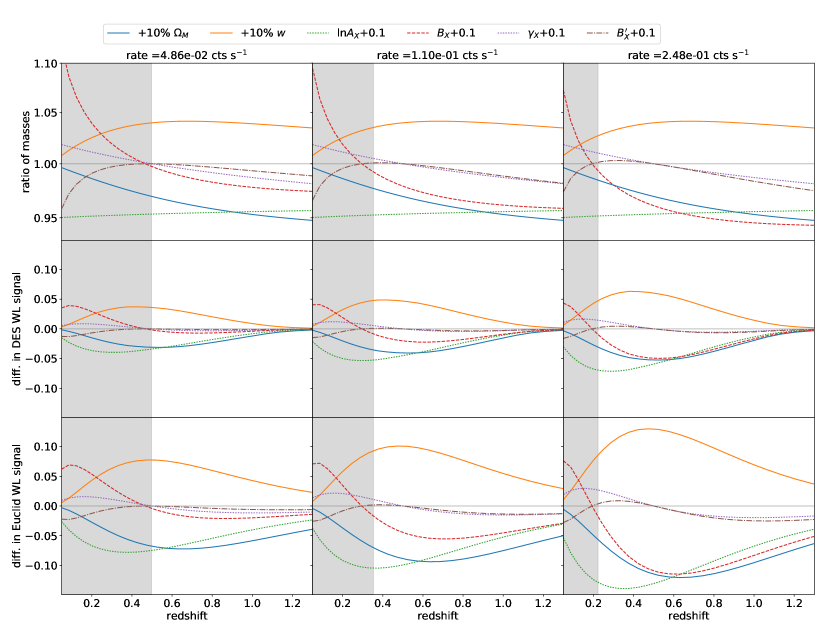
Figure 9: Sensitivity of different mass observables to the parameters considered in this work. On the x-axis, we plot the redshift and each column represents a different count rate. The parameters are varied around the input values. The grey area shows the observable range which is excluded by the approximate mass cut. From the top, the first row shows the fractional change in mass. The second and third rows show the difference in tangential shear for a single cluster, weighted by the observational WL uncertainty for a single cluster at that redshift, for DES and Euclid, respectively. We also see that both for the halo masses and for the shear signal, $\Omega_{\text{M}}$ and $w$ lead to changes comparable to the change in amplitude $\ln A_{\text{X}}$ and $\gamma_{\text{X}}$. We conclude that these parameters must be degenerate with each other.

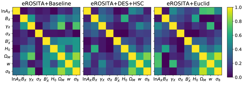
Figure 10: Absolute values of the correlation matrices of the posterior samples in the $w$CDM model, for number count (eROSITA+Baseline), number counts with DES+HSC WL information (eROSITA+DES+HSC) and number counts with Euclid WL information (eROSITA+Euclid). Noticeably, we find that the initial correlations between the pairs $(\Omega_{\text{M}},\sigma_{8})$ and $(B_{\text{X}},\gamma_{\text{X}})$ (in eROSITA+Baseline) is gradually broken by the addition of better mass information (eROSITA+DES+HSC and eROSITA+Euclid). However, the better the mass information, the clearer the inherent correlations between $w$, $\Omega_{\text{M}}$, $A_{\text{X}}$ and $\gamma_{\text{X}}$. They indicate the degeneracies among these parameters stemming from the cosmology dependence of the rate mass mapping, as discussed in Section 5.2.

To investigate in more detail how our observables– i.e. the number counts of clusters as a function of rate and redshift together with the WL mass calibration information– depend on the model parameters, we perform the following experiment: we vary the model parameters one by one and examine how the number counts, the masses and the WL signals change. The results of this test are shown in Figs. 8 and 9. At three different fixed rates (increasing from left to right in the three columns), we investigate the sensitivity as a function of redshift with respect to the input parameter of the likelihood of the number counts (Fig. 8), as well as the masses, and the WL signals (Fig. 9). We grey out the part of rate–redshift space that is rejected due to our mass cut.

5.2.1 Number counts

Fig. 8 shows the sensitivity of the number counts with respect to shifts in the input parameters. We decide here to plot the difference in log likelihood between the fiducial number counts $N_{\text{fid}}$ and the number counts $\tilde{N}$ if one parameter is varied. The difference in log likelihood in each bin reads

$$\delta\ln L=N_{\text{fid}}\ln\left(\frac{N_{\text{fid}}}{\tilde{N}}\right)-N_{\text{fid}}+\tilde{N},$$ (21)

which can be simply obtained by taking the Poisson log likelihoods in that bin. We find that the number counts are most sensitive to the parameters $\Omega_{\text{M}}$ and $A_{\text{S}}$. The sensitivity to the parameters $w$, $A_{\text{X}}$, $B_{\text{X}}$, and $\gamma_{\text{X}}$ is much lower. This is reflected also in our results for the parameter uncertainties (Tables 3 and 4). The number counts do put tighter constraints on $\Omega_{M}$ and $\sigma_{8}$, than on $w$, consistent with results from the first forecast studies for large scale cluster surveys (Haiman et al., 2001; Holder et al., 2001).

For comparison we also plot the total number of objects $N_{\text{fid}}$ (dashed line), on a scale proportional to the difference in log likelihood. We can readily see that the difference in log likelihood is not simply proportional to the number of objects: the rarer, higher redshift, and consequently, at fixed rate, higher mass objects contribute more log likelihood per cluster than the lower redshift, lower mass systems. This trend is especially true for the constraints on $\Omega_{M}$ and $\sigma_{8}$ ($A_{\mathrm{S}}$), as noted in previous studies of cluster number counts (Haiman et al., 2001; Majumdar & Mohr, 2004). The sensitivity to 10% shifts in $w$ and $A_{\mathrm{X}}$ are comparable. The more similar the shapes of the sensitivity curves for two parameters, the stronger the parameter degeneracy one could expect between those parameters.

5.2.2 Masses and WL observables

The first row of Fig. 9 shows how much the masses are impacted by changes in input parameters. To this end, we plot the ratio between the input mass and the mass determined at the shifted parameters. In the range of interest for our study, the white area, we find that all parameters (except for $A_{\text{S}}$, of course, which we do not include in this figure) have a comparably large impact on the masses. Most remarkably, both shifts in $\Omega_{\text{M}}$ and $w$ change the masses associated to a given rate and redshift. This is because the rate mass relation has a strong distance dependence and also some critical density dependence. Both $\Omega_{\text{M}}$ and $w$ alter the redshift dependence of distances and critical densities.

More precisely, the shift to more positive $w$ leads to a shift to higher masses, which mirrors the effect of changing the amplitude of the scaling relation $\ln A_{\text{X}}$ and the redshift slope $\gamma_{\text{X}}$. Similarly, the redshift dependent mass shift induced by $\Omega_{\text{M}}$ could be compensated by a shift in the redshift slope $\gamma_{\text{X}}$ and $\ln A_{\text{X}}$. We therefore conclude that within the context of the masses corresponding to a fixed eROSITA count rate, the parameters $w$ and $\Omega_{\text{M}}$ are degenerate with a combinations of $\ln A_{\text{X}}$ and $\gamma_{\text{X}}$. This degeneracy impacts the predicted halo masses. The mass slope parameter $B_{\text{X}}$, however, seems to impact the masses in a distinctively different way, leading to no obvious parameter degeneracy. The same can be said for its redshift trend $B_{\text{X}}^{\prime}$.

In our main experiment, we do not consider perfect halo masses, but WL signal. Therefore, we explore also the sensitivity of the WL signal for a single cluster to the input parameters. For the sake of simplicity, we do not consider the entire profile, but just assume one large radial bin spanning the fixed metric range corresponding to 0.25 – 5.0 Mpc in our fiducial cosmology. Given the constant metric size of the area considered, the WL measurement uncertainty for a single cluster due to shape noise can be computed by considering the background source density as a function of cluster redshift $n_{\epsilon}(z_{\text{cl}})=n_{\epsilon}(z_{\text{s}}>z_{\text{cl}}+0.1)$. In addition, the mapping from halo mass to tangential shear is non-linear and cosmology dependent. Consequently, the shear signal associated with a given rate and redshift is expected to have strong dependencies on cosmological parameters and, through the mass, also on the scaling relation parameters.

We visualize these effects in the second and third rows of Fig. 9 by plotting the difference between the WL signal for a single cluster in the fiducial model and the shifted model, divided by the expected magnitude of the shape noise for a single cluster. Indeed, one can readily see how the sensitivity per cluster of DES WL (second row) is generally lower, but also decreases more quickly with redshift than the sensitivity of Euclid WL (third row). This is due to the larger Euclid source galaxy sample and its extension to higher redshift as compared to DES. The trends we discuss above for the difference in halo mass do apply also to the sensitivity of the WL signal as a function of redshift.

We find the same degeneracies in the covariance matrices of our posterior samples in the $\nu$-$w$CDM model for the three cases of eROSITA+baseline, eROSITA+DES+HSC, and eROSITA+Euclid, shown in Fig. 10. In the case of number counts alone, we find a strong correlation between the pairs $(\Omega_{\text{M}},\sigma_{8})$ and $(B_{\text{X}},\gamma_{\text{X}})$. The latter degeneracy is strongly reduced by the addition of WL mass information, and is not present in the case of Euclid WL calibration. This is due to the fact that WL is quite sensitive to $B_{\text{X}}$. This is in line with improvements of both the $(\Omega_{\text{M}},\sigma_{8})$ and $B_{\text{X}}$ constraints when adding WL mass information. However, when $w$ is free to vary, the degeneracies between $w$, $\ln A_{\text{X}}$ and $\gamma_{\text{X}}$ lead to stronger correlations between these parameters for better mass information. They are most pronounced in the case of number counts with Euclid WL mass calibration.

5.3 Comparison to previous work

Finally, we compare our results to the constraints of recent and future experiments, with the intention of exploring how competitive eROSITA will be.

5.3.1 Current probes

The most up to date number counts analysis of an X-ray selected sample with WL mass calibration has been presented by Mantz et al. (2015, called Weighing the Giants, hereafter WtG). It consists of 224 clusters, 51 of which have a WL mass measurement, and 91 of which have ICM mass measurements. The analysis method is similar to the one described in this paper, with the exception that we did not consider cosmological constraints from the measurement of the ICM mass fraction. In the $w$CDM model (i.e. fixing the neutrino mass), when considering only X- ray and WL data, the uncertainties on $\Omega_{\text{M}}$, $\sigma_{8}$ and $w$ are 0.036, 0.031 and 0.15, respectively. The direct comparison to our work is made difficult by the addition of the distance sensitive gas fraction measurements, which by themselves constrain $\delta\Omega_{\text{M}}=0.04$ and $\delta w=0.26$ (Mantz et al., 2014). This measure clearly dominates the error budget on $\Omega_{\text{M}}$ and provides valuable distance information. Nevertheless, eROSITA cluster cosmology is evenly matched with WtG when considering just the number counts. It will outperform the constraining power of WtG when calibrated with DES+HSC WL information. In the case of LSST WL calibration, we project that the uncertainties on $\Omega_{\text{M}}$, $\sigma_{8}$ and $w$ are smaller by factors $2.6$, $3.1$ and $2.1$, respectively. These projections ignore distance information from the eROSITA clusters and AGN, which would further improve the constraints.

Another recent cluster cosmology study has been presented by de Haan et al. (2016). Therein, the cosmological constraints from 377 Sunyaev-Zeldovich selected clusters detected by the South Pole Telescope (hereafter SPT) above redshift $>0.25$ are determined. From the number counts alone, the dark energy equation of state parameter is constrained to a precision of $\delta w=0.31$, which is a factor $3.1$ worse than our prediction for the number counts from eROSITA alone. Furthermore, de Haan et al. (2016) find $\delta\Omega_{\text{M}}=0.042$ and $\delta\sigma_{8}=0.039$, while keeping the summed neutrino mass fixed at its minimal value. By comparison, in the baseline configuration eROSITA will improve the constrain on $\Omega_{\text{M}}$ and $\sigma_{8}$ by a factor $1.5$ and $1.2$, however while marginalizing over the summed neutrino mass. Also note that the priors used for the de Haan et al. (2016) analysis encode the mass uncertainty over which Bulbul et al. (2019) marginalized when deriving the uncertainties on the X-ray scaling relation parameters we employ as our eROSITA+Baseline.

When the SPT number counts are combined with the CMB constraints from Planck, de Haan et al. (2016) report constraints on $\sigma_{8}$ and $w$ of $0.045$ and $0.17$ respectively. We find that eROSITA number counts alone, in combination with Planck, will do better by a factor $2.8$ on $\sigma_{8}$ and a factor $2.0$ on the equation of state parameter $w$, while additionally marginalizing over the summed neutrino mass. These numbers improve even more, if we consider the WL mass calibration by DES+HSC, Euclid and LSST.

Comparing our forecasts on the improvement of the upper limit on the summed neutrino mass to previous results from the combination of Planck CMB measurements with either SPT cluster number counts or WtG is complicated by several factors. First, we considere the full mission results for Planck (Planck Collaboration et al., 2016a), while SPT (de Haan et al., 2016) used the half mission data (Planck Collaboration et al., 2014) in addition to BAO data, and WtG (Mantz et al., 2015) additionally added ground based CMB measurements and supernova data. SPT reports the measurement $\sum m_{\nu}=0.14\pm 0.08$ eV, which is impacted to some degree by the statistically insignificant shift between their constraint and the CMB constraints in the $(\Omega_{\text{M}},\sigma_{8})$ plane. Comparison to this result is complicated by our choice to use the minimal neutrino mass as input value. On the other hand, WtG reports $\sum m_{\nu}\leq 0.22$ at 95% confidence, which is comparable with our result from eROSITA number counts, DES+HSC WL, Planck CMB and DESI BAO.

The latest cosmological constraints from measurements of the Large Scale Structure (LSS) of the Universe were presented by the DES Collaboration et al. (2017) for the first year of observations (Y1), where the joint constraints from the cosmic shear and photometric galaxy angular auto- and crosscorrelation functions are derived. In the $\nu$-$w$CDM model, the uncertainties on $\Omega_{\text{M}}$, $\sigma_{8}$ and $w$ are 0.036, 0.028 and 0.21, respectively. This is better than the constraints from eROSITA number counts alone, except for the dark energy equation of state parameter, which will be constrained better by eROSITA. However, utilizing DES+HSC to calibrate the cluster masses, we forecast that eROSITA will outperform the DES-Y1 analysis. In combination with Planck CMB data, DES-Y1 puts a 95% upper limit of 0.62 eV on the sum of the neutrino masses, whereas we forecast an upper limit of 0.424 (0.401) when combining eROSITA number counts (and DES+HSC WL calibration) with Planck data. Considering that our DES WL analysis assumes year 5 data, it will be interesting to see whether the DES Y5 LSS measurements or eROSITA with DES WL calibration will provide the tighter cosmological constraints.

As can be seen from Table 3, eROSITA will clearly outperform Planck CMB measurements on several cosmological parameters. In the $\nu$-$\Lambda$CDM model, eROSITA with WL mass information will outperform Planck on the parameters $\Omega_{\text{M}}$ and $\sigma_{8}$, and in the $\nu$-$w$CDM eROSITA with WL case will also outperform Planck on the equation of state parameter $w$. However, for constraints on the sum of the neutrino mass, Planck alone offers much more than eROSITA alone. Given, however, that eROSITA and Planck extract their constraints at low redshift and high redshift, respectively, the true benefit of these two experiments lies in assessing the mutual consistency and thereby probing whether our evolutionary model of the Universe is correct. If this is the case, their joint constraints will tightly constrain the cosmological model, and provide improved constraints on the sum of neutrino masses.

5.3.2 Previous forecasts for eROSITA

This work elaborates further on the forecast of the eROSITA cosmological constraints first presented in Merloni et al. (2012), and subsequently discussed in more detail in P18. The direct comparison to the latter is complicated by several diverging assumptions, including that we only consider the German half of the sky. Perhaps the most significant difference is their approach of using Fisher matrix estimation and modeling mass calibration as simply being independent priors on the various scaling relation parameters, whereas we have developed a working prototype for the eROSITA cosmology pipeline and used it to analyze a mock sample with shear profiles in a self-consistent manner.

Other differences include their use of different input scaling relations from older work at lower redshift and different fiducial cosmological parameters. P18 includes constraints from the angular clustering of eROSITA clusters, although these constraints are subdominant in comparison to counts except for parameters associated with non-Gaussianity in the initial density fluctuations (see Pillepich et al., 2012). In our analysis, we marginalize over the sum of the neutrino mass as well as relatively weak priors on $\omega_{\mathrm{b}}$ and $n_{\mathrm{S}}$.

Following what P18 call the pessimistic case with an approximate limiting mass of $5\times 10^{13}M_{\sun}h^{-1}$, they predict 89 k clusters, which is in good agreement with our forecast of 43 k clusters when including clusters down to masses of $5\times 10^{13}M_{\sun}$. Under the assumption of a 0.1 % amplitude prior, 14 % mass slope prior and 42 % redshift slope prior, they forecast a constraint of $0.017$, $0.014$ and $0.059$ on $\sigma_{8}$, $\Omega_{\text{M}}$ and $w$, respectively. P18 also consider an optimistic case, in which clusters down to masses of $1\times 10^{13}M_{\sun}h^{-1}$ are used under the assumption of 4 times better priors on the scaling relation parameters. For this case, the constraints on $\sigma_{8}$, $\Omega_{\text{M}}$ and $w$ are $0.011$, $0.008$ and $0.037$, respectively.

A quantitative comparison to our work is complicated by the fact that we find a constraint on the amplitude of the scaling relation (through direct modeling of the WL calibration from Euclid or LSST) that is worse than their pessimistic case, but our constraint on the mass and redshift trends is better than their optimistic case. Consistently, we predict tighter constraints of $\sigma_{8}$ and $\Omega_{\text{M}}$, which are sensitive to the mass and redshift trends of the scaling relation, while we predict lower precision on $w$, which we demonstrate to be degenerate with the amplitude of the scaling relation through the amplitude distance degeneracy. Important here is the realization that the observed shear profiles map into cluster mass constraints in a distance dependent fashion (this is true for all direct mass constraints; Majumdar & Mohr, 2003). It is not straightforward to capture this crucial subtlety by simply adopting priors on observable mass scaling relation parameters.

5.3.3 Euclid cosmological forecasts

The Euclid survey will not only provide shear catalogs to calibrate the masses of clusters, but will also allow the direct detection of galaxy clusters via their red galaxies (Sartoris et al., 2016), and the measurement of the auto- and cross-correlation of red galaxies and cosmic shear (Giannantonio et al., 2012). For the optically selected Euclid cluster sample, Sartoris et al. (2016) forecast $2\times 10^{6}$ galaxy clusters with limiting mass of $7\times 10^{13}M_{\sun}$ up to redshift $z=2$, yielding constraints on $\Omega_{\text{M}}$, $\sigma_{8}$, and $w$ of $0.0019$ ($0.0011$), $0.0032$ ($0.0014$), and $0.037$ ($0.034$), respectively, when assuming no knowledge on the scaling relation parameter (perfect knowledge of the scaling relation parameters). Under these assumptions, the number counts and the angular clustering of Euclid selected clusters would outperform eROSITA cluster cosmology. Nevertheless, cross comparisons between the X-ray based eROSITA selection and the optically based Euclid cluster selection will provide chances to validate the resulting cluster samples.

Giannantonio et al. (2012) forecast that the auto- and cross-correlations between red galaxies and cosmic shear in the Euclid survey will provide constraints on $\Omega_{\text{M}}$, $\sigma_{8}$, and $w$ of $0.005$, $0.033$ and $0.050$, respectively. Such a precision on $\sigma_{8}$ would be achieved by the baseline eROSITA+Euclid analysis, too. However, to achieve similar precisions in $\Omega_{\text{M}}$ and $w$, it would be necessary to consider eROSITA detected clusters down to masses of $5\times 10^{13}\text{M}_{\sun}$.

6 Conclusions

In this work, we study the impact of WL mass calibration on the cosmological constraints from an eROSITA cluster cosmology analysis. To this end, we create a mock eROSITA catalog of galaxy clusters. We assign luminosities and ICM temperatures to each cluster using the latest measurements of the X-ray scaling relations over the relevant redshift range (Bulbul et al., 2019). Considering the eROSITA ARF, we then compute the eROSITA count rate for all clusters in this sample. We apply a selection on the eROSITA count rate, corresponding to a $\sim 6\sigma$ detection limit given current background estimates, to define a sample for a cosmological forecast. This detection limit ensures both high likelihood of existence and angular extent, and – through raising the detection threshold at low redshift – also excludes low mass objects at low redshift. We assume all cluster redshifts are measured photometrically using red sequence galaxies (see discussion in, e.g. Klein et al., 2018; Klein et al., 2019). We forecast that in the 14,892 deg² of the low Galactic extinction sky accessible to the eROSITA-DE collaboration, when raising the detection threshold at low redshift to exclude clusters with $M_{500\text{c}}\lessapprox 2\times 10^{14}\text{M}_{\sun}$, we predict that eROSITA will detect 13k clusters. This baseline cosmology sample has a median mass of $\bar{M}_{500\text{c}}=2.5\times 10^{14}\text{M}_{\sun}$ and a median redshift of $\bar{z}=0.51$. For the case where we adjust the low redshift detection threshold to exclude clusters with $M_{500\text{c}}\lessapprox 5\times 10^{13}\text{M}_{\sun}$, we predict 43k clusters. This sample has a median mass $\bar{M}_{500\text{c}}=1.4\times 10^{14}\text{M}_{\sun}$, and a median redshift $\bar{z}=0.31$. Both samples extend to high redshift with $\sim 400$ clusters at $z>1$.

We then analyze these mock samples using a prototype of the eROSITA cluster cosmology code that is an extension of the code initially developed for SPT cluster cosmology analyses (Bocquet et al., 2015; de Haan et al., 2016; Bocquet et al., 2018). This codes employs a Bayesian framework for simultaneously evaluating the likelihoods of cosmological and scaling relation parameters given the distribution of clusters in observable and redshift together with any direct mass measurement information. The scaling relation between the selection observable (eROSITA count rate) and the mass and redshift is parametrized as a power law with log-normal intrinsic scatter. Final parameter constraints are marginalized over the uncertainties (systematic and statistical) in the parameters of the mass– observable scaling relation.

We first estimate the optimal level of mass calibration necessary for the number counts of eROSITA clusters to mainly inform the constraints on the cosmological parameters. This requires a calibration of the amplitude of the mass observable relation at 4.2%, the mass trend of the scaling relation at 2.4%, and the redshift trend at 5.3%. These numbers are derived using current knowledge of the scatter around the mass luminosity relation. Furthermore, we determine that the mass trend of the rate mass relation has to be allowed to vary with redshift to enable the recovery of unbiased cosmological results.

We then examine cosmological constraints in three different cluster mass calibration contexts: (1) using "baseline" constraints existing today that are taken from the recent SPT analysis of the X-ray luminosity and temperature mass relations (Bulbul et al., 2019), (2) using WL information from the DES+HSC survey and (3) using WL information from the future Euclid and LSST survey. For the subset of the two catalogs that overlap the DES, HSC, Euclid or LSST survey footprints, we produce tangential shear profiles with appropriate characteristics for these surveys. We also estimate the level of systematic mass uncertainties in the WL masses that would result from the data quality of these two surveys and from theoretical uncertainties in the impact of mis-centering and mis-fitting the shear profiles. We adopt mass uncertainties of 5.1%, 1.3% and 1.5% for DES+HSC, Euclid, and LSST, respectively. These levels of systematic mass uncertainty will require that our understanding of the theoretical mass bias from simulations be improved by factors of 2 and 5 for DES+HSC and Euclid/LSST, respectively, in comparison to current work (Dietrich et al., 2019). We note that achieving these improvements will require a significant investment of effort.

Throughout this work, we allow the summed neutrino mass to vary. All results are thus marginalized over the summed neutrino mass. In the $\nu$-$w$CDM model, we forecast that eROSITA number counts will constrain the density of matter in the Universe $\Omega_{\text{M}}$ to 0.032, the amplitude of fluctuation $\sigma_{8}$ to 0.052, and the equation of state parameter of the dark energy $w$ to 0.101. Calibrating the masses of eROSITA clusters with DES+HSC (Euclid; LSST) WL will reduce these uncertainties to 0.023 (0.016; 0.014), 0.017 (0.012; 0.010), and 0.085 (0.074; 0.071), respectively. We also find that eROSITA clusters alone will not provide appreciable constraints on the sum of the neutrino masses.

eROSITA number counts will be able to break several degeneracies in current CMB constraints, especially on late time parameters such as $\Omega_{\text{M}}$, $\sigma_{8}$ and $w$. In combination with Planck constraints from the measurement of the angular auto- and crosscorrelation functions of CMB temperature and polarization anisotropies, we determine that eROSITA will constrain these parameters to 0.019, 0.032 and 0.087 when adopting "baseline" priors on the scaling relation parameters. These uncertainties shrink to 0.018 (0.014; 0.013), 0.019 (0.010; 0.009) and 0.085 (0.074; 0.069) when calibrating the masses with DES+HSC (Euclid; LSST) WL information.

When considering the $\nu$-$\Lambda$CDM model, the upper limit on the neutrino mass of 0.514 eV from CMB alone can be improved to a constraint of 0.425 eV when utilizing number counts with the "baseline" priors, 0.404 eV when also considering DES WL calibration, and to 0.291 eV when calibrating with Euclid WL, and 0.285 eV when calibrating with LSST WL.

We find that the constraining power of eROSITA cluster cosmology, even when calibrated with high quality shear profiles, is limited by a degeneracy between the scaling relation parameters and the cosmological distance to the clusters. This degeneracy arises, because the luminosity distance is necessary to transform observed count rates into luminosities, whose absolute and redshift dependent scaling with mass needs to be fitted simultaneously with the cosmological parameters that alter the redshift distance relation. This leads to the assessment that even the Euclid or LSST WL mass calibration will, by itself, not reach what we have defined as optimal levels in the $\nu$-$w$CDM model.

However, we demonstrate that, with the inclusion of BAO measurements that constrain the redshift distance relation, the Euclid or LSST WL dataset can be used to calibrate cluster masses at an optimal level. Considering DESI-like BAO measurements, we project that eROSITA with Euclid WL mass calibration will constrain $\sigma_{8}$ to 0.005 and $w$ to 0.047, while the uncertainty on $\Omega_{\text{M}}$ will be dominated by the BAO measurement.

Furthermore, we investigate the impact of lowering the mass limit to $M_{\text{500c}}\goa 5\times 10^{13}\text{M}_{\sun}$. Given the larger number of low mass clusters or groups, the eROSITA counts with Euclid WL can optimistically be used to determine $\Omega_{\text{M}}$ to 0.009, $\sigma_{8}$ to 0.007, and $w$ to 0.056, if these low mass systems are simple extrapolations of the high mass systems. The expected additional complexity of these low mass systems would have to be modeled, and this additional modeling would likely weaken the cosmological constraints.

In summary, WL mass calibration from DES+HSC, Euclid, and LSST will significantly improve cosmological constraints from eROSITA cluster number counts, enabling a precise and independent cross-check of constraints from other measurements. The constraining power on $w$ suffers from an inherent degeneracy between the distance redshift relation and the scaling relation between the X-ray observable, mass and redshift. This degeneracy can be lifted by inclusion of other cosmological measurements, such as BAO or CMB measurements. In turn eROSITA cluster cosmology can break degeneracies in these other observations, underscoring the synergies between different cosmological experiments.

Appendix A Comments on selection

Figure 11: Estimated significance of detection (left panel) and significance of extent (right panel) as functions of redshift for a cluster with 15, 40, and 100 photons, and clusters of halo mass $M_{500c}=5\times 10^{13}$ M_☉, and $2\times 10^{14}$ M_☉ for median exposure time and background brightness. We find that 40 (15, 100) photon counts corresponds, at least, to a 8$\sigma$ (3$\sigma$, >10$\sigma$) detection and a $3.5\sigma$ (2 $\sigma$, 9$\sigma$) significance of extent, rather independently of the cluster redshift.

In this work, we assume two selection criteria for our X-ray cluster sample:

• a cut in measured number of photons $\hat{n}_{\gamma}>40$ cts, which for the median eROSITA field with an exposure time of $1.6$ ks translates into a measured rate cut $\hat{\eta}>2.5\times 10^{-2}$ cts s^-1,

• a cut in the observed mass

  $$\begin{split}M_{\text{obs}}=&M_{\text{0}}\,e^{-\frac{\ln A_{X}}{B(z)}}\left(\frac{\hat{\eta}}{\eta_{0}}\right)^{\frac{1}{B(z)}}\left(\frac{E(z)}{E_{0}}\right)^{-\frac{2}{B(z)}}\left(\frac{D_{\text{L}}(z)}{D_{\text{L}}(z_{0})}\right)^{\frac{2}{B(z)}}\\ &\left(\frac{1+z}{1+z_{0}}\right)^{-\frac{\gamma(z)}{B(z)}},\end{split}$$ (22)

  which is derived from the rate-mass scaling relation equation (7). It is evaluated for the fiducial cosmology and the fiducial scaling relation parameters derived in Appendix B. The cut $M_{\text{obs}}>2\times 10^{14}\text{M}_{\sun}$, or $M_{\text{obs}}>5\times 10^{13}\text{M}_{\sun}$ is thus provided by a function of redshift, which is independent of cosmology and of the scaling relation parameters, and leads to the above mentioned cuts $M_{500\text{c}}\goa 2\times 10^{14}\text{M}_{\sun}$ or $M_{500\text{c}}\goa 5\times 10^{13}\text{M}_{\sun}$. The low mass cut is thus implemented as a redshift dependent cut in observables (as for instance also in Vikhlinin et al., 2009a; Pillepich et al., 2012).

The cut at $\hat{n}_{\gamma}>40$ cts is justified by the following considerations on X-ray cluster detection. Detection of galaxy clusters hinges on the assumption that galaxy clusters are extended sources in the extragalactic X-ray sky, as discussed, for instance, by Vikhlinin et al. (1998) in the case of the ROSAT PSPC, Pacaud et al. (2006) in the case of XMM-Newton, and Clerc et al. (2018) in the context of eROSITA. For this reason, their extraction is usually divided into two steps: first all X-ray sources are identified, then, among the identified source, those who are extended are selected. As outlined in Clerc et al. (2018), eROSITA will follow a similar procedure.

Following Pacaud et al. (2006), consider an X-ray image with a number of photons in each pixel $i$ given by $\hat{n}_{i}$, and define the following three likelihoods:

• the likelihood that the image is simply background with background brightness $\mu_{\text{bkg}}$, which reads

  $$\ln\mathcal{L_{\text{bkg}}}=\sum_{i}\hat{n}_{i}\ln(\mu_{\text{bkg}}\,\text{A}_{i})-\mu_{\text{bkg}}\,\text{A}_{i},$$ (23)

  where $\text{A}_{i}$ is the area of each pixel $i$;

• the likelihood of being a point source centered in $\mathbf{x}_{\text{ps}}$ with total number of photons $n_{\text{ps}}$, given by

  $$\begin{split}\ln\mathcal{L_{\text{ps}}}=&\sum_{i}\hat{n}_{i}\ln(n_{\text{ps}}\text{PFS}(\mathbf{x_{\text{ps}}})_{i}+\mu_{\text{bkg}}\,\text{A}_{i})\\ &-n_{\text{ps}}\text{PFS}(\mathbf{x_{\text{ps}}})_{i}-\mu_{\text{bkg}}\,\text{A}_{i}\end{split}$$ (24)

  where $\text{PFS}(\mathbf{x})_{i}$ is the value in the pixel $i$ of the average survey point spread function (PSF) centered in $\mathbf{x}$;

• the likelihood of being a cluster with total number of photons $n_{\gamma}$, modeled as the convolution of a $\beta$-model (Cavaliere & Fusco-Femiano, 1976) with the PSF, which, for a cluster position $\mathbf{x}$ and cluster core radius $\theta_{c}$, reads

  $$\begin{split}\ln\mathcal{L_{\text{cl}}}=&\sum_{i}\hat{n}_{i}\ln(n_{\gamma}S(\mathbf{x};\theta_{c})_{i}+\mu_{\text{bkg}}\,\text{A}_{i})\\ &-n_{\gamma}S(\mathbf{x};\theta_{c})_{i}-\mu_{\text{bkg}}\,\text{A}_{i},\end{split}$$ (25)

  where $S(\mathbf{x};\theta_{c})_{i}$ stands for the value of the PSF convolved beta-profile with center $\mathbf{x}$ and core radius $\theta_{c}$.

For the median eROSITA field, we expect $\mu_{\text{bkg}}=3.6$ cts arcmin^-2 (Clerc et al., 2018). To estimate the approximate significances of clusters with $n_{\gamma}=(15,40,100)$ at different redshifts, we use the rate- mass relation derived in this work (c.f. Section 3.1). Furthermore, we assume that the core radius is given by $\theta_{c}=0.2\theta_{500c}$, where $\theta_{500c}$ is the angular extent of the radius inclosing an over density 500 times the critical density of the Universe. We take the PSF to be a gaussian with half energy width of $24$ arcsec. Assuming $\beta=2/3$, we create an X-ray 10-by-10 arcmin image of the expected number of photons $\hat{n}$, by computing $\hat{n}_{i}=n_{\gamma}S(\mathbf{x};\theta_{c})_{i}+\mu_{\text{bkg}}\,\text{A}_{i}$. We intentionally do not draw a Poisson realization of the model, in order to capture the mean behavior of the extraction procedure.

On this image, the three likelihoods are then maximized by varying ($n_{\text{ps}}$, $\mathbf{x}_{\text{ps}}$), and ($n_{\gamma}$, $\theta_{c}$, $\mathbf{x}$), respectively. We shall denote the maximum likelihood $\ln\hat{\mathcal{L}}_{\alpha}$ for $\alpha\in$ (bkg, ps, cl). To create an analogy to the SZE case, which can be interpreted as "sigmas", both for detection $\xi_{\text{det}}=\sqrt{2(\ln\hat{\mathcal{L}}_{\text{cl}}-\ln\hat{\mathcal{L}}_{\text{bkg}})}$, and for extent $\xi_{\text{ext}}=\sqrt{2(\ln\hat{\mathcal{L}}_{\text{cl}}-\ln\hat{\mathcal{L}}_{\text{ps}})}$. Note that for well detected point sources, the best fit core radius $\theta_{c}\approx 0$, such that $\ln\hat{\mathcal{L}}_{\text{cl}}\approx\ln\hat{\mathcal{L}}_{\text{ps}}$ and $\xi_{\text{ext}}\approx 0$, while $\xi_{\text{det}}\gg 0$. In contrast, for well detected extended sources, $\xi_{\text{det}}\gg 0$ and $\xi_{\text{ext}}\gg 0$. For practical purposes, the region in which the likelihood is maximized is often pre-selected.

We repeat this exercise for different redshifts. The results are shown in Fig. 11. We find that a source with 40 (15, 100) photons will be detected, at least, at 8$\sigma$ (3$\sigma$, 10$\sigma$) for redshifts above 0.5. Furthermore, we determine that these clusters will have a significance of extent of 3.5$\sigma$ (2$\sigma$, 9$\sigma$). The significance of extension at, e.g., 15 or 40 photons, is rather low. Extent acts as a secondary selection on a sample which contains approximately 10% clusters and 90% point sources. Considering that 3.5$\sigma$ (2$\sigma$) corresponds to a p-value of $2.3\times 10^{-4}$ ($2.3\times 10^{-2}$), the extent cut would create a cluster sample with an approximate contamination of 0.2% (17%) by point sources after the X-ray selection. With the optical followup of a tool like MCMF, any X-ray cluster candidate without an associated overdensity of red galaxies can be easily removed from the sample (Klein et al., 2018; Klein et al., 2019).

Fig. 11 also shows the redshift evolution of the significances for a cluster of fixed mass. The characterization of this evolution, especially its dependence on distance both through the flux and the angular extent, might be worth further investigation, as its knowledge would allow us to use the significance as a the primary X-ray observable. Such a study is currently limited by the somewhat simplistic assumption that the core radius is a multiple of the virial radius $\theta_{500c}$. Furthermore, a study of the measurement uncertainty on the significance would be necessary.

Appendix B Comments on the count rate to mass relation

To obtain unbiased cosmological results, the parametric form of the scaling relation needs to provide accurate mass predictions over the mass and redshift range of interest for the sample considered. This is necessary, as systematic biases in mass lead to a systematic misestimation of the abundance of clusters in a given observable redshift range. These misestimations of cluster abundance will then be compensated by shifts in the cosmological parameters, which would generically lead to systematic biases in the best fitting cosmological parameters. Therefore, it is of paramount importance to utilize a parametric form for the scaling relation that has adequate freedom to describe the sample being modeled.

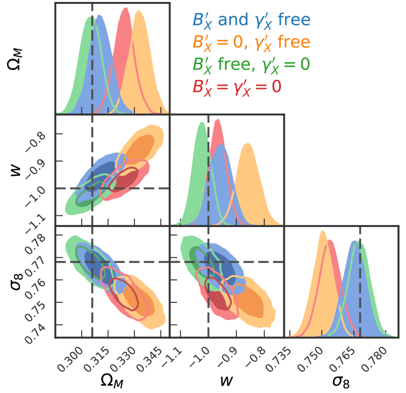
Figure 12: Cosmological constraints derived from a ten times larger sample in four cases: free $B_{\text{X}}^{\prime}$ and $\gamma_{\text{X}}^{\prime}$, free $B_{\text{X}}^{\prime}$ and $\gamma_{\text{X}}^{\prime}=0$, $B_{\text{X}}^{\prime}=0$ and free $\gamma_{\text{X}}^{\prime}$, and $B_{\text{X}}^{\prime}=\gamma_{\text{X}}^{\prime}=0$. Noticeable shift in the inferred cosmological parameters occur once $B_{\text{X}}^{\prime}=0$, whereas the case of free $B_{\text{X}}^{\prime}$ and $\gamma_{\text{X}}^{\prime}=0$ is very similar to the maximal case.

B.1 Scaling relation form

It is worth noting that even though the observed X-ray luminosity to mass and temperature to mass relations show no evidence supporting a redshift dependent mass trend or a changing power law in the redshift trend (Bulbul et al., 2019), the mass and redshift dependences of the eROSITA count rate to flux conversion could introduce these additional trends into the count rate to mass scaling relation (equation 7). Here we explore whether these additional freedoms are needed in the forecasts we perform.

The ratio between the eROSITA count rate of a cluster and its rest frame 0.5-2 keV flux, which we shall call $K=\eta/f_{\text{X}}$, parameterizes the response of the eROSITA cameras to a specific spectral form and the k-correction necessary to account for the transformation from rest frame 0.5-2 keV to the observed frame. As such, one would expect it to be both redshift and temperature dependent. The rate can be written as

$$\eta=K\,f_{\text{X}}=K\,\frac{L_{X}}{4\pi d_{\mathrm{L}}^{2}(z)}.$$ (26)

Thus, conceptually, the rate mass redshift scaling equals the luminosity mass redshift scaling, with the addition of the luminosity distance dependence and the mass and redshift trends of the flux to rate conversion.

$K$ has a noticeable but weak redshift dependence, and this redshift dependence is different for clusters of different temperature. The redshift dependence leads to the difference between the redshift trends of the rate and luminosity to mass relations (i.e., parameters $\gamma_{\text{X}}$ and $\gamma_{\text{L}}$), while the temperature dependence of this redshift trend combined with the temperature to mass redshift scaling leads to a non vanishing redshift variation in the mass trend of the rate scaling relation.

The baseline scaling relation for our analysis (equation 7) already has a redshift dependent mass trend parameter $B_{\text{X}}^{\prime}$ (equation 8). Here we introduce a generalization to equation (7) by allowing a redshift trend $\gamma^{\prime}_{\text{X}}$ in the redshift slope

$$\gamma(z)=\gamma_{\text{X}}+\gamma_{\text{X}}^{\prime}\ln\left(\frac{1+z}{1+z_{0}}\right),$$ (27)

which allows for the power law index in redshift to change with redshift.

We examine the importance of this additional redshift dependence by fitting the scaling relation described by the full parameter set $(\ln A_{\text{X}},B_{\text{X}},\gamma_{\text{X}},\sigma_{\text{X}},B_{\text{X}}^{\prime},\gamma_{\text{X}}^{\prime})$ using both true masses and Euclid WL mass constraints and allowing the parameter values to vary within large priors. Such an analysis is straightforward in the controlled regime of a mock catalog analysis where true masses and therefore the underlying form of the scaling known. In analyzing the real eROSITA dataset, one must use direct mass constraints like those from WL or dynamical masses to carry out a goodness of fit test for any proposed scaling relation form (as done in the SPT analyses; Bocquet et al., 2015; de Haan et al., 2016).

We analyze the number counts with perfect and with Euclid WL constraints for the 10 times larger validation mock (cf. Section 3.2.4) using effectively four different mass observable relations. As a baseline we sample both $B_{\text{X}}^{\prime}$ and $\gamma_{\text{X}}^{\prime}$, the two parameters that allow for redshift variation of the mass and redshift trends. We then also consider the cases where either or both of the two extra parameters are set to zero. The resulting constraints on the cosmological parameters of interest are shown in Fig. 12. We find that the run with $\gamma_{\text{X}}^{\prime}=0$ has constraints comparable to the baseline case where both $B_{\text{X}}^{\prime}$ and $\gamma_{\text{X}}^{\prime}$ are free. On the other hand, the run with $B_{\text{X}}^{\prime}=0$ produces biased cosmological parameters. This finding is consistent with the conclusions of Pillepich et al. (2012), who– although not using a rate mass scaling with empirical calibration, noted nonetheless that the effective rate mass scaling they derived had a mass slope which varied with redshift. We thus conclude that the parameter $B_{\text{X}}^{\prime}$ needs to be sampled, while the parameter $\gamma^{\prime}_{\text{X}}$ can be fixed to zero without biasing the cosmological inference at a level that is important, given the statistical uncertainties. In principle this parameter could also be left free to float without any bias implications, but adding more free parameters than needed in the mass observable relation tends to reduce the precision of the constraints on all parameters.

Table 5: Results for the scaling relation parameters when using the perfect halo mass $M_{\text{500c}}$ to calibrate the mass observable relation. These values are used as fiducial values for the scaling relation parameters in the rest of the work.

$\ln A_{\text{X}}$	$B_{\text{X}}$	$\gamma_{\text{X}}$	$\sigma_{X}$	$B^{\prime}_{\text{X}}$
-0.328	1.997	0.446	0.278	0.355

B.2 Fiducial parameter values

To determine the fiducial values for the parameters of the scaling between rate and mass, we sample the mass calibration likelihood with perfect masses. We adopt the form justified in the previous section, where $\gamma^{\prime}_{\text{X}}=0$ (see equation 7). The best fit scaling relation parameters when perfect masses are used are reported in Table 5. They are used as fiducial values in several occasions during this work. The value of $\ln A_{\text{X}}$ can be rescaled arbitrarily by changing the pivot points $\eta_{\text{0}}$, $M_{\text{0}}$ and $z_{\text{0}}$. $B_{\text{X}}$ and $\sigma_{\text{X}}$ take values very similar to the mass slope of the luminosity mass relation $B_{\text{L}}$ and the scatter around that relation $\sigma_{\text{L}}$, respectively. For the values presented in Table 5, we have sampled the mass calibration likelihood for perfect masses discussed in Eq. (10). The value for $\gamma_{\text{X}}$ is larger then the redshift slope of the luminosity–mass scaling. Also, there is a clear preference for redshift evolution of the mass trend.

References

- Anders & Grevesse (1989) Anders E., Grevesse N., 1989, Geochimica Cosmochimica Acta, 53, 197
- Applegate et al. (2014) Applegate D. E., et al., 2014, MNRAS, 439, 48
- Bardeau et al. (2007) Bardeau S., Soucail G., Kneib J.-P., Czoske O., Ebeling H., Hudelot P., Smail I., Smith G. P., 2007, A&A, 470, 449
- Barnes et al. (2017) Barnes D. J., et al., 2017, MNRAS, 471, 1088
- Bartelmann (1996) Bartelmann M., 1996, A&A, 313, 697
- Baxter et al. (2015) Baxter E. J., et al., 2015, ApJ, 806, 247
- Baxter et al. (2018) Baxter E. J., et al., 2018, MNRAS, 476, 2674
- Becker & Kravtsov (2011) Becker M. R., Kravtsov A. V., 2011, ApJ, 740, 25
- Benson et al. (2013) Benson B. A., et al., 2013, ApJ, 763, 147
- Bharadwaj et al. (2014) Bharadwaj V., Reiprich T. H., Schellenberger G., Eckmiller H. J., Mittal R., Israel H., 2014, A&A, 572, A46
- Bleem et al. (2015) Bleem L. E., et al., 2015, ApJS, 216, 27
- Bocquet & Carter (2016) Bocquet S., Carter F. W., 2016, ] 10.21105/joss.00046, 1
- Bocquet et al. (2015) Bocquet S., et al., 2015, ApJ, 799, 214
- Bocquet et al. (2016) Bocquet S., Saro A., Dolag K., Mohr J. J., 2016, MNRAS, 456, 2361
- Bocquet et al. (2018) Bocquet S., et al., 2018, arXiv e-prints,
- Böhringer et al. (2001) Böhringer H., et al., 2001, A&A, 369, 826
- Borm et al. (2014) Borm K., Reiprich T. H., Mohammed I., Lovisari L., 2014, A&A, 567, A65
- Brunner et al. (2018) Brunner H., et al., 2018, in Society of Photo-Optical Instrumentation Engineers (SPIE) Conference Series. p. 106995G, doi:10.1117/12.2315138
- Buchner et al. (2014) Buchner J., et al., 2014, A&A, 564, A125
- Bulbul et al. (2019) Bulbul E., et al., 2019, ApJ, 871, 50
- Capasso et al. (2019) Capasso R., et al., 2019, MNRAS, 482, 1043
- Carlstrom et al. (2011) Carlstrom J., et al., 2011, PASP, 123, 568
- Castorina et al. (2014) Castorina E., Sefusatti E., Sheth R. K., Villaescusa-Navarro F., Viel M., 2014, J. Cosmology Astropart. Phys., 2, 049
- Cavaliere & Fusco-Femiano (1976) Cavaliere A., Fusco-Femiano R., 1976, A&A, 49, 137
- Chiu et al. (2016) Chiu I., et al., 2016, MNRAS, 455, 258
- Chiu et al. (2018) Chiu I., et al., 2018, MNRAS, 478, 3072
- Clerc et al. (2014) Clerc N., et al., 2014, MNRAS, 444, 2723
- Clerc et al. (2018) Clerc N., et al., 2018, A&A, 617, A92
- Cooke et al. (2014) Cooke R. J., Pettini M., Jorgenson R. A., Murphy M. T., Steidel C. C., 2014, ApJ, 781, 31
- Costanzi et al. (2013) Costanzi M., Villaescusa-Navarro F., Viel M., Xia J.-Q., Borgani S., Castorina E., Sefusatti E., 2013, J. Cosmology Astropart. Phys., 12, 012
- DES Collaboration et al. (2017) DES Collaboration et al., 2017, preprint, (arXiv:1708.01530)
- Dark Energy Survey Collaboration et al. (2016) Dark Energy Survey Collaboration et al., 2016, MNRAS, 460, 1270
- Dietrich et al. (2019) Dietrich J. P., et al., 2019, MNRAS, 483, 2871
- Duffy et al. (2008) Duffy A. R., Schaye J., Kay S. T., Dalla Vecchia C., 2008, MNRAS, 390, L64
- Eckmiller et al. (2011) Eckmiller H. J., Hudson D. S., Reiprich T. H., 2011, A&A, 535, A105
- Efstathiou & Bond (1999) Efstathiou G., Bond J. R., 1999, MNRAS, 304, 75
- Evrard et al. (2008) Evrard A. E., et al., 2008, ApJ, 672, 122
- Feroz et al. (2009) Feroz F., Hobson M. P., Bridges M., 2009, MNRAS, 398, 1601
- Font-Ribera et al. (2014) Font-Ribera A., McDonald P., Mostek N., Reid B. A., Seo H.-J., Slosar A., 2014, J. Cosmology Astropart. Phys., 5, 023