A mathematical theory of semantic development in deep neural networks

Abstract

An extensive body of empirical research has revealed remarkable regularities in the acquisition, organization, deployment, and neural representation of human semantic knowledge, thereby raising a fundamental conceptual question: what are the theoretical principles governing the ability of neural networks to acquire, organize, and deploy abstract knowledge by integrating across many individual experiences? We address this question by mathematically analyzing the nonlinear dynamics of learning in deep linear networks. We find exact solutions to this learning dynamics that yield a conceptual explanation for the prevalence of many disparate phenomena in semantic cognition, including the hierarchical differentiation of concepts through rapid developmental transitions, the ubiquity of semantic illusions between such transitions, the emergence of item typicality and category coherence as factors controlling the speed of semantic processing, changing patterns of inductive projection over development, and the conservation of semantic similarity in neural representations across species. Thus, surprisingly, our simple neural model qualitatively recapitulates many diverse regularities underlying semantic development, while providing analytic insight into how the statistical structure of an environment can interact with nonlinear deep learning dynamics to give rise to these regularities.

SVD, singular value decomposition

Human cognition relies on a rich reservoir of semantic knowledge enabling us to organize and reason about our complex sensory world [1, 2, 3, 4]. This semantic knowledge allows us to answer basic questions from memory (i.e. ”Do birds have feathers?”), and relies fundamentally on neural mechanisms that can organize individual items, or entities (i.e. Canary, Robin) into higher order conceptual categories (i.e. Birds) that include items with similar features, or properties. This knowledge of individual entities and their conceptual groupings into categories or other ontologies is not present in infancy, but develops during childhood [1, 5], and in adults, it powerfully guides the deployment of appropriate inductive generalizations.

The acquisition, organization, deployment, and neural representation of semantic knowledge has been intensively studied, yielding many well-documented empirical phenomena. For example, during acquisition, broader categorical distinctions are generally learned before finer-grained distinctions [1, 5], and long periods of relative stasis can be followed by abrupt conceptual reorganization [6, 7]. Intriguingly, during these periods of developmental stasis, children can strongly believe illusory, incorrect facts about the world [2].

Also, many psychophysical studies of performance in semantic tasks have revealed empirical regularities governing the organization of semantic knowledge. In particular, category membership is a graded quantity, with some items being more or less typical members of a category (i.e. a sparrow is a more typical bird than a penguin). The notion of item typicality is both highly reproducible across individuals [8, 9] and correlates with performance on a diversity of semantic tasks [10, 11, 12, 13, 14]. Moreover, certain categories themselves are thought to be highly coherent (i.e. the set of things that are Dogs), in contrast to less coherent categories (i.e. the set of things that are Blue). More coherent categories play a privileged role in the organization of our semantic knowledge; coherent categories are the ones that are most easily learned and represented [8, 15, 16]. Also, the organization of semantic knowledge powerfully guides its deployment in novel situations, where one must make inductive generalizations about novel items and properties [2, 3]. Indeed, studies of children reveal that their inductive generalizations systematically change over development, often becoming more specific with age [2, 3, 17, 18, 19].

Finally, recent neuroscientific studies have begun to shed light on the organization of semantic knowledge in the brain. The method of representational similarity analysis [20, 21] has revealed that the similarity structure of neural population activity patterns in high level cortical areas often reflect the semantic similarity structure of stimuli, for instance by differentiating inanimate objects from animate ones [22, 23, 24, 25, 26]. And strikingly, studies have found that such neural similarity structure is preserved across human subjects, and even between humans and monkeys [27, 28].

This wealth of empirical phenomena raises a fundamental conceptual question about how neural circuits, upon experiencing many individual encounters with specific items, can over developmental time scales extract abstract semantic knowledge consisting of useful categories that can then guide our ability to reason about the world and inductively generalize. While a diverse set of theories have been advanced to explain human semantic development, there is currently no analytic, mathematical theory of neural circuits that can account for the diverse phenomena described above. Interesting non-neural accounts for the discovery of abstract semantic structure include for example the conceptual ”theory-theory” [2, 17, 16, 18], and computational Bayesian [29] approaches. However, neither currently proposes a neural implementation that can infer abstract concepts from a stream of specific examples. In contrast, much prior work has shown, through simulations, that neural networks can gradually extract semantic structure by incrementally adjusting synaptic weights via error-corrective learning [30, 4, 31, 32, 33, 34, 35, 36, 37]. However, in contrast to the computational transparency enjoyed by Bayesian approaches, the theoretical principles governing how even simple artificial neural networks extract semantic knowledge from their ongoing stream of experience, embed this knowledge in their synaptic weights, and use these weights to perform inductive generalization, remains obscure.

In this work, our fundamental goal is to fill this gap by employing an exceedingly simple class of neural networks, namely deep linear networks. Surprisingly, we find that this model class can qualitatively account for a diversity of phenomena involving semantic cognition described above. Indeed, we build upon a considerable neural network literature [30, 31, 32, 33, 34, 35, 36, 37] addressing such phenomena through simulations of more complex nonlinear networks. We build particularly on the integrative, simulation-based treatment of semantic cognition in [4], often using the same modeling strategy in a simpler linear setting, to obtain similar results but with additional analytical insight. Thus, in contrast to prior work, whether conceptual, Bayesian, or connectionist, our simple model is the first to permit exact analytical solutions describing the entire developmental trajectory of knowledge acquisition and organization, and its subsequent impact on the deployment and neural representation of semantic structure. In the following, we describe each of these aspects of semantic knowledge acquisition, organization, deployment, and neural representation in sequence, and we summarize our main findings in the discussion.

1 A Deep Linear Neural Network Model

Here we consider a framework for analyzing how neural networks extract abstract semantic knowledge by integrating across many individual experiences of items and their properties, across developmental time. In each experience, given an item as input, the network is trained to correctly produce its associated properties or features as output. Consider for example, the network’s interaction with the semantic domain of living things, schematized in Fig. 1A. If the network encounters an item, such as a Canary, perceptual neural circuits produce an activity vector ${\bf x}\in\bf R^{N_{1}}$ that identifies this item and serves as input to the semantic system. Simultaneously, the network observes some of the item’s properties, for example that a canary Can Fly. Neural circuits produce an activity feature vector ${\bf y}\in\bf R^{N_{3}}$ of that item’s properties which serves as the desired output of the semantic network. Over time, the network experiences many individual episodes with a variety of different items and their properties. The total collected experience furnished by the environment to the semantic system is thus a set of $P$ examples $\left\{{\bf x}^{i},{\bf y}^{i}\right\},i=1,\ldots,P$, where the input vector ${\bf x}^{i}$ identifies item $i$, and the output vector ${\bf y}^{i}$ is a set of features to be associated to this item.

Figure 1: (A) During development, the network experiences sequential episodes with items and their properties. (B) After each episode, the network adjusts its synaptic weights to reduce the discrepancy between actual observed properties ${\bf y}$ and predicted properties $\hat{\bf y}$.

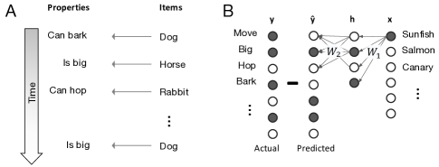
The network’s task is to predict an item’s properties ${\bf y}$ from its perceptual representation ${\bf x}$. These predictions are generated by propagating activity through a three layer linear neural network (Fig. 1B). The input activity pattern ${\bf x}$ in the first layer propagates through a synaptic weight matrix ${{\bf W}^{1}}$ of size $N_{2}\times N_{1}$, to create an activity pattern ${\bf h}={{\bf W}^{1}}{\bf x}$ in the second layer of $N_{2}$ neurons. We call this layer the “hidden” layer because it corresponds neither to input nor output. The hidden layer activity then propagates to the third layer through a second synaptic weight matrix ${{\bf W}^{2}}$ of size $N_{3}\times N_{2}$, producing an activity vector $\hat{\bf y}={{\bf W}^{2}}{\bf h}$ which constitutes the output prediction of the network. The composite function from input to output is thus simply $\hat{\bf y}={{\bf W}^{2}}{{\bf W}^{1}}{\bf x}$. For each input ${\bf x}$, the network compares its predicted output $\hat{\bf y}$ to the observed features ${\bf y}$ and it adjusts its weights so as to reduce the discrepancy between ${\bf y}$ and $\hat{\bf y}$.

To study the impact of depth, we will contrast the learning dynamics of this deep linear network to that of a shallow network that has just a single weight matrix, ${\bf W}^{s}$ of size $N_{3}\times N_{1}$ linking input activities directly to the network’s predictions $\hat{\bf y}={\bf W}^{s}{\bf x}$. At first inspection, it may seem that there is no utility whatsoever in considering deep linear networks, since the composition of linear functions remains linear. Indeed, the appeal of deep networks is thought to lie in the increasingly expressive functions they can represent by successively cascading many layers of nonlinear elements [38, 39]. In contrast, deep linear networks gain no expressive power from depth; a shallow network can compute any function that the deep network can, by simply taking ${\bf W}^{s}={{\bf W}^{2}}{{\bf W}^{1}}$. However, as we see below, the learning dynamics of the deep network is highly nonlinear, while the learning dynamics of the shallow network remains linear. Strikingly, many complex, nonlinear features of learning appear even in deep linear networks, and do not require neuronal nonlinearities.

As an illustration of the power of deep linear networks to capture learning dynamics even in nonlinear networks, we compare the two learning dynamics in Fig. 2. Fig. 2A shows a low dimensional visualization of the simulated learning dynamics of a multilayered nonlinear neural network trained to predict the properties of a set of items in a semantic domain of animals and plants (details of the neural architecture and training data can be found in [4]). The nonlinear network exhibits a striking, hierarchical progressive differentiation of structure in its internal hidden representations, in which animals versus plants are first distinguished, then birds versus fish, and trees versus flowers, and finally individual items. This remarkable phenomenon raises important questions about the theoretical principles governing the hierarchical differentiation of structure in neural networks. In particular, how and why do the network’s dynamics and the statistical structure of the input conspire to generate this phenomenon? In Fig. 2B we mathematically derive this phenomenon by finding analytic solutions to the nonlinear dynamics of learning in a deep linear network, when that network is exposed to a hierarchically structured semantic domain,

Figure 2: (A) A two dimensional multi-dimensional scaling (MDS) visualization of the temporal evolution of internal representations, across developmental time, of a deep nonlinear neural network studied in [4]. Reprinted from Figure 3.9, p. 113 of Ref [4]. Copyright © MIT Press, Permission Pending. (B) An MDS visualization of analytically derived learning trajectories of the internal representations of a deep linear network exposed to a hierarchically structured domain.

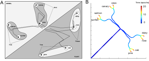
thereby shedding considerable theoretical insight onto the origins of hierarchical differentiation in a deep network. We present the derivation below, but for now, we note that the resemblance between Fig. 2A and Fig. 2B suggests that deep linear networks can form an excellent, analytically tractable model for shedding conceptual insight into the learning dynamics, if not the expressive power, of their nonlinear counterparts.

2 Acquiring Knowledge

We now begin an outline of the derivation that leads to Fig. 2B. The incremental error corrective process described above can be formalized as online stochastic gradient descent; each time an example $i$ is presented, the weights ${{\bf W}^{2}}$ and ${{\bf W}^{1}}$ are adjusted by a small amount in the direction that most rapidly decreases the squared error $\left\|{\bf y}^{i}-\hat{\bf y}^{i}\right\|^{2}$, yielding the standard back propagation learning rule

$$\Delta{{\bf W}^{1}}=\lambda{{\bf W}^{2}}^{T}\left({\bf y}^{i}-\hat{\bf y}^{i}\right){\bf x}^{iT},\,\,\Delta{{\bf W}^{2}}=\lambda\left({\bf y}^{i}-\hat{\bf y}^{i}\right){\bf h}^{iT},$$ (1)

where $\lambda$ is a small learning rate. This incremental update depends only on experience with a single item, leaving open the fundamental conceptual question of how and when the accumulation of such incremental updates can extract over developmental time, abstract structures, like hierarchical taxonomies, that are emergent properties of the entire domain of items and their features.

We show the extraction of such abstract domain structure is possible provided learning is gradual, with a small learning rate $\lambda$. In this regime, many examples are seen before the weights appreciably change, so learning is driven by the statistical structure of the domain. We imagine training is divided into a sequence of learning epochs. In each epoch the above rule is followed for all $P$ examples in random order. Then averaging (1) over all $P$ examples and taking a continuous time limit gives the mean change in weights per learning epoch,

$$\tau\frac{d}{dt}{{\bf W}^{1}} = {{\bf W}^{2}}^{T}\left({\bf\Sigma}^{yx}-{{\bf W}^{2}}{{\bf W}^{1}}{\bf\Sigma}^{x}\right),$$ (2)

$$\tau\frac{d}{dt}{{\bf W}^{2}} = \left({\bf\Sigma}^{yx}-{{\bf W}^{2}}{{\bf W}^{1}}{\bf\Sigma}^{x}\right){{\bf W}^{1}}^{T},$$ (3)

where ${\bf\Sigma}^{x}\equiv E[{\bf x}{\bf x}^{T}]$ is an $N_{1}\times N_{1}$ input correlation matrix, ${\bf\Sigma}^{yx}\equiv E[{\bf y}{\bf x}^{T}]$ is an $N_{3}\times N_{1}$ input-output correlation matrix, and $\tau\equiv\frac{1}{P\lambda}$ (see SI for detailed derivation). Here, $t$ measures time in units of learning epochs; as $t$ varies from 0 to 1, the network has seen $P$ examples corresponding to one learning epoch. These equations reveal that learning dynamics in even in our simple linear network can be highly complex: the second order statistics of inputs and outputs drives synaptic weight changes through coupled nonlinear differential equations with up to cubic interactions in the weights.

2.1 Explicit solutions from tabula rasa

These nonlinear dynamics are difficult to solve for arbitrary initial conditions on synaptic weights. However, we are interested in a particular limit: learning from a state of essentially no knowledge, which we model as small random synaptic weights. To further ease the analysis, we shall assume that the influence of perceptual correlations is minimal (${\bf\Sigma}^{x}\approx\bf I$). Our fundamental goal, then, is to understand the dynamics of learning in (2)-(3) as a function of the input-output correlation matrix ${\bf\Sigma}^{yx}$. The learning dynamics is closely related to terms in the singular value decomposition (SVD) of ${\bf\Sigma}^{yx}$ (Fig. 3A),

$${\bf\Sigma}^{yx}={\bf U}{\bf S}{\bf V}^{T}=\sum_{\alpha=1}^{N_{1}}s_{\alpha}{\bf u}^{\alpha}{\bf v}^{\alpha T},$$ (4)

which decomposes any matrix into the product of three matrices. Each of these matrices has a distinct semantic interpretation.

For example, the $\alpha$’th column ${\bf v}^{\alpha}$ of the $N_{1}\times N_{1}$ orthogonal matrix ${\bf V}$ can be thought of as an object analyzer vector; it determines the position of item $i$ along an important semantic dimension $\alpha$ in the training set through the component ${\bf v}^{\alpha}_{i}$. To illustrate this interpretation concretely, we consider a simple example dataset with four items (Canary, Salmon, Oak, and Rose) and five properties (Fig. 3). The two animals share the property can Move, while the two plants do not. Also each item has a unique property: can Fly, can Swim, has Bark, and has Petals. For this dataset, while the first row of ${\bf V}^{T}$ is a uniform mode, the second row, or the second object analyzer vector ${\bf v}^{2}$, determines where items sit on an animal-plant dimension, and hence has positive values for the Canary and Salmon and negative values for the plants. The other dimensions identified by the SVD are a bird-fish dimension, and a flower-tree dimension.

The corresponding $\alpha$’th column ${\bf u}^{\alpha}$ of the $N_{3}\times N_{3}$ orthogonal matrix ${\bf U}$ can be thought of as a feature synthesizer vector for semantic distinction $\alpha$. It’s components ${\bf u}^{\alpha}_{m}$ indicate the extent to which feature $m$ is present or absent in distinction $\alpha$. Hence the feature synthesizer ${\bf u}^{2}$ associated with the animal-plant semantic dimension has positive values for Move and negative values for Roots, as animals typically can move and do not have roots, while plants behave oppositely. Finally the $N_{3}\times N_{1}$ singular value matrix ${\bf S}$ has nonzero elements $s_{\alpha},\alpha=1,\ldots,N_{1}$ only on the diagonal, ordered so that $s_{1}\geq s_{2}\geq\cdots\geq s_{N_{1}}$. $s_{\alpha}$ captures the overall strength of the association between the $\alpha$’th input and output dimensions. The large singular value for the animal-plant dimension reflects the fact that this one dimension explains more of the training set than the finer-scale dimensions like bird-fish and flower-tree.

Figure 3: (A) Singular value decomposition (SVD) of input-output correlations. Associations between items and their properties are decomposed into modes. Each mode links a set of coherently covarying properties (a column of ${\bf U}$) with a set of coherently covarying items (a row of ${\bf V}^{T}$). The strength of the mode’s covariation is encoded by the singular value of the mode (diagonal element of ${\bf S}$). (B) Network input-output map, analyzed via the SVD. The effective singular values (diagonal elements of $A(t)$) evolve over time during learning. (C) Time-varying trajectories of the deep network’s effective singular values $a_{i}(t)$. Black dashed line marks the point in time depicted in panel B. (D) Time-varying trajectories of a shallow network’s effective singular values $b_{i}(t)$.

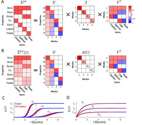
Given the SVD of the training set’s input-output correlation matrix in (4), we can now explicitly describe the network’s learning dynamics. The network’s overall input-output map at time $t$ is a time-dependent version of this SVD decomposition (Fig. 3B); it shares the object analyzer and feature synthesizer matrices of the SVD of ${\bf\Sigma}^{yx}$, but replaces the singular value matrix ${\bf S}$ with an effective singular value matrix $\and$,

$${{\bf W}^{2}}(t){{\bf W}^{1}}(t)={\bf U}\and{\bf V}^{T}=\sum_{\alpha=1}^{N_{2}}a_{\alpha}(t)\,{\bf u}^{\alpha}{\bf v}^{\alpha T},$$ (5)

where the trajectory of each effective singular value $a_{\alpha}(t)$ obeys

$$a_{\alpha}(t)=\frac{s_{\alpha}e^{2s_{\alpha}t/\tau}}{e^{2s_{\alpha}t/\tau}-1+s_{\alpha}/a_{\alpha}^{0}}.$$ (6)

Eqn. 6 describes a sigmoidal trajectory that begins at some initial value $a_{\alpha}^{0}$ at time $t=0$ and rises to $s_{\alpha}$ as $t\rightarrow\infty$, as plotted in Fig. 3C. This solution is applicable when the network begins as a tabula rasa, or an undifferentiated state with little initial knowledge, corresponding small random initial weights (see SI for derivation), and it provides an accurate description of the learning dynamics in this regime, as confirmed by simulation in Fig. 3C.

This solution also gives insight into how the internal representations in the hidden layer of the deep network evolve. An exact solution for ${{\bf W}^{2}}$ and ${{\bf W}^{1}}$ is given by

$${{\bf W}^{1}}(t)={\bf Q}\sqrt{\and}{\bf V}^{T},\qquad{{\bf W}^{2}}(t)={\bf U}\sqrt{\and}{\bf Q}^{-1},$$ (7)

where $\bf Q$ is an arbitrary $N_{2}\times N_{2}$ invertible matrix (SI Appendix). If initial weights are small, then the matrix $\bf Q$ will be close to orthogonal, i.e., ${\bf Q}\approx{\bf R}$ where ${\bf R}^{T}{\bf R}=\bf I$. Thus the internal representations are specified up to an arbitrary rotation ${\bf R}$. Factoring out the rotation, the hidden representation of item $i$ is

$$h^{\alpha}_{i}=\sqrt{a^{\alpha}(t)}{\bf v}_{i}^{\alpha}.$$ (8)

Thus internal representations develop over time by projecting inputs onto more and more input-output modes as they are learned.

The shallow network has a solution of analogous form, ${\bf W}^{s}(t)=\sum_{\alpha=1}^{\min(N_{1},N_{3})}b_{\alpha}(t)\,{\bf u}^{\alpha}{\bf v}^{\alpha T},$ but now each singular value evolves as

$$b_{\alpha}(t)=s_{\alpha}\left(1-e^{-t/\tau}\right)+b_{\alpha}^{0}e^{-t/\tau}.$$ (9)

In contrast to the deep network’s sigmoidal trajectory, Eqn. 9 describes a simple exponential approach from the initial value $b^{0}_{\alpha}$ to $s_{\alpha}$, as plotted in Fig. 3D. Hence depth fundamentally changes the dynamics of learning, yielding several important consequences below.

2.2 Rapid stage like transitions due to depth

We first compare the time-course of learning in deep versus shallow networks as revealed in Eqns. (6) and (9). For the deep network, beginning from a small initial condition $a_{\alpha}^{0}=\epsilon,$ each mode’s effective singular value $a_{\alpha}(t)$ rises to within $\epsilon$ of its final value $s_{\alpha}$ in time

$$t(s_{\alpha},\epsilon)=\frac{\tau}{s_{\alpha}}\ln\frac{s_{\alpha}}{\epsilon}$$ (10)

in the limit $\epsilon\rightarrow 0$ (SI Appendix). This is $O(1/s_{\alpha})$ up to a logarithmic factor. Hence modes with stronger explanatory power, as quantified by the singular value, are learned more quickly. Moreover, when starting from small initial weights, the sigmoidal transition from no knowledge of the mode to perfect knowledge can be arbitrarily sharp. Indeed the ratio of time spent in the sigmoidal transition regime to the ratio of time spent before making the transition can go to infinity as the initial weights go to zero (see SI Appendix). Thus rapid stage like transitions in learning can be prevalent even in deep linear networks.

By contrast, the timescale of learning for the shallow network is

$$t(s_{\alpha},\epsilon)=\tau\ln\frac{s_{\alpha}}{\epsilon},$$ (11)

which is $O(1)$ up to a logarithmic factor. Hence in a shallow network, the timescale of learning a mode depends only weakly on its associated singular value. Essentially all modes are learned at the same time, with an exponential rather than sigmoidal learning curve.

2.3 Progressive differentiation of hierarchical structure

We are now almost in a position to explain how we analytically derived the result in Fig. 2B. The only remaining ingredient is a mathematical description of the training data. Indeed the numerical results in Fig. 2A arose from a toy-training set, making it difficult to understand which aspects the data were essential for the hierarchical learning dynamics. Here, we introduce a probabilistic generative model for hierarchically structured data, in order to move beyond toy datasets to extract general principles of how statistical structure impacts learning.

We use a generative model (introduced in [40]) that mimics the process of evolution to create a dataset with explicit hierarchical structure (see SI Appendix). In the model, each feature diffuses down an evolutionary tree (Fig. 4A), with a small probability of mutating along each branch. The items lie at the leaves of the tree, and the generative process creates a hierarchical similarity matrix between items such that items with a more recent common ancestor on the tree are more similar to each other (Fig. 4B). We analytically computed the SVD of this hierarchical dataset and we found that the object analyzer vectors, which can be viewed as functions on the leaves of the tree in Fig. 4C respect the hierarchical branches of the tree, with the larger (smaller) singular values corresponding to broader (finer) distinctions. Moreover, in Fig. 4A we have artificially labelled the leaves and branches of the evolutionary tree with organisms and categories that might reflect a natural realization of this evolutionary process.

Figure 4: Hierarchy and the SVD. (A) A domain of eight items with an underlying hierarchical structure. (B) The correlation matrix of the features of the items. (C) Singular value decomposition of the correlations reveals semantic distinctions that mirror the hierarchical taxonomy. This is a general property of the SVD of hierarchical data. (D) The singular values of each semantic distinction reveal its strength in the dataset, and control when it is learned.

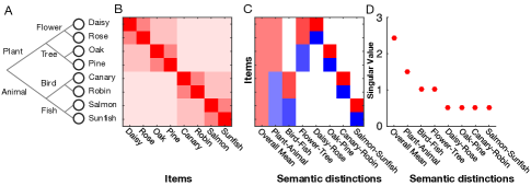
Now, inserting the singular values in Fig. 4D (and SI Appendix) into the deep learning dynamics in Eq. 6 to obtain the time-dependent singular values $a^{\alpha}(t)$, and then inserting these along with the object analyzers vectors ${\bf v}^{\alpha}$ in Fig. 4C into Eq. 8, we obtain a complete analytic derivation of the evolution of internal representations over developmental time in the deep network. An MDS visualization of these evolving hidden representation then yields Fig. 2B, which qualitatively recapitulates the much more complex network and dataset that led to Fig. 2A. In essence, this analysis completes a mathematical proof that the striking progressive differentiation of hierarchical observed in Fig. 2  is an inevitable consequence of deep learning dynamics, even in linear networks, when exposed to hierarchically structured data. The essential intuition is that dimensions of feature variation across items corresponding to broader (finer) hierarchical distinctions have stronger (weaker) statistical structure, as quantified by the singular values of the training data, and hence these dimensions are learned faster (slower), leading to waves of differentiation in a deep, but not a shallow network. Such a pattern of hierarchical differentiation has long been argued to apply to the conceptual development of infants and children [1, 5, 6, 7].

2.4 Illusory Correlations

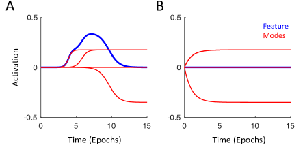
Another intriguing aspect of semantic development is that children sometimes attest to false beliefs (i.e. worms have bones [2]) that could not have been learned through direct experience. These errors challenge simple associationist accounts of semantic development that would predict a steady, monotonic accumulation of information about individual properties [16, 2, 41, 17]. Yet as shown in Fig. 5, the network’s knowledge of individual properties exhibits complex, non-monotonic trajectories over the course of learning. The overall prediction for a property is a sum of contributions from each mode, where the specific contribution of mode $\alpha$ to an individual feature $m$ for item $i$ is $a_{\alpha}(t){\bf u}^{\alpha}_{m}{\bf v}^{\alpha}_{i}$. In the example of Fig. 5A, the first two modes make a positive contribution while the third makes a negative one, yielding the inverted U-shaped trajectory.

Indeed, any property-item combination for which ${\bf u}^{\alpha}_{m}{\bf v}^{\alpha}_{i}$ takes different signs across different $\alpha$ will exhibit a non-monotonic learning curve, making such curves a frequent occurrence even in a fixed, unchanging environment. In a deep network, two modes with singular values that differ by $\Delta$ will have an interval in which the first is learned but the second is not. The length of this developmental interval is roughly $O(\Delta)$ (SI Appendix). Moreover, the rapidity of the deep network’s stage-like transitions further accentuates the non-monotonic learning of individual properties. This behavior, which may seem hard to reconcile with an incremental, error-corrective learning process, is a natural consequence of minimizing global rather than local prediction error: the fastest possible improvement in predicting all properties across all items sometimes results in a transient increase in the size of errors on specific items and properties. Every property in a shallow network, by contrast, monotonically approaches its correct value and therefore shallow networks provably never exhibit illusory correlations (SI Appendix).

Figure 5: Illusory correlations during learning. (A) Predicted value (blue) of feature “Can Fly” for item “Salmon” over the course of learning in a deep network (dataset as in Fig. 3). The contributions from each input-output mode are shown in red. (B) The predicted value and modes for the same feature in a shallow network.

3 Organizing and Encoding Knowledge

We now turn from the dynamics of learning to its final outcome. When exposed to a variety of items and features interlinked by an underlying hierarchy, for instance, what categories naturally emerge? Which items are particularly representative of a categorical distinction? And how is the structure of the domain internally represented?

3.1 Category membership, typicality, and prototypes

A long observed empirical finding is that category membership is not simply a logical, binary variable, but rather a graded quantity, with some objects being more or less typical members of a category (i.e. a sparrow is a more typical bird than a penguin). Indeed, such graded judgements of category membership are both highly reproducible across individuals [8, 9] and moreover correlate with performance on a range of tasks: subjects more quickly verify the category membership of more typical items [10, 11], more frequently recall typical examples of a category [12], and more readily extend new information about typical items to all members of a category [13, 14]. Our theoretical framework provides a natural mathematical definition of item typicality that both explains how it emerges from the statistical structure of the environment and improves task performance.

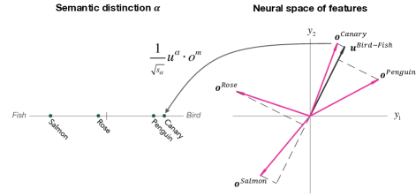
Indeed, a natural notion of the typicality of an item $i$ for a categorical distinction $\alpha$ is simply the quantity ${\bf v}^{\alpha}_{i}$ in the corresponding object analyzer vector. To see why this is natural, note that after learning, the neural network’s internal representation space has a semantic distinction axis $\alpha$, and each object $i$ is placed along this axis at a coordinate proportional to ${\bf v}^{\alpha}_{i}$, as seen in Eq. (8). Thus according to our definition, extremal points along this axis are the most typical members of a category. For example, if $\alpha$ corresponds to the bird-fish axis, objects $i$ with large positive ${\bf v}^{\alpha}_{i}$ are typical birds, while objects $i$ with large negative ${\bf v}^{\alpha}_{i}$ are typical fish. Also, the contribution of the network’s output to feature neuron $m$ in response to object $i$, from the hidden representation axis $\alpha$ alone is given by

$$\hat{\bf y}^{\alpha}_{m}\leftarrow{\bf u}^{\alpha}_{m}s_{\alpha}{\bf v}^{\alpha}_{i}.$$ (12)

Hence under our definition of typicality, an item $i$ that is more typical than another other item $j$ will have $|{\bf v}^{\alpha}_{i}|>|{\bf v}^{\alpha}_{j}|$, and thus will necessarily have a larger response magnitude under Eq. (12). Any performance measure which is monotonic in the response will therefore increase for more typical items under this definition. Thus our definition of item typicality is both a mathematically well defined function of the statistical structure of experience, through the SVD, and proveably correlates with task performance in our network.

Several previous attempts at defining the typicality of an item involve computing a weighted sum of category specific features present or absent in the item [42, 43, 8, 44, 15]. For instance, a sparrow is a more typical bird than a penguin because it shares more relevant features (can fly) with other birds. However, the specific choice of which features are relevant–the weights in the weighted sum of features–has often been heuristically chosen and relied on prior knowledge of which items belong to each category [8, 43]. Our definition of typicality can also be described in terms of a weighted sum of an object’s features, but the weightings are uniquely fixed by the statistics of the entire environment through the SVD (see SI Appendix):

$${\bf v}^{\alpha}_{i} = \frac{1}{Ps_{\alpha}}\sum_{m=1}^{N_{3}}{\bf u}^{\alpha}_{m}{\bf o}^{i}_{m},$$ (13)

which holds for all $i,m,$ and $\alpha$. Here, item $i$ is defined by its feature vector ${\bf o}^{i}\in R^{N_{3}}$, where component ${\bf o}^{i}_{m}$ encodes the value of its $m^{th}$ feature. Thus the typicality ${\bf v}^{\alpha}_{i}$ of item $i$ in distinction $\alpha$ can be computed by taking a weighted sum of the components of its feature vector ${\bf o}^{i}$, where the weightings are precisely the coefficients of the corresponding feature synthesizer vector ${\bf u}^{\alpha}$ (scaled by the reciprocal of the singular value). The neural geometry of Eq. 13 is illustrated in Fig. 6 when $\alpha$ corresponds to the bird-fish categorical distinction.

In many theories of typicality, the particular weighting of object features corresponds to a prototypical object [15, 3], or the best example of a particular category. Such object prototypes are often obtained by a weighted average over the feature vectors for the objects in a category (i.e. averaging together the features of all birds, for instance, will give a set of features they share). However, such an average relies on prior knowledge of the extent to which an object belongs to a category. Our theoretical framework also yields a natural notion of object prototypes as a weighted average of object feature vectors, but unlike many other frameworks, it yields a unique prescription for the object weightings in terms of the statistical structure of the environment through the SVD (SI Appendix):

$${\bf u}^{\alpha}_{m} = \frac{1}{Ps_{\alpha}}\sum_{i=1}^{N_{1}}{\bf v}^{\alpha}_{i}{\bf o}^{i}_{m}.$$ (14)

Thus the feature synthesizer ${\bf u}^{\alpha}$, can itself be thought of as a category prototype for distinction $\alpha$, as it can be obtained through a weighted average of all the object feature vectors ${\bf o}^{i}$, where the weighting of object $i$ is none other than the typicality ${\bf v}^{\alpha}_{i}$ of object $i$ in distinction $\alpha$. In essence, each element ${\bf u}^{\alpha}_{m}$ of the prototype vector signifies how important feature $m$ is for distinction $\alpha$ (Fig. 6).

In summary, a beautiful and simple duality between item typicality and category prototypes arises as an emergent property of the learned internal representations of the neural network. The typicality of an item is determined by the projection of that item’s feature vector onto the category prototype in (13). And the category prototype is an average over all object feature vectors, weighted by their typicality in (14). Moreover, in any categorical distinction $\alpha$, the most typical items $i$ and the most important features $m$ are determined by the extremal values of ${\bf v}^{\alpha}_{i}$ and ${\bf u}^{\alpha}_{m}$.

Figure 6: The geometry of item typicality. For a semantic distinction $\alpha$ (in this case $\alpha$ is the bird-fish distinction) the object analyzer vector ${\bf v}^{\alpha}_{i}$ arranges objects $i$ along an internal neural representation space where the most typical birds take the extremal positive coordinates, and the most typical fish take the extremal negative coordinates. Objects like a rose, that is neither a bird nor a fish, are located near the origin on this axis. Positions along the neural semantic axis can also be obtained by computing the inner product between the feature vector ${\bf o}^{i}$ for object $i$ and the feature synthesizer ${\bf u}^{\alpha}$ as in (13). Moreover ${\bf u}^{\alpha}$ can be thought of as a category prototype for semantic distinction $\alpha$ through (14).

3.2 Category coherence

The categories we naturally learn are not arbitrary, but instead are in some sense coherent, and efficiently represent the structure of the world [8, 15, 16]. For example, the set of things that are are Red and cannot Swim, is a well defined category, but intuitively is not as coherent as the category of Dogs; we naturally learn, and even name, the latter category, but not the former. When is a category learned at all, and what determines its coherence? An influential proposal [8, 15] suggested that coherent categories consist of tight clusters of items that share many features, and moreover are highly distinct from other categories with different sets of shared features. Such a definition, as noted in [3, 16, 17] can be circular: to know which items are category members, one must know which features are important for that category, and conversely, to know which features are important, one must know which items are members. Thus a mathematical definition of category coherence, as a function of the statistical structure of the environment, that is proveably related to the learnability of categories by neural networks, has remained elusive.

Here we provide such a definition for a simple model of disjoint categories, and demonstrate how neural networks can cut through the Gordian knot of circularity. Our definition and theory is motivated by, and consistent with, prior network simulations exploring notions of category coherence through the coherent covariation of features [4].

Figure 7: The discovery of disjoint categories buried in noise. (A) A data set of $N_{0}=1000$ items and $N_{f}=1600$ features, with no discernible visible structure. (B) Yet when a deep linear network learns to predict the features of items, an MDS visualization of the evolution of its internal representations reveals $3$ clusters. (C) By computing the SVD of the product of synaptic weights ${{\bf W}^{2}}{{\bf W}^{1}}$, we can extract the network’s object analyzers ${\bf v}^{\alpha}$ and feature synthesizers ${\bf u}^{\alpha}$, finding $3$ with large singular values $s_{\alpha}$, for $\alpha=1,\dots,3$. Each of these $3$ object analyzers ${\bf v}^{\alpha}$ and feature synthesizers ${\bf u}^{\alpha}$ takes large values on a subset of items and features respectively, and we can use them to reorder the rows and columns of (A) to obtain (C). This re-ordering reveals underlying structure in the data corresponding to $3$ disjoint categories, such that if a feature and item belong to a category, the feature is present with a high probability $p$, whereas if it does not, it appears with a low probability $q$. (D) Thus intuitively, the dataset corresponds to $3$ clusters buried in a noise of irrelevant objects and features. (E) Performance in recovering one such category can be measured by computing the correlation coefficients between the object analyzer and feature synthesizer returned by the network to the ideal object analyzer ${\bf v}^{\text{Ideal}}$ and ideal feature synthesizer ${\bf u}^{\text{Ideal}}$ that take nonzero values on the items and features, respectively, that are part of the category, and are zero on the rest of the items and features. This learning performance, for the object analyzer, is shown for various parameter values. Solid curves are analytical theory derived from a random matrix analysis (SI Appendix) and data points are obtained from simulations. (F) All performance curves in (E) collapse onto a single theoretically predicted, universal learning curve, when measured in terms of the category coherence defined in Eq. 15.

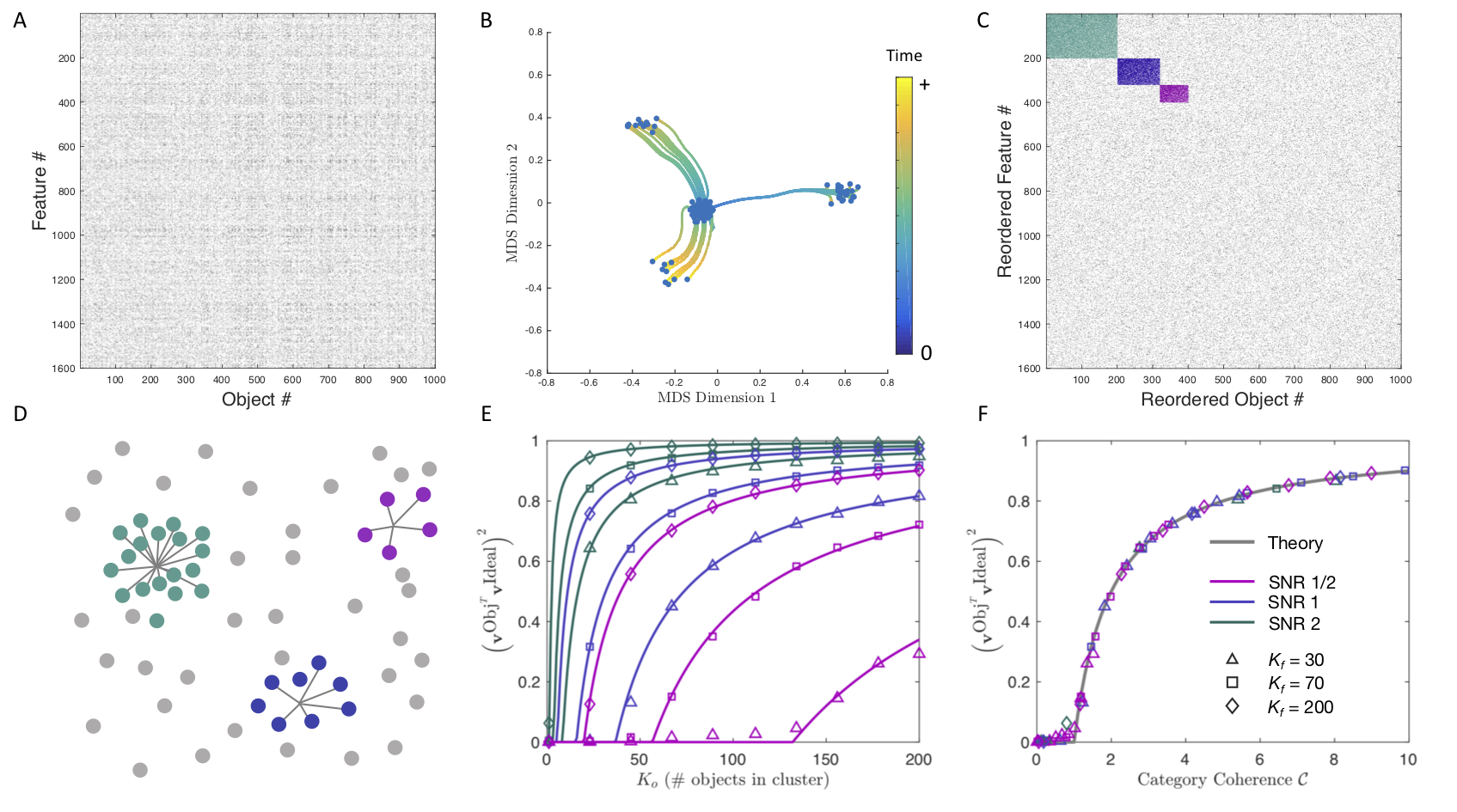
Consider for example, a dataset consisting of $N_{o}$ objects and $N_{f}$ features. Now consider a category consisting of a subset of $K_{f}$ features that tend to occur with high probability $p$ in a subset of $K_{o}$ items, whereas a background feature occurs with a lower probability $q$ in a background item $p$ when either are not part of the category. For what values of $K_{f}$, $K_{0}$, $p$, $q$, $N_{f}$ and $N_{0}$ can such a category be learned, and if so, how accurately? Fig. 7A-D illustrates, for example, how a neural network can extract $3$ such categories buried in the background noise. We see in Fig. 7E that the performance of category extraction increases as the number of items $K_{0}$ and features $K_{f}$ in the category increases, and also as the signal-to-noise ratio, or $\text{SNR}\equiv\frac{(p-q)^{2}}{q(1-q)}$ increases. Through random matrix theory (SI Appendix), we show that performance depends on the various parameters $\it{only}$ through a category coherence variable

$$\mathcal{C}=\text{SNR}\frac{K_{o}K_{f}}{\sqrt{N_{o}N_{f}}}.$$ (15)

When the performance curves in Fig. 7E are re-plotted with category coherence $\mathcal{C}$ on the horizontal axis, all the curves collapse onto a single universal performance curve shown in Fig. 7F. We derive a mathematical expression for this curve in SI Appendix. It displays an interesting threshold behavior: if the coherence $\mathcal{C}\leq 1$, the category is not learned at all, and the higher the coherence above this threshold, the better the category is learned.

This threshold is strikingly permissive. For example, at $\text{SNR}=1$, it occurs at $K_{0}K_{f}=\sqrt{N_{0}N_{f}}$. Thus in a large environment of $N_{o}=1000$ objects and $N_{f}=1600$ features, as in Fig. 7A, a small category of $40$ objects and $40$ features can be easily learned, even by a simple deep linear network. Moreover, this analysis demonstrates how the deep network solves the problem of circularity described above by simultaneously bootstrapping the learning of object analyzers and feature synthesizers in its synaptic weights. Finally, we note that the definition of category coherence in Eq. (15) is qualitatively consistent with previous notions; coherent categories consist of large subsets of items possessing, with high probability, large subsets of features that tend not to co-occur in other categories. However, our quantitative definition has the advantage that it proveably governs category learning performance in a neural network.

3.3 Basic categories

Closely related to category coherence, a variety of studies of naming have revealed a privileged role for basic categories at an intermediate level of specificity (i.e. Bird), compared to superordinate (i.e. Animal) or subordinate (i.e. Robin) levels. At this basic level, people are quicker at learning names [45, 46], prefer to generate names [46], and are quicker to verify the presence of named items in images [46, 11]. We note that basic level advantages typically involve naming tasks done at an older age, and so need not be inconsistent with progressive differentiation of categorical structure from superordinate to subordinate levels as revealed in preverbal cognition [1, 47, 5, 6, 7, 4]. Moreover, some items are named more frequently than others, and these frequency effects could contribute to a basic level advantage [4]. However in artificial category learning experiments where frequencies are tightly controlled, basic level categories are still often learned first [48]. What statistical properties of the environment could lead to this basic level effect? While several properties have been put forth in the literature [44, 48, 11, 42], a mathematical function of environmental structure that proveably confers a basic level advantage to neural networks has remained elusive.

Here we provide such a function by generalizing the notion of category coherence $\mathcal{C}$ in the previous section to hierarchically structured categories. Indeed, in any dataset containing strong categorical structure, so that its singular vectors are in one to one correspondence with categorical distinctions, we simply propose to define the coherence of a category by the associated singular value. This definition has the advantage of obeying the theorem that more coherent categories are learned faster, through Eq. (6). Moreover, we show in SI Appendix that this definition is consistent with that of category coherence $\mathcal{C}$ defined in Eq. (15) for the special case of disjoint categories. However, for hierarchically structured categories as in Fig. 4, this singular value definition always predicts an advantage for superordinate categories, relative to basic or subordinate.

Is there an alternate statistical structure for hierarchical categories that confers high category coherence at lower levels in the hierarchy? We exhibit two such structures in Fig. 8. More generally, in the SI Appendix, we analytically compute the singular values at each level of the hierarchy in terms of the similarity structure of items. We find these singular values are a weighted sum of within cluster similarity minus between cluster similarity for all levels below, weighted by the fraction of items that are descendants of that level. If at any level, between cluster similarity is negative, that detracts from the coherence of superordinate categories, contributes strongly to the coherence of categories at that level, and does not contribute to subordinate categories.

Figure 8: From hierarchical similarity structure to category coherence. (A) A hierarchical similarity structure over objects in which categories at the basic level are very different from each other due to a negative similarity. (B) For such similarity structure, basic level categorical distinctions acquire larger singular values, or category coherence, and therefore gain an advantage in both learning and in task performance. (C) Now subordinate categories are very different from each other through negative similarity. (D) Consequently, subordinate categories gain a coherence advantage. See SI Appendix for analytic formulas relating similarity structure to category coherence.

Thus the singular value based definition of category coherence is qualitatively consistent with prior intuitive notions. For instance, paraphrasing Keil (1991), coherent categories are clusters of tight bundles of features separated by relatively empty spaces [17]. Also, consistent with [16, 17, 3], we note that we cannot judge the coherence of a category without knowing about its relations to all other categories, as singular values are a complex emergent property of the entire environment. But going beyond past intuitive notions, our quantitative definition of category coherence based on singular values enables us to prove that coherent categories are most easily and quickly learned, and also proveably provide the most accurate and efficient linear representation of the environment, due to the global optimality properties of the SVD (see SI Appendix for details).

3.4 Discovering and representing explicit structures

While we have focused on hierarchical structure, the world may contain many different types of abstract structures. How are these different structures learned and encoded by neural networks? A convenient formalization of environmental structure can be specified in terms of a probabilistic graphical model (PGM), defined by a graph over items (Fig. 9  top) that can express a variety of structural forms underlying a domain, including clusters, trees, rings, grids, orderings, and hierarchies. Features are assigned to items by independently sampling from the PGM (see [29] and SI Appendix), such that nearby items in the graph are more likely to share features. For each of

Figure 9: Representation of explicit structural forms in a neural network. Each column shows a different structure. The first four columns correspond to pure structural forms, while the final column has cross-cutting structure. First row: The structure of the data generating probabilistic graphical model (PGM). Second row: The resulting item covariance matrix arising from either data drawn from the PGM (first four columns) or designed by hand (final column). Third row: The input-analyzing singular vectors that will be learned by the linear neural network. Each vector is scaled by its singular value, showing its importance to representing the covariance matrix. Fourth row: MDS view of the development of internal representations.

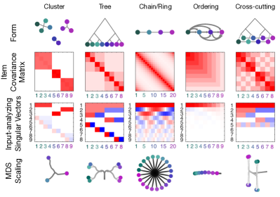
these structural forms, in the limit of a large number of features, we computed the item-item covariance matrices (Fig. 9  second row), object analyzer vectors (Fig. 9  third row) and singular values of the resultant input-output correlation matrix, and we employed them in our learning dynamics in Eq. 6 to compute the development of the network’s internal representations through Eq. 8. These evolving hidden representations are shown in (Fig. 9  bottom). Overall, this approach yields several insights into how distinct structural forms, through their different statistics, drive learning in a deep network, as summarized below:

Clusters.

Graphs that break items into distinct clusters give rise to block-diagonal constant matrices, yielding object-analyzer vectors that pick out cluster membership.

Trees.

Tree graphs give rise to ultrametric covariance matrices, yielding object-analyzer vectors that are tree-structured wavelets that mirror the underlying hierarchy [49, 50].

Rings and Grids.

Ring-structured graphs give rise to circulant covariance matrices, yielding object-analyzer vectors that are Fourier modes ordered from lowest to highest frequency [51].

Orderings.

Graphs that transitively order items yield highly structured, but non-standard, covariance matrices whose object analyzers encode the ordering.

Cross-cutting Structure.

Real-world domains need not have a single underlying structural form. For instance, while some features of animals and plants generally follow a hierarchical structure, other features like male and female can link together hierarchically disparate items. Such cross-cutting structure can be orthogonal to the hierarchical structure, yielding object-analyzer vectors that span hierarchical distinctions.

In essence, these results reflect an analytic link between two very popular, but different, methods of capturing structure: PGM’s and deep networks. This general analysis transcends the particulars of any one dataset, and shows how different abstract structures become embedded in the internal representations of a deep neural network.

4 Deploying Knowledge: Inductive Projection

Over the course of development, the knowledge acquired by children powerfully reshapes their inductions upon encountering novel items and properties [2, 3]. For instance, upon learning a novel fact (e.g., “a canary is warm-blooded”) children extend this new knowledge to related items, as revealed by their answers to questions like ”is a robin warm-blooded?” Studies of inductive projection have shown that children’s answers to such questions change over the course of development [2, 18, 17, 3, 19], generally becoming more specific with age. For example, young children may readily project the novel property of warm-blooded to distantly related items, while older children will only project it to more closely related items. How could such changing patterns of inductive generalization arise in a neural network? Here, building upon previous network simulations of inductive projection [31, 4], we show analytically that deep networks exposed to hierarchically structured data, naturally yield progressively narrowing patterns of inductive projection across development.

Figure 10: The neural geometry of inductive generalization. (A) A novel feature (property x) is observed for a familiar item (i.e. ”a pine has property x”). (B) Learning assigns the novel feature a neural representation in the hidden layer of the network that places it in semantic similarity space near the object which possesses the novel feature. The network then inductively projects that novel feature to other familiar items (e.g. ”Does a rose have property x?”) only if their hidden representation is close in neural space. (C) A novel item (a blick) possesses a familiar feature (i.e. ”a blick can move”). (D) Learning assigns the novel item a neural representation in the hidden layer that places it in semantic similarity space near the feature possessed by the novel item. Other features are inductively projected to that item (e.g., ”Does a blick have wings?”) only if their hidden representation is close in neural space. (E) Inductive projection of a novel property (”a pine has property x”) over learning. As learning progresses, the neural representations of items become progressively differentiated, yielding progressively restricted projection of the novel feature to other items. Here the pine can be thought of as the left-most item node in the tree.

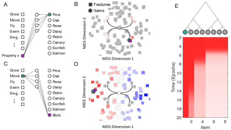
Consider the act of learning that a familiar item has a novel feature (e.g. “a pine has property x”). To accommodate this knowledge, new synaptic weights must be chosen between the familiar item pine and the novel property x (Fig. 10A), without disrupting prior knowledge of items and their properties already stored in the network. This may be accomplished by adjusting only the weights from the hidden layer to the novel feature so as to activate it appropriately. With these new weights established, inductive projections of the novel feature to other familiar items (e.g. “does a rose have property x?”) naturally arise by querying the network with other inputs. If a novel property $m$ is ascribed to a familiar item $i$, the inductive projection of this property to any other item $j$ is given by (see SI Appendix),

$$\hat{\bf y}_{m}={\bf h}_{j}^{T}{\bf h}_{i}/\left\|{\bf h}_{i}\right\|^{2}.$$ (16)

This equation implements a similarity-based inductive projection of the novel property to other items, where the similarity metric is precisely the Euclidean similarity of hidden representations of pairs of items (Fig. 10B). In essence, being told “a pine has property x,” the network will more readily project the novel property x to those familiar items whose hidden representations are close to that of the pine.

A parallel situation arises upon learning that a novel item possesses a familiar feature (e.g., “a blick can move,” Fig. 10C). Encoding this knowledge requires new synaptic weights between the item and the hidden layer. Appropriate weights may be found through standard gradient descent learning of the item-to-hidden weights for this novel item, while holding the hidden-to-output weights fixed to preserve prior knowledge about features. The network can then inductively project other familiar properties to the novel item (e.g., ”Does a blick have legs?”) by simply generating a feature output vector in response to the novel item as input. Under this scheme, a novel item $i$ with a familiar feature $m$ will be assigned another familiar feature $n$ through the equation (SI Appendix),

$$\hat{\bf y}_{n}={\bf h}_{n}^{T}{\bf h}_{m}/\left\|{\bf h}_{m}\right\|^{2},$$ (17)

where the $\alpha^{th}$ component of ${\bf h}_{n}$ is ${\bf h}_{n}^{\alpha}={\bf u}^{\alpha}_{n}\sqrt{a_{\alpha}(t)}$. ${\bf h}_{n}\in{\bf R}^{N_{2}}$ can be thought of as the hidden representation of feature $n$ at developmental time $t$. In parallel to (16), this equation now implements similarity based inductive projection of familiar features to a novel item. In essence, being told “a blick can move,” the network will more readily project other familiar features to a blick, if those features have a similar internal representation as that of the feature move.

Thus the hidden layer of the deep network furnishes a common, semantic representational space into which both features and items can be placed. When a novel feature $m$ is assigned to a familiar item $i$, that novel feature is placed close to the familiar item in the hidden layer, and so the network will inductively project this novel feature to other items close to $i$ in neural space. In parallel, when a novel item $i$ is assigned a familiar feature $m$, that novel item is placed close to the familiar feature, and so the network will inductively project other features close to $m$ in neural space, onto the novel item.

This principle of similarity based generalization encapsulated in Eqns. 16 and 17, when combined with the progressive differentiation of internal representations over developmental time as the network is exposed to hierarchically structured data, as illustrated in Fig. 2B, then naturally explains the shift in patterns of inductive projection from broad to specific across development, as shown in Fig. 10E. For example, consider specifically the inductive projection of a novel feature to familiar items (Fig. 10AB). Earlier (later) in developmental time, neural representations of all items are more similar to (different from) each other, and so the network similarity based inductive projection will extend the novel feature to many (fewer) items, thereby exhibiting progressively narrower patterns of inductive projection that respect the hierarchical similarity structure of the environment (Fig. 10E). Thus remarkably, even a deep linear network can provably exhibit the same broad to specific changes in patterns of inductive projection that are empirically observed in many works [2, 18, 17, 3].

5 Linking Behavior and Neural Representations

Compared to previous models which have primarily made behavioral predictions, our theory has a clear neural interpretation. Here we discuss implications for the neural basis of semantic cognition.

5.1 Similarity structure is an invariant of optimal learning

An influential method for probing neural codes for semantic knowledge in empirical measurements of neural activity is the representational similarity approach (RSA) [20, 52, 28, 21], which examines the similarity structure of neural population vectors in response to different stimuli. This technique has identified rich structure in high level visual cortices, where, for instance, inanimate objects are differentiated from animate objects [22, 23, 24, 25, 26]. Strikingly, studies have found remarkable constancy between neural similarity structures across human subjects, and even between humans and monkeys [27, 28]. This highly conserved similarity structure emerges despite considerable variability in neural activity patterns across subjects [53, 54]. Indeed, exploiting similarity structure enables more effective across-subject decoding of fMRI data relative to transferring a decoder based on careful anatomical alignment [55]. Why is representational similarity conserved, both across individuals and species, despite highly variable tuning of individual neurons and anatomical differences?

Remarkably, we show that two networks trained in the same environment must have identical representational similarity matrices despite having detailed differences in neural tuning patterns, provided that the learning process is optimal, in the sense that it yields the smallest norm weights that solve the task (see SI Appendix for a derivation). One way to get close to the optimal manifold of synaptic weights of smallest norm after learning, is to start learning from small random initial weights. We show in Fig. 11AB that two networks, each starting from different sets of small

Figure 11: Neural representations and invariants of learning. Columns A-B depict two networks trained from small norm random weights. Columns C-D depict two networks trained from large norm random weights. Top row: Neural tuning curves $h_{i}$ at the end of learning. Neurons show mixed selectivity tuning, and individual tuning curves are different for different trained networks. Middle row: Representational similarity matrix ${\bf\Sigma}^{h}$. Bottom row: Behavioral similarity matrix ${\bf\Sigma}^{\hat{y}}$. For small-norm, but not large-norm weight initializations, representational similarity is conserved and behavioral similarity mirrors neural similarity.

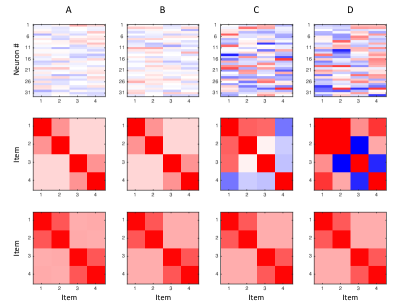
random initial weights, will after training learn very different internal representations (Fig. 11AB top row) but will have nearly identical representational similarity matrices (Fig. 11AB middle row). Such a result is however, not obligatory. Two networks starting from large random initial weights not only learn different internal representations, but also learn different representational similarity matrices (Fig. 11CD top and middle rows). This pair of networks both learn the same composite input output map, but with suboptimal large-norm weights. Hence our theory, combined with the empirical finding that similarity structure is preserved across humans and species, may speculatively suggest that all these disparate neural circuits may be implementing an approximately optimal learning process in a common environment.

5.2 When the brain mirrors behavior

In addition to matching neural similarity patterns across subjects, experiments using fMRI and single unit responses have also documented a correspondence between neural similarity patterns and behavioral similarity patterns [21]. When does neural similarity mirror behavioral similarity? We show this correspondence again emerges only in optimal networks.

In particular, denote by $\hat{\bf y}_{i}$ the behavioral output of the network in response to item $i$. These output patterns yield the behavioral similarity matrix ${\bf\Sigma}^{\hat{y}}_{ij}=\hat{\bf y}_{i}^{T}\hat{\bf y}_{j}$. In contrast, the neural similarity matrix is ${\bf\Sigma}^{h}_{ij}={\bf h}_{i}^{T}{\bf h}_{j}$ where ${\bf h}_{i}$ is the hidden representation of stimulus $i$. We show in the SI Appendix that if the network learns optimal smallest norm weights, then these two similarity matrices obey the relation

$${\bf\Sigma}^{\hat{y}}=\left({\bf\Sigma}^{h}\right)^{2}.$$ (18)

Moreover, we show the two matrices share the same singular vectors. Hence behavioral similarity patterns share the same structure as neural similarity patterns, but with each semantic distinction expressed more strongly (according to the square of its singular value) in behavior relative to the neural representation. While this precise mathematical relation is yet to be tested in detail, some evidence points to this greater category separation in behavior [27].

Given that optimal learning is a prerequisite for neural similarity mirroring behavioral similarity, as in the previous section, there is a match between the two for pairs of networks trained from small random initial weights (Fig. 11AB middle and bottom rows), but not for pairs of networks trained from large random initial weights (Fig. 11CD middle and bottom rows). Thus again, speculatively, our theory suggests that the experimental observation of a link between behavioral and neural similarity may in fact indicate that learning in the brain is finding optimal network solutions that efficiently implement the requisite transformations with minimal synaptic strengths.

6 Discussion

In summary, the main contribution of our work is the analysis of a simple model, namely a deep linear neural network, that can, surprisingly, qualitatively capture a diverse array of phenomena in semantic development and cognition. Our exact analytical solutions of nonlinear learning phenomena in this model yield conceptual insights into why such phenomena also occur in more complex nonlinear networks [4, 31, 32, 33, 34, 35, 36, 37] trained to solve semantic tasks. In particular, we find that the hierarchical differentiation of internal representations in a deep, but not a shallow, network (Fig. 2) is an inevitable consequence of the fact that singular values of the input-output correlation matrix drive the timing of rapid developmental transitions (Fig. 3 and Eqns. (6) and (10)), and hierarchically structured data contains a hierarchy of singular values (Fig. 4). In turn, semantic illusions can be highly prevalent between these rapid transitions simply because global optimality in predicting all features of all items necessitates sacrificing correctness in predicting some features of some items (Fig. 5). And finally, this hierarchical differentiation of concepts is intimately tied to the progressive sharpening of inductive generalizations made by the network (Fig. 10).

The encoding of knowledge in the neural network after learning also reveals precise mathematical definitions of several aspects of semantic cognition. Basically, the synaptic weights of the neural network extract from the statistical structure of the environment a set of paired object analyzers and feature synthesizers associated with every categorical distinction. The bootstrapped, simultaneous learning of each pair solves the apparent Gordian knot of knowing both which items belong to a category, and which features are important for that category: the object analyzers determine category membership, while the feature synthesizers determine feature importance, and the set of extracted categories are uniquely determined by the statistics of the environment. Moreover, by defining the typicality of an item for a category as the strength of that item in the category’s object analyzer, we can prove that typical items must enjoy enhanced performance in semantic tasks relative to atypical items (Eq. (12)). Also, by defining the category prototype to be the associated feature synthesizer, we can prove that the most typical items for a category are those that have the most extremal projections onto the category prototype (Fig. 6 and Eq. 13 ). Finally, by defining the coherence of a category to be the associated singular value, we can prove that more coherent categories can be learned more easily and rapidly (Fig. 7) and explain how changes in the statistical structure of the environment determine what level of a category hierarchy is the most basic or important (Fig. 8). All our definitions of typicality, prototypes and category coherence are broadly consistent with intuitions articulated in a wealth of psychology literature, but our definitions imbue these intuitions with enough mathematical precision to prove theorems connecting them to aspects of category learnability, learning speed and semantic task performance in a neural network model.

More generally, beyond categorical structure, our analysis provides a principled framework for explaining how the statistical structure of diverse structural forms associated with different probabilistic graphical models gradually become encoded in the weights of a neural network (Fig. 9). Also, with regards to neural representation, our theory reveals that across different networks trained to solve a task, while there may be no correspondence at the level of single neurons, the similarity structure of internal representations of any two networks will both be identical to each other, and closely related to the similarity structure of behavior, provided both networks solve the task optimally, with the smallest possible synaptic weights. Neither correspondence is obligatory, in that both need not hold for suboptimal networks (Fig. 11). This result suggests, but by no means proves, that the neural and behavioral alignment of similarity structure in human and monkey IT may be a consequence of each circuit finding optimal solutions to similar tasks.

While our simple neural network surprisingly captures this diversity of semantic phenomena in a mathematically tractable manner, because of its linearity, the phenomena it can capture still barely scratch the surface of semantic cognition. Some fundamental semantic phenomena that require complex nonlinear processing and memory include context dependent computations, dementia in damaged networks, theory of mind, the deduction of causal structure, and the binding of items to roles in events and situations. While it is inevitably the case that biological neural circuits exhibit all of these phenomena, it is not clear how our current generation of artificial nonlinear neural networks can recapitulate all of them. However, we hope that a deeper mathematical understanding of even the simple network presented here can serve as a springboard for the theoretical analysis of more complex neural circuits, which in turn may eventually shed much needed light on how the higher level computations of the mind can emerge from the biological wetware of the brain.