Charging the Johannsen-Psaltis spacetime

Abstract

In this paper we develop the charged version of the spacetime proposed by Johannsen and Psaltis. Rotation is introduced in the deformed Reissner-Nordström spacetime by complex coordinate transformation. The event horizon and Killing horizon are studied. Killing horizons are represented graphically also. The analysis of the determinant of the metric shows that the spacetime does not have Lorentz violating regions. Similarly, from the study of the closed time-like curves, we see that no such curves exist outside the central body. Expressions for the energy and angular momentum for a particle on the equatorial plane are determined. Location of the circular photon orbits and innermost stable circular orbits is also computed.

1 Introduction

It is a difficult task to find rotating solutions in the general theory of relativity which was given by Einstein in 1915. The van Stockum rotating solution vs was developed two decades later and it took more than forty years to discover the rotating solution of Kerr. According to the no-hair theorem 2a , solutions to the Einstein-Maxwell theory are uniquely described by the three parameters namely mass, charge and rotation. In the static and spherically symmetric setting the Schwarzschild and Reissner-Nordström are solutions to the Einstein field equations. The Kerr metric is the rotating generalization of the Schwarzschild solution and Kerr-Newman spacetime is the rotating generalization of the Reissner-Nordström solution as well as charged generalization of the Kerr metric. The Newman-Janis algorithm nj was used to develop exterior rotating solutions but later was applied for developing rotating interior metrics which were matched to the exterior Kerr intro1 . This algorithm is based on complex coordinate transformation. It introduces rotation into the static spacetimes. Kerr and Kerr-Newman spacetimes have been derived via Newman-Janis algorithm by using the Schwarzschild and Reissner-Nordström spacetimes as seed metrics respectively nj ; nj1 .

The general theory of relativity has been put to test extensively in numerous ways. One such test is to see that the black holes are described by the Kerr solution. This can be done in many ways 2b . Tests in the weak gravitational field regime can depend on the parameterized post-Newtonian approach 3 . On the contrary, one must model the black hole metric in terms of parametric deviations from the Kerr spacetime in order to take the test in strong gravitational regime. A number of such spacetimes have been developed 4b ; jp ; chern .

A particularly interesting modified Kerr spacetime has been proposed by Johannsen and Psaltis jp by applying the Newman-Janis algorithm to a deformed Schwarzschild metric. It is a stationary, axisymmetric, asymptotically flat vacuum solution of some unknown field equations differing from the Einstein field equations due to the presence of function $h(r,\theta)$. In addition to the spin and mass parameters, this metric contains at least one parameter which measures the potential deviations from the Kerr spacetime. Setting such deviation parameters to zero, one recovers the Kerr metric. It could be the ad-hoc starting point for the investigation of deviations from general relativity han . In case of modified theories of gravity, Newman-Janis formulation usually does not relate static solutions with corresponding stationary solutions but can be applied to modified forms of the Schwarzschild spacetime yunes .

Most known astrophysical compact objects are either electrically neutral or slightly charged. The Kerr-Newman black hole is an exact electro vacuum solution of the Einstein-Maxwell system of equations. It is an ideal model for the interaction between the electromagnetic field and the gravitoelectric and gravitomagnetic components of gravity. Therefore, it is significant both conceptually and theoretically. Keeping in view the Kerr-Newman metric of general relativity, we look for a rotating charged spacetime in the alternate theories of gravity. In the case of vector-tensor theories of alternate gravity, an exact rotating solution has been developed recently ft . The charged rotating solutions in the limit of small Weyl corrections was developed in Ref. weyl .

The main motivation for this work comes from the Johannsen-Psaltis spacetime. In this paper we take the deformed Reissner-Nordström spacetime as the seed metric and construct the charged generalization of the Johannsen-Psaltis spacetime.

This paper is organized as follows. In Section 2 the charged metric is developed. In Section 3 the event horizon and Killing horizon have been discussed. Section 4 analyzes our metric for the existence of Lorentz violation regions and closed time-like curves. The innermost stable circular orbits (ISCO) and circular photon orbits are computed in Section 5. The work is concluded in the last section.

2 The construction

The Reissner-Nordström metric is given by

$$ds^{2}=-\left(1-\frac{2M}{r}+\frac{q^{2}}{r^{2}}\right)dt^{2}+\left(1-\frac{2M}{r}+\frac{q^{2}}{r^{2}}\right)^{-1}dr^{2}+r^{2}d\theta^{2}+r^{2}\sin^{2}\theta d\phi^{2},$$ (1)

where $M$ is the mass of the central object having charge $q$. The 4-potential for the above metric is

$$A_{\mu}=\left(-\frac{q}{r},0,0,0\right).$$ (2)

The $(t-r)$ sector is modified by multiplying the corresponding component by the expression of the form $1+h(r)$ where $h(r)$ is given by jp

$$h(r)=\sum_{k=0}^{\infty}\epsilon_{k}\left(\frac{M}{r}\right)^{k}.$$ (3)

The deformed Reissner-Nordström spacetime thus takes the form

$$ds^{2} =-\left(1-\frac{2M}{r}+\frac{q^{2}}{r^{2}}\right)\Big{(}1+h(r)\Big{)}dt^{2}+\left(1-\frac{2M}{r}+\frac{q^{2}}{r^{2}}\right)^{-1}\Big{(}1+h(r)\Big{)}dr^{2}+r^{2}d\theta^{2}$$

$$+r^{2}\sin^{2}\theta d\phi^{2}.$$ (4)

Setting $\epsilon_{k}=0$ gives the Reissner-Nordström spacetime. First, let us denote $f=1-2M/r+q^{2}/r^{2}$ for simplification. The next step is to change from $(t,r,\theta,\phi)$ to the Eddington- Finkelstein coordinates $(u^{\prime},r^{\prime},\theta^{\prime},\phi^{\prime})$ where

$$du^{\prime}=dt-\frac{dr}{f},$$ (5)

$$r=r^{\prime},\quad\theta=\theta^{\prime},\quad\phi=\phi^{\prime}.$$ (6)

Using the above equations, Eq. (4) takes the form

$$g_{\mu\nu}=-f\Big{(}1+h(r)\Big{)}du^{2}-2\Big{(}1+h(r)\Big{)}dudr+r^{2}d\theta^{2}+r^{2}\sin^{2}\theta d\phi^{2},$$ (7)

having inverse

$$g^{\mu\nu}=-\frac{2}{\Big{(}1+h(r)\Big{)}}dudr+\frac{f}{\Big{(}1+h(r)\Big{)}}dr^{2}+\frac{1}{r^{2}}d\theta^{2}+\frac{1}{r^{2}\sin^{2}\theta}d\phi^{2},$$ (8)

where we have removed the primes. The above inverse metric can also be expressed in the Newman-Penrose formalism np as

$$g^{\mu\nu}=-l^{\mu}n^{\nu}-l^{\nu}n^{\mu}+m^{\mu}\overline{m}^{\nu}+m^{\nu}\overline{m}^{\mu},$$ (9)

using the null vectors. For the metric in Eq. (8) these are given as

$$l^{\mu}=\Big{(}0,1,0,0\Big{)},\quad n^{\mu}=\frac{1}{\Big{(}1+h(r)\Big{)}}\Big{(}1,\frac{-f}{2},0,0\Big{)},$$ (10)

$$m^{\mu}=\frac{1}{\sqrt{2}r}\Big{(}0,0,1,\frac{i}{\sin\theta}\Big{)},\quad\overline{m}^{\mu}=\frac{1}{\sqrt{2}r}\Big{(}0,0,1,-\frac{i}{\sin\theta}\Big{)}.$$ (11)

The indices have range $0-3$. Next, we consider $r$ to be complex and re-write the above null vectors as

$$l^{\mu}=\Big{(}0,1,0,0\Big{)},\quad n^{\mu}=\frac{1}{\Big{(}1+h(r,\overline{r})\Big{)}}\Big{(}1,\frac{-f(r,\overline{r})}{2},0,0\Big{)},$$ (12)

$$m^{\mu}=\frac{1}{\sqrt{2}r}\Big{(}0,0,1,\frac{i}{\sin\theta}\Big{)},\quad\overline{m}^{\mu}=\frac{1}{\sqrt{2}\overline{r}}\Bigg{(}0,0,1,-\frac{i}{\sin\theta}\Bigg{)},$$ (13)

where bar denotes the complex conjugate and the expressions for $f(r,\overline{r})$ and $h(r,\overline{r})$ are

$$f(r,\overline{r})=1-M\left(\frac{1}{r}+\frac{1}{\overline{r}}\right)+\frac{q^{2}}{r\overline{r}},$$ (14)

$$h(r,\overline{r})=\sum_{k=0}^{\infty}\left(\epsilon_{2k}+\epsilon_{2k+1}\frac{M}{2}\left(\frac{1}{r}+\frac{1}{\overline{r}}\right)\right)\left(\frac{M^{2}}{r\overline{r}}\right)^{k}.$$ (15)

Using the transformation

$$u^{\prime}=u-ia\cos\theta,\quad r^{\prime}=r+ia\cos\theta,$$ (16)

$$\theta=\theta^{\prime},\quad\phi=\phi^{\prime},$$ (17)

the null vectors in Eqs. (12)-(15) take the form

$$l^{\mu}=\Big{(}0,1,0,0\Big{)},\quad n^{\mu}=\frac{1}{\Big{(}1+h(r^{\prime},\theta^{\prime})\Big{)}}\Big{(}1,\frac{-f(r^{\prime},\theta^{\prime})}{2},0,0\Big{)},$$ (18)

$$m^{\mu}=\frac{1}{\sqrt{2}r^{\prime}}\Big{(}ia\sin\theta^{\prime},-ia\sin\theta^{\prime},1,\frac{i}{\sin\theta^{\prime}}\Big{)},$$ (19)

$$\overline{m}^{\mu}=\frac{1}{\sqrt{2}\bar{r}^{\prime}}\Big{(}-ia\sin\theta^{\prime},ia\sin\theta^{\prime},1,-\frac{i}{\sin\theta^{\prime}}\Big{)}.$$ (20)

Here the expressions for $f(r^{\prime},\theta^{\prime}),h(r^{\prime},\theta^{\prime})$ are

$$f(r^{\prime},\theta^{\prime})=1-\frac{2Mr^{\prime}}{\Sigma}+\frac{q^{2}}{\Sigma},$$ (21)

$$h(r^{\prime},\theta^{\prime})=\sum_{k=0}^{\infty}\left(\epsilon_{2k}+\epsilon_{2k+1}\frac{Mr^{\prime}}{\Sigma}\right)\left(\frac{M^{2}}{\Sigma}\right)^{k},$$ (22)

where $\Sigma$ is given by

$$\Sigma=r^{\prime 2}+a^{2}\cos^{2}\theta^{\prime}.$$ (23)

Using Eqs. (18)-(23), the metric tensor $g_{\mu\nu}$ is written in terms of the coordinates $(u^{\prime},r^{\prime},\theta^{\prime},\phi^{\prime})$ as

$$g_{00}=-f\left(1+h\right),\quad g_{01}=-\left(1+h\right),$$ (24)

$$g_{03}=a\left(1+h\right)\left(f-1\right)\sin^{2}\theta^{\prime},\quad g_{13}=a\left(1+h\right)\sin^{2}\theta^{\prime},$$ (25)

$$g_{22}=\Sigma,\quad g_{33}=\sin^{2}\theta^{\prime}\left[\Sigma-a^{2}\left(1+h\right)\left(f-2\right)\sin^{2}\theta^{\prime}\right].$$ (26)

In order to remove the off-diagonal terms $g_{01}$ and $g_{13}$, we use the transformation jp ; cav

$$du^{\prime}=dt-W(r^{\prime},\theta^{\prime})dr,\quad d\phi^{\prime}=d\phi-G(r^{\prime},\theta^{\prime})dr,$$ (27)

$$r=r^{\prime},\quad\theta=\theta^{\prime},$$ (28)

where

$$W(r^{\prime},\theta^{\prime})=\frac{g_{01}g_{33}-g_{03}g_{13}}{g_{00}g_{33}-g_{03}^{2}},\quad G(r^{\prime},\theta^{\prime})=\frac{g_{00}g_{13}-g_{01}g_{03}}{g_{00}g_{33}-g_{03}^{2}}.$$ (29)

This leads to the metric tensor given by

$$ds^{2} = -(1+h(r,\theta))\Big{(}1-\frac{2Mr}{\Sigma}+\frac{q^{2}}{\Sigma}\Big{)}dt^{2}-\frac{2a(2Mr-q^{2})\sin^{2}\theta}{\Sigma}(1+h(r,\theta))dtd\phi$$ (30)

$$+\frac{\Sigma(1+h(r,\theta))}{\Delta+a^{2}\sin^{2}\theta h(r,\theta)}dr^{2}+\Sigma d\theta^{2}+\Big{[}\sin^{2}\theta\Big{(}r^{2}+a^{2}+\frac{a^{2}(2Mr-q^{2})\sin^{2}\theta}{\Sigma}\Big{)}$$

$$+h(r,\theta)\frac{a^{2}\sin^{4}\theta(\Sigma+2Mr-q^{2})}{\Sigma}\Big{]}d\phi^{2},$$

where $\Sigma=r^{2}+a^{2}\cos^{2}\theta,$ $\Delta=r^{2}+a^{2}-2Mr+q^{2}$ and $h(r,\theta)$ has the general expression given in Eq. (22) with $r=r^{\prime}$ and $\theta=\theta^{\prime}$. Setting $q=0$ gives the Johannsen-Psaltis metric. With $h=0$, the Kerr-Newman spacetime is recovered.

The function $h(r,\theta)$ contains infinite number of parameters. The first two parameters $\epsilon_{0}$ and $\epsilon_{1}$ are set to zero by requiring that the metric must be asymptotically flat and the next parameter $\epsilon_{2}$ is constrained at $10^{-4}$ by weak field tests of general relativity in the parameterized post-Newtonian approach. Thus $\epsilon_{2}$ can also be set to zero. As in the case of Ref. jp , we set $\epsilon_{k}=0$ for $k>3$, which leads to $h(r,\theta)$ as

$$h(r,\theta)=\frac{\epsilon_{3}M^{3}r}{\Sigma^{2}},$$ (31)

which is the same as in Ref. jp . Since $\epsilon_{3}$ is the only retained parameter, we drop the subscript 3 in the rest of the paper and represent it as $\epsilon$. Applying the Newman-Janis algorithm on the potential $A_{\mu}$ in Eq. (2) leads to

$$A_{\mu}=\left(-\frac{qr}{\Sigma},\frac{qr}{\Delta+a^{2}h\sin^{2}\theta},0,\frac{aqr\sin^{2}\theta}{\Sigma}\right).$$ (32)

Here the $A_{r}$ component depends on $\theta$. So it cannot be gauged away. This makes the electromagnetic potential in Eq. (32) different from Kerr-Newman’s potential.

Expanding the $A_{r}$ component in terms of powers of the deviation parameter $\epsilon$, we obtain

$$A_{r}=\frac{qr}{\Delta}\big{(}1-\frac{a^{2}\epsilon M^{3}r\sin^{2}\theta}{\Sigma^{2}}+\text{higher order terms}\big{)}.$$ (33)

From the second term we see that the electromagnetic potential depends on mass $M.$ Thus we can consider the deviation parameter as a coupling between the gravitational and electromagnetic fields.

Thus we see that the Maxwell tensor has the components

$$F_{tr}=-\frac{q\left(r^{2}-a^{2}\cos^{2}\theta\right)}{\Sigma^{2}},\quad F_{t\theta}=\frac{a^{2}qr\sin 2\theta}{\Sigma^{2}},$$ (34)

$$F_{r\theta}=-\frac{a^{2}M^{3}qr^{2}\epsilon\sin\theta\cos\theta\left(a^{2}\cos 2\theta-3a^{2}-2r^{2}\right)}{\Sigma^{3}(\Delta+a^{2}h\sin^{2}\theta)^{2}},$$ (35)

$$F_{\phi r}=-\frac{aq\sin^{2}\theta\left(a^{2}\cos^{2}\theta-r^{2}\right)}{\Sigma^{2}},\quad F_{\phi\theta}=-\frac{aqr\left(a^{2}+r^{2}\right)\sin 2\theta}{\Sigma^{2}}.$$ (36)

From these expressions of the Maxwell tensor we note that the only component different from the Kerr-Newman’s is the $F_{r\theta}$ component. The metric tensor in Eq. (30) with $h(r,\theta)$ as in Eq. (31) and the Maxwell tensor components (Eqs. (34)-(36)) do not satisfy the usual Einstein-Maxwell equations. So, we assume that our metric is an electro vacuum solution to some unknown field equations which are different from the Einstein-Maxwell equations for nonzero $h(r,\theta)$.

3 The horizons

The event horizon of the spacetime (30) (if it exists) is located at a radius $r_{hor}=H(\theta)$, where $H(\theta)$ is obtained by solving the first order ordinary differential equation sys

$$g^{rr}-2g^{r\theta}\left(\frac{dH}{d\theta}\right)+g^{\theta\theta}\left(\frac{dH}{d\theta}\right)^{2}=0,$$ (37)

where $g^{rr}=1/g_{rr}$ and $g^{\theta\theta}=1/g_{\theta\theta}$. As $g^{r\theta}=0$ for the spacetime under consideration, so Eq. (37) reduces to

$$g^{rr}+g^{\theta\theta}\left(\frac{dH}{d\theta}\right)^{2}=0.$$ (38)

For the case of $\theta=0,\pi$ and equatorial plane $\theta=\pi/2$, Eq. (38) reduces to $g^{rr}=0$. For the pole $\theta=0$ or $\theta=\pi$, $g^{rr}\propto\Delta$ having root $r=H_{KN}=r_{+}$ where $H_{KN}$ is the event horizon of the Kerr-Newman spacetime. This is possible if $\epsilon\neq-(2Mr_{+}-q^{2})^{2}/M^{3}r_{+}$ at which the denominator of $g^{rr}$ vanishes. Here we will expand the function $H(\theta)$ sys , first around $\theta=0$ and then the same analysis will be done for $\theta=\pi/2.$ Let $\theta=0+\delta\theta$. In this case $r=H(\delta\theta)$ is given by

$$H(\delta\theta)=H_{KN}+\delta\theta\frac{dH}{d\theta}\mid_{\theta=0}+\frac{\delta\theta^{2}}{2}\frac{d^{2}H}{d\theta^{2}}\mid_{\theta=0}.$$ (39)

Putting $r=H(\theta)$ in Eq. (38) and expanding in terms of $\theta=\delta\theta$, we obtain for the first order in $\delta\theta$,

$$\frac{\left(\frac{dH}{d\theta}\mid_{\theta=0}\right)^{2}}{\left(2MH_{KN}-q^{2}\right)}+\delta\theta\Bigg{[}-2\left(\frac{dH}{d\theta}\mid_{\theta=0}\right)^{3}H_{KN}$$

$$+2\frac{dH}{d\theta}\mid_{\theta=0}\Big{(}2MH_{KN}-q^{2}\Big{)}\Big{(}\frac{\sqrt{-a^{2}+M^{2}-q^{2}}}{1+\frac{\epsilon M^{3}H_{KN}}{(2MH_{KN}-q^{2})^{2}}}+\frac{d^{2}H}{d\theta^{2}}\mid_{\theta=0}\Big{)}\Bigg{]}=0.$$ (40)

From the above equation it can be concluded that

$$\frac{dH}{d\theta}\mid_{\theta=0}=0.$$ (41)

For the second order, $\delta\theta^{2}$, we obtain the equation for $\frac{d^{2}H}{d\theta^{2}}\mid_{\theta=0}$ as

$$(\frac{d^{2}H}{d\theta^{2}}\mid_{\theta=0})^{2}\Big{(}1+\frac{\epsilon M^{3}H_{KN}}{(2MH_{KN}-q^{2})^{2}}\Big{)}+\frac{a^{2}\epsilon M^{3}H_{KN}}{(2MH_{KN}-q^{2})^{2}}+\sqrt{-a^{2}+M^{2}-q^{2}}\frac{d^{2}H}{d\theta^{2}}\mid_{\theta=0}=0.$$ (42)

For the existence of null surface it is required that $\frac{d^{2}H}{d\theta^{2}}\mid_{\theta=0}$ must have a real solution. This requirement leads to an upper and lower bound for the deviation parameter $\epsilon$ as

$$\epsilon^{max-pole}=-\frac{\beta}{2M^{3}H_{KN}}+\frac{\beta\sqrt{M^{2}-q^{2}}}{2M^{3}aH_{KN}},$$ (43)

$$\epsilon^{min-pole}=-\frac{\beta}{2M^{3}H_{KN}}-\frac{\beta\sqrt{M^{2}-q^{2}}}{2M^{3}aH_{KN}},$$ (44)

where $\beta=2MH_{KN}-q^{2}$.

On the equatorial plane $\theta=\pi/2$, the equation $g^{rr}=0$, takes the form

$$r^{2}+a^{2}-2Mr+q^{2}+\frac{a^{2}\epsilon M^{3}}{r^{3}}=0.$$ (45)

At the equatorial plane, the maximum positive value of the parameter $\epsilon$ for the real solution of Eq. (45) is given by

$$\epsilon^{max-eq} =\frac{1}{3125a^{2}M^{2}}\Bigg{[}150(\alpha+15)a^{4}-20a^{2}[8(7\alpha+40)M^{2}-15(\alpha+15)q^{2}]$$

$$+1024(\alpha+4)M^{4}-160(7\alpha+40)M^{2}q^{2}+150(\alpha+15)q^{4}\Bigg{]},$$ (46)

where $\alpha=\sqrt{16-\frac{15a^{2}}{M^{2}}-\frac{15q^{2}}{M^{2}}}.$ Thus the null surface at the equatorial plane exists for the deviation parameter in the range $\epsilon<\epsilon^{max-eq}$. By comparing maximum values of $\epsilon$ at the pole and the equatorial plane we find that $\epsilon^{max-pole}<\epsilon^{max-eq}$.

For the case of the equatorial plane, it is assumed that $\theta=\pi/2+\delta\theta$ so that $H(\theta)$ is given by

$$H(\pi/2+\delta\theta)=H_{eq}+\delta\theta\frac{dH}{d\theta}\mid_{\theta=\pi/2}+\frac{\delta\theta^{2}}{2}\frac{d^{2}H}{d\theta^{2}}\mid_{\theta=\pi/2},$$ (47)

where $H_{eq}$ is the radius of the null surface at ${\theta=\pi/2}$. Substituting $r=H(\pi/2+\delta\theta)$ in Eq. (38), and expanding in terms of $\delta\theta$, we find that up to first order in $\delta\theta$, $\frac{dH}{d\theta}\mid_{\theta=\pi/2}=0.$ In the second order in $\delta\theta$, the real solution for $\frac{d^{2}H}{d\theta^{2}}\mid_{\theta=\pi/2}$ exists for all $\epsilon$ in the range $0<\epsilon<\epsilon^{max-pole}$ but same cannot be said for the range $\epsilon^{min-pole}<\epsilon<0$.

3.1 Killing horizon

A Killing horizon is a null hypersurface on which there is a null Killing vector field. In a stationary and axisymmetric spacetime, the Killing horizon is given by

$$g_{tt}g_{\phi\phi}-g^{2}_{t\phi}=0,$$ (48)

which for metric (30) becomes $(1+h)(\Delta+a^{2}h\sin^{2}\theta)\sin^{2}\theta=0$. For $\theta=0$ or $\theta=\pi$, we have

$$g_{tt}g_{\phi\phi}-g^{2}_{t\phi}\propto\left(r^{2}+a^{2}-2Mr+q^{2}\right)\left[1+\frac{\epsilon M^{3}r}{(r^{2}+a^{2})^{2}}\right].$$ (49)

As in the case of event horizon at the pole, the Killing horizon at the pole coincides with the Kerr-Newman event horizon. From Eq. (49) the value of $\epsilon$ comes out to be

$$\epsilon^{kil-pol}=-\frac{16}{3\sqrt{3}}\Big{(}\frac{a}{M}\Big{)}^{3}.$$ (50)

For the case of the equatorial plane, Eq. (48) takes the form

$$(1+\frac{\epsilon M^{3}}{r^{3}})(r^{2}+a^{2}-2Mr+q^{2}+\frac{a^{2}\epsilon M^{3}}{r^{3}})=0.$$ (51)

The second factor in the above equation is same as in Eq. (45) having two solutions for $\epsilon<\epsilon^{max-eq}$ and single solution for negative $\epsilon$. In the extremal case when $a^{2}+q^{2}>M$, Eq. (51) has solutions for negative deviation parameter only. At the pole Eq. (49) has two solutions for $\epsilon<\epsilon^{kil-pol}$, one real solution for $\epsilon=\epsilon^{kil-pol}$ and no solution otherwise.

The Killing horizon for different values of $\epsilon,a$ and $q$ are shown in Figure 1.

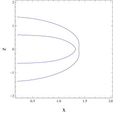
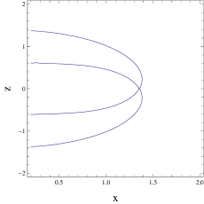
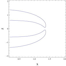
Figure 1: Shapes of the Killing horizon for $a=0.7,q=0.6$ and $M=1$ with varying values of $\epsilon$ as $0.389,0.396$ and $0.4$ (clockwise).

On the top left $\epsilon=0.389<\epsilon^{max-eq}$, the inner and outer Killing horizons have spherical topology. On the top right $\epsilon=0.396\approx\epsilon^{max-eq}$, the inner and outer Killing horizons merge at the equatorial plane. In the bottom graph $\epsilon=0.4>\epsilon^{max-eq}$, disjoint Killing horizons appear above and below the equatorial plane. Figure 2 represents the Killing horizons for negative $\epsilon$.

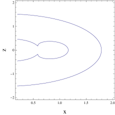
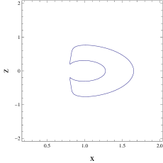
Figure 2: The Killing horizon for negative $\epsilon$. On the left $a=0.8,q=0.3,\epsilon=-0.6$ and $M=1$. On the right $a=0.96,q=0.43,\epsilon=-0.6$ and $M=1$.

In the left panel of the figure the values of the spin and charge are chosen such that $a^{2}+q^{2}<M$. Here the inner and outer Killing horizons are in the form of spherical surface. In the right panel $a^{2}+q^{2}>M$. The Killing horizon is in the shape of toroidal surface in such case.

3.2 Event horizon of the linearized charged Johannsen-Psaltis spacetime

The charged Johannsen-Psaltis metric can be treated as a small perturbation of the Kerr-Newman spacetime in terms of the deviation parameter $\epsilon$. The modifications in the Kerr-Newman metric components up to the first order in $\epsilon$ are

$$h_{tt}=-\frac{M^{3}r\left(\Sigma-2Mr+q^{2}\right)}{\Sigma^{3}},\quad h_{rr}=\frac{M^{3}r\left(\Sigma-2Mr+q^{2}\right)}{\Sigma\Delta^{2}},$$

$$h_{\theta\theta}=0,\quad h_{t\phi}=\frac{aM^{3}r\sin^{2}\theta\left(q^{2}-2Mr\right)}{\Sigma^{3}},h_{\phi\phi}=\frac{a^{2}M^{3}r\epsilon\sin^{4}\theta\left(2Mr-q^{2}+\Sigma\right)}{\Sigma^{3}}.$$ (52)

The event horizon in this case can be determined from the equation sys

$$g_{KN}^{rr}\left(1-\epsilon g_{KN}^{rr}h_{rr}\right)=0,$$ (53)

where $g_{KN}^{rr}$ is the inverse of $g_{rr}$ component of the Kerr-Newman metric and $h_{rr}$ is given in the last equation. The radius of the event horizon in this case is given by

$$r_{H}=H_{KN}\left(1+\lambda\epsilon\right),$$ (54)

where $H_{KN}$ is the event horizon of the Kerr-Newman black hole and $\lambda$ measures deviation from it. Substituting Eq. (54) in Eq. (53), and linearizing in terms of $\epsilon$, we obtain

$$\lambda=-\frac{a^{2}M^{3}\sin^{2}\theta}{2\sqrt{M^{2}-a^{2}-q^{2}}(2MH_{KN}-q^{2}-a^{2}\sin^{2}\theta)^{2}}.$$ (55)

Thus the event horizon is located at the radius

$$r_{H}=H_{KN}\left(1-\frac{\epsilon a^{2}M^{3}\sin^{2}\theta}{2\sqrt{M^{2}-a^{2}-q^{2}}(2MH_{KN}-q^{2}-a^{2}\sin^{2}\theta)^{2}}\right).$$ (56)

The Kretschmann scalar for the linearized form of (30) diverges at $r=0$, therefore, it represents a black hole.

4 Lorentz violations, closed time-like curves and regions of validity

The determinant of metric (30) is given by

$$det(g_{\mu\nu})=-\frac{\sin^{2}\theta}{64\Sigma^{2}}\Bigg{[}3a^{4}+8a^{2}r^{2}+8r^{4}+8\epsilon M^{3}r+4a^{2}(2r^{2}+a^{2})\cos 2\theta+a^{4}\cos 4\theta\Bigg{]}^{2},$$ (57)

which is independent of the charge $q$. It is negative, semi-definite and becomes zero at two values of the radii for $\epsilon<-(2Mr_{+}-q^{2})^{2}/M^{3}r_{+}$ which coincide with the location of the Killing horizon. So, the charged spacetime does not contain any Lorentz violating region.
From the $g_{\phi\phi}$ component in metric (30), we plot the closed time-like curves and combine them with the Killing horizons to show their location. These plots are shown in Figure 3. Also from $g_{\phi\phi}$ component, we can determine the upper bound for $\epsilon$ at the equatorial plane and denote it with symbol $\epsilon^{CTC}$ and is given by

$$\epsilon^{CTC}=-\frac{r^{3}\left(r^{2}\left(a^{2}+r^{2}\right)-a^{2}\left(q^{2}-2Mr\right)\right)}{a^{2}M^{3}\left(r(2M+r)-q^{2}\right)},$$ (58)

while at the equatorial plane (45) gives the value of $\epsilon$ as

$$\epsilon^{hor}=-\frac{r^{3}\left(r^{2}+a^{2}+q^{2}-2Mr\right)}{a^{2}M^{3}},$$ (59)

where symbol $\epsilon^{hor}$ shows that this is the value at the horizon for the equatorial plane. It is clear that $\epsilon^{CTC}<\epsilon^{hor}$ which leads to the result that for the equatorial plane the regions of closed time-like curves lie inside the inner Killing horizon.

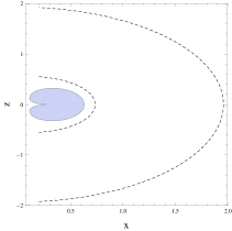
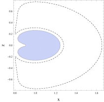
Figure 3: The Killing horizon and closed time-like curves for some values of $\epsilon,a$ and $q$. Mass $M$ has been set to 1. On the left $a=0.3,q=0.2,\epsilon=-0.3$. On the right $a=0.96,q=0.43,\epsilon=-0.6$. The dashed curves denote the inner and outer Killing horizons and the solid region shows the closed time-like curve.

In Figure 3, two cases have been plotted. In the left panel the values of $q$ and $a$ are such that $a^{2}+q^{2}<M$, resulting in an inner and outer Killing horizon and the closed time-like region lying inside the inner Killing horizon. In the right panel $a^{2}+q^{2}>M$, resulting in the toroidal shaped horizon surrounding the closed time-like region. So we conclude that the charged Johannsen-Psaltis metric does not contain closed time-like curves outside the central object.

5 Innermost stable circular orbits and the circular photon orbits

Rotation of the central object has significant effects on the motion of particles in general relativity. Consider a massive particle moving around a black hole. There exists a minimum radius at which the stable circular motion is possible. This defines the innermost stable circular orbits or the ISCO.

In this section, particle motion on the equatorial plane is considered. First the expressions for the energy and angular momentum are determined which are later employed to compute the innermost stable circular orbits and circular photon orbits.

In order to obtain the radial equation of motion, we solve the equation

$$p_{\alpha}p^{\alpha}=-m^{2},$$ (60)

for the radial momentum. Here $p_{\alpha}$ is the 4-momentum of the particle of mass $m$. The radial equation of motion, so obtained is

$$(\frac{dr}{d\tau})^{2}=R(r)=-\frac{1}{g_{rr}}(g^{tt}E^{2}+g^{\phi\phi}L^{2}-2ELg^{t\phi}+m^{2}),$$ (61)

where $\tau$ is the proper time. Here $E$ and $L$ denote the energy and angular momentum of the particle, respectively, which can be determined by solving the equations

$$R(r)=0,$$ (62)

$$\frac{dR(r)}{dr}=0.$$ (63)

This gives

$$\frac{E}{m}=\sqrt{\frac{P_{1}+P_{2}}{P_{3}}},$$ (64)

where

$$P_{1} =12a^{4}M^{3}r^{5}\epsilon\Big{(}Mr-q^{2}\Big{)}\Big{(}M^{3}\epsilon+r^{3}\Big{)}^{4}+a^{2}r^{8}\Big{(}M^{3}\epsilon+r^{3}\Big{)}^{2}\Big{[}q^{4}\Big{(}-7M^{6}\epsilon^{2}+10M^{3}r^{3}\epsilon$$

$$+8r^{6}\Big{)}+2q^{2}r\Big{(}16M^{7}\epsilon^{2}-9M^{6}r\epsilon^{2}-16M^{4}r^{3}\epsilon+6M^{3}r^{4}\epsilon-14Mr^{6}+6r^{7}\Big{)}$$

$$+Mr^{2}\Big{(}-40M^{7}\epsilon^{2}+48M^{6}r\epsilon^{2}-15M^{5}r^{2}\epsilon^{2}+16M^{4}r^{3}\epsilon-6M^{2}r^{5}\epsilon+20Mr^{6}-12r^{7}\Big{)}\Big{]},$$ (65)

$$P_{2} =2\Big{[}2\Big{(}r^{26}\mp P_{4}\Big{)}-48M^{12}r^{14}\epsilon^{3}+68M^{11}r^{15}\epsilon^{3}-32M^{10}r^{16}\epsilon^{3}+5M^{9}r^{17}(\epsilon-24)\epsilon^{2}$$

$$+168M^{8}r^{18}\epsilon^{2}-78M^{7}r^{19}\epsilon^{2}+12M^{6}r^{20}(\epsilon-8)\epsilon+132M^{5}r^{21}\epsilon-60M^{4}r^{22}\epsilon$$

$$+q^{6}r^{11}\Big{(}M^{3}\epsilon+r^{3}\Big{)}^{2}\Big{(}7M^{3}\epsilon+4r^{3}\Big{)}-3M^{3}r^{23}(8-3\epsilon)+32M^{2}r^{24}$$

$$-q^{4}r^{12}\Big{(}M^{3}\epsilon+r^{3}\Big{)}^{2}\Big{(}40M^{4}\epsilon-19M^{3}r\epsilon+22Mr^{3}-10r^{4}\Big{)}$$

$$+q^{2}r^{13}(2M-r)\Big{(}M^{3}\epsilon+r^{3}\Big{)}^{2}\Big{(}38M^{4}\epsilon-17M^{3}r\epsilon+20Mr^{3}-8r^{4}\Big{)}-14Mr^{25}\Big{]},$$ (66)

$$P_{3} =r^{13}\Big{[}8a^{2}\Big{(}q^{2}-Mr\Big{)}\Big{(}M^{3}\epsilon+r^{3}\Big{)}^{2}\Big{(}5M^{3}\epsilon+2r^{3}\Big{)}+r^{3}\Big{(}q^{2}\Big{(}7M^{3}\epsilon+4r^{3}\Big{)}$$

$$+r\Big{(}-12M^{4}\epsilon+5M^{3}r\epsilon-6Mr^{3}+2r^{4}\Big{)}\Big{)}^{2}\Big{]},$$ (67)

$$P_{4} =\Big{[}a^{2}r^{10}\Big{(}q^{2}-Mr\Big{)}^{2}\Big{(}M^{3}\epsilon+r^{3}\Big{)}^{6}\Big{(}a^{2}\Big{(}M^{3}\epsilon+r^{3}\Big{)}+r^{3}\Big{(}-2Mr+q^{2}+r^{2}\Big{)}\Big{)}^{2}\Big{(}9a^{2}M^{6}\epsilon^{2}$$

$$+16M^{4}r^{4}\epsilon-2q^{2}\Big{(}5M^{3}r^{3}\epsilon+2r^{6}\Big{)}-6M^{3}r^{5}\epsilon+4Mr^{7}\Big{)}\Big{]}^{\frac{1}{2}}.$$ (68)

The angular momentum is

$$\frac{L}{m} =\pm\frac{1}{\sqrt{P_{3}}\beta}\Bigg{[}\Big{(}\mp 2a^{2}r^{6}(q^{6}+q^{2}r^{2}M(8M-5r)+rq^{4}(2r-5M)$$

$$+M^{2}r^{3}(3r-4M))(r^{3}+\epsilon M^{3})^{4}+a^{4}r^{3}(q^{2}-Mr)(r^{3}+\epsilon M^{3})^{4}(2Mr^{4}-4M^{4}r\epsilon$$

$$+q^{2}(-2r^{3}+M^{3}\epsilon))+P_{4}\Big{)}\sqrt{P_{1}+P_{2}}\Bigg{]}.$$ (69)

where

$$\beta =ar^{3}(Mr-q^{2})(M^{3}\epsilon+r^{3})^{4}[2r^{3}\left(r(r-2M)+q^{2}\right)^{2}+a^{2}(q^{2}(2r^{3}-M^{3}\epsilon)$$

$$+Mr(4M^{3}\epsilon-3M^{2}r\epsilon-2r^{3}))].$$ (70)

Here the upper sign indicates that the particle corotates with the black hole while the lower sign refers to the opposite situation.

In the case $\epsilon=0$, the above expressions for the energy and angular momentum reduce to the ones obtained for the Kerr-Newman metric dp

$$\frac{E}{m}=\frac{r^{2}-2Mr+q^{2}\pm a(Mr-q^{2})^{1/2}}{r\sqrt{(r^{2}-3Mr+2q^{2}\pm 2a(Mr-q^{2})^{1/2})}},$$ (71)

$$\frac{L}{m}=\pm\frac{(Mr-q^{2})^{1/2}(r^{2}+a^{2}\mp 2a(Mr-q^{2})^{1/2})\mp aq^{2}}{r\sqrt{(r^{2}-3Mr+2q^{2}\pm 2a(Mr-q^{2})^{1/2})}}.$$ (72)

Taking $q=0=\epsilon$ gives the energy and angular momentum for the Kerr metric bar

$$\frac{E}{m}=\frac{r^{3/2}-2Mr^{1/2}\pm aM^{1/2}}{r^{3/4}\sqrt{r^{3/2}-3Mr^{1/2}\pm 2aM^{1/2}}},$$ (73)

$$\frac{L}{m}=\pm\frac{M^{1/2}(r^{2}\mp 2aM^{1/2}r^{1/2}+a^{2})}{r^{3/4}\sqrt{r^{3/2}-3Mr^{1/2}\pm 2aM^{1/2}}}.$$ (74)

The ISCO is determined by numerically solving the equation

$$\frac{dE}{dr}=0.$$ (75)

In Figure 4, radial dependence of ISCO is shown for some particular values of the parameters.

Figure 4: The Inner most stable circular orbits for some values of $\epsilon,a$ and $q$. Mass $M$ has been set to 1. On the left $a=0.6$ with varying values of charge $q$. Starting from the upper curve, the values of $\epsilon$ are $-1,1,2$ respectively. On the right $q=0.4$ with varying values of the rotation parameter. Starting from the upper curve, the values of $\epsilon$ are $-2,-1,2$ respectively.

The circualr photon orbits are located where

$$\frac{E}{m}\rightarrow\infty,\quad\frac{L}{m}\rightarrow\infty.$$ (76)

In Figure 5, radial profile of the circular photon orbit is shown.

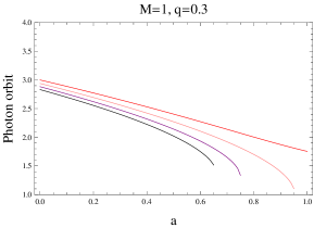
Figure 5: The circular photon orbits for some values of $\epsilon$ and $a$. Mass $M$ has been set to 1 and $q$ is taken as $q=0.3$. Red plot is for $\epsilon=-1$, pink for $\epsilon=0$, purple for $\epsilon=1$, and black for $\epsilon=2$.

As in the ISCO case, increasing the value of the deformation parameter decreases the radius of the photon orbits.

6 Summary and conclusion

Many modified theories of gravity have been developed that lead to spacetimes that are different from Kerr’s in that they have parameters other than mass and spin. If one sets all the deviations back to zero, such spacetimes reduce to Kerr.

One such spacetime has been formulated by Johannsen and Psaltis jp . This metric takes the deformed Schwarzschild spacetime as the starting point and applies Newman-Janis algorithm to obtain a rotating spacetime. In this paper we have extended the approach to obtain the charged analogue of the Johannsen-Psaltis metric. This has been done by taking the Reissner-Nordström spacetime as the seed metric and applying Newman-Janis algorithm to it. This leads to a spacetime which is stationary, axisymmetric and asymptotically flat. It gives the Johannsen-Psaltis metric on setting charge equal to zero. Setting the deviation parameter $\epsilon=0$ yields the Kerr-Newman metric. The electromagnetic 4-potential contains the deviation parameter $\epsilon$ in its radial component, thus inducing $\theta$ dependence in it. Thus $A_{r}$ component cannot be gauged away so we have a nonzero $A_{r}$ making the 4-potential $A_{\mu}$ different from the case of Kerr-Newman. Further analysis of $A_{r}$ revels that it depends on the mass $M$ through the deviation parameter $\epsilon$ which we can consider as a coupling between the gravitational and the electromagnetic fields.

The event horizon of the charged Johannsen-Psaltis spacetime has been studied. Here horizon is taken as a general function sys of $\theta$, $H(\theta)$, so that horizon is $r=H(\theta)$. The equation which determines $H(\theta)$ is given by (38). Next, the Killing horizon is discussed. The graphs are drawn for different values of parameters $a,q,M,\epsilon$. The graphs show that for $\epsilon<\epsilon^{max-pole}$, the inner and outer horizons have spherical topology while for $\epsilon\approx\epsilon^{max-pole}$ Killing horizons intersect at the equatorial plane. In case of $\epsilon>\epsilon^{max-pole}$, disjoint Killing horizons appear above and below the equatorial plane. For negative $\epsilon$, the inner and outer Killing horizons are in the shape of the spherical surface for $a^{2}+q^{2}<M$ while the shape changes to a toroidal surface if $a^{2}+q^{2}>M$. From the determinant of the charged Johannsen-Psaltis metric we find that it is independent of the Lorentz violating regions. The plots of the closed time-like curve and the Killing horizons show that it is surrounded by the Killing horizon. Therefore, the charged Johannsen-Psaltis metric does not contain closed time-like curves outside of the central body.

Considering the charged Johannsen-Psaltis metric as a perturbation of the Kerr-Newman metric upto the first order in $\epsilon$, we find that its Kretschmann scalar diverges at $r=0$, therefore it represents a black hole for all values of $\epsilon$.

The analysis of the ISCO and circular photon orbits shows the dependence on $\epsilon$. Both show decreasing behavior with the increase of $\epsilon$.

- (1) W. J. van Stockum, Proc. R. Soc. Edinburgh 57 (1937) 135.
- (2) W. Israel, Phys. Rev. 164 (1967) 1776; W. Israel, Commun. Math. Phys. 8 (1968) 245; B. Carter, Phys. Rev. Lett. 26 (1971) 331; S. W. Hawking, Commun. Math. Phys. 25 (1972) 152; D. C. Robinson, Phys. Rev. Lett. 34 (1975) 905.
- (3) E. T. Newman and A. I. Janis, J. Math. Phys. 6 (1965) 915.
- (4) L. Herrera and J. Jiménez, J. Math. Phys. 23 (1982) 2339; S. Viaggiu, Int. J. Mod. Phys. D 15 (2006) 1441.
- (5) E. T. Newman, E. Couch, K. Chinnapared, A. Exton, A. Prakash and R. Torrence, J. Math. Phys. 6 (1965) 918.
- (6) S. A. Hughes, Probing strong-field gravity and black holes with gravitational waves, arXiv:1002.2591 (2010); T. Johannsen and D. Psaltis, ApJ. 716 (2010) 187; N. Wex and S. M. Kopeikin, ApJ. 514 (1999) 388.
- (7) C. M. Will, Theory and experiment in gravitational physics, Cambridge University Press, Cambridge (1993).
- (8) S. J. Vigeland, N. Yunes and L. C. Stein, Phys. Rev. D 83 (2011) 104027.
- (9) T. Johannsen and D. Psaltis, Phys. Rev. D 83 (2011) 124015.
- (10) N. Yunes and F. Pretorius, Phys. Rev. D 79 (2009) 084043.
- (11) D. Hansen and N. Yunes, Phys. Rev. D 88 (2013) 104020.
- (12) S. J. Vigeland and S. A. Hughes, Phys. Rev. D 81(2010) 024030; S. J. Vigeland, N. Yunes and L. Stein, Phys. Rev. D 83 (2011) 104027.
- (13) F. Filippini and G. Tasinato, JCAP 01 (2018) 033.
- (14) S. Chen and J. Jing, Phys. Rev. D 89 (2014) 104014.
- (15) E. T. Newman and R. Penrose, J. Math. Phys. 3 (1962) 566.
- (16) F. Caravelli and L. Modesto, Classical Quantum Gravity 27 (2010) 245022.
- (17) T. Johannsen, Phys. Rev. D 87 (2013) 124017.
- (18) N. Dadhich and P. P. Kale, J. Math. Phys. 18 (1977) 1727.
- (19) J. M. Bardeen in Black holes, Gordon and Breach, New York (1973).