Multi-Agent Reinforcement Learning Based Resource Allocation for UAV Networks

Abstract

Unmanned aerial vehicles (UAVs) are capable of serving as aerial base stations (BSs) for providing both cost-effective and on-demand wireless communications. This article investigates dynamic resource allocation of multiple UAVs enabled communication networks with the goal of maximizing long-term rewards. More particularly, each UAV communicates with a ground user by automatically selecting its communicating users, power levels and subchannels without any information exchange among UAVs. To model the uncertainty of environments, we formulate the long-term resource allocation problem as a stochastic game for maximizing the expected rewards, where each UAV becomes a learning agent and each resource allocation solution corresponds to an action taken by the UAVs. Afterwards, we develop a multi-agent reinforcement learning (MARL) framework that each agent discovers its best strategy according to its local observations using learning. More specifically, we propose an agent-independent method, for which all agents conduct a decision algorithm independently but share a common structure based on Q-learning. Finally, simulation results reveal that: 1) appropriate parameters for exploitation and exploration are capable of enhancing the performance of the proposed MARL based resource allocation algorithm; 2) the proposed MARL algorithm provides acceptable performance compared to the case with complete information exchanges among UAVs. By doing so, it strikes a good tradeoff between performance gains and information exchange overheads.

I Introduction

Aerial communication networks, encouraging new innovative functions to deploy wireless infrastructure, have recently attracted increasing interests for providing high network capacity and enhancing coverage [1]. Unmanned aerial vehicles (UAVs), also known as remotely piloted aircraft systems (RPAS) or drones, are small pilotless aircraft that are rapidly deployable for complementing terrestrial communications based on the 3rd Generation Partnership Project (3GPP) LTE-A (Long term evolution-advanced) [2]. In contrast to channel characteristics of terrestrial communications, the channels of UAV-to-ground communications are more probably line-of-sight (LoS) links [3], which is beneficial for wireless communications.

In particular, UAVs based different aerial platforms that for providing wireless services have attracted extensive research and industry efforts in terms of the issues of deployment, navigation and control [4]. Nevertheless, resource allocation such as transmit power, serving users and subchannels, as a key communication problem, is also essential to further enhance the energy-efficiency and coverage for UAV-enabled communication networks.

I-A Prior Works

Compared to terrestrial BSs, UAVs are generally faster to deploy and more flexible to configure. The deployment of UAVs in terms of altitude and distance between UAVs was investigated for UAV-enabled small cells in [5]. In [6], a three-dimensional (3D) deployment algorithm based on circle packing is developed for maximizing the downlink coverage performance. Additionaly, a 3D deployment algorithm of a single UAV is developed for maximizing the number of covered users in [7]. Moreover, by fixing the altitudes, a successive UAV placement approach was proposed to minimize the number of UAVs required while guaranteeing each ground user to be covered by at least one UAV in [8].

Despite the deployment optimization of UAVs, trajectory designs of UAVs for optimizing the communication performance have attracted tremendous attentions, such as in [9, 10, 11]. In [9], the authors considered one UAV as a mobile relay and investigated the throughput maximization problem by optimizing power allocation and the UAV’s trajectory. Then, a designing approach of the UAV’s trajectory based on successive convex approximation (SCA) techniques was proposed in [9]. By transforming the continuous trajectory into a set of discrete waypoints, the authors in [10] investigated the UAV’s trajectory design with minimizing the mission completion time in a UAV-enabled multicasting system. Additionally, multiple-UAV enabled wireless communication networks (multi-UAV networks) were considered in [11], where a joint design for optimizing trajectory and resource allocation was studied with the goal of guaranteeing fairness by maximizing the minimum throughput among users. In [12], the authors proposed a joint of subchannel assignment and trajectory design approach to strike a tardeoff between the sum rate and the delay of sensing tasks for a multi-UAV aided uplink single cell network.

Due to the versatility and manoeuvrability of UAVs, human intervention becomes restricted for UAVs’ control design. Therefore, machine learning based intelligent control of UAVs is desired for enhancing the performance for UAV-enabled communication networks. Neuro network based trajectory designs were considered from the perspective of UAVs’ manufactured structures in [13] and [14]. Regarding UAVs enabled communication networks, a weighted expectation based predictive on-demand deployment approach of UAVs was proposed to minimize the transmit power in [15], where Gaussian mixture model was used for building data distributions. In [16], the authors studied the autonomous path planning of UAVs by jointly taking energy efficiency, lantency and interference into consideration, in which a echo state network based deep reinforement learning algorithm was proposed. In [17], the authors proposed a liquid state machine (LSM) based resource allocation algorithm for cache enabled UAVs over LTE licensed and unlicensed bands. Additionally, a log-linear learning based joint channel-slot selection algorithm was developed for multi-UAV networks in [18].

I-B Motivation and Contributions

As discussed above, machine learning is a promising and power tool to provide autonomous and effective solutions in an intelligent manner to enhance the UAV-enabled communication networks. However, most research contributions focus on the deployment and trajectory designs of UAVs in communication networks, such as [15, 16, 17]. Though resource allocation schemes such as transmit power and subchannels were considered for UAV-enabled communication networks in [11] and [12], the prior studies focused on time-independent scenarios. That is the optimization design is independent for each time slot. Moreover, for time-dependent scenarios, [17] and [18] investigated the potentials of machine learning based resource allocation algorithms. However, most of the proposed machine learning algorithms mainly focused on single UAV scenarios or multi-UAV scenarios by assuming the availability of complete network information for each UAV. In practice, it is non-trivial to obtain perfect knowledge of dynamic environments due to the high movement speed of UAVs [19, 20], which imposes formidable challenges on the design of reliable UAV-enabled wireless communications. Besides, most existing research contributions focus on centralized approaches, which makes modeling and computational tasks become challenging as the network size continues to increase. Multi-agent reinforcement learning (MARL) is capable of providing a distributed perspective on the intelligent resource management for UAV-enabled communication networks especially when these UAVs only have individual local information.

The main benefits of MARL are: 1) agents consider individual application-specific nature and environment; 2) local exchanges between agents can be modeled and investigated; 3) difficulties in modelling and computation can be handled in distributed manners. The applications of MARL for cognitive radio networks were studied in [21] and [22]. Specifically, in [21], the authors focused on the feasibilities of MARL based channel selection algorithms for a specific scenario with two secondary users. A real-time aggregated interference scheme based on MARL was investigated in [22] for wireless regional area networks (WRANs). Moreover, in [23], the authors proposed a MARL based channel and power level selection algorithm for device-to-device (D2D) pairs in heterogeneous cellular networks. The potential of machine learning based user clustering for mmWave-NOMA networks was presented in [24]. Therefore, invoking MARL to UAV-enabled communication networks provides a promising solution for intelligent resource management. Due to the high mobility and adaptive altitude, to the best of our knowledge, multi-UAV networks are not well-investigated, especially for the resource allocation from the perspective of MARL. However, it is challenging for MARL based multi-UAV networks to specify a suitable objective and strike a exploration-exploitation tradeoff.

Motivated by the features of MARL and UAVs, this article aims to develop a MARL framework for multi-UAV networks. More specifically, we consider a multi-UAV enabled downlink wireless network, in which multiple UAVs try to communicate with ground users simultaneously. Each UAV flies according to the predefined trajectory. It is assumed that all UAVs communicate with ground users without the assistance of a central controller. Hence, each UAV can only observe its local information. Based on the proposed framework, our major contributions are summarized as follows:

1. We investigate the optimization problem of maximizing long-term rewards of multi-UAV downlink networks by jointly designing user, power level and subchannel selection strategies. Specifically, we formulate a quality of service (QoS) constrained energy efficiency function as the reward function for providing a reliable communication. Because of the time-dependent nature and environment uncertainties, the formulated optimization problem is non-trivial. To solve the challenging problem, we propose a learning based dynamic resource allocation algorithm.

2. We propose a novel framework based on stochastic game theory [25] to model the dynamic resource allocation problem of multi-UAV networks, in which each UAV becomes a learning agent and each resource allocation solution corresponds to an action taken by the UAVs. Particularly, in the formulated stochastic game, the actions for each UAV satisfy the properties of Markov chain [26], that is the reward of a UAV is only dependant on the current state and action. Furthermore, this framework can be also applied to model the resource allocation problem for a wide range of dynamic multi-UAV systems.

3. We develop a MARL based resource allocation algorithm for solving the formulated stochastic game of multi-UAV networks. Specifically, each UAV as an independent learning agent runs a standard Q-learning algorithm by ignoring the other UAVs, and hence information exchanges between UAVs and computational burdens on each UAV are substantially reduced. Additionally, we also provide a convergence proof of the proposed MARL based resource allocation algorithm.

4. Simulation results are provided to derive parameters for exploitation and exploration in the $\epsilon$-greedy method over different network setups. Moreover, simulation results also demonstrate that the proposed MARL based resource allocation framework for multi-UAV networks strikes a good tradeoff between performance gains and information exchange overheads.

I-C Organization

The rest of this article is organized as follows. In Section II, the system model for downlink multi-UAV networks is presented. The problem of resource allocation is formulated and a stochastic game framework for the considered multi-UAV network is presented in Section III. In Section IV, a Q-learning based MARL algorithm for resource allocation is designed. Simulation results are presented in Section V, which is followed by the conclusions in Section VI.

II System Model

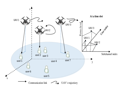
Figure 1: Illustration of multi-UAV communication networks.

Consider a multi-UAV downlink communication network as illustrated in Fig. 1 operating in a discrete-time axis, which consists of $M$ single-antenna UAVs and $L$ single-antenna users, denoted by $\mathcal{M}=\{1,\cdots,M\}$ and $\mathcal{L}=\{1,\cdots,L\}$, respectively. The ground users are randomly distributed in the considered disk with radius $r_{d}$. As shown in Fig. 1, multiple UAVs fly over this region and communicate with ground users by providing direct communication connectivity from the sky [1]. The total bandwidth $W$ that the UAVs can operate is divided into $K$ orthogonal subchannels, denoted by $\mathcal{K}=\{1,\cdots,K\}$. Note that the subchannels occupied by UAVs may overlap with each other. Moreover, it is assumed that UAVs fly autonomously without human intervention based on pre-programmed flight plans as in [27]. That is the trajectories of UAVs are predefined based on the pre-programmed flight plans. As shown in Fig. 1, there are three UAVs flying on the considered region based on the pre-defined trajectories, respectively. This article focuses on the dynamic design of resource allocation for multi-UAV networks in term of user, power level and subchannel selections. Additionally, assuming that all UAVs communicate without the assistance of a central controller and have no global knowledge of wireless communication environments. In other words, the channel state information (CSI) between a UAV and users are known locally. This assumption is reasonable in practical due to the mobilities of UAVs, which is similar to the research contributions [19, 20].

II-A UAV-to-Ground Channel Model

In contrast to the propagation of terrestrial communications, the air-to-ground (A2G) channel is highly dependent on the altitude, elevation angle and the type of the propagation environment [3, 4, 2]. In this article, we investigate the dynamic resource allocation problem for multi-UAV networks under two types of UAV-to-ground channel models:

II-A1 Probabilistic Model

As discussed in [3, 2], UAV-to-ground communication links can be modeled by a probabilistic path loss model, in which the LoS and non-LoS (NLoS) links can be considered separately with different probabilities of occurrences. According to [3], at time slot $t$, the probability of having a LoS connection between UAV $m$ and a ground user $l$ is given by

$$P^{\mathrm{LoS}}(t)=\frac{1}{1+\mathfrak{a}\exp(-\mathfrak{b}\sin^{-1}(\frac{H}{d_{m,l}(t)})-\mathfrak{a})},$$ (1)

where $\mathfrak{a}$ and $\mathfrak{b}$ are constants that depend on the environment. $d_{m,l}$ denotes the distance between UAV $m$ and user $l$ and $H$ denotes the altitude of UAV $m$. Furthermore, the probability of have NLoS links is $P^{\mathrm{NLoS}}(t)=1-P^{\mathrm{LoS}}(t)$.

Accordingly, in time slot $t$, the LoS and NLoS pathloss from UAV $m$ to the ground user $l$ can be expressed as

$$PL_{m,l}^{\mathrm{LoS}} =L^{\mathrm{FS}}_{m,l}(t)+\eta^{\mathrm{LoS}},$$ (2a)

$$PL_{m,l}^{\mathrm{NLoS}} =L^{\mathrm{FS}}_{m,l}(t)+\eta^{\mathrm{NLoS}},$$ (2b)

where $L^{\mathrm{FS}}_{m,l}(t)$ denotes the free space pathloss with $L^{\mathrm{FS}}_{m,l}(t)=20\log(d_{m,l}(t))+20\log(f)+20\log(\frac{4\pi}{c})$, and $f$ is the carrier frequency. Furthermore, $\eta^{\mathrm{LoS}}$ and $\eta^{\mathrm{NLoS}}$ are the mean additional losses for LoS and NLoS, respectively. Therefore, at time slot $t$, the average pathloss between UAV $m$ and user $l$ can be expressed as

$$L_{m,l}(t)=P^{\mathrm{LoS}}(t)\cdot PL_{m,l}^{\mathrm{LoS}}(t)+P^{\mathrm{NLoS}}(t)\cdot PL_{m,l}^{\mathrm{NLoS}}(t).$$ (3)

II-A2 LoS Model

As discussed in [9], the LoS model provides a good approximation for practical UAV-to-ground communications. In the LoS model, the path loss between a UAV and a ground user relies on the locations of the UAV and the ground user as well as the type of propagation. Specifically, under the LoS model, the channel gains between the UAVs and the users follow the free space path loss model, which is determined by the distance between the UAV and the user. Therefore, at time slot $t$, the LoS channel power gain from the $m$-th UAV to the $l$-th ground user can be expressed as

$$g_{m,l}(t)=\beta_{0}d_{m,l}^{-\alpha}(t)=\frac{\beta_{0}}{\big{(}\|\mathbf{v}_{l}-\mathbf{u}_{m}(t)\|^{2}+H_{m}^{2}\big{)}^{\frac{\alpha}{2}}},$$ (4)

where $\mathbf{u}_{m}(t)=(x_{m}(t),y_{m}(t))$, and $(x_{m}(t),y_{m}(t))$ denotes the location of UAV $m$ in the horizontal dimension at time slot $t$. Correspondingly, $\mathbf{v}_{l}=(x_{l},y_{l})$ denotes the location of user $l$. Furthermore, $\beta_{0}$ denotes the channel power gain at the reference distance of $d_{0}=1$ m, and $\alpha\geq 2$ is the path loss exponent.

II-B Signal Model

In the UAV-to-ground transmission, the interference to each UAV-to-ground user pair is created by other UAVs operating on the same subchannel. Let $c_{m}^{k}(t)$ denote the indicator of subchannel, where $c_{m}^{k}(t)=1$ if subchannel $k$ occupied by UAV $m$ at time slot $t$; $c_{m}^{k}(t)=0$, otherwise. It satisfies

$$\sum_{k\in\mathcal{K}}c_{m}^{k}(t)\leq 1.$$ (5)

That is each UAV can only occupy a single subchannel for each time slot. Let $a_{m}^{l}(t)$ be the indicator of users. $a_{m}^{l}(t)=1$ if user $l$ served by UAV $m$ in time slot $t$; $a_{m}^{l}(t)=0$, otherwise. Therefore, the observed signal-to-interference-plus-noise ratio (SINR) for a UAV-to-ground user communication between UAV $m$ and user $l$ over subchannel $k$ at time slot $t$ is given by

$$\gamma_{m,l}^{k}(t)=\frac{G_{m,l}^{k}(t)a_{m}^{l}(t)c_{m}^{k}(t)P_{m}(t)}{I_{m,l}^{k}(t)+\sigma^{2}},$$ (6)

where $G_{m,l}^{k}(t)$ denotes the channel gain between UAV $m$ and user $l$ over subchannel $k$ at time slot $t$. $P_{m}(t)$ denotes the transmit power selected by UAV $m$ at time slot $t$. $I_{m,l}^{k}(t)$ is the interference to UAV $m$ with $I_{m,l}^{k}(t)=\sum_{j\in\mathcal{M},j\neq m}G_{j,l}^{k}(t)c_{m}^{k}(t)P_{j}(t)$. Therefore, at any time slot $t$, the SINR for UAV $m$ can be expressed as

$$\gamma_{m}(t)=\sum_{l\in\mathcal{L}}\sum_{k\in\mathcal{K}}\gamma_{m,l}^{k}(t).$$ (7)

In this article, discrete transmit power control is adopted at UAVs [28]. The transmit power values by each UAV to communicate with its respective connected user can be expressed as a vector $\mathbf{P}=\{P_{1},\cdots,P_{J}\}$. For each UAV $m$, we define a binary variable $p_{m}^{j}(t)$, $j\in\mathcal{J}=\{1,\cdots,J\}$. $p_{m}^{j}(t)=1$, if UAV $m$ selects to transmit at a power level $P_{j}$ at time slot $t$; and $p_{m}^{j}(t)=0$, otherwise. Note that only one power level can be selected at each time slot $t$ by UAV $m$, we have

$$\sum_{j\in\mathcal{J}}p_{m}^{j}(t)\leq 1,\forall m\in\mathcal{M}.$$ (8)

As a result, we can define a finite set of possible power level selection decisions made by UAV $m$, as follows.

$$\mathcal{P}_{m}=\{p_{m}(t)\in\mathbf{P}|\sum_{j\in\mathcal{J}}p_{m}^{j}(t)\leq 1\},~{}\forall m\in\mathcal{M}.$$ (9)

Similarly, we also define finite sets of all possible subchannel selection and user selection by UAV $m$, respectively, which are given as follows:

$$\mathcal{C}_{m}= \{c_{m}(t)\in\mathcal{K}|\sum_{k\in\mathcal{K}}c_{m}^{k}(t)\leq 1\},\forall m\in\mathcal{M},$$ (10)

$$\mathcal{A}_{m}= \{a_{m}(t)\in\mathcal{L}|\sum_{l\in\mathcal{L}}a_{m}^{l}(t)\leq 1\},\forall m\in\mathcal{M}.$$ (11)

To proceed further, we assume that the considered multi-UAV network operates on a discrete-time basis where the time axis is partitioned into equal non-overlapping time intervals (slots). Furthermore, the communication parameters are assumed to remain constant during each time slot. Let $t$ denote an integer valued time slot index. Particularly, each UAV holds the CSI of all ground users and decisions for a fixed time interval $T_{s}\geq 1$ slots, which is called decision period. We consider the following scheduling strategy for the transmissions of UAVs: Any UAV is assigned a time slot $t$ to start its transmission and must finish its transmission and select the new strategy or reselect the old strategy by the end of its decision period, i.e., at slot $t+T_{s}$. We also assume that the UAVs do not know the accurate duration of their stay in the network. This feature motivates us to design an on-line learning algorithm for optimizing the long-term energy-efficiency performance of multi-UAV networks.

III Stochastic Game Framework for Multi-UAV Networks

In this section, we first describe the optimization problem investigated in this article. Then, to model the uncertainty of stochastic environments, we formulate the problem of joint user, power level and subchannel selections by UAVs to be a stochastic game.

III-A Problem Formulation

Note that from (6) to achieve the maximal throughput, each UAV transmits at a maximal power level, which, in turn, results in increasing interference to other UAVs. Hence, to provide reliable communications of UAVs, the main goal of the dynamic design for joint user, power level and subchannel selection is to ensure that the SINRs provided by the UAVs no less than the predefined thresholds. Specifically, the mathematical form can be expressed as

$$\gamma_{m}(t)\geq\bar{\gamma},\forall m\in\mathcal{M},$$ (12)

where $\bar{\gamma}$ denotes the targeted QoS threshold of users served by UAVs. At time slot $t$, if the constraint (12) is satisfied, then the UAV obtains a reward $R_{m}(t)$, defined as the difference between the throughput and the cost of power consumption achieved by the selected user, subchannel and power level. Otherwise, it receives a zero reward. Therefore, we can express the reward function $R_{m}(t)$ of UAV $m$ at time slot $t$, as follows:

$$R_{m}(t)=\begin{cases}\frac{W}{K}\log(1+\gamma_{m}(t))-\omega_{m}P_{m}(t),&\text{if}~{}\gamma_{m}(t)\geq\bar{\gamma}_{m},\\ 0,&\text{o.w.},\end{cases}$$ (13)

for all $m\in\mathcal{M}$ and the corresponding immediate reward is denoted as $R_{m}(t)$. In (13), $\omega_{m}$ is the cost per unit level of power. Note that at any time slot $t$, the instantaneous reward of UAV $m$ in (13) relies on: 1) the observed information: the individual user, subchannel and power level decisions of UAV $m$, i.e., $a_{m}(t)$, $c_{m}(t)$ and $p_{m}(t)$. In addition, it also relates with the current channel gain $G_{m,l}^{k}(t)$; 2) unobserved information: the subchannels and power levels selected by other UAVs and the channel gains. It should be pointed out that we omitted the fixed power consumption for UAVs, such as the power consumed by controller units and data processing [29].

Next, we consider to maximize the long-term reward $v_{m}(t)$ by selecting the served user, subchannel and transmit power level at each time slot. Particularly, we adopt a future discounted reward [30] as the measurement for each UAV. Specifically, at a certain time slot of the process, the discounted reward is the sum of its payoff in the present time slot, plus the sum of future rewards discounted by a constant factor. Therefore, the considered long-term reward of UAV $m$ is given by

$$v_{m}(t)=\sum_{\tau=0}^{+\infty}\delta^{\tau}R_{m}(t+\tau+1),$$ (14)

where $\delta$ denotes the discount factor with $0\leq\delta<1$. Specifically, values of $\delta$ reflect the effect of future rewards on the optimal decisions: if $\delta$ is close to 0, it means that the decision emphasizes the near-term gain; By contrast, if $\delta$ is close to 1, it gives more weights to future rewards and we say the decisions are farsighted.

Next we introduce the set of all possible user, subchannel and power level decisions made by UAV $m$, $m\in\mathcal{M}$, which can be denoted as $\Theta_{m}=\mathcal{A}_{m}\otimes\mathcal{C}_{m}\otimes\mathcal{P}_{m}$ with $\otimes$ denoting the Cartesian product. Consequently, the objective of each UAV $m$ is to make a selection $\theta_{m}^{*}(t)=(a_{m}^{*}(t),c_{m}^{*}(t),p_{m}^{*}(t))\in\Theta_{m}$, which maximizes its long-term reward in (14). Hence the optimization problem for UAV $m$, $m\in\mathcal{M}$, can be formulated as

$$\theta_{m}^{*}(t)={\mathrm{arg}\max}_{\theta_{m}\in\Theta_{m}}R_{m}(t).$$ (15)

Note that the optimization design for the considered multi-UAV network consists of $M$ subproblems, which corresponds to $M$ different UAVs. Moreover, each UAV has no information about other UAVs such as their rewards, hence one cannot solve problem (15) accurately. To solve the optimization problem (15) in stochastic environments, we try to formulate the problem of joint user, subchannel and power level selections by UAVs to a stochastic non-cooperative game in the following subsection.

III-B Stochastic Game Formulation

In this subsection, we consider to model the formulated problem (15) by adopting a stochastic game (also called Markov game) framework [25], since it is the generalization of the Markov decision processes to the multi-agent case.

In the considered network, $M$ UAVs communicate to users with having no information about the operating environment. It is assumed that all UAVs are selfish and rational. Hence, at any time slot $t$, all UAVs select their actions non-cooperatively to maximize the long-term rewards in (15). Note that the action for each UAV $m$ is selected from its action space $\Theta_{m}$. The action conducted by UAV $m$ at time slot $t$, is a triple $\theta_{m}(t)=(a_{m}(t),c_{m}(t),p_{m}(t))\in\Theta_{m}$, where $a_{m}(t),~{}c_{m}(t)$ and $p_{m}(t)$ represent the selected user, subchannel and power level respectively, for UAV $m$ at time slot $t$. For each UAV $m$, denote by $\theta_{-m}(t)$ the actions conducted by the other $M-1$ UAVs at time slot $t$, i.e., $\theta_{-m}(t)\in\Theta\setminus\Theta_{m}$.

As a result, the instantaneous SINR of UAV $m$ at time slot $t$ can be rewritten as

$$\begin{aligned} \gamma_{m}(t)[\theta_{m}(t),\theta_{-m}(t),\mathbf{G}_{m}(t)]=\sum_{l\in\mathcal{L}}\sum_{k\in\mathcal{K}}\frac{S_{m,l}^{k}(t)[\theta_{m}(t),\theta_{-m}(t),\mathbf{G}_{m,l}(t)]}{I_{m,l}^{k}(t)[\theta_{m}(t),\theta_{-m}(t),\mathbf{G}_{m,l}(t)]+\sigma^{2}},\end{aligned}$$ (16)

where $S_{m,l}^{k}(t)=G_{m,l}^{k}(t)a_{m}^{l}(t)c_{m}^{k}(t)P_{m}(t)$, and $I_{m,l}^{k}(t)(\cdot)$ is given in (6). Furthermore, $\mathbf{G}_{m,l}(t)$ denotes the matrix of instantaneous channel responses between UAV $m$ and user $l$ at time slot $t$, which can be expressed as

$$\mathbf{G}_{m,l}(t)=\begin{bmatrix}G_{1,l}^{1}(t)&\cdots&G_{1,l}^{K}(t)\\ \vdots&\ddots&\vdots\\ G_{M,l}^{1}(t)&\cdots&G_{M,l}^{K}(t)\end{bmatrix},$$ (17)

with $\mathbf{G}_{m,l}(t)\in\mathbb{R}^{M\times K}$, for all $l\in\mathcal{L}$ and $m\in\mathcal{M}$.

At any time slot $t$, each UAV $m$ can measure its current SINR level $\gamma_{m}(t)$. Hence, the sate $s_{m}(t)$ for each UAV $m$, $m\in\mathcal{M}$, is fully observed, which can be defined as

$$s_{m}(t)=\begin{cases}1,&\text{if}~{}\gamma_{m}(t)\geq\bar{\gamma},\\ 0,&\text{o.w.}.\end{cases}$$ (18)

Let $\mathbf{s}=(s_{1},\cdots,s_{M})$ be a state vector for all UAVs. In this article, UAV $m$ does not know the states for other UAVs as UAV cannot cooperate with each other.

We assume that the actions for each UAV satisfy the properties of Markov chain, that is the reward of a UAV is only dependant on the current state and action. As discussed in [26], Markov chain is used to describes the dynamics of the states of a stochastic game where each player has a single action in each state. Specifically, the formal definition of Markov chains is given as follows.

Definition 1.

A finite state Markov chain is a discrete stochastic process, which can be described as follows: Let a finite set of states $\mathcal{S}=\{s_{1},\cdots,s_{q}\}$ and a $q\times q$ transition matrix $\mathbf{F}$ with each entry $0\leq F_{i,j}\leq 1$ and $\sum_{j=1}^{q}F_{i,j}=1$ for any $1\leq i\leq q$. The process starts in one of the states and moves to another state successively. Assume that the chain is currently in state $s_{i}$. The probability of moving to the next state $s_{j}$ is

$$\Pr\{s(t+1)=s_{j}|s(t)=s_{i}\}=F_{i,j},$$ (19)

which depends only on the present state and not on the previous states and is also called Markov property.

Therefore, the reward function of UAV $m$, $m\in\mathcal{M}$, can be expressed as

$$\begin{aligned} r_{m}^{t}&=R_{m}(\theta_{m}^{t},\theta_{-m}^{t},s_{m}^{t})\\ &=s_{m}^{t}\Big{(}C_{m}^{t}[\theta_{m}^{t},\theta_{-m}^{t},\mathbf{G}_{m}^{t}]-\omega_{m}P_{m}[\theta_{m}^{t}]\Big{)}.\end{aligned}$$ (20)

Here we put the time slot index $t$ in the superscript for notation compactness and it is adopted in the following of this article for notational simplicity. In (20), the instantaneous transmit power is a function of the action $\theta_{m}^{t}$ and the instantaneous rate of UAV $m$ is given by

$$\begin{aligned} C_{m}^{t}(\theta_{m}^{t},\theta_{-m}^{t},\mathbf{G}_{m}^{t})=\frac{W}{K}\log\Big{(}1+\gamma_{m}(\theta_{m}^{t},\theta_{-m}^{t},\mathbf{G}_{m}^{t})\Big{)},\end{aligned}$$ (21)

Notice that from (20), at any time slot $t$, the reward $r_{m}^{t}$ received by UAV $m$ depends on the current state $s_{m}^{t}$, which is fully observed, and partially-observed actions $(\theta_{m}^{t},\theta_{-m}^{t})$. At the next time slot $t+1$, UAV $m$ moves to a new random state $s_{m}^{t+1}$ whose possibilities are only based on the previous state $s_{m}(t)$ and the selected actions $(\theta_{m}^{t},\theta_{-m}^{t})$. This procedure repeats for the indefinite number of slots. Specifically, at any time slot $t$, UAV $m$ can observe its state $s_{m}^{t}$ and the corresponding action $\theta_{m}^{t}$, but it does not know the actions of other players, $\theta_{-m}^{t}$, and the precise values $\mathbf{G}_{m}^{t}$. The state transition probabilities are also unknown to each player UAV $m$. Therefore, the considered UAV system can be formulated as a stochastic game [31].

Definition 2.

A stochastic game can be defined as a tuple $\Phi=(\mathcal{S},\mathcal{M},\Theta,F,\mathcal{R})$ where:

• $\mathcal{S}$ denotes the state set with $\mathcal{S}=\mathcal{S}_{1}\times\cdots\times\mathcal{S}_{M}$, $\mathcal{S}_{m}\in\{0,1\}$, for all $m\in\mathcal{M}$;

• $M$ is the set of players;

• $\Theta$ denotes the joint action set and $\Theta_{m}$ is the action set of player UAV $m$;

• $F$ is the state transition probability function which depends on the actions of all players. Specifically, $F(s_{m}^{t},\theta,s_{m}^{t+1})=\Pr\{s_{m}^{t+1}|s_{m}^{t},\theta\}$, denotes the probability of transitioning to the next state $s_{m}^{t+1}$ from the state $s_{m}^{t}$ by executing the joint action $\theta$ with $\theta=\{\theta_{1},\cdots,\theta_{M}\}\in\Theta$;

• $\mathcal{R}=\{R_{1},\cdots,R_{M}\}$, where $R_{m}:\Theta\times\mathcal{S}\rightarrow\mathbb{R}$ is a real valued reward function for player $m$.

In a stochastic game, a mixed strategy $\pi_{m}$: $\mathcal{S}_{m}\rightarrow\Theta_{m}$, denoting the mapping from the state set to the action set, is a collection of probability distribution over the available actions. Specifically, for UAV $m$ in the state $s_{m}$, its mixed strategy is $\pi_{m}(s_{m})=\{\pi_{m}(s_{m},\theta_{m})|\theta_{m}\in\Theta_{m}\}$, where each element $\pi_{m}(s_{m},\theta_{m})$ of $\pi_{m}(s_{m})$ is the probability with UAV $m$ selecting an action $\theta_{m}$ in state $s_{m}$. A joint strategy $\pi=\{\pi_{1}(s_{1}),\cdots,\pi_{M}(s_{M})\}$ is a vector of strategies for $M$ players with one strategy for each player. Let $\pi_{-m}=\{\pi_{1},\cdots,\pi_{m-1},\pi_{m+1},\cdots,\pi_{M}(s_{M})\}$ denote the same strategy profile but without the strategy $\pi_{m}$ of player UAV $m$. Based on the above discussions, the optimization goal of each player UAV $m$ in the formulated stochastic game is to maximize its expected reward over time. Therefore, for player UAV $m$ under a joint strategy $\pi=(\pi_{1},\cdots,\pi_{m})$ with assigning a strategy $\pi_{i}$ to each UAV $i$, the optimization objective in (14) can be reformulated as

$$\begin{aligned} V_{m}(s,\pi)=E\bigg{\{}\sum_{\tau=0}^{+\infty}\delta^{\tau}r_{m}^{t+\tau+1}\mid s^{t}=s\bigg{\}},\end{aligned}$$ (22)

where $r_{m}^{t+\tau+1}$ represents the immediate reward received by UAV $m$ at time $t+\tau+1$ and $E\{\cdot\}$ denotes the expectation operations. In the formulated stochastic game, players (UAVs) have individual expected reward which depends on the joint strategy and not on the individual strategies of the players. Hence one cannot simply expect players to maximize their expected rewards as it may not be possible for all players to achieve this goal at the same time. Next, we describe a solution for the stochastic game by Nash equilibrium [32].

Definition 3.

A Nash equilibrium is a collection of strategies, one for each player, so that each individual strategy is a best-response to the others. That is if a solution $\pi^{*}=\{\pi_{1}^{*},\cdots,\pi_{M}^{*}\}$ is a Nash equilibrium, then for each UAV $m$, the strategy $\pi_{m}^{*}$ such that

$$\begin{aligned} V_{m}(\pi_{m}^{*},\pi_{-m})\geq V_{m}(\pi_{m}^{\prime},\pi_{-m}),~{}\forall\pi_{m}^{\prime}.\end{aligned}$$ (23)

It means that in a Nash equilibrium, each UAV’s action is the best response to other UAVs’ choice. Thus, in a Nash equilibrium solution, no UAV can benefit by changing its strategy as long as all the other UAVs keep their strategies constant. Note that the presence of imperfect information in the formulated non-cooperative stochastic game provides opportunities for the players to learn their optimal strategies through repeated interactions with the stochastic environment. Hence, each player UAV $m$ is regarded as a learning agent whose task is to find a Nash equilibrium strategy for any state $s_{m}$. In next section, we propose a multi-agent reinforcement-learning framework for maximizing the sum expected reward in (22) with partial observations.

IV Proposed Multi-Agent Reinforcement-Learning Algorithm

In this section, we first describe the proposed MARL framework for multi-UAV networks. Then a Q-Learning based resource allocation algorithm will be proposed for maximizing the expected long-term reward of the considered for multi-UAV network.

IV-A MARL Framework for Multi-UAV Networks

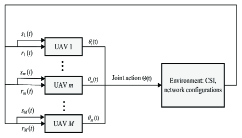
Figure 2: Illustration of MARL framework for multi-UAV networks.

Fig. 2 describes the key components of MARL studied in this article. Specifically, for each UAV $m$, the left-hand side of the box is the locally observed information at time slot $t$–state $s_{m}^{t}$ and reward $r_{m}^{t}$; the right-hand side of the box is the action for UAV $m$ at time slot $t$. The decision problem faced by a player in a stochastic game when all other players choose a fixed strategy profile is equivalent to an Markov decision processes (MDP) [26]. An agent-independent method is proposed, for which all agents conduct a decision algorithm independently but share a common structure based on Q-learning.

Since Markov property is used to model the dynamics of the environment, the rewards of UAVs are based only on the current state and action. MDP for agent (UAV) $m$ consists of: 1) a discrete set of environment state $\mathcal{S}_{m}$, 2) a discrete set of possible actions $\Theta_{m}$, 3) a one-slot dynamics of the environment given by the state transition probabilities $F_{s_{m}^{t}\rightarrow s_{m}^{t+1}}=F(s_{m}^{t},\theta,s_{m}^{t+1})$ for all $\theta_{m}\in\Theta_{m}$ and $s_{m}^{t},s_{m}^{t+1}\in\mathcal{S}_{m}$; 4) a reward function $R_{m}$ denoting the expected value of the next reward for UAV $m$. For instance, given the current state $s_{m}$, action $\theta_{m}$ and the next state $s_{m}^{\prime}$: $R_{m}(s_{m},\theta_{m},s_{m}^{\prime})=E\{r_{m}^{t+1}|s_{m}^{t}=s_{m},\theta_{m}^{t}=\theta_{m},s_{m}^{t+1}=s_{m}^{\prime}\}$, where $r_{m}^{t+1}$ denotes the immediate reward of the environment to UAV $m$ at time $t+1$. Notice that UAVs cannot interact with each other, hence each UAV knows imperfect information of its operating stochastic environment. In this article, Q-learning is used to solve MDPs, for which a learning agent operates in an unknown stochastic environment and does not know the reward and transition functions [33]. Next we describe the Q-learning algorithm for solving the MDP for one UAV. Without loss of generalities, UAV $m$ is considered for simplicity. Two fundamental concepts of algorithms for solving the above MDP is the state value function and action value function (Q-function) [34]. Specifically, the former in fact is the expected reward for some state in (22) giving the agent in following some policy. Similarly, the Q-function for UAV $m$ is the expected reward starting from the state $s_{m}$, taking the action $\theta_{m}$ and following policy $\pi$, which can be expressed as

$$\begin{aligned} Q_{m}(s_{m},\theta_{m},\pi)=E\bigg{\{}\sum_{\tau=0}^{+\infty}\delta^{\tau}r_{m}^{t+\tau+1}\mid s^{t}=s,\theta_{m}^{t}=\theta_{m}\bigg{\}},\end{aligned}$$ (24)

where the corresponding values of (24) are called action values (Q-values).

Proposition 1.

A recursive relationship for the state value function can be derived from the established return. Specifically, for any strategy $\pi$ and any state $s_{m}$, the following condition holds between two consistency states $s_{m}^{t}=s_{m}$ and $s_{m}^{t+1}=s^{\prime}_{m}$, with $s_{m},~{}s^{\prime}_{m}\in\mathcal{S}_{m}$:

$$\begin{aligned} V_{m}(s_{m},\pi)&=E\left\{\sum_{\tau=0}^{+\infty}\delta^{\tau}r_{m}^{t+\tau+1}|s_{m}^{t}=s_{m}\right\}\\ &=\sum_{s^{\prime}_{m}\in\mathcal{S}_{m}}F(s_{m},\theta,s^{\prime}_{m})\sum_{\theta\in\Theta}\prod_{j\in\mathcal{M}}\pi_{j}(s_{j},\theta_{j})\times\left[R_{m}(s_{m},\theta,s^{\prime}_{m})+\delta V(s^{\prime}_{m},\pi)\right],\end{aligned}$$ (25)

where $\pi_{j}(s_{j},\theta_{j})$ is the probability of choosing action $\theta_{j}$ in state $s_{j}$ for UAV $m$.

Proof.

See Appendix A. ∎

Note that the state value function $V_{m}(s_{m},\pi)$ is the expected return when starting in state $s_{m}$ and following a strategy $\pi$ thereafter. Based on Proposition 1, we can rewrite the Q-function in (24) also into a recursive from, which is given by

$$\begin{aligned} &Q_{m}(s_{m},\theta_{m},\pi)=E\bigg{\{}r_{m}^{t+1}+\delta\sum_{\tau=0}^{+\infty}\delta^{\tau}r_{m}^{t+\tau+2}|s_{m}^{t}=s_{m},\theta_{m}^{t}=\theta,s_{m}^{t+1}=s^{\prime}_{m}\bigg{\}}\\ &\quad=\sum_{s^{\prime}_{m}\in\mathcal{S}_{m}}F(s_{m},\theta,s^{\prime}_{m})\sum_{\theta_{-m}\in\Theta_{-m}}\prod_{j\in\mathcal{M}\setminus\{m\}}\pi_{j}(s_{j},\theta_{j})\times\left[R(s_{m},\theta,s^{\prime}_{m})+\delta V_{m}(s^{\prime}_{m},\pi)\right].\end{aligned}$$ (26)

Note that from (26), Q-values depend on the actions of all the UAVs. It should be pointed out that (25) and (26) are the basic equations for the Q-learning based reinforcement learning algorithm for solving the MDP of each UAV. From (25) and (26), we also can derive the following relationship between state values and Q-values:

$$\begin{aligned} V_{m}(s_{m},\pi)=\sum_{\theta_{m}\in\Theta_{m}}\pi_{m}(s_{m},\theta_{m})Q_{m}(s_{m},\theta_{m},\pi).\end{aligned}$$ (27)

As discussed above, the goal of solving a MDP is to find an optimal strategy to obtain a maximal reward. An optimal strategy for UAV $m$ at state $s_{m}$, can be defined, from the perspective of state value function, as

$$\begin{aligned} V_{m}^{*}=\max_{\pi_{m}}V_{m}(s_{m},\pi),~{}~{}s_{m}\in\mathcal{S}_{m}.\end{aligned}$$ (28)

For the optimal Q-values, we also have

$$\begin{aligned} Q_{m}^{*}(s_{m},\theta_{m})=\max_{\pi_{m}}Q_{m}(s_{m},\theta_{m},\pi),s_{m}\in\mathcal{S}_{m},\theta_{m}\in\Theta_{m}.\end{aligned}$$ (29)

Substituting (27) to (28), the optimal state value equation in (28) can be reformulated as

$$\begin{aligned} V_{m}^{*}(s_{m})=\max_{\theta_{m}}Q_{m}^{*}(s_{m},\theta_{m}),\end{aligned}$$ (30)

where the fact that $\sum_{\theta_{m}}\pi(s_{m},\theta_{m})Q_{m}^{*}(s_{m},\theta_{m})\leq\max_{\theta_{m}}Q_{m}^{*}(s_{m},\theta_{m})$ was applied to obtain (30). Note that in (30), the optimal state value equation is a maximization over the action space instead of the strategy space.

Next by combining (30) with (25) and (26), one can obtain the Bellman optimality equations, for state values and for Q-values, respectively:

$$\begin{aligned} &V_{m}^{*}(s_{m})=\sum_{\theta_{-m}\in\Theta_{-m}}\prod_{j\in\mathcal{M}\setminus\{m\}}\pi_{j}(s_{j},\theta_{j})\times\max_{\theta_{m}}\sum_{s^{\prime}_{m}}F(s_{m},\theta,s^{\prime}_{m})\left[R(s_{m},\theta_{m},s^{\prime}_{m})+\delta V_{m}^{*}(s^{\prime}_{m})\right],\end{aligned}$$ (31)

and

$$\begin{aligned} &Q_{m}^{*}(s_{m},\theta_{m})=\\ &\sum_{\theta_{-m}\in\Theta_{-m}}\prod_{j\in\mathcal{M}\setminus\{m\}}\pi_{j}(s_{j},\theta_{j})\times\sum_{s^{\prime}_{m}}F(s_{m},\theta,s^{\prime}_{m})\bigg{[}R(s_{m},\theta_{m},s^{\prime}_{m})+\delta\max_{\theta^{\prime}_{m}}Q_{m}^{*}(s^{\prime}_{m},\theta^{\prime}_{m})\bigg{]}.\end{aligned}$$ (32)

Note that (32) indicates that the optimal strategy will always choose an action that maximizes the Q-function for the current state. In the multi-agent case, the Q-function of each agent depends on the joint action and is conditioned on the joint policy, which makes it complex to find an optimal joint strategy [34]. To overcome these challenges, we consider UAV are independent learners (ILs), that is UAVs do not observe the rewards and actions of the other UAVs, they interact with the environment as if no other UAUs exist.

IV-B Q-Learning based Resource Allocation for Multi-UAV Networks

In this subsection, an ILs [35] based MARL algorithm is proposed to solve the resource allocation among UAVs. Specifically, each UAV runs a standard Q-learning algorithm to learn its optimal Q-values and simultaneously determines an optimal strategy for the MDP. Specifically, the selection of an action in each iteration depends on Q-values in terms of two states- $s_{m}$ and its successors. Hence Q-values provide insights on the future quality of the actions in the successor state. The update rule for Q-learning [33] is given by

$$\begin{aligned} &Q_{m}^{t+1}(s_{m},\theta_{m})=Q_{m}^{t}(s_{m},\theta_{m})+\alpha^{t}\bigg{\{}r_{m}^{t}+\delta\max_{\theta^{\prime}_{m}\in\Theta_{m}}Q_{m}^{t}(s^{\prime}_{m},\theta^{\prime}_{m})-Q_{m}^{t}(s_{m},\theta_{m})\bigg{\}},\end{aligned}$$ (33)

with $s_{m}^{t}=s_{m},~{}\theta_{m}^{t}=\theta_{m}$, where $s^{\prime}_{m}$ and $\theta^{\prime}_{m}$ correspond to $s_{m}^{t+1}$ and $\theta_{m}^{t+1}$, respectively. Note that an optimal action-value function can be obtained recursively from the corresponding action-values. Specifically, each agent learns the optimal action-values based on the updating rule in (33), where $\alpha_{t}$ denotes the learning rate and $Q_{m}^{t}$ is the action-value of UAV $m$ at time slot $t$.

Another important component of Q-learning is action selection mechanisms, which are used to select the actions that the agent will perform during the learning process. Its purpose is to strike a balance between exploration and exploitation that the agent can reinforce the evaluation it already knows to be good but also explore new actions [33]. In this article, we consider $\epsilon$-greedy exploration. In $\epsilon$-greedy selection, the agent selects a random action with probability $\epsilon$ and selects the best action, which corresponds to the highest Q-value at the moment, with probability $1-\epsilon$. As such, the probability of selecting action $\theta_{m}$ at state $s_{m}$ is given by

$$\begin{aligned} \pi_{m}(s_{m},\theta_{m})=\begin{cases}1-\epsilon,~{}\text{if}~{}Q_{m}~{}\text{of}~{}\theta_{m}\text{is the highest},\\ \epsilon,~{}\text{otherwise}.\end{cases}\end{aligned}$$ (34)

where $\epsilon\in(0,1)$. To ensure the convergence of Q-learning, the learning rate $\alpha_{t}$ are set as in [36], which is given by

$$\begin{aligned} \alpha_{t}=\frac{1}{(t+c_{\alpha})^{\varphi_{\alpha}}},\end{aligned}$$ (35)

where $c_{\alpha}>0$, $\varphi_{\alpha}\in(\frac{1}{2},1]$ .

Note that each UAV runs the Q-learning procedure independently in the proposed ILs based MARL algorithm. Hence, for each UAV $m$, $m\in\mathcal{M}$, the Q-learning procedure is concluded in Algorithm 1. In Algorithm 1, the initial Q-values are set to zero, therefore, it is also called zero-initialized Q-learning [37]. Since UAVs have no prior information on the initial state, a UAV takes a strategy with equal probabilities, i.e., $\pi_{m}(s_{m},\theta_{m})=\frac{1}{|\Theta_{m}|}$.

Algorithm 1 Q-learning based MARL algorithm for UAVs

1:  Initialization:

2:  Set $t=0$ and the parameters $\delta,~{}c_{\alpha}$

3:  for all  $m\in\mathcal{M}$ do

4:     Initialize the action-value $Q_{m}^{t}(s_{m},\theta_{m})=0$, strategy $\pi_{m}(s_{m},\theta_{m})=\frac{1}{|\Theta_{m}|}=\frac{1}{MKJ}$;

5:     Initialize the state $s_{m}=s_{m}^{t}=0$;

6:  end for

7:  Main Loop:

8:  while $t<T$ do

9:     for all UAV $m$, $m\in\mathcal{M}$ do

10:        Update the learning rate $\alpha_{t}$ according to (35).

11:        Select an action $\theta_{m}$ according to the strategy $\pi_{m}(s_{m})$.

12:        Measure the achieved SINR at the receiver according to (16);

13:        if $\gamma_{m}(t)\geq\bar{\gamma}_{m}$ then

14:           Set $s_{m}^{t}=1$.

15:        else

16:           Set $s_{m}^{t}=0$.

17:        end if

18:        Update the instantaneous reward $r_{m}^{t}$ according to (20).

19:        Update the action-value $Q_{m}^{t+1}(s_{m},\theta_{m})$ according to (33).

20:        Update the strategy $\pi_{m}(s_{m},\theta_{m})$ according to (34).

21:        Update $t=t+1$ and the state $s_{m}=s_{m}^{t}$.

22:     end for

23:  end while

IV-C Analysis of the proposed MARL algorithm

In this subsection, we investigate the convergence of the proposed MARL based resource allocation algorithm. Notice that the proposed MARL algorithm can be treated as an independent multi-agent Q-learning algorithm, in which each UAV as a learning agent makes a decision based on the Q-learning algorithm. Therefore, the convergence is concluded in the following proposition.

Proposition 2.

In the proposed MARL algorithm of Algorithm 1, the Q-learning procedure for each UAV is always converged to the Q-value for individual optimal strategy.

The proof of Proposition 2 depends on the following observations. Due to the non-cooperative property of UAVs, the convergence of the proposed MARL algorithm is dependent on the convergence of Q-learning algorithm [35]. Therefore, we focus on the proof of convergence for the Q-learning algorithm in Algorithm 1.

Theorem 1.

The Q-learning algorithm in Algorithm 1 with the update rule in (33) converges with probability one (w.p.1) to the optimal $Q_{m}^{*}(s_{m},\theta_{m})$ value if

1. The state and action spaces are finite;

2. $\sum_{t=0}^{+\infty}\alpha^{t}=\infty$, $\sum_{t=0}^{+\infty}(\alpha^{t})^{2}<\infty$ uniformly w.p. 1;

3. $\mathrm{Var}\{r_{m}^{t}\}$ is bounded;

Proof.

See Appendix B.

∎

V Simulation Results

In this section, we verify the effectiveness of the proposed MARL based resource allocation algorithm for multi-UAV networks by simulations. We consider multi-UAV networks deployed in a disc area with a radius $r_{d}=500$ m. The ground users are randomly and uniformly distributed inside the disk. All UAVs are assumed to fly at a fixed altitude $H=100$ m. In the simulations, the noise power is assumed to be $\sigma^{2}=-80$ dBm, the subchannel bandwidth is $\frac{W}{K}=75$ KHz and $Ts=0.1$ s. For the probabilistic model, the channel parameters in the simulations follow [7], where $\mathfrak{a}=9.61$ and $\mathfrak{b}=0.16$. Moreover, the carrier frequency is $f=2$ GHz, $\eta^{\mathrm{LoS}}=1$ and $\eta^{\mathrm{NLoS}}=20$. For the LoS channel model, the channel power gain at reference distance $d_{0}=1$ m is set as $\beta_{0}=-60$ dB and the path loss coefficient is set as $\alpha=2$ [11]. In the simulations, the maximal power level number is $J=3$, the maximal power for each UAV is $P_{m}=P=23$ dBm, where the maximal power is equally divided into $J$ discrete power values. The cost per unit level of power is $\omega_{m}=\omega=100$ and the minimum SINR for the users is set as $\gamma_{0}=3$ dB. Moreover, $c_{\alpha}=0.5$, $\rho_{\alpha}=0.8$ and $\delta=1$.

In Fig. 3, we consider a random realization of a multi-UAV network in horizontal plane, where $L=100$ users are uniformly distributed in a disk with radius $r=500$ m and two UAVs are initially located at the edge of the disk with the angle $\phi=\frac{\pi}{4}$. For illustrative purposes, Fig. 4 shows the average reward and the average reward per time slot of the UAVs under the setup of Fig. 3, where the speed of the UAVs are set as $40$ m/s. Fig. 4(a) shows average rewards with different $\epsilon$, which is calculated as $v^{t}=\frac{1}{M}\sum_{m\in\mathcal{M}}v_{m}^{t}$. As can be observed from Fig. 4(a), the average reward increases with the algorithm iterations. This is because the long-term reward can be improved by the proposed MARL algorithm. However, the curves of the average reward become flat when $t$ is higher that 250 time slots. In fact, the UAVs will fly outside the disk when $t>250$. As a result, the average reward will not increase. Correspondingly, Fig. 4(b) illustrates the average instantaneous reward per time slot $r^{t}=\sum_{m\in\mathcal{M}}r_{m}^{t}$. As can be observed from Fig. 4(b), the average reward per time slot decreases with algorithm iterations. This is because that the learning rate $\alpha_{t}$ in the adopted Q-learning procedure is a function of $t$ in (35), where $\alpha_{t}$ decreases with time slots increasing. Notice that from (35), $\alpha_{t}$ will decrease with algorithm iterations, which means that the update rate of the Q-values becomes slow with increasing $t$. Moreover, Fig. 4 also investigates the average reward with different $\epsilon=\{0,~{}0.2,~{}0.5,~{}0.9\}$. If $\epsilon=0$, each UAV will choose a greedy action which is also called exploit strategy. If $\epsilon$ goes to 1, each UAV will choose a random action with higher probabilities. Notice that from Fig. 4, $\epsilon=0.5$ is a good choice in the considered setup.

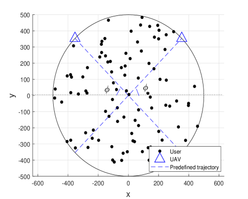
Figure 3: Illustration of UAVs based networks with $M=2$ and $L=100$.

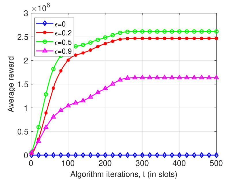
(a) Comparisons of average rewards.

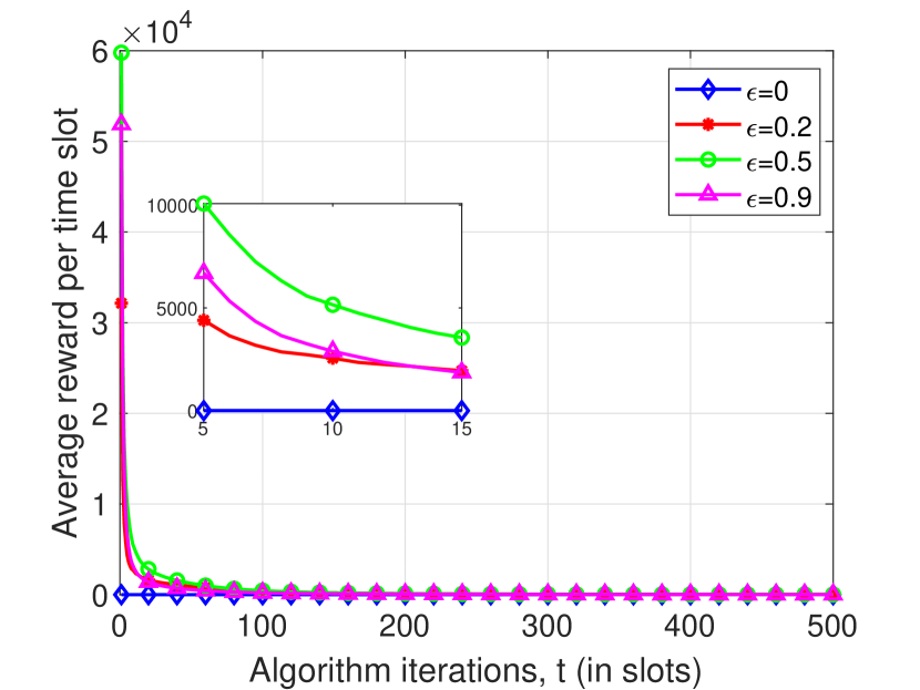
(b) Average rewards per time slot.

Figure 4: Comparisons for average rewards with different $\epsilon$, where $M=2$ and $L=100$.

In Fig. 5 and Fig. 6, we investigate the average reward under different system configurations. Fig. 5 illustrates the average reward with LoS channel model given in (4) over different $\epsilon$. Moreover, Fig. 6 illustrates the average reward under probabilistic model with $M=4,~{}K=3$ and $L=200$. Specifically, the UAVs randomly distributed in the cell edge. In the iteration procedure, each UAV flies over the cell followed by a straight line over the cell center, that is the center of the disk. As can be observed from Fig. 5 and Fig. 6, the curves of the average reward have the similar trends with that of Fig. 4 under different $\epsilon$. Besides, the considered multi-UAV network attains the optimal average reward when $\epsilon=0.5$ under different network configurations.

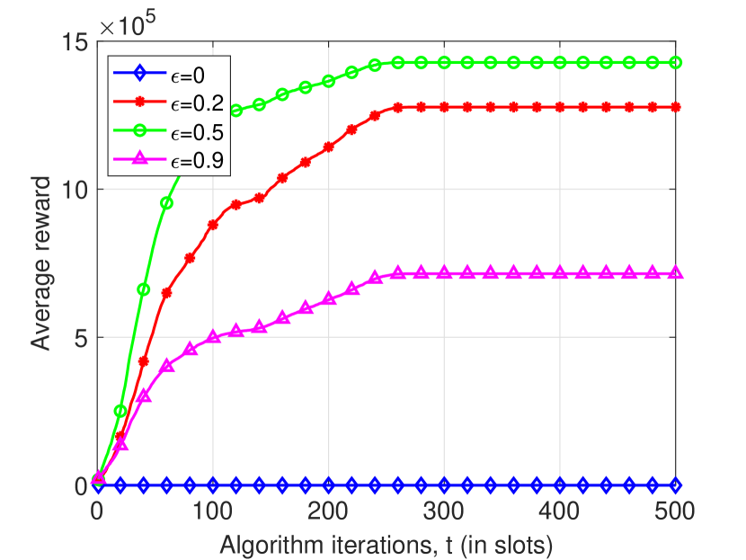
(a) Comparisons of average rewards.

(b) Average rewards per time slot.

Figure 5: LoS channel model with different $\epsilon$, where $M=2$ and $L=100$.

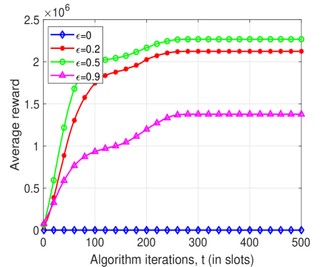
Figure 6: Illustration of multi-UAV networks with $M=4,~{}K=3$ and $L=200$.

In Fig. 7, we investigate the average reward of the proposed MARL algorithm by comparing it to the matching theory based resource allocation algorithm (Match). In Fig. 7, we consider the same setup as in Fig. 4 but with $J=1$ for the simiplicity of algorithm implementation, which indicates that the UAV’s action only contains the user selection for each time slot. Furthermore, we consider complete information exchanges among UAVs are performed in the matching theory based user selection algorithm, that is each UAV knows other UAVs’ action before making its own decision. comparisons, in the matching theory based user selection procedure, we adopt the Gale-Shapley (GS) algorithm [38] at each time slot. Moreover, we also consider the performance of the randomly user selection algorithm (Rand) as a baseline scheme in Fig. 7. As can be observed that from 7, the achieved average reward of the matching based user selection algorithm outperforms that of the proposed MARL algorithm. This is because there is not information exchanges in the proposed MARL algorithm. In this case, each UAV cannot observe the other UAVs’ information such as rewards and decisions, and thus it makes its decision independently. Moreover, it can be observed from Fig. 7, the average reward for the randomly user selection algorithm is lower than that of the proposed MARL algorithm. This is because of the randomness of user selections, it cannot exploit the observed information effectively. As a result, the proposed MARL algorithm can achieve a tradeoff between reducing the information exchange overhead and improving the system performance.

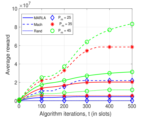
Figure 7: Comparisons of average rewards among different algorithms, where $M=2$, $K=1$, $J=1$ and $L=100$.

In Fig. 8, we investigate the average reward as a function of algorithm iterations and the UAV’s speed, where a UAU from a random initial location in the disc edge, flies over the disc along a direct line across the disc center with different speeds. The setup in Fig. 8 is the same as that in Fig. 6 but with $M=1$ and $K=1$ for illustrative purposes. As can be observed that for a fixed speed, the average reward increases monotonically with increasing the algorithm iterations. Besides, for a fixed time slot, the average reward of larger speeds increases faster than that with smaller speeds when $t$ is smaller than 150. This is due to the randomness of the locations for users and the UAV, at the start point the UAV may not find an appropriate user satisfying its QoS requirement. Fig. 8 also shows that the achieved average reward decreases when the speed increases at the end of algorithm iterations. This is because that if the UAV flies with a high speed, it will take less time to fly out the disc. As a result, the UAV with higher speeds has less serving time than that of slower speeds.

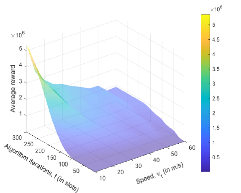
Figure 8: Average rewards with different time slots and speeds.

VI Conclusions

In this article, we investigated the real-time designs of resource allocation for multi-UAV downlink networks to maximize the long-term rewards. Motivated by the uncertainty of environments, we proposed a stochastic game formulation for the dynamic resource allocation problem of the considered multi-UAV networks, in which the goal of each UAV was to find a strategy of the resource allocation for maximizing its expected reward. To overcome the overhead of the information exchange and computation, we developed an ILs based MARL algorithm to solve the formulated stochastic game, where all UAVs conducted a decision independently based on Q-learning. Simulation results revealed that the proposed MARL based resource allocation algorithm for the multi-UAV networks can attain a tradeoff between the information exchange overhead and the system performance. One promising extension of this work is to consider more complicated joint learning algorithms for multi-UAV networks with the partial information exchanges, that is the need of cooperation. Moreover, incorporating the optimization of deployment and trajectories of UAVs into multi-UAV networks is capable of further improving energy efficiency of multi-UAV networks, which is another promising future research direction.

Appendix A: Proof of Proposition 1

Here, we show that the state values for one UAV $m$ over time in (25). For one UAV $m$ with state $s_{m}\in\mathcal{S}_{m}$ at time step $t$, its state value function can be expressed as

$$\begin{aligned} &V(s_{m},\pi)=E\left\{\sum_{\tau=0}^{+\infty}\delta^{\tau}r_{m}^{t+\tau+1}|s_{m}^{t}=s_{m}\right\}\\ &=E\left\{r_{m}^{t+1}+\delta\sum_{\tau=0}^{+\infty}\delta^{\tau}r_{m}^{t+\tau+2}|s_{m}^{t}=s_{m}\right\}\\ &=E\left\{r_{m}^{t+1}|s_{m}^{t}=s_{m}\right\}+\delta E\left\{\sum_{\tau=0}^{+\infty}\delta^{\tau}r_{m}^{t+\tau+2}|s_{m}^{t}=s_{m}\right\},\end{aligned}$$ (A.1)

where the first part and the second part represent the expected value and the state value function, respectively, at time $t+1$ over the state space and the action space. Next we show the relationship between the first part and the reward function $R(s_{m},\theta,s_{m}^{\prime})$ with $s_{m}^{t}=s_{m},~{}\theta_{m}^{t}=\theta$ and $s_{m}^{t+1}=s^{\prime}_{m}$.

$$\begin{aligned} &E\left\{r_{m}^{t+1}|s_{m}^{t}=s_{m}\right\}\\ &=\sum_{s^{\prime}_{m}\in\mathcal{S}_{m}}F(s_{m},\theta,s^{\prime}_{m})\sum_{\theta\in\Theta}\prod_{j\in\mathcal{M}}\pi_{j}(s_{j},\theta_{j})\times E\left\{r^{t+1}|s_{m}^{t}=s_{m},\theta_{m}^{t}=\theta_{m},s_{m}^{t+1}=s^{\prime}_{m}\right\}\\ &=\sum_{s^{\prime}_{m}\in\mathcal{S}_{m}}F(s_{m},\theta,s^{\prime}_{m})\sum_{\theta\in\Theta}\prod_{j\in\mathcal{M}}\pi_{j}(s_{j},\theta_{j})R_{m}(s_{m},\theta,s^{\prime}_{m}),\end{aligned}$$ (A.2)

where the definition of $R_{m}(s_{m},\theta,s^{\prime}_{m})$ has been used to obtain the final step. Similarly, the second part can be transformed into

$$\begin{aligned} &E\left\{\sum_{\tau=0}^{+\infty}\delta^{\tau}r_{m}^{t+\tau+2}|s_{m}^{t}=s_{m}\right\}\\ &=\sum_{s^{\prime}_{m}\in\mathcal{S}_{m}}F(s_{m},\theta,s^{\prime}_{m})\sum_{\theta\in\Theta}\prod_{j\in\mathcal{M}}\pi_{j}(s_{j},\theta_{j})\times E\left\{\sum_{\tau=0}^{+\infty}\delta^{\tau}r_{m}^{t+\tau+2}|s_{m}^{t}=s_{m},\theta_{m}^{t}=\theta_{m},s_{m}^{t+1}=s^{\prime}_{m}\right\}\\ &=\sum_{s^{\prime}_{m}\in\mathcal{S}_{m}}F(s_{m},\theta,s^{\prime}_{m})\sum_{\theta\in\Theta}\prod_{j\in\mathcal{M}}\pi_{j}(s_{j},\theta_{j})V(s^{\prime}_{m},\pi).\end{aligned}$$ (A.3)

Substituting (A.2) and (A.3) into (A.1), we get

$$\begin{aligned} &V(s_{m},\pi)=\sum_{s^{\prime}_{m}\in\mathcal{S}_{m}}F(s_{m},\theta,s^{\prime}_{m})\sum_{\theta\in\Theta}\prod_{j\in\mathcal{M}}\pi_{j}(s_{j},\theta_{j})\times\left[R_{m}(s_{m},\theta,s^{\prime}_{m})+\delta V(s^{\prime}_{m},\pi)\right].\end{aligned}$$ (A.4)

Thus, Proposition 1 is proved.

Appendix B: Proof of Theorem 1

The proof of Theorem 1 follows from the idea in [36, 39]. Here we give a more general procedure for Algorithm 1. Note that the Q-learning algorithm is a stochastic form of value iteration [36], which can be observed from (26) and (32). That is to perform a step of value iteration requires knowing the expected reward and the transition probabilities. Therefore, to prove the convergence of the Q-learning algorithm, stochastic approximation theory is applied. We first introduce a result of stochastic approcximation given in [36].

Lemma 1.

A random iterative process $\bigtriangleup^{t+1}(x)$, which is defined as

$$\bigtriangleup^{t+1}(x)=(1-\alpha^{t}(x))\bigtriangleup^{t}(x)+\beta^{t}(x)\Psi^{t}(x),$$ (B.1)

converges to zero w.p.1 if and only if the following conditions are satisfied.

1. The state space is finite;

2. $\sum_{t=0}^{+\infty}\alpha^{t}=\infty$, $\sum_{t=0}^{+\infty}(\alpha^{t})^{2}<\infty$, $\sum_{t=0}^{+\infty}\beta^{t}=\infty$, $\sum_{t=0}^{+\infty}(\beta^{t})^{2}<\infty$, and $E\{\beta^{t}(x)|\Lambda^{t}\}\leq E\{\alpha^{t}(x)|\Lambda^{t}\}$ uniformly w.p. 1;

3. $\|E\{\Psi^{t}(x)|\Lambda^{t}\}\|_{W}\leq\varrho\|\bigtriangleup^{t}\|_{W}$, where $\varrho\in(0,1)$;

4. $\mathrm{Var}\{\Psi^{t}(x)|\Lambda^{t}\}\leq C(1+\|\bigtriangleup^{t}\|_{W})^{2}$, where $C>0$ is a constant.

Note that $\Lambda^{t}=\{\bigtriangleup^{t},\bigtriangleup^{t-1},\cdots,\Psi^{t-1},\cdots,\alpha^{t-1},\cdots,\beta^{t-1}\}$ denotes the past at time slot $t$. $\|\cdot\|_{W}$ denotes some weighted maximum norm.

Based on the results given in Lemma 1, we now prove Theorem 1 as follows.

Note that the Q-learning update equation in (33) can be rearranged as

$$\begin{aligned} Q_{m}^{t+1}(s_{m},\theta_{m})=&(1-\alpha^{t})Q_{m}^{t}(s_{m},\theta_{m})+\alpha^{t}\big{\{}r_{m}^{t}+\delta\max_{\theta^{\prime}_{m}\in\Theta_{m}}Q_{m}^{t}(s^{\prime}_{m},\theta^{\prime}_{m})\big{\}}.\end{aligned}$$ (B.2)

By subtracting $Q_{m}^{*}(s_{m},\theta_{m})$ from both side of (B.2), we have

$$\begin{aligned} &\bigtriangleup_{m}^{t+1}(s_{m},\theta_{m})=(1-\alpha^{t})\bigtriangleup_{m}^{t}(s_{m},\theta_{m})+\alpha^{t}\delta\Psi^{t}(s_{m},\theta_{m}),\end{aligned}$$ (B.3)

where

$$\bigtriangleup_{m}^{t}(s_{m},\theta_{m})=Q_{m}^{t}(s_{m},\theta_{m})-Q_{m}^{*}(s_{m},\theta_{m}),$$ (B.4)

$$\Psi_{m}^{t}(s_{m},\theta_{m})=r_{m}^{t}+\delta\max_{\theta^{\prime}_{m}\in\Theta_{m}}Q_{m}^{t}(s^{\prime}_{m},\theta^{\prime}_{m})-Q_{m}^{*}(s_{m},\theta_{m}).$$ (B.5)

Therefore, the Q-learning algorithm can be seen as the random process of Lemma 1 with $\beta^{t}=\alpha^{t}$.

Next we prove that the $\Psi^{t}(s_{m},\theta_{m})$ has the properties of 3) and 4) in Lemma 1. We start by showing that $\Psi^{t}(s_{m},\theta_{m})$ is a contraction mapping with respect to some maximum norm.

Definition 4.

For a set $\mathcal{X}$, a mapping $\mathbf{H}:~{}\mathcal{X}\rightarrow\mathcal{X}$ is a contraction mapping, or contraction, if there exists a constant $\delta$, with $delta\in(0,1)$, such that

$$\begin{aligned} \|\mathbf{H}x_{1}-\mathbf{H}x_{2}\|\leq\delta\|x_{1}-x_{2}\|,\end{aligned}$$ (B.6)

for any $x_{1},x_{2}\in\mathcal{X}$.

Proposition 3.

There exists a contraction mapping $\mathbf{H}$ for the function $q$ with the form of the optimal Q-function in (B.8). That is

$$\begin{aligned} &\|\mathbf{H}q_{1}(s_{m},\theta_{m})-\mathbf{H}q_{2}(s_{m},\theta_{m})\|_{\infty}\leq\delta\|q_{1}(s_{m},\theta_{m})-q_{2}(s_{m},\theta_{m})\|_{\infty},\end{aligned}$$ (B.7)

Proof.

From (32), the optimal Q-function for Algorithm 1 can be expressed as

$$\begin{aligned} Q_{m}^{*}(s_{m},\theta_{m})&=\sum_{s^{\prime}_{m}}F(s_{m},\theta_{m},s^{\prime}_{m})\times\big{[}R(s_{m},\theta_{m},s^{\prime}_{m})+\delta\max_{\theta^{\prime}_{m}}Q_{m}^{*}(s^{\prime}_{m},\theta^{\prime}_{m})\big{]}.\end{aligned}$$ (B.8)

Hence, we have

$$\begin{aligned} \mathbf{H}q(s_{m},\theta_{m})&=\sum_{s^{\prime}_{m}}F(s_{m},\theta_{m},s^{\prime}_{m})\times\big{[}R(s_{m},\theta_{m},s^{\prime}_{m})+\delta\max_{\theta^{\prime}_{m}}q(s^{\prime}_{m},\theta^{\prime}_{m})\big{]}.\end{aligned}$$ (B.9)

To obtain (B.7), we make the following calculations in (B.10). Note that the definition of $q$ is used in (a), (b) and (c) follows properties of absolute value inequalities. Moreover, (d) comes from the definition of infinity norm and (e) is based on the maximum calculation.

$$\begin{aligned} &\|\mathbf{H}q_{1}(s_{m},\theta_{m})-\mathbf{H}q_{2}(s_{m},\theta_{m})\|_{\infty}\stackrel{{\scriptstyle\mathrm{(a)}}}{{=}}\max_{s_{m},\theta_{m}}\delta\bigg{|}\sum_{s^{\prime}_{m}}F(s_{m},\theta_{m},s^{\prime}_{m})\big{[}\max_{\theta^{\prime}_{m}}q_{1}(s^{\prime}_{m},\theta^{\prime}_{m})-\max_{\theta^{\prime}_{m}}q_{2}(s^{\prime}_{m},\theta^{\prime}_{m})\big{]}\bigg{|}\\ &\stackrel{{\scriptstyle\mathrm{(b)}}}{{\leq}}\max_{s_{m},\theta_{m}}\delta\sum_{s^{\prime}_{m}}F(s_{m},\theta_{m},s^{\prime}_{m})\bigg{|}\max_{\theta^{\prime}_{m}}q_{1}(s^{\prime}_{m},\theta^{\prime}_{m})-\max_{\theta^{\prime}_{m}}q_{2}(s^{\prime}_{m},\theta^{\prime}_{m})\bigg{|}\\ &\stackrel{{\scriptstyle\mathrm{(c)}}}{{\leq}}\max_{s_{m},\theta_{m}}\delta\sum_{s^{\prime}_{m}}F(s_{m},\theta,s^{\prime}_{m})\max_{\theta^{\prime}_{m}}\bigg{|}q_{1}(s^{\prime}_{m},\theta^{\prime}_{m})-q_{2}(s^{\prime}_{m},\theta^{\prime}_{m})\bigg{|}\\ &\stackrel{{\scriptstyle\mathrm{(d)}}}{{=}}\max_{s_{m},\theta_{m}}\delta\sum_{s^{\prime}_{m}}F(s_{m},\theta,s^{\prime}_{m})\|q_{1}(s^{\prime}_{m},\theta^{\prime}_{m})-q_{2}(s^{\prime}_{m},\theta^{\prime}_{m})\|_{\infty}\stackrel{{\scriptstyle\mathrm{(e)}}}{{=}}\delta\|q_{1}(s^{\prime}_{m},\theta^{\prime}_{m})-q_{2}(s^{\prime}_{m},\theta^{\prime}_{m})\|_{\infty}\end{aligned}$$ (B.10)

∎

Based on (B.5) and (B.9),

$$\begin{aligned} E\{\Psi^{t}(s_{m},\theta_{m})\}&=\sum_{s^{\prime}_{m}}F(s_{m},\theta,s^{\prime}_{m})\times\big{[}r_{m}^{t}+\delta\max_{\theta^{\prime}_{m}\in\Theta_{m}}Q_{m}^{t}(s^{\prime}_{m},\theta^{\prime}_{m})-Q_{m}^{*}(s_{m},\theta_{m})\big{]}\\ &=\mathbf{H}Q^{t}_{m}(s_{m},\theta_{m})-Q_{m}^{*}(s_{m},\theta_{m})\\ &=\mathbf{H}Q^{t}_{m}(s_{m},\theta_{m})-\mathbf{H}Q_{m}^{*}(s_{m},\theta_{m}).\end{aligned}$$ (B.11)

where we have used the fact that $Q_{m}^{*}(s_{m},\theta_{m})=\mathbf{H}Q^{*}_{m}(s_{m},\theta_{m})$ since $Q_{m}^{*}(s_{m},\theta_{m})$ is a some constant value. As a result, we can obtain from Proposition 3 and (B.4) that

$$\begin{aligned} \|E\{\Psi^{t}(s_{m},\theta_{m})\}\|_{\infty}&\leq\delta\|Q^{t}_{m}(s_{m},\theta_{m})-Q_{m}^{*}(s_{m},\theta_{m})\|_{\infty}\\ &=\delta\|\bigtriangleup_{m}^{t}(s_{m},\theta_{m})\|_{\infty},\end{aligned}$$ (B.12)

Note that (B.12) corresponds to condition 3) of Lemma 1 in the form of infinity norm.

Finally, we verify the condition in 4) of Lemma 1 is satisfied.

$$\begin{aligned} &\mathrm{Var}\{\Psi^{t}(s_{m},\theta_{m})\}\\ &=E\{r_{m}^{t}+\delta\max_{\theta^{\prime}_{m}\in\Theta_{m}}Q_{m}^{t}(s^{\prime}_{m},\theta^{\prime}_{m})-Q_{m}^{*}(s_{m},\theta_{m})-\mathbf{H}Q^{t}_{m}(s_{m},\theta_{m})+Q_{m}^{*}(s_{m},\theta_{m})\}\\ &=E\{r_{m}^{t}+\delta\max_{\theta^{\prime}_{m}\in\Theta_{m}}Q_{m}^{t}(s^{\prime}_{m},\theta^{\prime}_{m})-\mathbf{H}Q^{t}_{m}(s_{m},\theta_{m})\}\\ &=\mathrm{Var}\{r_{m}^{t}+\delta\max_{\theta^{\prime}_{m}\in\Theta_{m}}Q_{m}^{t}(s^{\prime}_{m},\theta^{\prime}_{m})\}\\ &\leq C(1+\|\bigtriangleup_{m}^{t}(s_{m},\theta_{m})\|_{W}^{2}),\end{aligned}$$ (B.13)

where $C$ is some constant. The final step is based on the fact that the variance of $r_{m}^{t}$ is bounded and $Q_{m}^{t}(s^{\prime}_{m},\theta^{\prime}_{m})$ at most linearly.

Therefore, $\|\bigtriangleup_{m}^{t}(s_{m},\theta_{m})\|$ converges to zero w.p.1 in Lemma 1, which indicates $Q_{m}^{t}(s_{m},\theta_{m})$ converges to $Q_{m}^{*}(s_{m},\theta_{m})$ w.p.1 in Theorem 1.

References

- [1] I. Bucaille, S. Héthuin, A. Munari, R. Hermenier, T. Rasheed, and S. Allsopp, “Rapidly deployable network for tactical applications: Aerial base station with opportunistic links for unattended and temporary events ABSOLUTE example,” in IEEE Proc. of Mil. Commun. Conf. (MILCOM), Nov. 2013, pp. 1116–1120.
- [2] S. Chandrasekharan, K. Gomez, A. Al-Hourani, S. Kandeepan, T. Rasheed, L. Goratti, L. Reynaud, D. Grace, I. Bucaille, T. Wirth, and S. Allsopp, “Designing and implementing future aerial communication networks,” IEEE Commun. Mag., vol. 54, no. 5, pp. 26–34, May 2016.
- [3] A. Al-Hourani, S. Kandeepan, and S. Lardner, “Optimal LAP altitude for maximum coverage,” IEEE Wireless Commun. Lett., vol. 3, no. 6, pp. 569–572, Dec. 2014.
- [4] M. Mozaffari, W. Saad, M. Bennis, Y. Nam, and M. Debbah, “A tutorial on UAVs for wireless networks: Applications, challenges, and open problems,” CoRR, vol. abs/1803.00680, 2018. [Online]. Available: http://arxiv.org/abs/1803.00680
- [5] M. Mozaffari, W. Saad, M. Bennis, and M. Debbah, “Drone small cells in the clouds: Design, deployment and performance analysis,” CoRR, vol. abs/1509.01655, 2015. [Online]. Available: http://arxiv.org/abs/1509.01655
- [6] ——, “Efficient deployment of multiple unmanned aerial vehicles for optimal wireless coverage,” IEEE Commun. Lett., vol. 20, no. 8, pp. 1647–1650, Aug. 2016.
- [7] M. Alzenad, A. El-Keyi, F. Lagum, and H. Yanikomeroglu, “3-D placement of an unmanned aerial vehicle base station (UAV-BS) for energy-efficient maximal coverage,” IEEE Wireless Commun. Lett., vol. 6, no. 4, pp. 434–437, Aug. 2017.
- [8] J. Lyu, Y. Zeng, R. Zhang, and T. J. Lim, “Placement optimization of UAV-mounted mobile base stations,” IEEE Commun. Lett., vol. 21, no. 3, pp. 604–607, Mar. 2017.
- [9] Y. Zeng, R. Zhang, and T. J. Lim, “Throughput maximization for UAV-enabled mobile relaying systems,” IEEE Trans. Commun., vol. 64, no. 12, pp. 4983–4996, Dec. 2016.
- [10] Y. Zeng, X. Xu, and R. Zhang, “Trajectory design for completion time minimization in UAV-enabled multicasting,” IEEE Trans. Wireless Commun., vol. 17, no. 4, pp. 2233–2246, Apr. 2018.
- [11] Q. Wu, Y. Zeng, and R. Zhang, “Joint trajectory and communication design for multi-UAV enabled wireless networks,” IEEE Trans. Wireless Commun., vol. 17, no. 3, pp. 2109–2121, Mar. 2018.
- [12] S. Zhang, H. Zhang, B. Di, and L. Song, “Cellular UAV-to-X communications: Design and optimization for multi-UAV networks in 5G,” 2018.
- [13] B. Geiger and J. Horn, “Neural network based trajectory optimization for unmanned aerial vehicles,” in 47th AIAA Aerospace Sciences Meeting Including the New Horizons Forum and Aerospace Exposition, 2009, p. 54.
- [14] D. Nodland, H. Zargarzadeh, and S. Jagannathan, “Neural network-based optimal control for trajectory tracking of a helicopter UAV,” in IEEE Conference on Decision and Control and European Control Conference, Dec. 2011, pp. 3876–3881.
- [15] Q. Zhang, M. Mozaffari, W. Saad, M. Bennis, and M. Debbah, “Machine learning for predictive on-demand deployment of UAVs for wireless communications,” arXiv preprint arXiv:1805.00061, 2018.
- [16] U. Challita, W. Saad, and C. Bettstetter, “Cellular-connected UAVs over 5G: Deep reinforcement learning for interference management,” CoRR, vol. abs/1801.05500, 2018. [Online]. Available: http://arxiv.org/abs/1801.05500
- [17] M. Chen, W. Saad, and C. Yin, “Liquid state machine learning for resource allocation in a network of cache-enabled LTE-U UAVs,” in IEEE Proc. of Global Commun. Conf. (GLOBECOM), Dec 2017, pp. 1–6.
- [18] J. Chen, Q. Wu, Y. Xu, Y. Zhang, and Y. Yang, “Distributed demand-aware channel-slot selection for multi-UAV networks: A game-theoretic learning approach,” IEEE Access, vol. 6, pp. 14 799–14 811, 2018.
- [19] N. Sun and J. Wu, “Minimum error transmissions with imperfect channel information in high mobility systems,” in IEEE Proc. of Mil. Commun. Conf. (MILCOM), Nov. 2013, pp. 922–927.
- [20] Y. Cai, F. R. Yu, J. Li, Y. Zhou, and L. Lamont, “Medium access control for unmanned aerial vehicle (UAV) ad-hoc networks with full-duplex radios and multipacket reception capability,” IEEE Trans. Veh. Technol., vol. 62, no. 1, pp. 390–394, Jan. 2013.
- [21] H. Li, “Multi-agent Q-learning of channel selection in multi-user cognitive radio systems: A two by two case,” in IEEE International Conference on Systems, Man and Cybernetics, Oct. 2009, pp. 1893–1898.
- [22] A. Galindo-Serrano and L. Giupponi, “Distributed Q-learning for aggregated interference control in cognitive radio networks,” IEEE Trans. Veh. Technol., vol. 59, no. 4, pp. 1823–1834, May 2010.
- [23] A. Asheralieva and Y. Miyanaga, “An autonomous learning-based algorithm for joint channel and power level selection by D2D pairs in heterogeneous cellular networks,” IEEE Trans. Commun., vol. 64, no. 9, pp. 3996–4012, Sep. 2016.
- [24] J. Cui, Z. Ding, P. Fan, and N. Al-Dhahir, “Unsupervised machine learning based user clustering in mmWave-NOMA systems,” IEEE Trans. Wireless Commun., to be published.
- [25] A. Nowé, P. Vrancx, and Y.-M. De Hauwere, “Game theory and multi-agent reinforcement learning,” in Reinforcement Learning. Springer, 2012, pp. 441–470.
- [26] A. Neyman, “From Markov chains to stochastic games,” in Stochastic Games and Applications. Springer, 2003, pp. 9–25.
- [27] J. How, Y. Kuwata, and E. King, “Flight demonstrations of cooperative control for UAV teams,” in AIAA 3rd” Unmanned Unlimited” Technical Conference, Workshop and Exhibit, 2004, p. 6490.
- [28] J. Zheng, Y. Cai, Y. Liu, Y. Xu, B. Duan, and X. . Shen, “Optimal power allocation and user scheduling in multicell networks: Base station cooperation using a game-theoretic approach,” IEEE Trans. Wireless Commun., vol. 13, no. 12, pp. 6928–6942, Dec. 2014.
- [29] B. Uragun, “Energy efficiency for unmanned aerial vehicles,” in International Conference on Machine Learning and Applications and Workshops, vol. 2, Dec. 2011, pp. 316–320.
- [30] Y. Shoham and K. Leyton-Brown, Multiagent systems: Algorithmic, game-theoretic, and logical foundations. Cambridge University Press, 2008.
- [31] A. Neyman and S. Sorin, Stochastic games and applications. Springer Science & Business Media, 2003, vol. 570.
- [32] M. J. Osborne and A. Rubinstein, A course in game theory. MIT press, 1994.
- [33] R. S. Sutton and A. G. Barto, Reinforcement learning: An introduction. MIT press Cambridge, 1998.
- [34] G. Neto, “From single-agent to multi-agent reinforcement learning: Foundational concepts and methods,” Learning theory course, 2005.
- [35] L. Matignon, G. J. Laurent, and N. Le Fort-Piat, “Independent reinforcement learners in cooperative markov games: a survey regarding coordination problems,” The Knowledge Engineering Review, vol. 27, no. 1, pp. 1–31, 2012.
- [36] T. Jaakkola, M. I. Jordan, and S. P. Singh, “Convergence of stochastic iterative dynamic programming algorithms,” in Advances in neural information processing systems, 1994, pp. 703–710.
- [37] S. Koenig and R. G. Simmons, “Complexity analysis of real-time reinforcement learning applied to finding shortest paths in deterministic domains,” CARNEGIE-MELLON UNIV PITTSBURGH PA SCHOOL OF COMPUTER SCIENCE, Tech. Rep., 1992.
- [38] D. Gale and L. S. Shapley, “College admissions and the stability of marriage,” The American Mathematical Monthly, vol. 69, no. 1, pp. 9–15, 1962.
- [39] F. S. Melo, “Convergence of Q-learning: A simple proof,” Institute Of Systems and Robotics, Tech. Rep, pp. 1–4, 2001.