G-SMOTE: A GMM-based synthetic minority oversampling technique for imbalanced learning

Abstract

Imbalanced Learning is an important learning algorithm for the classification models, which have enjoyed much popularity on many applications. Typically, imbalanced learning algorithms can be partitioned into two types, i.e., data level approaches and algorithm level approaches. In this paper, the focus is to develop a robust synthetic minority oversampling technique which falls the umbrella of data level approaches. On one hand, we proposed a method to generate synthetic samples in a high dimensional feature space, instead of a linear sampling space. On the other hand, in the proposed imbalanced learning framework, Gaussian Mixture Model is employed to distinguish the outliers from minority class instances and filter out the synthetic majority class instances. Last and more importantly, an adaptive optimization method is proposed to optimize these parameters in sampling process. By doing so, an effectiveness and efficiency imbalanced learning framework is developed.

Keywords Gaussian Mixture Model  $\cdot$ SMOTE  $\cdot$ imbalanced learning  $\cdot$ oversampling

1 Introduction

With the great influx of attention concentrating on the classification learning, the research of imbalanced learning gradually becomes an overwhelming trend (Japkowicz et al., 2000) (Japkowicz, 2003) (Chawla et al., 2004b). In most applications (Tang et al., 2016) (Zhou and Feng, 2017) (Chen and Liu, 2018), varying types of classifiers are employed to learn the inductive rules from a history of instances, and are then deployed to annotate label for each online instance. According to these inductive rules learned from training dataset, classification algorithms aim to provide favorable accuracies across overall categories. Ideally, most previous work are developed on two assumptions, i.e. balanced class distribution and identical misclassification cost. Consequently, these works usually fail to generalize adequate rules over the instance space when suffered from the form of imbalance.

In practice, datasets with disproportionate number of category examples commonly hinder the classification learning. To develop a classification model with favorable accuracies across overall classes in datasets, imbalanced learning is essential in this field. Typically, imbalanced learnings fall under two umbrellas, i.e. data level and algorithm level approaches (Japkowicz and Stephen, 2002) (Weiss and Provost, 2003) (Wang and Japkowicz, 2004). The data level approach often is based on sampling methods (Laurikkala, 2001) which modify the representative proportions of class instances in original imbalanced distribution. A well-known algorithm level method is the cost-sensitive learning (Sun et al., 2007) which breaks the hypothesis of equal misclassification cost. Two types of imbalanced learnings have shown many promising benefits in most applications (Weiss, 2009).

In this paper, the focus of our study is synthetic sampling. In regards to algorithms of synthetic sampling, the synthetic minority oversampling technique (SMOTE) is a powerful approach that has achieved a great deal of success in wide range of fields (He and Garcia, 2008). The main idea of SMOTE is to create artificial minority class instances in the feature space. Though it could significantly improve classification learning, the SMOTE algorithm also has some drawbacks. First, the sampling space of SMOTE is limited in a line segment which is not reasonable for high dimensional data. On the other hand, the SMOTE cannot distinguish the outliers from minority samples, and cannot filter out the synthetic majority class instances form synthetic instances. The hybrid samples generated by SMOTE will hinder the classification learning. In our study, we will address these problems mentioned above.

In addition, a crucial issue in imbalanced learning is to assign reasonable hyper-parameters. Although there are many rules of thumb (Zong et al., 2013) (Zhu and Wang, 2017), a generic solution of this issue is necessary. We thus propose an adaptive metric in which the set of parameters associated with imbalanced learning are the objective in a process of optimization. In sum, the main topics in our study are summarized as follows.

(1) We propose an improved SMOTE that breaks the ties introduced by simple linear sampling space. The new synthetic samples generated by our proposed method have the more reasonable distribution in feature space of minority class instances.

(2) In order to address these drawbacks of SMOTE, we introduce Gaussian Mixture Model (GMM) to our proposed framework. On one hand, the GMM is employed to distinguish the outliers from minority class instances; on the other hand, synthetic majority class instances are eliminated by GMM. Comprehensive experiments prove that this proposed framework provides a more robust way to generate minority class instances.

(3) Instead of rules of thumb, an adaptive optimization method is proposed to optimize these parameters in sampling process. In this case, synthetic samples can be created in an effectiveness and efficiency way.

2 Related work

In this section, we will review the principal work about imbalanced learning.

Most classification learnings will fail to perform well when they suffer from complex imbalanced datasets (Chawla et al., 2004a). Imbalanced learning thus has high activity of advancement in various fields (Chan and Stolfo, 1998) (Phua et al., 2004) (Woods et al., 1993) (Kubat et al., 1998). Typically, there are two different categories of approaches in imbalanced learning. The first one is data level approach including random oversampling, random undersampling, synthetic minority oversampling and so on (Japkowicz and Stephen, 2002) (Wang and Japkowicz, 2004) (Chawla et al., 2002). Although this type of imbalanced learning is used in a wide range of applications, many studies (Prati et al., 2004) (Holte et al., 1989) argue that those methods can potentially depreciate classification performance because of their inherent drawbacks which cause overlapping, missing or redundant data.

The other type of imbalanced learning is algorithm level approaches among which a popular one is cost-sensitive learning (Zadrozny et al., 2003) (Domingos, 1999) (Liu and Zhou, 2006). Instead of adjusting original dataset to a balanced one, cost-sensitive method targets imbalanced issue by using various costs associated with different classes. Cost-sensitive is a viable learning paradigm in most cases (Ting, 2002) (Fan et al., 1999), and draws tremendous attention. Datta et al. (Datta and Das, 2015) proposed near-Bayesian support vector machine (SVM) to multiclass scenario, and applied cost matrixes to imbalanced learning. Wang et al. (Zhu and Wang, 2017) investigated cost-based extreme learning machine (C-ELM) whose optimized objective is minimizing misclassifying cost. A cost based multilayer perceptron was proposed in (Castro and Braga, 2013), and used to two-class imbalanced learning. Bertoni et al. (Bertoni et al., 2011) developed a semisupervised learning and used cost-sensitive neural network to graphs. Besides, some further researches have focused on within-class imbalanced problem (Jo and Japkowicz, 2004).

In software engineering, imbalanced learning is a new challenge. Lamkanfi et al. (Lamkanfi et al., 2010) handled imbalanced dataset, artificially. Yang et al. (Yang et al., 2017) compared some imbalanced learnings in the task identifying high-impact bugs. In computer vision, Khan et al. (Khan et al., 2017) proposed a convolutional neural network to tackle the imbalanced problem in image classification. However, most of the existing work are based on various empirical studies (Zong et al., 2013), an objective comparison and an adaptive process are urgently needed in practice.

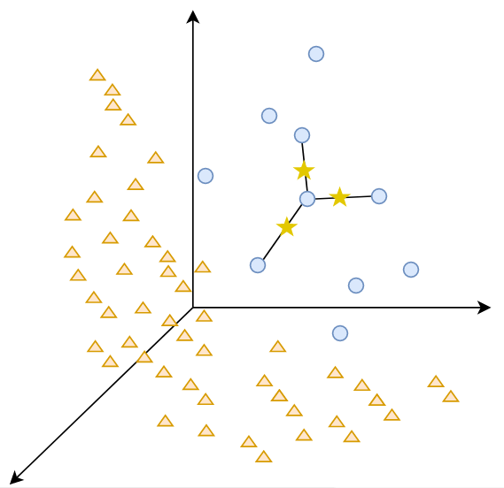
(a)

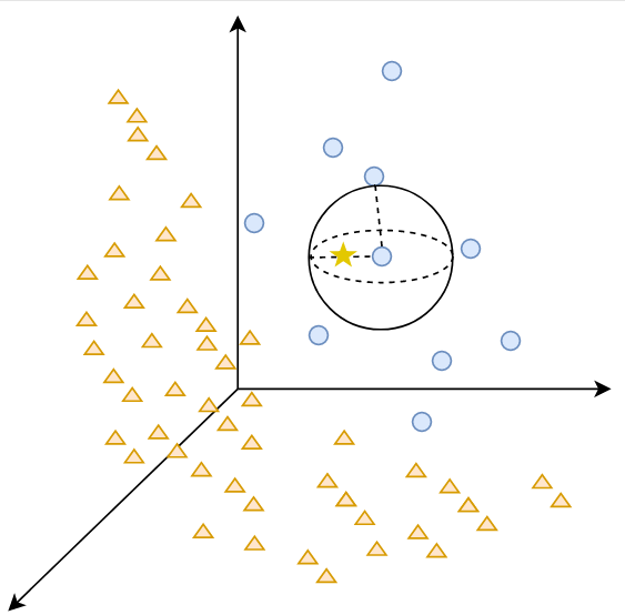
(b)

Figure 1: (a) is the illustration of SMOTE; (b) shows illustration of RSMOTE.

3 The proposed method

In this section, we will represent an improved SMOTE algorithm with appropriate sampling space for high dimensional data. Then the GMM-based synthetic sampling approach will be proposed. Afterward, an adaptive optimization method is proposed in our study for the hyperparameters of sampling process.

3.1 SMOTE in high dimensional space

To ease the presentation, some notations are established here. Suppose we have a given training dataset $S$ with $N$ cases (i.e., $|S|=N$): $S=\{(x_{i},y_{i})\},i=1,2,...,N$, in which $x_{i}\in\mathbb{R}^{1\times n}$ is an instance in the $n$-dimensional feature space $X$, $y_{i}\in\{1,2,...,C\}$ is a label associated with case $x_{i}$. In this paper, a binary classification problem is considered, i.e. $C=2$. Two subsets are defined as $S_{min}\subset S$ and $S_{maj}\subset S$, in which $S_{min}$ denotes the the set of minority class cases, and $S_{maj}$ denotes the set of majority class cases, so that $S_{min}\cup S_{maj}=S$ and $S_{min}\cap S_{maj}=\phi$.

The synthetic minority oversampling technique (SMOTE) (Chawla et al., 2002) is a typical mechanism of synthetic sampling. In this algorithm, artificial cases are drawn from a feature space similarities between the instances in $S_{min}$. Concretely, in a certain neighborhood of $x_{i}\in S_{min}$, $K$-nearest neighbors with the smallest euclidian distance between themselves and $x_{i}$ are selected to create new instances for $S_{min}$. This way can be mathematically represented as follows

$$x_{syn}=x_{i}+(x_{k}-x_{i})e$$ (1)

where $x_{k}\in S_{min}$ is one of $K$-nearest neighbors $(k=1,2,3,...,K)$ of $x_{i}$, $e$ is a random number belonging to the range of $[0,1]$, $x_{syn}$ is the new synthetic sample of minority class. According to above equation, as shown in Figure 1(a), the star point is a new sample appearing at random location of the line joining $x_{i}$ and $x_{k}$. At first glance, this sampling approaches appear to have promising benefits because it can actually use new samples to alter the balanced degree of $S_{min}$ and $S_{maj}$. However, the SMOTE degrades the sampling space to line segments joining $x_{i}$ and its $K$-nearest neighbors. In practice, it is easy to extend the sampling space to the $n$-dimensional feature space $X$. In this case, the sampling space can be represented as $\Omega_{i}=\{x_{syn}|0<|x_{syn}-x_{i}|<R\}$, where $x_{i}\in S_{min}$ is a sampling kernel, $R$ is the distance between $x_{i}$ and one of its $K$-nearest neighbors. Without loss of generality, we consider the situation of $n$=3, see Figure 1(b), synthetic samples are generated in a sphere around $x_{i}$. An illustration comparing different sampling methods with ours is given in Figure 2, in which one can see that the new synthetic samples generated by our proposed method have the more reasonable distribution in feature space $X$.

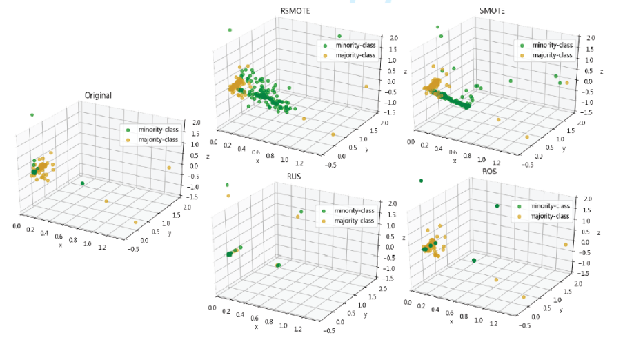
Figure 2: Comparison among RUS, ROS, SMOTE and RSMOTE on a real software engineering dataset (Core-XPConnect).

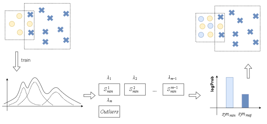
Figure 3: Entire steps of G-SMOTE.

3.2 GMM-based synthetic sampling approach

This proposed method mentioned above breaks the ties introduced by simple linear sampling space. However, there still exist two obvious drawbacks in the improved SMOTE, on one hand, this method dose not have the ability to distinguish the outliers from $S_{min}$, and huge amount of synthetic outliers could lead unfavorable performance in classification learning; on the other hand, the over generalization could increase the occurrence of overlapping between classes (Prati et al., 2004), unfortunately, there not exist detection mechanism to avoid this case in the procedure of SMOTE.

We address these problems by introducing Gaussian Mixture Model (GMM), and term this sampling method as GMM-based synthetic minority oversampling technique (GSMOTE), the entire steps of GSMOTE are illustrated in Figure fff. In the first step, the $S_{min}$ is used to train a GMM as follows

$$f(x|\mu,\Sigma)=\sum_{k=1}^{m}c_{k}\frac{1}{\sqrt{2\pi|\Sigma_{k}|}}exp[(x-\mu_{k})^{T}\Sigma^{-1}(x-\mu_{k})]$$ (2)

where $c_{k}$, $\mu_{k}$ and $\Sigma_{k}$ respectively denote weight, mean vector and variance matrix associated with the $k$th Gaussian model component, the $m$ denotes the total number of components, the training process can be completed by expectation-maximization (EM) algorithm. After a GMM is acquired, the samples in $S_{min}$ are partitioned into $m$ cliques, see Figure 3, each $c$ presents the importance degree that the corresponding clique contributes to the overall distributive characteristics of $S_{min}$. Obviously, the clique of outliers has lower importance degree than others. Thus the instances conflicting with $S_{min}$ will be selected as sampling kernel in lower probability.

In addition, the learned GMM is also employed to tackle the problem of over generalization. When a sampling kernel locates at the decision boundary, synthetic majority class instances will be generated in the sampling space . It is naturally to use the learned GMM to filter out the synthetic majority class instances. As shown in Figure 3, in this step, GMM takes all of synthetic instances as input and outputs their log probability (logprob), then top-$K$ instances with the highest logprob are selected to augment the $S_{min}$. A formal description of the GSMOTE framework is shown in Algorithm 1.

Input:

         $m$: the number of components in GMM

         $Num$: the number of selected sampling kernels

         $M$: the number of samples generated in $\Omega_{i}$

         $K$: the number of instances selected from $\Omega_{i}$

         $S_{min}$: the set of minority class cases

Output:

         $S_{syn}$: the synthetic minority class samples.

1 Create gaussian mixture model $gmm$ with $m$ components

2Train gaussian mixture model $gmm$ on $S_{min}$

3Sampling $choiced\_samples$ from $S_{min}$ based on $gmm$, and $|choiced\_samples|=Num$

4$numattr$=Number of attributes in $choiced\_samples$

5$newindex$=0

6$synthetic$=Array[$M$ $\times$ $Num$][$numattr$]

7for $i\leftarrow 0$ to $(Num-1)$ do

8       Compute $k$ nearest neighbors $nnarray$ for $choiced\_samples[i]$

9      for $j\leftarrow 0$ to $(M-1)$ do

10             random choice a case $nn$ from $nnarray$

11            $r$=distance between $choiced\_samples[i]$ and $nn$

12            Sampling a point $sample$, and distance between $sample$ and $choiced\_samples[i]$ = $d\in(0,r)$

13            $synthetic[newindex]$=$sample$

14            $newindex++$

15       end for

16      

17 end for

18

19Get the top-$K$ instances $S_{syn}$ with the highest logprob from $synthetic$

Algorithm 1 GSMOTE

3.3 An adaptive optimization method

One can see that there are several hyperparameters in the proposed GSMOTE framework. Instead of using the rules of thumb, we optimize these parameters by developing an adaptive optimization method, which is based on Differential evolution (DE). This iteratively searching process is given in following algorithm. For clear presentation, some notations are defined: the $Num$ denotes the number of sampling kernels selected in the first step, $M$ is the number of synthetic samples generated in $\Omega_{i}$, $K$ is the number of instances selected in the second step.

Table 1:

Input:

         $G$: Maximum number of generationss

         $N$: Population size

         $F$: Mutation factor

         $C_{r}$:Corssover probability

         $D$: Dimension of soultion space

         $range=(c_{min},c_{max})$: Range of values

         $S_{min}$: the set of minority class cases

Output:

         $c_{best}^{G}$

1 Generate an initial population $\{c_{1}^{0},...,c_{N}^{0}\}$.

2$c_{i}^{0}=c_{min}+rand(0,1)*(c_{max}-c_{min})$, $i=1,2,...,N$.

3Evaluate each candidate solution $c_{i}^{0}(i=1,2,...,N)$ in the initial population to obtain a vector representing the fitness functions $fitness(c_{i}^{0})$ which is accuracy of ELM on dataset augmented by Algorithm 1 in this paper. In other words, $c_{i}^{g}=(m,Num,M,K)$, $g=1,2,...,G$.

4 Function fitness($c_{i}^{g}$, $S_{min}$):

5       $(m,Num,M,K)=c_{i}^{g}$

6      $S_{syn}$= GRSMOTE($m,NUM,M,K,S_{min}$)

7      $S_{aug}$ = $S$ $\cup$ $S_{syn}$

8      train a ELM on $S_{aug}$ and calculate accuracy $acc$ on the test dataset

9      return $acc$

10      

11 return

12

13for $g\leftarrow 1$ to $G$ do

14      

15      for $i\leftarrow 1$ to $N$ do

16             Random choice three vector, $c_{r}^{1},c_{r}^{2},c_{r}^{3}$ from $(g-1)$ generation

17            $h_{i}^{g}=c_{r}^{1}+F\cdot(c_{r}^{2}-c_{r}^{3})$

18            $v_{i,j}^{g}$ = $\begin{cases}h_{i,j}^{g},&$if$\enspace rand_{j}\leq C_{r}\\ c_{i,j}^{g},&$otherwise$\end{cases}j=1,2,...,D.$

19       end for

20      if $fitness(v_{i}^{g})>fitness(c_{i}^{g-1})$ then

21             $c_{i}^{g}=v_{i}^{g}$

22      else

23             $c_{i}^{g}=c_{i}^{g-1}$

24       end if

25      

26 end for

$c_{best}^{G}=argmax(f(c_{i}^{G})),i=1,2,...,N$

Algorithm 2 Differential Evolution

4 EVALUATION ON REAL-WORLD DATASETS

4.1 Evaluation metrics

In this study, the predicted labels are defined as $\{Y,N\}$, a confusion matrix representing classification performance can be illustrated in Table 1.

Based on above table, the $accuracy$ can be defined as follows

$$Accuracy=\frac{TP+TN}{TP+TN+FP+FN}$$ (3)

which is a simple way to describe the performance of a classifier. In addition, another popular metric is $F-measure$ defined as

$$F-Measure=\frac{(1+\beta^{2})\cdot Recall\cdot Precision}{\beta^{2}\cdot Recall\cdot Precision}$$ (4)

where $\beta$ is a coefficient of importance, $Precision$ and $Recall$ respectively are

$$Precision=\frac{TP}{TP+FP}$$ (5)

$$Recall=\frac{TP}{TP+FN}$$ (6)

According to (4), we can notice that the $F$-$Measure$ is a weighted combination of $Precision$ and $Recall$, and provides insight into the functionality of a classification algorithm. Like most studies, we use an effective measure, namely $weighted$ $F$-$Measure$, to act the second metric defined as

$$w-F=\frac{n_{1}}{total}\cdot F_{1}+\frac{n_{2}}{total}\cdot F_{2}$$ (7)

where the $n_{1}$ is the num of the $class_{1}$, $n_{2}$ is the num of the $class_{2}$ and $total$ is the num of the dataset.

4.2 Experimental Result

In this section, we conduct several experiments to demonstrate the effectiveness of our proposed method. The datasets are blood, page, CVFTM. The imbalanced degree of these datasets is list in Table 2. Several classification algorithms are employed in our study, namely, j48, Naive bayes classifier(NB), Random tree(RT), Support vector machine(SVM). The experimental results are given in Table 3.

One can see that the relatively balanced datasets provided by our framework boost the performances of different classification learnings in most situations.

Table 2: The imbalanced degree of three datasets

DataSet	blood	page	CVFTM
Imbalanced Degree	3.211	8.497	4.955

Table 3:

DataSet/Measure	j48	NB	RT	SVM
boold/$Accuracy$	78	74	72	76
booldaug/$Accuracy$	78.6667	74	77.3333	76.6667
boold/$F$-$Measure$	74.4	69.7	68.9	67.5
booldaug/$F$-$Measure$	75.4	70.9	74.4	68.3
page/$Accuracy$	96.9863	90.7763	96.5297	94.3379
pageaug/$Accuracy$	97.2603	92.6941	97.3516	92.0548
page/$F$-$Measure$	97.0	90.4	96.5	93.3
pageaug/$F$-$Measure$	97.2	91.6	97.3	89.6
CVFTM/$Accuracy$	99.9537	90.1852	97.2222	99.9537
CVFTMaug/$Accuracy$	99.9537	99.9537	99.9074	99.9537
CVFTM/$F$-$Measure$	100.0	88.2	97.2	100.0
CVFTMaug/$F$-$Measure$	100.0	100.0	99.9	100.0

Besides, some experiments are conducted on bug triaging system to recognize the severity of bugs. In this situation, classification algorithms aim to distinguish $non$-$severe$ from $severe$ bugs which a software developer must fix as soon as possible. In this study, bug reports are from three major open-source projects, i.e. Eclipse (Bugzilla, 2018a), Mozilla (Bugzilla, 2018b), and Gnome (Bugzilla, 2018c). Bugzilla is the common bug tracking system used by these projects. To provide input for classification algorithms, the textual strings of report are transformed to digital vectors by the preprocessing steps which will be further described in what follows.

Tokenization.

First of all, a large textual string is divided into a group of tokens, and each of these corresponds to a single term. Meanwhile, all meaningless words (e.g. commas and punctuations) are filtered out during this process. In this step, all capitals also are replaced by corresponding lower-case letters.

Stop-words removal.

In a bug report, the stop-words, such as ‘in’, ‘that’ and ‘the’, do not include much specific contextual information, however, the frequency of these symbols are higher than others. To decrease the dimensionality and redundancy of transformed digital vectors, it is essential to remove all stop-words from each token based on the known list of stop-words.

Stemming.

In human languages, different terms commonly carry the same contextual information, and share the same morphological base, e.g., ‘computerize’ and ‘computerized’ have the same basic form: ‘computer’. To reduce the variety of descriptions, this step maps all terms with the same specific information to their common form.

Term frequency.

Based above all, a single keyword vector is extracted from a single bug report by using a keyword dictionary, and a weighting method is needed in this step, i.e. $TF\times IDF$ approach. Let $D=\{d_{1},...,d_{j},...,d_{m}\}$ denote a set of documents, in which $d_{j}=\{t_{1},...,t_{k}\}$ is a group of terms, then the term frequency ($TF_{i,j}$) of $i$th term $t_{i}$ in $j$th document $d_{j}$ can be defined as follows:

$$TF_{i,j}=\frac{rf_{i,j}}{\sum_{k}rf_{k,j}}$$ (8)

where $rf_{i,j}$ is the amount of occurrences of the $t_{i}$ $d_{j}$, and $k$ is the total number of terms in $d_{j}$. The other factor is inverse document frequency ($IDF_{i}$) representing the importance of $i$th term, which is defined as follows:

$$IDF_{i}=\log\frac{m}{df_{i}}$$ (9)

where $df_{i}$ is the document frequency, i.e. the number of documents containing $t_{i}$, $m$ is the total number of documents. The importance of a particular term will subsequently decrease when this term appears in many documents.

As discussed above, the preprocessing steps take textual strings as input and outputs keyword vectors for the next step, i.e. classification learning, in which a history of reports with known severity are the training dataset. As shown in Table 5, the experimental results show that the proposed method dose improve the performances of different classifiers in bug triaging systems.

Table 4: Bug report datasets

Num	Product	Name	Severe	Non-severe	Degree
1	GNOME	Evolution_Contacts	1071	384	2.789
2	Eclipse	CDT_cdt-core	273	66	4.136
3	Eclipse	JDT_Core	789	306	2.578
4	Moizlla	Core_Printing	702	99	7.091

Table 5:

DataSet/Measure	j48	NB	RT	SVM
1/$Accuracy$	74.089	76.289	75.739	76.289
1aug/$Accuracy$	77.113	76.770	76.632	77.388
1/$F$-$Measure$	71.245	76.799	75.402	75.646
1aug/$F$-$Measure$	75.103	77.058	75.694	77.341
2/$Accuracy$	79.941	66.667	73.451	76.991
2aug/$Accuracy$	81.416	81.711	82.301	77.581
2/$F$-$Measure$	71.554	69.263	72.208	74.455
2aug/$F$-$Measure$	76.004	76.562	79.959	76.864
3/$Accuracy$	77.443	71.963	73.516	74.247
3aug/$Accuracy$	77.991	77.443	76.073	75.151
3/$F$-$Measure$	74.113	72.827	73.049	72.166
3aug/$F$-$Measure$	76.398	76.771	73.656	73.403
4/$Accuracy$	86.642	78.527	84.894	85.893
4aug/$Accuracy$	86.642	88.764	87.016	84.401
4/$F$-$Measure$	81.586	80.890	83.456	83.046
4aug/$F$-$Measure$	81.586	84.942	85.457	81.359

References

- Bertoni et al. [2011] A. Bertoni, M. Frasca, and G. Valentini. Cosnet: a cost sensitive neural network for semi-supervised learning in graphs. In Joint European Conference on Machine Learning and Knowledge Discovery in Databases, pages 219–234. Springer, 2011.
- Bugzilla [2018a] Bugzilla. Eclipse. http://bugs.eclipse.org/bugs, 2018a. Accessed: 2018-02-02.
- Bugzilla [2018b] Bugzilla. Mozilla. http://bugzilla.mozilla.org, 2018b. Accessed: 2018-02-02.
- Bugzilla [2018c] Bugzilla. Gnome. http://bugzilla.gnome.org, 2018c. Accessed: 2018-02-02.
- Castro and Braga [2013] C. L. Castro and A. P. Braga. Novel cost-sensitive approach to improve the multilayer perceptron performance on imbalanced data. IEEE transactions on neural networks and learning systems, 24(6):888–899, 2013.
- Chan and Stolfo [1998] P. K. Chan and S. J. Stolfo. Toward scalable learning with non-uniform class and cost distributions: A case study in credit card fraud detection. In KDD, volume 98, pages 164–168, 1998.
- Chawla et al. [2004a] N. Chawla, N. Japkowicz, and A. Kotcz. Editorial: special issue on learning from imbalanced data sets. sigkdd explor newsl 6: 1–6, 2004a.
- Chawla et al. [2004b] N. Chawla, N. Japkowicz, and A. Kotcz. Editorial: special issue on learning from imbalanced data sets. sigkdd explor newsl 6: 1–6, 2004b.
- Chawla et al. [2002] N. V. Chawla, K. W. Bowyer, L. O. Hall, and W. P. Kegelmeyer. Smote: synthetic minority over-sampling technique. Journal of artificial intelligence research, 16:321–357, 2002.
- Chen and Liu [2018] C. P. Chen and Z. Liu. Broad learning system: an effective and efficient incremental learning system without the need for deep architecture. IEEE transactions on neural networks and learning systems, 29(1):10–24, 2018.
- Datta and Das [2015] S. Datta and S. Das. Near-bayesian support vector machines for imbalanced data classification with equal or unequal misclassification costs. Neural Networks, 70:39–52, 2015.
- Domingos [1999] P. Domingos. Metacost: A general method for making classifiers cost-sensitive. In Proceedings of the fifth ACM SIGKDD international conference on Knowledge discovery and data mining, pages 155–164. ACM, 1999.
- Fan et al. [1999] W. Fan, S. J. Stolfo, J. Zhang, and P. K. Chan. Adacost: misclassification cost-sensitive boosting. In Icml, pages 97–105, 1999.
- He and Garcia [2008] H. He and E. A. Garcia. Learning from imbalanced data. IEEE Transactions on Knowledge & Data Engineering, (9):1263–1284, 2008.
- Holte et al. [1989] R. C. Holte, L. Acker, B. W. Porter, et al. Concept learning and the problem of small disjuncts. In IJCAI, volume 89, pages 813–818. Citeseer, 1989.
- Japkowicz [2003] N. Japkowicz. Class imbalances: are we focusing on the right issue. In Workshop on Learning from Imbalanced Data Sets II, volume 1723, page 63, 2003.
- Japkowicz and Stephen [2002] N. Japkowicz and S. Stephen. The class imbalance problem: A systematic study. Intelligent data analysis, 6(5):429–449, 2002.
- Japkowicz et al. [2000] N. Japkowicz et al. Learning from imbalanced data sets: a comparison of various strategies. In AAAI workshop on learning from imbalanced data sets, volume 68, pages 10–15. Menlo Park, CA, 2000.
- Jo and Japkowicz [2004] T. Jo and N. Japkowicz. Class imbalances versus small disjuncts. ACM Sigkdd Explorations Newsletter, 6(1):40–49, 2004.
- Khan et al. [2017] S. H. Khan, M. Hayat, M. Bennamoun, F. A. Sohel, and R. Togneri. Cost-sensitive learning of deep feature representations from imbalanced data. IEEE transactions on neural networks and learning systems, 2017.
- Kubat et al. [1998] M. Kubat, R. C. Holte, and S. Matwin. Machine learning for the detection of oil spills in satellite radar images. Machine learning, 30(2-3):195–215, 1998.
- Lamkanfi et al. [2010] A. Lamkanfi, S. Demeyer, E. Giger, and B. Goethals. Predicting the severity of a reported bug. In Mining Software Repositories (MSR), 2010 7th IEEE Working Conference on, pages 1–10. IEEE, 2010.
- Laurikkala [2001] J. Laurikkala. Improving identification of difficult small classes by balancing class distribution. In Conference on Artificial Intelligence in Medicine in Europe, pages 63–66. Springer, 2001.
- Liu and Zhou [2006] X.-Y. Liu and Z.-H. Zhou. The influence of class imbalance on cost-sensitive learning: An empirical study. In null, pages 970–974. IEEE, 2006.
- Phua et al. [2004] C. Phua, D. Alahakoon, and V. Lee. Minority report in fraud detection: classification of skewed data. Acm sigkdd explorations newsletter, 6(1):50–59, 2004.
- Prati et al. [2004] R. C. Prati, G. E. Batista, and M. C. Monard. Class imbalances versus class overlapping: an analysis of a learning system behavior. In Mexican international conference on artificial intelligence, pages 312–321. Springer, 2004.
- Sun et al. [2007] Y. Sun, M. S. Kamel, A. K. Wong, and Y. Wang. Cost-sensitive boosting for classification of imbalanced data. Pattern Recognition, 40(12):3358–3378, 2007.
- Tang et al. [2016] J. Tang, C. Deng, and G.-B. Huang. Extreme learning machine for multilayer perceptron. IEEE transactions on neural networks and learning systems, 27(4):809–821, 2016.
- Ting [2002] K. M. Ting. An instance-weighting method to induce cost-sensitive trees. IEEE Transactions on Knowledge and Data Engineering, 14(3):659–665, 2002.
- Wang and Japkowicz [2004] B. Wang and N. Japkowicz. Imbalanced data set learning with synthetic samples. In Proc. IRIS Machine Learning Workshop, volume 19, 2004.
- Weiss [2009] G. M. Weiss. Mining with rare cases. In Data mining and knowledge discovery handbook, pages 747–757. Springer, 2009.
- Weiss and Provost [2003] G. M. Weiss and F. Provost. Learning when training data are costly: The effect of class distribution on tree induction. Journal of Artificial Intelligence Research, 19:315–354, 2003.
- Woods et al. [1993] K. S. Woods, C. C. Doss, K. W. Bowyer, J. L. Solka, C. E. Priebe, and W. P. KEGELMEYER JR. Comparative evaluation of pattern recognition techniques for detection of microcalcifications in mammography. International Journal of Pattern Recognition and Artificial Intelligence, 7(06):1417–1436, 1993.
- Yang et al. [2017] X.-L. Yang, D. Lo, X. Xia, Q. Huang, and J.-L. Sun. High-impact bug report identification with imbalanced learning strategies. Journal of Computer Science and Technology, 32(1):181–198, 2017.
- Zadrozny et al. [2003] B. Zadrozny, J. Langford, and N. Abe. Cost-sensitive learning by cost-proportionate example weighting. In Data Mining, 2003. ICDM 2003. Third IEEE International Conference on, pages 435–442. IEEE, 2003.
- Zhou and Feng [2017] Z.-H. Zhou and J. Feng. Deep forest: Towards an alternative to deep neural networks. arXiv preprint arXiv:1702.08835, 2017.
- Zhu and Wang [2017] H. Zhu and X. Wang. A cost-sensitive semi-supervised learning model based on uncertainty. Neurocomputing, 251:106–114, 2017.
- Zong et al. [2013] W. Zong, G.-B. Huang, and Y. Chen. Weighted extreme learning machine for imbalance learning. Neurocomputing, 101:229–242, 2013.