Characterisation of an n-type segmented BEGe detector

Abstract

A four-fold segmented n–type point-contact “Broad Energy” high-purity germanium detector, SegBEGe, has been characterised at the Max–Planck–Institut für Physik in Munich. The main characteristics of the detector are described and first measurements concerning the detector properties are presented. The possibility to use mirror pulses to determine source positions is discussed as well as charge losses observed close to the core contact.

1 Introduction

Germanium detectors are used in a wide variety of scientific applications [1], in fields like medicine, homeland security and applied and fundamental physics [2, 3, 4, 5]. “Broad Energy” Germanium (BEGe) detectors have become increasingly important in searches for neutrinoless double beta decay [6, 7]. The main challenge for these searches is the reduction of background. This requires as perfect an understanding of the detector properties as possible.

The segmented n-type BEGe detector presented here was designed in order to study the properties of BEGe detectors in general. One interesting subject is the influence of the crystal axes on the trajectories of the charge carriers and thus the pulse shapes. This is linked to the mobility tensors of holes and electrons. The mirror pulses, as observed in segments which do not collect charge, are an important source of information about the drifting charges inside the detector and provide spatial information. The response of BEGe detectors to interactions close to the core contact area, where charge collection inefficiencies are expected and not well understood, is another important issue. Results are presented for scans of the mantle and the end-plates of the subject detector with a ¹³³Barium source.

2 The Detector

The “SegBEGe” detector is an n-type high-purity Broad Energy Germanium (BEGe) detector, segmented as depicted in Fig. 1. It has a diameter of 75 mm and a height of 40 mm. Its specifications as provided by the producer, Mirion France, formerly Canberra France, are listed in Table 1. The side with the n⁺⁺ HV contact, i.e. the core contact, is called the top of the detector. The core contact has a diameter of 15 mm and is surrounded by a passivated ring with an outer diameter of 39 mm. The detector is four–fold segmented in $\phi$ with three individual 60-degree segments, i=1,2,3, and one segment, segment 4, combining the three other regions in $\phi$. Segment 4 is closed on the bottom end-plate, see Fig. 1. The segmentation is created through a three-dimensional implantation process. The center of the bottom plate is the origin of a cylindrical coordinate system with the $z$-axis pointing towards the core contact. The left edge of segment 1, looking from the top, defines $\phi=0$.

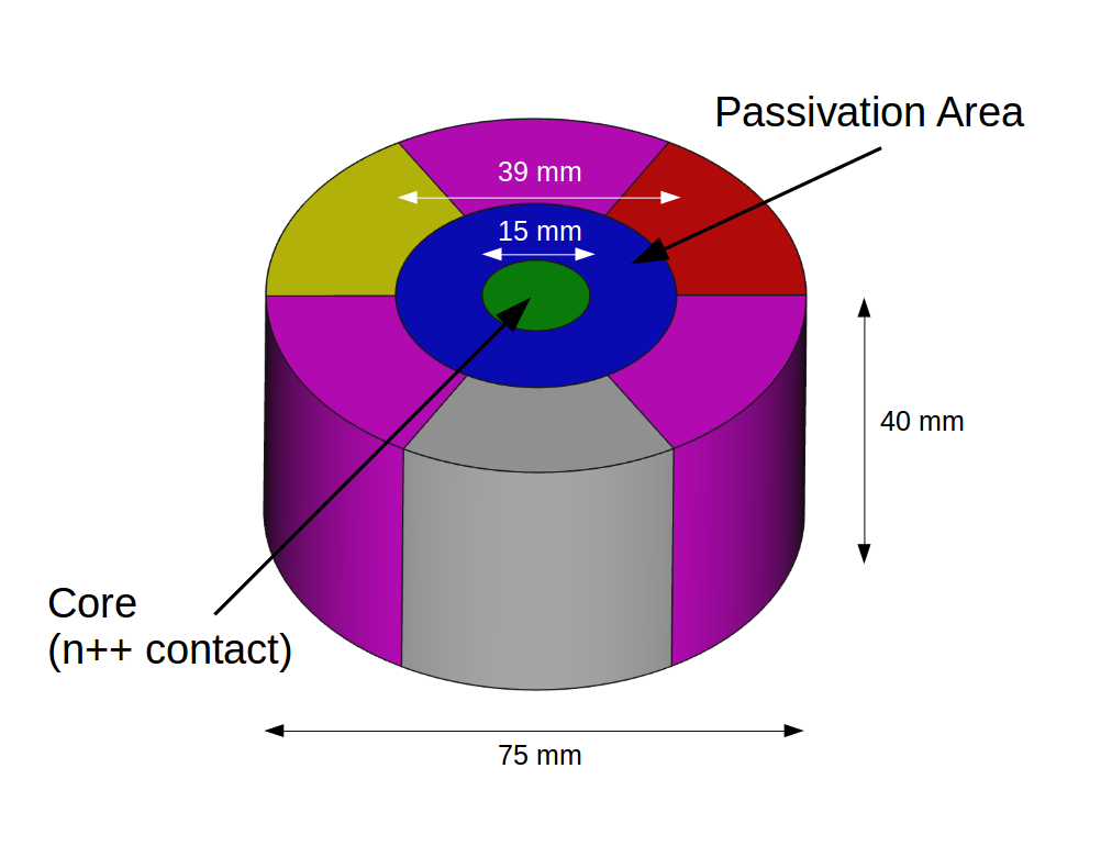
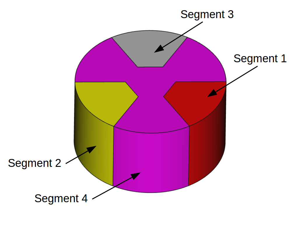
$\phi=0$

Figure 1: Schematics of the SegBEGe detector seen from the top and (left) from the bottom (right).

Parameter	Value
crystal Diameter	7.5 cm
crystal Height	4.0 cm
active Volume	177 cm3
bulk	n-type
effective impurities top	$1.3\leavevmode\nobreak\ \,\times 10^{10}/$ cm3
effective impurities bottom	$0.95\times 10^{10}/$ cm3
operating voltage	4500 V
FWHM at 122 keV
core	1.0 keV
segment 1/ 2/ 3	1.9/ 2.0/ 2.1 keV
segment 4	3.7 keV
FWHM at 1332 keV
core	4.4 keV
segment 1/ 2/ 3	3.7/ 3.8/ 4.2 keV
segment 4	5.5 keV

Table 1: Specifications of the SegBEGe detector as provided by the manufacturer.

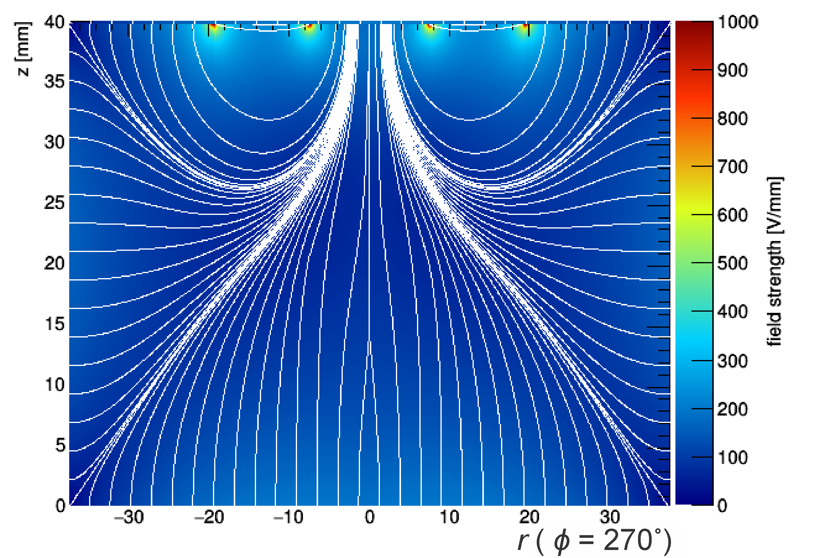
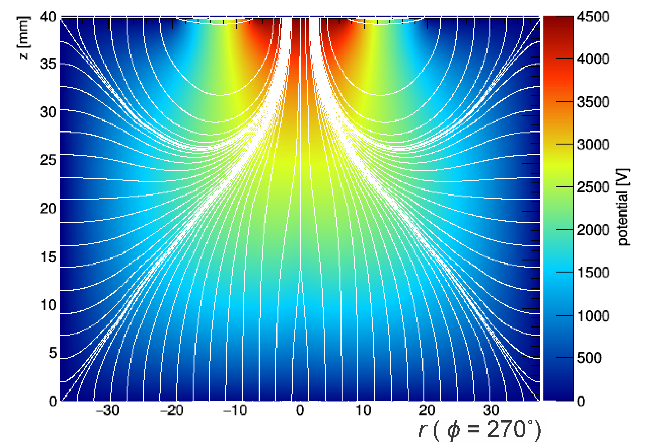
Figure 2: Electric field strength (left) and potential (right) for the $r-z$ cut through the detector at $\phi=270\degree$. Also shown are the field lines.

The electric field inside the detector is very similar to the field of an unsegmented detector. It was calculated using an upgrade to the program package described in an earlier publication [8]. The main improvements are the implementation of an adaptive grid and realistic segment boundaries. The field distortions on the mantle close to the surface around the narrow segment boundaries were found to be very shallow and insignificant for all gamma scans. The effect of the shape of the segmentation on the bottom plate on the field lines is visible in Fig. 2 which shows the electrical field strength and the potential as well as the field lines for the $r-z$ cut through the detector at $\phi=270\degree$. The slight asymmetry of the field lines seen around $r=0$ is caused by the influence of the inner boundary of segment 3. The “positive radii” in Fig. 2 indicate the cut through the middle of segment 3, the “negative radii” indicate the cut through segment 4, which also covers the centre of the bottom plate, see Fig. 1. Figure 2 is based on calculations where the width of the floating segment boundaries was assumed to be 1 mm, which is not the precise width but serves to demonstrate the influence of the segment boundaries.

The potential close to the core contact of such a detector is high. It drops rapidly, creating a strong field close to the core contact while the field close to the mantle of the detector is weak. This causes the large differences in drift speed for different regions typical for this type of detector.

The field strength at the edges of the passivated ring around the HV contact is not expected to be as high as indicated by the calculation. The calculation is based entirely on the boundary conditions for the potential which are 0 V for the segments, 4500 V for the core contact and “floating” for the passivated ring. Neither the depth of the Lithium drifted core contact nor the Lithium diffusion at the edge were implemented. Similarly, no depth or diffusion was implemented for the boron implants of the segments. Especially, the diffusion is expected to reduce the spikes in the field strength.

3 The Experimental Setup

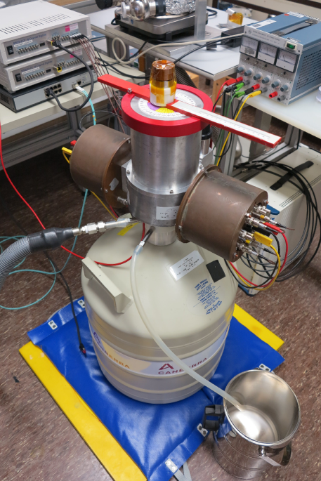
Figure 3: The experimental setup during a scan of the top of the detector during run B, figure taken from [9]. The cryostat is mounted on top of a liquid nitrogen dewar resting on a sandbag to reduce vibrations. Copper “ears” house the readout electronics. The source was positioned manually on a grid.

The detector was mounted in a conventional aluminium vacuum-cryostat called K1 for the characterisation measurements presented here. This cryostat was used previously to study the performance of the first 18-fold segmented true coaxial detector [10]. In K1, the detector is cooled through a copper finger submerged in a conventional liquid nitrogen dewar. The temperature at the top of the cooling finger was monitored using a PT100 inside the vacuum cap. Between daily refilling, the temperature was stable between 102 K and 106 K. Any influence due to changes in temperature was not corrected for in the studies presented here.

The setup is depicted in Fig. 3. The signals were amplified by PSC 823 pre-amplifiers produced by Mirion France, which were housed in the copper “ears” visible in Fig. 3. The DC-coupled room-temperature FETs for the signals of the segments were sitting on the boards of their four pre-amplifiers in one of the ears. The cold FET for the AC-coupled core signal was located inside the detector cap and was thermally coupled to the cold finger. The rest of the core pre-amplification stage was located in the other ear. The schematic of the readout is given in Fig. 4.

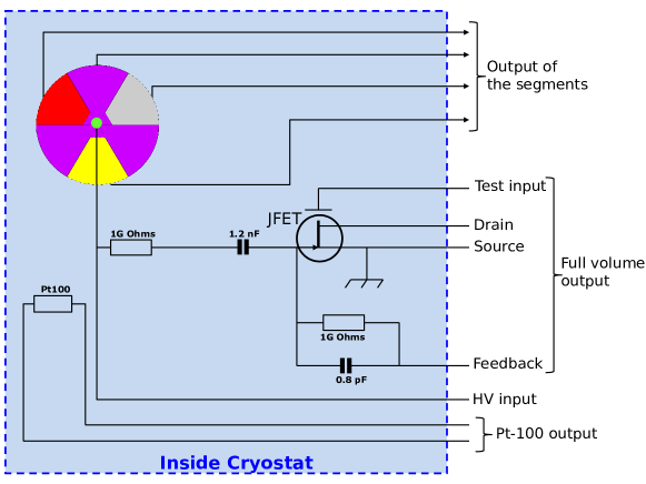
Figure 4: Schematic of the detector readout, taken from [9]. The segment signals were processed in one ear and the core (full volume) signal in the other ear.

The detector was first mounted upside down, i.e. with the core contact down; this period is called run A. For the following run B, it was mounted with the core contact up. The data acquisition systems were different for runs A and B. For run A, a PIXIE-4 system [11] with a 75 MHz sampling frequency and a 13.7 $\rm{\mu}$s trace length was used. This system used a trapezoidal filter for threshold triggering. It also provided internal pile-up suppression. For run B, a Struck 16-channel SIS3316-250-14 module [12] with a sampling frequency of 250 MHz and a trace length of 20 $\mu$s was used. This system used a trapezoidal filter with additional constant fraction time-positioning for threshold triggering. It did not provide any online suppression of saturated or pile-up events.

4 Data Taking

The detector was first commissioned in the fall of 2014. Run A lasted until summer 2015. Run B, with the detector upright, lasted from March to April 2016.

In both run periods, data were taken with an uncollimated ⁶⁰Cobalt and an uncollimated ²²⁸Thorium source to illuminate the detector bulk and study resolutions. The detector scans were performed with a ¹³³Barium source. Side-scans were performed in both runs. In run A (B), also the bottom (top) of the detector was scanned. The data sets which were used for this paper are listed in Table 2.

The gammas from the ¹³³Barium source were collimated with a 50 mm long tungsten collimator with a diameter of 35 mm and a 1 mm radius collimation hole. A purely geometrical calculation shows that the beam spots on the detector surface had radii of 2.9 mm on the side and 2.6 mm on the end-plates.

Label	Type	Source	Beam Spot	$z$	$r$	$\phi$
Co-B	bulk	60Co	n/a	on top of	$r$=0	n/a
Th-B	bulk	228Th	n/a	cryostat	$r$=0	n/a
Bsc	bottom-scan	133Ba	2.6 mm	$z$=0 mm	$r$=25.0 mm	0 – 360 o
Ssc-A	side-scan	133Ba	2.9 mm	$z$=20 mm	$r$=37.5 mm	0 – 360 o
Ssc-B	side-scan	133Ba	2.9 mm	$z$=20 mm	$r$=37.5 mm	0 – 360 o
Tsc	top-scans	133Ba	2.6 mm	$z$=40 mm	$r$=30,18,	0 – 360 o
					13,9,6 mm

Table 2: Data sets used for this paper. The values listed under beam spot are the beam spot radii on the detector surface. The $z$, $r$ and $\phi$ values listed are in detector coordinates. The $z$ and $r$ values were adjusted to $\pm$ 0.5 mm, $\phi$ was controlled to $\pm$ 1 degree.

5 Data Processing

The online energy determination provided by the PIXIE system in run A was not used for the results presented here. However, the PIXIE system suppressed pile-up and saturated events online while the Struck system was not programmed to suppress such events. For run B, events from pile-up and saturation were suppressed by evaluating the slopes of the baseline and the decay-corrected signal plateau. A negative baseline slope indicates pile-up and a positive plateau slope indicates saturation. During Barium scans, a total of about 5 % of the events were rejected. These were dominated by events with a saturated amplifier. Actual pile-up was at the level of about 1 %.

The rest of the offline data processing was identical for both runs. The recorded raw pulses were baseline subtracted and corrected for the pre-amplifier specific decay of the pulses [9, 13]. Signal amplitudes were derived using a fixed-size window filter, where the position of the window was determined by the trigger. For run A (B), a baseline window of 4.48 $\mu$s (8.0 $\mu$) and an amplitude window of 6.63 $\mu$s (9.0 $\mu$) were chosen. This filter introduces the least bias with respect to different pulse shapes. The baseline and amplitude windows were separated far enough to ensure that the actual rise of the pulse started after the baseline and ended before the amplitude window.

Cross-talk effects between the core and the segments as well as between segments were treated in an automated calibration procedure using single-segment events [9, 13]. A calibration was performed for each data set individually. The cross-talk correction was performed under the assumption that the cross-talk from all segments to the core was identical. This assumption affected the core energy scale for single-segment events in different segments by less than 0.1 % [9, 13]. In effect, this insignificantly worsens the core energy resolution and does not affect any aspect of the analysis. The cross-talk from one particular segment to another segment is always measured together with the cross-talk from the core to this segment. Segment 4 events resulted in a cross-talk of $1\sim 2$ % into the small segments 1,2 and 3 while events in these small segments caused a cross-talk of about 0.4 % into the large segment 4.

6 Overall Detector Performance

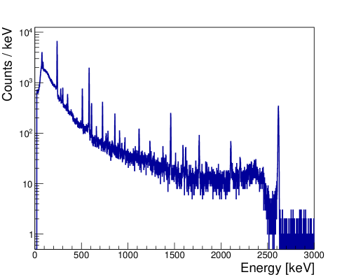
Figure 5: Core spectrum from a 1-hour Th-B data set.

		FWHM [keV]
Source	$\gamma$-line [keV]	Core	Seg. 1	Seg. 2	Seg. 3	Seg. 4
133Ba	81	3.29	5.15	4.05	4.07	7.26
	356	2.64	4.58	3.47	3.52	6.04
60Co	1173	4.57	4.88	4.16	4.34	8.05
	1332	4.93	5.00	4.39	4.14	7.84
228Th	2614	7.65

Table 3: Energy resolutions as absolute FWHMs in keV for the core and all segments as observed in run B.

The detector performed as expected in the K1 cryostat. The conditions in this setup were not perfect with respect to grounding and shielding. Thus, the resolutions were a bit worse than listed by the manufacturer. Results from run B are listed in Table 3. The lack of energy dependence for the resolutions demonstrates that the results are dominated by electronic noise. However, the detector resolution did not affect any of the results presented here. Figure 5 shows the core spectrum for a 1-hour Th-B data set. The 2614 keV ²⁰⁸Tl line is clearly visible as well as the ²¹²Bi lines at 239 and 1620 keV. In addition, the natural background in the laboratory features the usual lines from the uranium decay chain as well as a strong 1460 keV line from ⁴⁰K.

The double-escape peak from the 2614 keV Thallium line at 1592 keV and the 1620 keV Bismuth line were used for a standard pulse-shape analysis to show that the segmentation did not affect the core pulses. The Bismuth line is dominated by multi-site events from Compton scattering. The double-escape peak is dominated by single-site events; in these events all the energy is deposited in one small volume. The so-called A/E-method uses as a discriminator the ratio of A, the maximum of the first derivative of a pulse, i.e. the maximum current, divided by the total energy of the event. The method was applied to Th-B data [9]. For a survival probability of the double-escape peak of 90 %, a reduction of the Bismuth peak of 86 % was obtained. That is compatible with the results obtained for other BEGe detectors [6, 14].

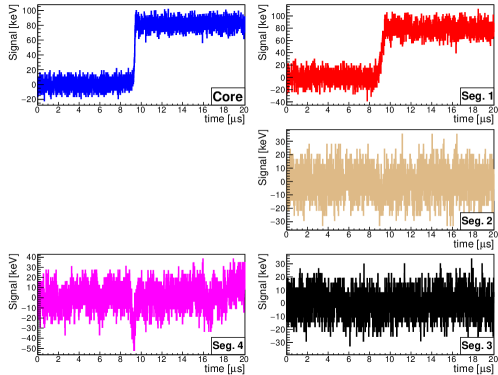
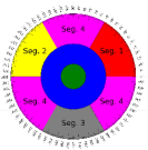
Figure 6: Single 81 keV event from the Ssc-B data set for $\phi=45^{\circ}$. The core pulse is shown at the top left, segments 1,2,3 are shown from top to bottom on the right and segment 4 is shown at the bottom left. The inset depicts the detector top with a $\phi$ scale.

7 Super-pulses

The 81 keV line from ¹³³Ba was chosen as the line for which scanning results are presented. The gammas from this line have a penetration depth of about 1.8 mm and thus create events very close to the surface. As a result, the holes are collected quickly and the drift is dominated by electrons. A single event at 81 keV as recorded in the Ssc-B data set at $\phi=45^{\circ}$ is shown in Fig. 6.

The event was located on the surface of segment 1. The largest mirror pulse is expected in segment 4 next to the collecting segment 1. It is clearly visible in Fig. 6. Smaller mirror pulses are expected in segments 2 and  3. The noise level is such that they cannot be easily identified in individual events. As the S/N ratio was 10 or more for this line and the pulses are all very similar due to the low penetration power of the 81 keV gammas, the pulses in 10 keV intervals around the peaks were averaged to form super-pulses for each position. Typically, 2000 to 2500 pulses were averaged. The super-pulse for the location of the event depicted in Fig. 6 is shown in Fig. 7. The super-pulse also clearly reveals the smaller mirror pulses in segments 2 and 3. As the noise gets averaged out super-pulses are a powerful tool to investigate detector properties.

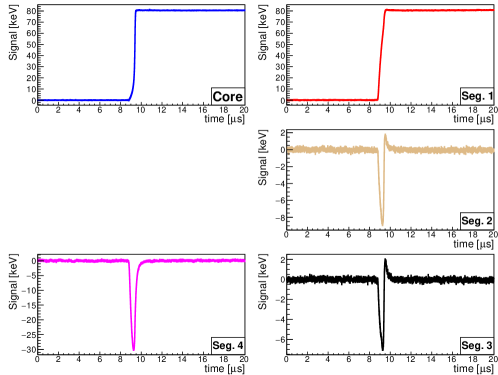
Figure 7: Super-pulse for 81 keV events from the Ssc-B data set for $\phi=45^{\circ}$. The core super-pulse is shown at the top left, segments 1,2,3 are shown from top to bottom on the right and segment 4 is shown at the bottom left. Please note the different scales used for the different segments. The inset depicts the detector top with a $\phi$ scale.

8 Segment Boundaries

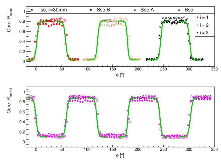
Figure 8: Ratios $R_{ss_{i}/all}$ for (top) the three individual segments i=1,2,3 and (bottom) the large segment 4. Shown are data for run A (open symbols) and run B (full symbols). Also shown are fits of the function in Eq. 1 to the Tsc data from run B.

The segment boundaries were determined using the rate of single-segment events in the respective bottom-, side- and top-scans. The ratios, $R_{ss_{i}/all}$, of the number of single-segment events in segment $i$ with $i\in[1,2,3,4]$ over all single-segment events were used. A value close to one is expected if the source is facing the respective segment, close to zero, depending on the background level, is expected otherwise. The data as obtained for the 81 keV line from ¹³³Ba in the Bsc, Ssc-A/B and Tsc scans are depicted in Fig. 8. Segment 4 has a higher background level due to its larger volume. The side-scans were affected by some parts of the detector holder, reducing the event numbers in the middle of some segments. Also shown are the results of fits to the Tsc data using the function:

$$R_{ssi/all}(\phi)=\frac{H}{2}\cdot\tanh[\Lambda\cdot(\phi-\phi_{i,j})]+\Gamma\leavevmode\nobreak\ \leavevmode\nobreak\ \leavevmode\nobreak\ ,$$ (1)

where the four fitted parameters are

• $H$: the maximal variation in $R_{ssi/all}$,

• $\Lambda$: the slope of the variation in $R_{ssi/all}$: $\Lambda>(<)\leavevmode\nobreak\ 0$ for rising (falling) edges,

• $\phi_{i,j}$: the boundary between segments $i$ and $j$,

• $\Gamma$: the source location independent background.

The segment boundaries were found consistently in all scans during both run periods. The information was mainly used to have precise location information on the detector.

9 Crystal Axes

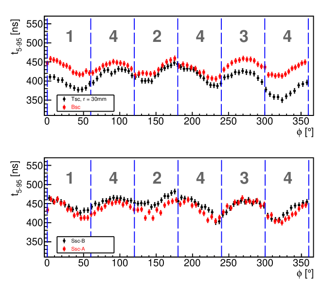
Figure 9: Average 5 $\%$ to 95 $\%$ rise-times of 81 keV super-pulses as a function of the azimuth angle $\phi$ for (bottom) the two side-scans from runs A and B and (top) the bottom and top-scans from runs A and B. The error bars represent an uncertainty corresponding to a temperature shift of roughly 2 K.

The propagation of electrons and holes in the electric field of the germanium crystal is influenced by the crystal axes [15]. The charge carriers get deflected and do not follow a simple radial path. Thus, the time to collect the charge carriers depends on the angle between the closest crystal axis and the radial line on which the interaction takes place. For a perfect crystal in a perfect setup, a sine function is expected:

$$t_{5-95}=C+a\cdot\sin\left[\frac{2\pi}{90}\left(\phi+\phi_{\rm offset}\right)\right]\leavevmode\nobreak\ \leavevmode\nobreak\ \leavevmode\nobreak\ ,$$ (2)

where $t_{5-95}$ is the time a pulse needs to rise from 5 % to 95 % of its amplitude, $C$ is the mean $t_{5-95}$ and $a$ the amplitude of the variation of $t_{5-95}$. The parameter $\phi_{\rm offset}$ is fitted to determine the location of the axes.

The data using 81 keV super-pulses are shown in Fig. 9 for scan data from both run A and B. The data from the different periods and scans agree well. However, the scan data were affected by a small tilt of the detector that caused a shift of the impact points with respect to the detector coordinates. This effect was not corrected for. The top-scan was affected the most. The smaller radius at which the bottom-scan was performed limited this effect for the bottom-scan. The error bars shown in Fig. 9 represent the uncertainty due to changes in the temperature, which was not controlled to better than $\pm$ 2 K.

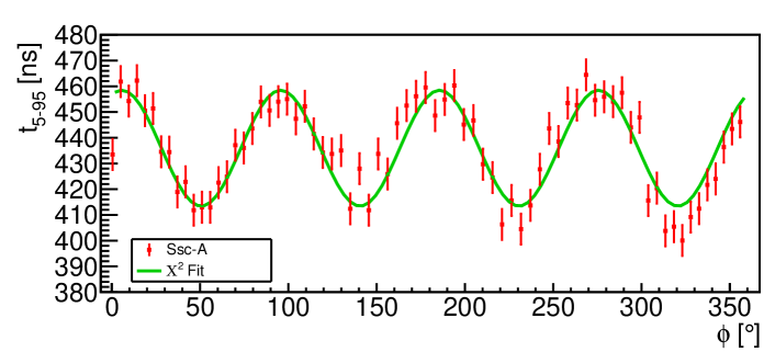
Figure 10: Average 5 $\%$ to 95 $\%$ rise-times of 81 keV super-pulses from Ssc-A together with a fit according to Eq. 2.

The side-scan data from run A are shown together with a fit according to Eq. 2 in Fig. 10. The sine function describes the data well. The $\phi$ values for which the drift-time is maximal indicate the so-called “slow axes”. The axes with minimal drift-time are called “fast axes”. The difference between drift-times will, in the future, be compared to simulation results to study the mobility of electrons.

10 Position Reconstruction

The electrons and holes drifting to the electrodes of the collecting segment create mirror charges in the neighboring segments. These mirror pulses end at the baseline once the charge carriers are collected at the electrodes. This phenomenon can be understood and deduced from Ramo’s theorem. The amplitudes, MA_i for segments $i=1,2,3,4$, defined as the maximum of the absolute values, and shapes of the induced mirror pulses depend on the location of the interaction point which determines the drift paths of the charge carriers. The closer a drifting charge passes a neighbouring segment $k$, the larger MA_k becomes.

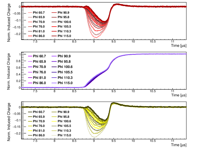
segment 1
                                                                              segment 4
                                                                              segment 2

Figure 11: From top to bottom: The super-pulses in segments 1,4,2 from the data set Ssc-B in the range $60^{o}<\phi<120^{o}$ for the 81 keV line, adapted from [9]. All pulses are normalised to an amplitude of 1 in the collecting segment 4.

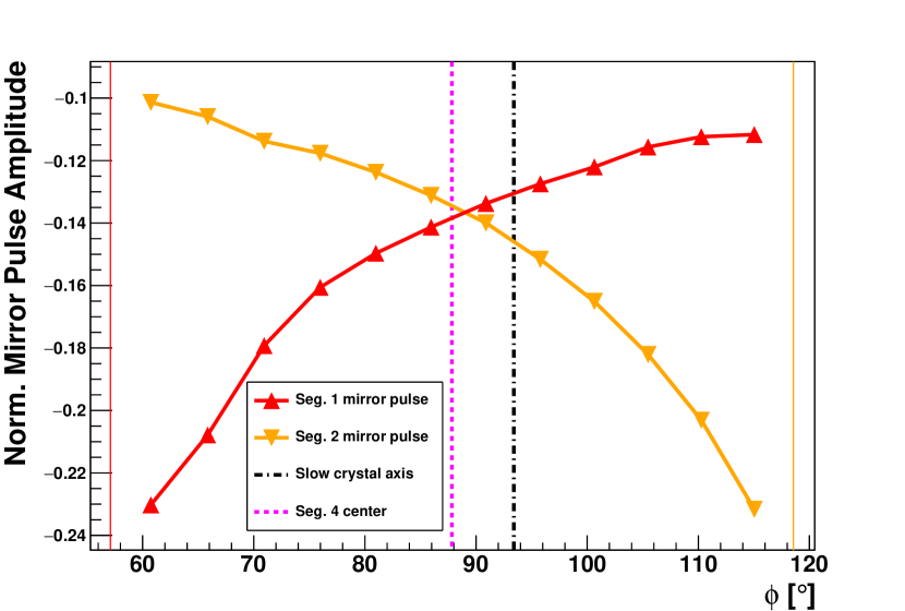
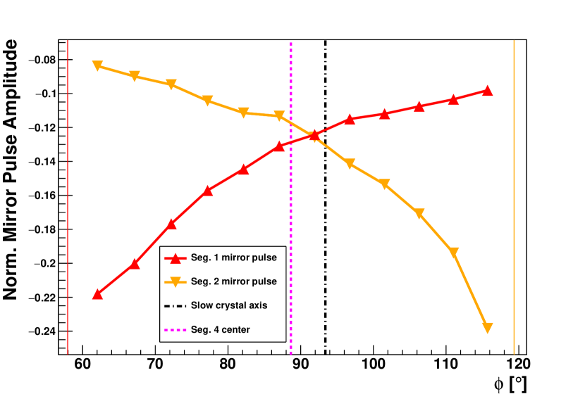
Figure 12: The mirror pulse amplitudes of the 81 keV super-pulses for the Ssc-B (left) and Tsc (right) scans for the area of segment 4 between segment 1 and segment 2. Also indicated are the segment boundaries (solid vertical lines), the centre of segment 4 (dotted vertical line) and the location of the slow axis (dashed-dotted vertical line). The data points are connected with straight lines to guide the eye.

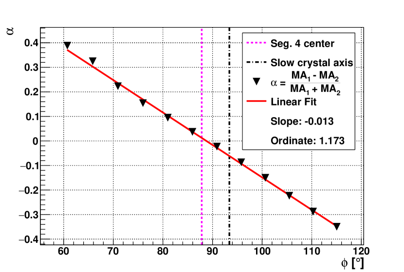
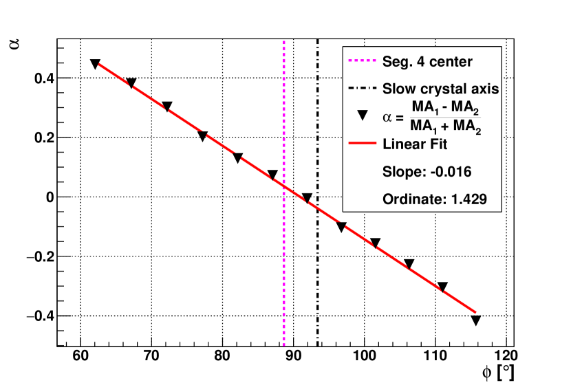
Figure 13: The asymmetries of mirror pulse amplitudes of the super-pulses for the Ssc-B (left) and Tsc (right) scans for the area of segment 4 between segment 1 and segment 2. Also shown are linear fits to the data.

The part of segment 4 between segments 1 and 2 was chosen to investigate the phenomenon. The super-pulses from the 81 keV line for $60^{o}<\phi<120^{o}$ from the Ssc-B data set are shown in Fig. 11 for the segments 1,4,2. The mirror pulses are all negative because only the drift of the electrons is seen. The MA values of the pulses decrease for segment 1 as the source moves away towards segment 2. At the same time the MA values increase in segment 2. Both segments also show that not only the amplitude of the mirror pulse changes but also the time at which the amplitude is reached. The pulse in the collecting segment 4 only changes moderately. This moderate change is due to the influence of the slow axis which is contained in that sector of segment 4.

The amplitudes, MA₁ and MA₂, of the pulses depicted in Fig. 11 are shown in the left panel of Fig. 12. The right panel depicts equivalent data from the top-scan Tsc. Also indicated in the figure are the segment boundaries, the centre of segment 4 and the location of the slow axis. Due to the influence of the slow axis, the cross-over point between the two segment amplitudes is not at the segment centre. Trajectories are bent towards the slow axis and thus the cross-over point is pulled towards the slow axis. The effect is larger for the Tsc data because from $z=40$ mm and $r=30$ mm the inwards drift affected by the slow axis passes through a relatively low field a bit longer than for the Ssc-B data at $z=20$ mm and $r=37.5$ mm.

In order to reconstruct the position of the source, a simple asymmetry, $\alpha$, was used:

$$\alpha=\frac{MA_{1}-MA_{2}}{MA_{1}+MA_{2}}\leavevmode\nobreak\ \leavevmode\nobreak\ .$$ (3)

The asymmetries for the mirror pulse amplitudes together with linear fits are shown in Fig. 13. There was no attempt made to provide statistical or $a\leavevmode\nobreak\ priori$ systematical uncertainties. The linear fits are quite good. However, they provide different slopes and ordinates. The charge carrier trajectories are very different for side and top-scans. Considering this, the differences are expected. In general, the trajectories are very dependent on the $z$-position for side-scans and $r$-position for top-scans. Thus, a simple asymmetry like $\alpha$ can only reconstruct the $\phi$ of surface events to about 10 degrees [9] if there is no information on $z$ ($r$) available.

11 Charge Losses around the Core Contact

The core contact and the surrounding passivation ring were investigated especially to look for possible charge losses. The core spectra for selected irradiation points at different radii are shown in Fig. 14.

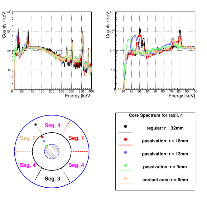
Figure 14: The core spectra for top-scan locations on the contact, the passivation ring and the “regular” area of the detector, adapted from [9]. The spectra are shown from 10 to 400 keV in the top left and from 10 to 100 keV in the top right. The spectra are coloured (shaded) according to the legend. The scan locations are shown in the bottom left.

The reference spectrum at $r=$ 32 mm shows the expected peak at 81 keV and the double peak at 31 keV and 35 keV from the ¹³³Ba source. In addition, higher energy lines are shown. As soon as part of the beam spot reaches the passivation ring, part of the events show a reduced energy. For the source locations where the beam spot is fully contained on the passivation ring, all events show a reduced energy. When part of the beam spot illuminates the core contact some events are again observed at the nominal energy of 81 keV. The effect of the passivation ring is even stronger for the 31 keV and 35 keV lines. These photons have even less penetration power than the 81 keV photons and, thus, it is not surprising that they are affected more. It is noteworthy that these 31 keV and 35 keV peaks cannot be observed when the beam spot illuminates the core contact which is Lithium drifted.

The higher energy lines are also affected. They show pronounced low-energy shoulders which are caused by events with a shallow interaction point. However, for most events the expected energy is recorded.

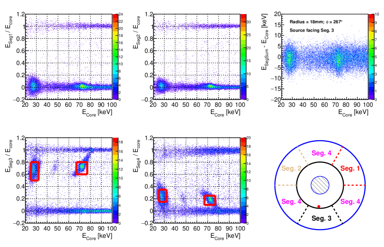
Figure 15: Distributions of the ratios of segment energies, $E_{\rm Seg\,i}$, divided by the core energy $E_{\rm core}$ vs. $E_{\rm core}$ for $i=1$ to 4 in the four left panels. The top right panel shows the difference between $\sum E_{\rm Seg\,i}$ and $E_{\rm core}$ vs. $E_{\rm core}$. The graphic at the bottom right indicates the source position.

The behaviour as observed in Fig. 14 was the same for a given $r$, independent of $\phi$. Figure 15 provides information on the segment energies for individual events for a beam spot partially illuminating the outer edge of the passivation ring. Even though gammas in the beam spot deposited their energy very close to segment 3, all segments show events where the charge is actually collected in these segments. For these events, $E_{\rm Seg\,i}/E_{\rm core}\approx 1$. Most of them can be associated with background. The relevant features are observed in segments 3 and 4. Part of the deposited charge is not collected in segment 3, but in segment 4. This is clearly visible for the 81 keV line and the effect is stronger for the 31 keV and 35 keV lines. This indicates that the drift paths right underneath the passivation ring are irregular and that possibly a surface channel forms. The charge loss observed in the core is also observed in the sum of segment energies.

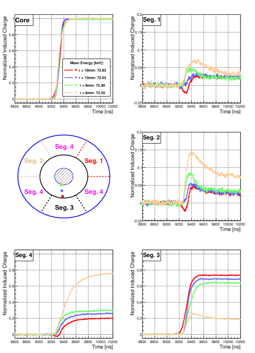
Figure 16: Super-pulses for 81 keV events as indicated by the small boxes in Fig. 15. The top left panel depicts core pulses, segments 1 to 3 are shown from top to bottom on the right, segment 4 pulses are depicted on the bottom left. The graphic at the centre left indicates the source positions. Source positions and line appearance are matched in colour (shading).

The events within the red boxes were identified as events with charge losses and super-pulses of these events were formed. Such super-pulses for the core and all segments for different radii are shown in Fig. 16. They provide some insight on what happens for interactions underneath the passivation layer.

For interaction points underneath the passivation ring or contact, the holes are not immediately absorbed like underneath a segment but have to drift a considerable distance. As the interaction points move towards the core contact this hole drift becomes longer and longer. As a result, charge is also collected in segment 4 and the mirror pulses in segments 2 and 3 become positive. The charge collected in segment 3 drops steadily while the charge collected in segment 4 increases. Already at the centre of the ring, more energy is collected in segment 4 which is considerably larger and has a larger capacitance.

Even for the source position close to segment 3, the mirror pulses in segments 1 and 2 turn positive after the fast drift of the electrons towards the core contact has ended. This indicates that the holes drift much slower in this region than the electrons. In addition, some holes are pulled towards segment 4 and thus come closer to segments 1 and 2. The core pulses are only slightly affected because the weighting potential for the core drops quickly for increasing $r$.

The positive mirror pulses in segments 1 and 2 do not return to the baseline. This indicates that at least part of the holes are trapped and do not reach any segment electrode. This creates the charge loss. When adding the mirror pulse amplitudes to the collected charges, the line energy is roughly recovered. These observations hint at the formation of a surface channel where holes drift very slowly right underneath the passivation layer and have a finite probability to get trapped.

12 Summary and Outlook

A four–fold $\phi$-segmented n-type BEGe detector was tested extensively at the “Max-Planck-Institut für Physik” in Munich. The segmentation did not influence the detector performance as measured through the core contact. The result of an A/E pulse-shape analysis was compatible with the results obtained for standard BEGe detectors.

The location of detector segments and crystal axes could be reliably established through low-energy gamma surface scans using super-pulses. Mirror pulses in non-collecting segments were investigated and their super-pulses were used to reconstruct the $\phi$ position of the interactions of low-energy gammas. Mirror pulses were also used to investigate charge losses underneath the core contact and the passivation ring. They can be attributed to low fields, surface channel effects and trapped holes.

After the series of measurements presented here, the detector was mounted in a temperature controlled cryostat. The influence of the temperature on the drift speed along different axes will be studied using detailed pulse-shape information. The super-pulses from the collecting segment 4 as shown in Fig. 11 clearly reveal the different drift zones in the detector. The electrons drift inwards first and then reach the high field zone and are pulled upwards to the contact. This allows the separation of drift times along different axes and, thus, a detailed study of the mobility tensor depending on all three crystallographic axes. In addition, the temperature dependence of the observed charge losses will be investigated.

Segmentation is an excellent tool to study detector properties. The detector presented here is based on an n-type crystal. A similar detector based on a p-type crystal is currently under construction.

Bibliography

Bibliography

-
[1]
K. Vetter, Recent
developments in the fabrication and operation of germanium detectors, Annual
Review of Nuclear and Particle Science 57 (1) (2007) 363–404.
arXiv:https://doi.org/10.1146/annurev.nucl.56.080805.140525, doi:10.1146/annurev.nucl.56.080805.140525.
URL https://doi.org/10.1146/annurev.nucl.56.080805.140525 - [2] S. Akkoyun, et al., AGATA – Advanced Gamma Tracking Array, Nucl. Instr. and Meth. A 668 (2012) 26. arXiv:1111.5731v2, doi:10.1016/j.nima.2011.11.081.
- [3] N. Abgrall, et al., The Majorana Demonstrator Neutrinoless Double-Beta Decay Experiment, Adv. High Energy Phys. 2014 (2014) 365432. arXiv:1308.1633, doi:10.1155/2014/365432.
-
[4]
K.-H. Ackermann, et al.,
The GERDA experiment
for the search of 0 decay in 76Ge, Eur. Phys. J. C
73 (3) (2013) 2330.
doi:10.1140/epjc/s10052-013-2330-0.
URL https://doi.org/10.1140/epjc/s10052-013-2330-0 - [5] C. Aalseth, et al., CoGeNT: A Search for Low-Mass Dark Matter using p-type Point Contact Germanium Detectors, Phys. Rev. D88 (1) (2013) 012002. arXiv:1208.5737, doi:10.1103/PhysRevD.88.012002.
-
[6]
M. Agostini, et al.,
Production,
characterization and operation of 76 Ge enriched BEGe detectors in GERDA,
Eur. Phys. J. C 75 (2) (2015) 39.
doi:10.1140/epjc/s10052-014-3253-0.
URL https://doi.org/10.1140/epjc/s10052-014-3253-0 - [7] S. Mertens, et al., MAJORANA Collaboration’s Experience with Germanium Detectors, Journal of Physics: Conference Series 606 (2015) 012005. doi:10.1088/1742-6596/606/1/012005.
-
[8]
I. Abt, et al., Pulse
shape simulation for segmented true-coaxial HPGe detectors, Eur. Phys. J.
C 68 (3-4) (2010) 609.
doi:10.1140/epjc/s10052-010-1364-9.
URL https://doi.org/10.1140/epjc/s10052-010-1364-9 -
[9]
M. Schuster,
Characterization
of a segmented n-type broad energy germanium detector, Master’s thesis,
Technische Universität München (2017).
URL https://wwwgedet.mpp.mpg.de/publication/Schuster_MasterThesis.pdf -
[10]
I. Abt, et al.,
Characterization
of the first true coaxial 18-fold segmented n-type prototype HPGe detector
for the GERDA project, Nucl. Inst. and Meth. A 577 (2007) 574.
doi:http://dx.doi.org/10.1016/j.nima.2007.03.035.
URL http://www.sciencedirect.com/science/article/pii/S0168900207005566 - [11] XIA, Manual: 4-Channel 75 MHz PXI Digital Spectrometer (2013).
-
[12]
Struck Innovative Systeme GMBH,
SIS3316 Family 16 Channel
VME Digitizer (2014).
URL http://www.struck.de/sis3316-2014-03-20.pdf -
[13]
L. Hauertmann,
Influence
of the Metallization on the Charge Collection Efficiency of Segmented
Germanium Detectors, Master’s thesis, Technische Universität
München (2017).
URL https://wwwgedet.mpp.mpg.de/publication/thesis_final_20170330_compressed.pdf -
[14]
H.-Y. Liao,
Development of pulse
shape discrimination methods for BEGe detectors, Ph.D. thesis,
Ludwig-Maximilians-Universität München (2016).
URL http://nbn-resolving.de/urn:nbn:de:bvb:19-195195 - [15] H. G. Reik, H. Risken, Drift velocity and anisotropy of hot electrons in n germanium, Phys. Let. 126 (1962) 1737. doi:doi.org/10.1103/PhysRev.126.1737.