Active Ranking with Subset-wise Preferences

Abstract

We consider the problem of probably approximately correct (PAC) ranking $n$ items by adaptively eliciting subset-wise preference feedback. At each round, the learner chooses a subset of $k$ items and observes stochastic feedback indicating preference information of the winner (most preferred) item of the chosen subset drawn according to a Plackett-Luce (PL) subset choice model unknown a priori. The objective is to identify an $\epsilon$-optimal ranking of the $n$ items with probability at least $1-\delta$. When the feedback in each subset round is a single Plackett-Luce-sampled item, we show $(\epsilon,\delta)$-PAC algorithms with a sample complexity of $O\left(\frac{n}{\epsilon^{2}}\ln\frac{n}{\delta}\right)$ rounds, which we establish as being order-optimal by exhibiting a matching sample complexity lower bound of $\Omega\left(\frac{n}{\epsilon^{2}}\ln\frac{n}{\delta}\right)$—this shows that there is essentially no improvement possible from the pairwise comparisons setting ($k=2$). When, however, it is possible to elicit top-$m$ ($\leq k$) ranking feedback according to the PL model from each adaptively chosen subset of size $k$, we show that an $(\epsilon,\delta)$-PAC ranking sample complexity of $O\left(\frac{n}{m\epsilon^{2}}\ln\frac{n}{\delta}\right)$ is achievable with explicit algorithms, which represents an $m$-wise reduction in sample complexity compared to the pairwise case. This again turns out to be order-wise unimprovable across the class of symmetric ranking algorithms. Our algorithms rely on a novel pivot trick to maintain only $n$ itemwise score estimates, unlike $O(n^{2})$ pairwise score estimates that has been used in prior work. We report results of numerical experiments that corroborate our findings.

1 Introduction

Ranking or sorting is a classic search problem and basic algorithmic primitive in computer science. Perhaps the simplest and most well-studied ranking problem is using (noisy) pairwise comparisons, which started from the work of Feige et al. (1994), and which has recently been studied in machine learning under the rubric of ranking in ‘dueling bandits’ (Busa-Fekete and Hüllermeier, 2014).

However, more general subset-wise preference feedback arises naturally in application domains where there is flexibility to learn by eliciting preference information from among a set of offerings, rather than by just asking for a pairwise comparison. For instance, web search and recommender systems applications typically involve users expressing preferences by clicking on one result (or a few results) from a presented set. Medical surveys, adaptive tutoring systems and multi-player sports/games are other domains where subsets of questions, problem set assignments and tournaments, respectively, can be carefully crafted to learn users’ relative preferences by subset-wise feedback.

In this paper, we explore active, probably approximately correct (PAC) ranking of $n$ items using subset-wise, preference information. We assume that upon choosing a subset of $k\geq 2$ items, the learner receives preference feedback about the subset according to the well-known Plackett-Luce (PL) probability model (Marden, 1996). The learner faces the goal of returning a near-correct ranking of all items, with respect to a tolerance parameter $\epsilon$ on the items’ PL weights, with probability at least $1-\delta$ of correctness, after as few subset comparison rounds as possible. In this context, we make the following contributions:

1. We consider active ranking with winner information feedback, where the learner, upon playing a subset $S_{t}\subseteq[n]$ of exactly $k=|S_{t}|$ elements at each round $t$, receives as feedback a single winner sampled from the Plackett-Luce probability distribution on the elements of $S_{t}$. We design two $(\epsilon,\delta)$-PAC algorithms for this problem (Section 5) with sample complexity $O\left(\frac{n}{\epsilon^{2}}\ln\frac{n}{\delta}\right)$ rounds, for learning a near-correct ranking on the items.

2. We show a matching lower bound of $\Omega\left(\frac{n}{\epsilon^{2}}\ln\frac{n}{\delta}\right)$ rounds on the $(\epsilon,\delta)$-PAC sample complexity of ranking with winner information feedback (Section 6), which is also of the same order as that for the dueling bandit ($k=2$) (Yue and Joachims, 2011). This implies that despite the increased flexibility of playing larger sets, with just winner information feedback, one cannot hope for a faster rate of learning than in the case of pairwise comparisons.

3. In the setting where it is possible to obtain ‘top-rank’ feedback – an ordered list of $m\leq k$ items sampled from the Plackett-Luce distribution on the chosen subset – we show that natural generalizations of the winner-feedback algorithms above achieve $(\epsilon,\delta)$-PAC sample complexity of $O\left(\frac{n}{m\epsilon^{2}}\ln\frac{n}{\delta}\right)$ rounds (Section 7), which is a significant improvement over the case of only winner information feedback. We show that this is order-wise tight by exhibiting a matching $\Omega\left(\frac{n}{m\epsilon^{2}}\ln\frac{n}{\delta}\right)$ lower bound on the sample complexity across $(\epsilon,\delta)$-PAC algorithms.

4. We report numerical results to show the performance of the proposed algorithms on synthetic environments (Section 8).

By way of techniques, the PAC algorithms we develop leverage the property of independence of irrelevant attributes (IIA) of the Plackett-Luce model, which allows for $O(n)$ dimensional parameter estimation with tight confidence bounds, even in the face of a combinatorially large number of possible subsets of size $k$. We also devise a generic ‘pivoting’ idea in our algorithms to efficiently estimate a global ordering using only local comparisons with a pivot or probe element: split the entire pool into playable subsets all containing one common element, learn local orderings relative to this element and then merge. Here again, the IIA structure of the PL model helps to ensure consistency among preferences aggregated across disparate subsets but with a common reference pivot. Our sample complexity lower bounds are information-theoretic in nature and rely on a generic change-of-measure argument but with carefully crafted confusing instances.

Related Work. Over the years, ranking from pairwise preferences ($k=2$) has been studied in both the batch or non-adaptive setting Gleich and Lim (2011); Rajkumar and Agarwal (2016); Wauthier et al. (2013); Negahban et al. (2012) and the active or adaptive setting Braverman and Mossel (2008); Jamieson and Nowak (2011); Ailon (2012). In particular, prior work has addressed the problem of statistical parameter estimation given preference observations from the Plackett-Luce model in the offline setting Negahban et al. (2012); Chen and Suh (2015); Khetan and Oh (2016); Hajek et al. (2014). There also have been recent developments on the PAC objective for different pairwise preference models, such as those satisfying stochastic triangle inequalities and strong stochastic transitivity (Yue and Joachims, 2011), general utility-based preference models (Urvoy et al., 2013), the Plackett-Luce model (Szörényi et al., 2015) and the Mallows model (Busa-Fekete et al., 2014a)]. Recent work has studied PAC-learning objectives other than identifying the single (near) best arm, e.g. recovering a few of the top arms (Busa-Fekete et al., 2013; Mohajer et al., 2017; Chen et al., 2017), or the true ranking of the items (Busa-Fekete et al., 2014b; Falahatgar et al., 2017). There is also work on the problem of Plackett-Luce parameter estimation in the subset-wise feedback setting Jang et al. (2017); Khetan and Oh (2016), but for the batch (offline) setup where the sampling is not adaptive. Recent work by Chen et al. (2018) analyzes an active learning problem in the Plackett-Luce model with subset-wise feedback; however, the objective there is to recover the top-$\ell$ (unordered) items of the model, unlike full-rank recovery considered in this work. Moreover, they give instance-dependent sample complexity bounds, whereas we allow a tolerance ($\epsilon$) in defining good rankings, natural in many settings Szörényi et al. (2015); Yue and Joachims (2011); Busa-Fekete et al. (2014a).

2 Preliminaries

Notation. We denote the set $[n]=\{1,2,...,n\}$. When there is no confusion about the context, we often represent (an unordered) subset $S$ as a vector, or ordered subset, $S$ of size $|S|$ (according to, say, the order induced by the natural global ordering $[n]$ of all the items). In this case, $S(i)$ denotes the item (member) at the $i$th position in subset $S$. $\boldsymbol{\Sigma}_{S}=\{\boldsymbol{\sigma}\mid\boldsymbol{\sigma}$ is a permutation over items of $S\}$. where for any permutation $\boldsymbol{\sigma}\in\Sigma_{S}$, $\sigma(i)$ denotes the position of element $i\in S$ in the ranking $\boldsymbol{\sigma}$. ${\mathbf{1}}(\varphi)$ denote an indicator variable that takes the value $1$ if the predicate $\varphi$ is true, and $0$ otherwise. $Pr(A)$ is used to denote the probability of event $A$, in a probability space that is clear from the context. $Ber(p)\text{ and }Geo(p)$ respectively denote Bernoulli and Geometric random variable with probability of success at each trial being $p\in[0,1]$. Moreover, for any $n\in{\mathbb{N}}$, $Bin(n,p)$ and $\emph{NB}(n,p)$ respectively denote Binomial and Negative Binomial distribution.

2.1 Discrete Choice Models and Plackett-Luce (PL)

A discrete choice model specifies the relative preferences of two or more discrete alternatives in a given set. A widely studied class of discrete choice models is the class of Random Utility Models (RUMs), which assume a ground-truth utility score $\theta_{i}\in{\mathbb{R}}$ for each alternative $i\in[n]$, and assign a conditional distribution ${\mathcal{D}}_{i}(\cdot|\theta_{i})$ for scoring item $i$. To model a winning alternative given any set $S\subseteq[n]$, one first draws a random utility score $X_{i}\sim{\mathcal{D}}_{i}(\cdot|\theta_{i})$ for each alternative in $S$, and selects an item with the highest random score.

One widely used RUM is the Multinomial-Logit (MNL) or Plackett-Luce model (PL), where the ${\mathcal{D}}_{i}$s are taken to be independent Gumbel distributions with parameters $\theta^{\prime}_{i}$ (Azari et al., 2012), i.e., with probability densities ${\mathcal{D}}_{i}(x_{i}|\theta^{\prime}_{i})=e^{-(x_{j}-\theta^{\prime}_{j})}e^{-e^{-(x_{j}-\theta^{\prime}_{j})}}$, $\theta^{\prime}_{i}\in R,~{}\forall i\in[n]$. Moreover assuming $\theta^{\prime}_{i}=\ln\theta_{i}$, $\theta_{i}>0~{}\forall i\in[n]$, it can be shown in this case the probability that an alternative $i$ emerges as the winner in the set $S\ni i$ becomes:$Pr(i|S)=\frac{{\theta_{i}}}{\sum_{j\in S}{\theta_{j}}}.$

Other families of discrete choice models can be obtained by imposing different probability distributions over the utility scores $X_{i}$, e.g. if $(X_{1},\ldots X_{n})\sim{\mathcal{N}}(\boldsymbol{\theta},\boldsymbol{\Lambda})$ are jointly normal with mean $\boldsymbol{\theta}=(\theta_{1},\ldots\theta_{n})$ and covariance $\boldsymbol{\Lambda}\in{\mathbb{R}}^{n\times n}$, then the corresponding RUM-based choice model reduces to the Multinomial Probit (MNP).

Independence of Irrelevant Alternatives A choice model $Pr$ is said to possess the Independence of Irrelevant Attributes (IIA) property if the ratio of probabilities of choosing any two items, say $i_{1}$ and $i_{2}$ from within any choice set $S\ni{i_{1},i_{2}}$ is independent of a third alternative $j$ present in $S$ (Benson et al., 2016). Specifically, $\frac{Pr(i_{1}|S_{1})}{Pr(i_{2}|S_{1})}=\frac{Pr(i_{1}|S_{2})}{Pr(i_{2}|S_{2})}$ for any two distinct subsets $S_{1},S_{2}\subseteq[n]$ that contain $i_{1}$ and $i_{2}$. Plackett-Luce satisfies the IIA property.

3 Problem Setup

We consider the PAC version of the sequential decision-making problem of finding the ranking of $n$ items by making subset-wise comparisons. Formally, the learner is given a finite set $[n]$ of $n>2$ arms. At each decision round $t=1,2,\ldots$, the learner selects a subset $S_{t}\subseteq[n]$ of $k$ items, and receives (stochastic) feedback about the winner (or most preferred) item of $S_{t}$ drawn from a Plackett-Luce (PL) model with parameters $\boldsymbol{\theta}=(\theta_{1},\theta_{2},\ldots,\theta_{n})$, a priori unknown to the learner. The nature of the feedback is described in Section 3.1. We assume henceforth that $\theta_{i}\in[0,1],\,\forall i\in[n]$, and also $1=\theta_{1}>\theta_{2}>\ldots>\theta_{n}$ for ease of exposition.

Definition 1 ($\epsilon$-Best-Item).

For any $\epsilon\in[0,1)$, an item $i$ is called $\epsilon$-Best-Item  if its PL score parameter $\theta_{i}$ is worse than the Best-Item $i^{*}=1$ by no more than $\epsilon$, i.e. if $\theta_{i}\geq\theta_{1}-\epsilon$. A $0$-best item is an item with largest PL parameter, which is also a Condorcet winner (Ramamohan et al., 2016) in case it is unique.

Definition 2 ($\epsilon$-Best-Ranking).

We define a ranking $\boldsymbol{\sigma}\in\Sigma_{[n]}$ to be an $\epsilon$-Best-Ranking  when no pair of items in $[n]$ is misranked by $\boldsymbol{\sigma}$ unless their PL scores are $\epsilon$-close to each other. Formally, $\nexists i,j\in[n],\text{ such that }~{}\sigma(i)>\sigma(j)\text{ and }\theta_{i}\geq\theta_{j}+\epsilon.$ A $0$-Best-Ranking will be called a Best-Ranking  or optimal ranking of the PL model. With $1=\theta_{1}>\theta_{2}>\ldots>\theta_{n}$, clearly the unique Best-Ranking  is $\boldsymbol{\sigma}^{*}=(1,2,\ldots,n)$.

Definition 3 ($\epsilon$-Best-Ranking-Multiplicative).

We define a ranking $\boldsymbol{\sigma}\in\Sigma_{[n]}$ of $\boldsymbol{\sigma}^{*}$ to be $\epsilon$-Best-Ranking-Multiplicative  if $\nexists i,j\in[n],\text{ such that }~{}\sigma(i)>\sigma(j),\text{ with }Pr(i|\{i,j\})\geq\frac{1}{2}+\epsilon.$

Note: The term ‘multiplicative’ emphasizes the fact that the condition $Pr(i|\{i,j\})\geq\frac{1}{2}+\epsilon$ equivalently imposes a multiplicative constraint ${\theta_{i}}\geq{\theta_{j}}\bigg{(}\frac{1/2+\epsilon}{1/2-\epsilon}\bigg{)}$ on the PL score parameters.

3.1 Feedback models

By feedback model, we mean the information received (from the ‘environment’) once the learner plays a subset $S\subseteq[n]$ of $k$ items. We consider the following feedback models in this work:

Winner of the selected subset (WI): The environment returns a single item $I\in S$, drawn independently from the probability distribution $Pr(I=i|S)=\frac{{\theta_{i}}}{\sum_{j\in S}\theta_{j}}~{}~{}\forall i\in S.$

Full ranking on the selected subset (FR): The environment returns a full ranking $\boldsymbol{\sigma}\in\boldsymbol{\Sigma}_{S}$, drawn from the probability distribution $Pr(\boldsymbol{\sigma}|S)=\prod_{i=1}^{|S|}\frac{{\theta_{\sigma^{-1}(i)}}}{\sum_{j=i}^{|S|}\theta_{\sigma^{-1}(j)}},\;\sigma\in\boldsymbol{\Sigma}_{S}.$ This is equivalent to picking item $\boldsymbol{\sigma}^{-1}(1)\in S$ according to winner (WI) feedback from $S$, then picking $\boldsymbol{\sigma}^{-1}(2)$ according to WI feedback from $S\setminus\{\boldsymbol{\sigma}^{-1}(1)\}$, and so on, until all elements from $S$ are exhausted, or, in other words, successively sampling $|S|$ winners from $S$ according to the PL model, without replacement. But more generally, one can define

Top-$m$ ranking from the selected subset (TR-$m$ or TR): The environment successively samples (without replacement) only the first $m$ items from among $S$, according to the PL model over $S$, and returns the ordered list. It follows that TR reduces to FR when $m=k=|S|$ and to WI when $m=1$.

3.2 Performance Objective: $(\epsilon,\delta)$-PAC-Rank – Correctness and Sample Complexity

Consider a problem instance with Plackett-Luce (PL) model parameters $\boldsymbol{\theta}\equiv(\theta_{1},\ldots,\theta_{n})$ and subsetsize $k\leq n$, with its Best-Ranking  being $\boldsymbol{\sigma}^{*}=(1,2,\ldots n)$, and $\epsilon,\delta\in(0,1)$ are two given constants. A sequential algorithm that operates on this problem instance, with WI feedback model, is said to be $(\epsilon,\delta)$-PAC-Rank  if (a) it stops and outputs a ranking $\boldsymbol{\sigma}\in\boldsymbol{\Sigma}_{[n]}$ after a finite number of decision rounds (subset plays) with probability $1$, and (b) the probability that its output $\boldsymbol{\sigma}$ is an $\epsilon$-Best-Ranking  is at least $1-\delta$, i.e, $Pr(\boldsymbol{\sigma}\text{ is {\it$\epsilon$-Best-Ranking}})\geq 1-\delta$. Furthermore, by sample complexity of the algorithm, we mean the expected time (number of decision rounds) taken by the algorithm to stop.

In the context of our above problem objective, it is worth noting the work by Szörényi et al. (2015) addressed a similar problem, except in the dueling bandit setup ($k=2$) with the same objective as above, except with the notion of $\epsilon$-Best-Ranking-Multiplicative—we term this new objective as $(\epsilon,\delta)$-PAC-Rank-Multiplicative  as referred later for comparing the results. The two objectives are however equivalent under a mild boundedness assumption as follows:

Lemma 4.

Assume $\theta_{i}\in[a,b],\,\forall i\in[n]$, for any $a,b\in(0,1)$. If an algorithm is $(\epsilon,\delta)$-PAC-Rank, then it is also $(\epsilon^{\prime},\delta)$-PAC-Rank-Multiplicative for any $\epsilon^{\prime}\leq\frac{\epsilon}{4b}$. On the other hand, if an algorithm is $(\epsilon,\delta)$-PAC-Rank-Multiplicative, then it is also $(\epsilon^{\prime},\delta)$-PAC-Rank for any $\epsilon^{\prime}\leq 4a\epsilon(1+\epsilon)$.

4 Parameter Estimation with PL based preference data

We develop in this section some useful parameter estimation techniques based on adaptively sampled preference data from the PL model, which will form the basis for our PAC algorithms later on, in Section 5.1.

4.1 Estimating Pairwise Preferences via Rank-Breaking.

Rank breaking is a well-understood idea involving the extraction of pairwise comparisons from (partial) ranking data, and then building pairwise estimators on the obtained pairs by treating each comparison independently (Khetan and Oh, 2016; Jang et al., 2017), e.g., a winner $a$ sampled from among ${a,b,c}$ is rank-broken into the pairwise preferences $a\succ b$, $a\succ c$. We use this idea to devise estimators for the pairwise win probabilities $p_{ij}=P(i|\{i,j\})=\theta_{i}/(\theta_{i}+\theta_{j})$ in the active learning setting. The following result, used to design Algorithm 1 later, establishes explicit confidence intervals for pairwise win/loss probability estimates under adaptively sampled PL data.

Lemma 5 (Pairwise win-probability estimates for the PL model).

Consider a Plackett-Luce choice model with parameters $\boldsymbol{\theta}=(\theta_{1},\theta_{2},\ldots,\theta_{n})$, and fix two items $i,j\in[n]$. Let $S_{1},\ldots,S_{T}$ be a sequence of (possibly random) subsets of $[n]$ of size at least $2$, where $T$ is a positive integer, and $i_{1},\ldots,i_{T}$ a sequence of random items with each $i_{t}\in S_{t}$, $1\leq t\leq T$, such that for each $1\leq t\leq T$, (a) $S_{t}$ depends only on $S_{1},\ldots,S_{t-1}$, and (b) $i_{t}$ is distributed as the Plackett-Luce winner of the subset $S_{t}$, given $S_{1},i_{1},\ldots,S_{t-1},i_{t-1}$ and $S_{t}$, and (c) $\forall t:\{i,j\}\subseteq S_{t}$ with probability $1$. Let $n_{i}(T)=\sum_{t=1}^{T}{\mathbf{1}}(i_{t}=i)$ and $n_{ij}(T)=\sum_{t=1}^{T}{\mathbf{1}}(\{i_{t}\in\{i,j\}\})$. Then, for any positive integer $v$, and $\eta\in(0,1)$,

$$Pr\left(\frac{n_{i}(T)}{n_{ij}(T)}-\frac{\theta_{i}}{\theta_{i}+\theta_{j}}\geq\eta,\;n_{ij}(T)\geq v\right)\leq e^{-2v\eta^{2}},$$

$$Pr\left(\frac{n_{i}(T)}{n_{ij}(T)}-\frac{\theta_{i}}{\theta_{i}+\theta_{j}}\leq-\eta,\;n_{ij}(T)\geq v\right)\leq e^{-2v\eta^{2}}.$$

4.2 Estimating relative PL scores ($\theta_{i}/\theta_{j}$) using Renewal Cycles

We detail another method to directly estimate (relative) score parameters of the PL model, using renewal cycles and the IIA property.

Lemma 6.

Consider a Plackett-Luce choice model with parameters $(\theta_{1},\theta_{2},\ldots,\theta_{n})$, $n\geq 2$, and an item $b\in[n]$. Let $i_{1},i_{2},\ldots$ be a sequence of iid draws from the model. Let $\tau=\min\{t\geq{\mathbb{N}}\mid i_{t}=b\}$ be the first time at which $b$ appears, and for each $i\neq b$, let $w_{i}(\tau)=\sum_{t=1}^{\tau}{\mathbf{1}}(i_{t}=i)$ be the number of times $i\neq b$ appears until time $\tau$. Then, $\tau-1$ and $w_{i}(\tau)$ are Geometric random variables with parameters $\frac{\theta_{b}}{\sum_{j\in[n]}\theta_{j}}$ and $\frac{\theta_{b}}{\theta_{i}+\theta_{b}}$, respectively.

With this in hand, we now show how fast the empirical mean estimates over several renewal cycles (defined by the appearance of a distinguished item) converge to the true relative scores $\frac{\theta_{i}}{\theta_{b}}$, a result to be employed in the design of Algorithm 2 later.

Lemma 7 (Concentration of Geometric Random Variables via the Negative Binomial distribution.).

Suppose $X_{1},X_{2},\ldots X_{d}$ are $d$ iid Geo$(\frac{\theta_{b}}{\theta_{b}+\theta_{i}})$ random variables, and $Z=\sum_{i=1}^{d}X_{i}$. Then, for any $\eta>0$, $Pr\Big{(}\Big{|}\frac{Z}{d}-\frac{\theta_{i}}{\theta_{b}}\Big{|}\geq\eta\Big{)}<2\exp\Bigg{(}-\frac{2d\eta^{2}}{\Big{(}1+\frac{\theta_{i}}{\theta_{b}}\Big{)}^{2}\Big{(}\eta+1+\frac{\theta_{i}}{\theta_{b}}\Big{)}}\Bigg{)}$.

5 Algorithms for WI Feedback

This section describes the design of $(\epsilon,\delta)$-PAC-Rank  algorithms which use winner information (WI) feedback.

A key idea behind our proposed algorithms is to estimate the relative strength of each item with respect to a fixed item, termed as a pivot-item $b$. This helps to compare every item on common terms (with respect to the pivot item) even if two items are not directly compared with each other. Our first algorithm Beat-the-Pivot  maintains pairwise score estimates $P_{ib}$ of the items $i\in[n]{\setminus}\{b\}$ with respect to the pivot element, based on the idea of Rank-Breaking and Lemma 5. The second algorithm Score-and-Rank  directly estimates the relative scores $\frac{\theta_{i}}{\theta_{b}}$ for each item $i\in[n]{\setminus}\{b\}$, relying on Lemma 6 (Section 4.2). Once all item scores are estimated with enough confidence, the items are simply sorted with respect to their preference scores to obtain a ranking.

5.1 The Beat-the-Pivot  algorithm

Algorithm 1 Beat-the-Pivot

1:  Input:

2:      Set of item: $[n]$ ($n\geq k$), and subset size: $k$

3:      Error bias: $\epsilon>0$, confidence parameter: $\delta>0$

4:  Initialize:

5:      $\epsilon_{b}\leftarrow\min(\frac{\epsilon}{2},\frac{1}{2})$; $b\leftarrow$ Find-the-Pivot($n,k,\epsilon_{b},\frac{\delta}{2}$)

6:      Set $S\leftarrow[n]\setminus\{b\}$, and divide $S$ into $G:=\lceil\frac{n-1}{k-1}\rceil$ sets ${\mathcal{G}}_{1},{\mathcal{G}}_{2},\cdots{\mathcal{G}}_{G}$ such that $\cup_{j=1}^{G}{\mathcal{G}}_{j}=S$ and ${\mathcal{G}}_{j}\cap{\mathcal{G}}_{j^{\prime}}=\emptyset,~{}\forall j,j^{\prime}\in[G],\,|G_{j}|=(k-1),\,\forall j\in[G-1]$

7:     If $|{\mathcal{G}}_{G}|<(k-1)$, then set ${\mathcal{R}}\leftarrow{\mathcal{G}}_{G}$, and $S\leftarrow S\setminus{\mathcal{R}}$, $S^{\prime}\leftarrow$ Randomly sample $(k-1-|{\mathcal{G}}_{G}|)$ items from $S$, and set ${\mathcal{G}}_{G}\leftarrow{\mathcal{G}}_{G}\cup S^{\prime}$

8:      Set ${\mathcal{G}}_{j}={\mathcal{G}}_{j}\cup\{b\},\,\forall j\in[G]$

9:  for $g=1,2,\ldots,G$ do

10:     Set $\epsilon^{\prime}\leftarrow\frac{\epsilon}{16}$ and $\delta^{\prime}\leftarrow\frac{\delta}{8n}$

11:     Play ${\mathcal{G}}_{g}$ for $t:=\frac{2k}{\epsilon^{\prime 2}}\log\frac{1}{\delta^{\prime}}$ times

12:     Set $w_{i}\leftarrow$ Number of times $i$ won in $m$ plays of ${\mathcal{G}}_{g}$, and estimate ${\hat{p}}_{ib}\leftarrow\frac{w_{i}}{w_{i}+w_{b}},\,\forall i\in{\mathcal{G}}_{g}$

13:  end for

14:  Choose $\boldsymbol{\sigma}\in\boldsymbol{\Sigma}_{[n]}$, such that $\sigma(b)=1$ and $\boldsymbol{\sigma}(i)<\boldsymbol{\sigma}(j)$ if ${\hat{p}}_{ib}>{\hat{p}}_{jb},\,\forall i,j\in S\cup{\mathcal{R}}$

15:  Output: The ranking $\boldsymbol{\sigma}\in\boldsymbol{\Sigma}_{[n]}$

Beat-the-Pivot  (Algorithm 1) first estimates an approximate Best-Item $b$ with high probability $(1-\delta/2)$. We do this using the subroutine Find-the-Pivot$(n,k,\epsilon,\delta)$ (Algorithm Find-the-Pivot) that with probability at least $(1-\delta)$ Find-the-Pivot  outputs an $\epsilon$-Best-Item within a sample complexity of $O(\frac{n}{\epsilon^{2}}\log\frac{k}{\delta})$.

Once the best item $b$ is estimated, Beat-the-Pivot  divides the rest of the $n-1$ items into groups of size $k-1$, ${\mathcal{G}}_{1},{\mathcal{G}}_{2},\cdots{\mathcal{G}}_{G}$, and appends $b$ to each group. This way elements of every group get to compete (and hence compared) against $b$, which aids estimating the pairwise score compared to the pivot item $b$, $\hat{p}_{ib}$ owing to the IIA property of PL model and Lemma 5 (Sec. 4.1), sorting which we obtain the final ranking. Theorem 8 shows that Beat-the-Pivot  enjoys the optimal sample complexity guarantee of $O\Big{(}(\frac{n}{\epsilon^{2}})\log\Big{(}\frac{n}{\delta}\Big{)}\Big{)})$. The pseudo code of Beat-the-Pivot  is given in Algorithm 1.

Theorem 8 (Beat-the-Pivot: Correctness and Sample Complexity).

Beat-the-Pivot  (Algorithm 1) is $(\epsilon,\delta)$-PAC-Rank  with sample complexity $O\big{(}\frac{n}{\epsilon^{2}}\log\frac{n}{\delta}\big{)}$.

5.2 The Score-and-Rank  algorithm

Score-and-Rank  (Algorithm 2) differs from Beat-the-Pivot  in terms of the score estimate it maintains for each item. Unlike our previous algorithm, instead of maintaining pivot-preference scores $p_{ib}=Pr(i\succ b)$, Beat-the-Pivot, aims to directly estimate the PL-score $\theta_{i}$ of each item relative to score of the pivot $\theta_{b}$. In other words, the algorithm maintains the relative score estimates $\frac{\theta_{i}}{\theta_{b}}$ for every item $i\in[n]\setminus\{b\}$ borrowing results from Lemma 6 and 7, and finally return the ranking sorting the items with respect to their relative pivotal-score. Score-and-Rank  also runs within an optimal sample complexity of $\big{(}\frac{n}{\epsilon^{2}}\ln\frac{n}{\delta}\big{)}$ as shown in Theorem 9. The complete algorithm is described in Algorithm 2.

Algorithm 2 Score-and-Rank

1:  Input:

2:      Set of item: $[n]$ ($n\geq k$), and subset size: $k$

3:      Error bias: $\epsilon>0$, confidence parameter: $\delta>0$

4:  Initialize:

5:      $\epsilon_{b}\leftarrow\min(\frac{\epsilon}{2},\frac{1}{2})$, $b\leftarrow$ Find-the-Pivot($n,k,\epsilon_{b},\frac{\delta}{4}$)

6:      Set $S\leftarrow[n]\setminus\{b\}$, and divide $S$ into $G:=\lceil\frac{n-1}{k-1}\rceil$ sets ${\mathcal{G}}_{1},{\mathcal{G}}_{2},\cdots{\mathcal{G}}_{G}$ such that $\cup_{j=1}^{G}{\mathcal{G}}_{j}=S$ and ${\mathcal{G}}_{j}\cap{\mathcal{G}}_{j^{\prime}}=\emptyset,~{}\forall j,j^{\prime}\in[G],\,|G_{j}|=(k-1),\,\forall j\in[G-1]$

7:      If $|{\mathcal{G}}_{G}|<(k-1)$, then set ${\mathcal{R}}\leftarrow{\mathcal{G}}_{G}$, and $S\leftarrow S\setminus{\mathcal{R}}$, $S^{\prime}\leftarrow$ Randomly sample $(k-1-|{\mathcal{G}}_{G}|)$ items from $S$, and set ${\mathcal{G}}_{G}\leftarrow{\mathcal{G}}_{G}\cup S^{\prime}$

8:      Set ${\mathcal{G}}_{j}={\mathcal{G}}_{j}\cup\{b\},\,\forall j\in[G]$

9:  for $g=1,2,\ldots,G$ do

10:     Set $\epsilon^{\prime}\leftarrow\frac{\epsilon}{24}$ and $\delta^{\prime}\leftarrow\frac{\delta}{8n}$

11:     repeat

12:        Play ${\mathcal{G}}_{g}$ and observe the winner.

13:     until $b$ is chosen for $t=\frac{1}{\epsilon^{\prime 2}}\ln\frac{1}{\delta^{\prime}}$ times

14:     Set $w_{i}\leftarrow$ the total number of wins of item $i$ in ${\mathcal{G}}_{g}$, and $\hat{\theta}_{i}^{b}\leftarrow\frac{w_{i}}{t},\,\forall i\in{\mathcal{G}}_{g}\setminus\{b\}$

15:  end for

16:  Choose $\boldsymbol{\sigma}\in\boldsymbol{\Sigma}_{[n]}$, such that $\sigma(b)=1$ and $\boldsymbol{\sigma}(i)<\boldsymbol{\sigma}(j)$ if ${\hat{\theta}}_{i}^{b}>{\hat{\theta}}_{j}^{b},\,\forall i,j\in S\cup{\mathcal{R}}$

17:  Output: The ranking $\boldsymbol{\sigma}\in\boldsymbol{\Sigma}_{[n]}$

Theorem 9 (Score-and-Rank: Correctness and Sample Complexity).

Score-and-Rank  (Algorithm 2) is $(\epsilon,\delta)$-PAC-Rank  with sample complexity $O\big{(}\frac{n}{\epsilon^{2}}\log\frac{n}{\delta}\big{)}$.

5.3 The Find-the-Pivot  subroutine (for Algorithms 1 and 2)

In this section, we describe the pivot selection procedure Find-the-Pivot$(n,k,\epsilon,\delta)$. The algorithm serves the purpose of finding an $\epsilon$-Best-Item  with high probability $(1-\delta)$ that is used as the pivoting element $b$ both by Algorithm 1 (Sec. 5.1) and 2 (Sec. 5.2).

Find-the-Pivot  is based on the simple idea of tracing the empirical best item–specifically, it maintains a running winner $r_{\ell}$ at every iteration $\ell$, which is made to compete with a set of $k-1$ arbitrarily chosen other items long enough ($\frac{2k}{\epsilon^{2}}\ln\frac{2n}{\delta}$ rounds). At the end if the empirical winner $c_{\ell}$ turns out to be more than $\frac{\epsilon}{2}$-favorable than the running winner $r_{\ell}$, in term of its pairwise preference score: ${\hat{p}}_{c_{\ell},r_{\ell}}>\frac{1}{2}+\frac{\epsilon}{2}$, then $c_{\ell}$ replaces $r_{\ell}$, or else $r_{\ell}$ retains its place and status quo ensues. The process recurses till we are left with only a single element which is returned as the pivot. The formal description of Find-the-Pivot  is in Algorithm 3.

Algorithm 3 Find-the-Pivot subroutine  (for Algorithms 1 and 2)

1:  Input:

2:      Set of items: $[n]$, Subset size: $n\geq k>1$

3:      Error bias: $\epsilon>0$, confidence parameter: $\delta>0$

4:  Initialize:

5:      $r_{1}\leftarrow$ Any (random) item from $[n]$, ${\mathcal{A}}\leftarrow$ Randomly select $(k-1)$ items from $[n]\setminus\{r_{1}\}$

6:      Set ${\mathcal{A}}\leftarrow{\mathcal{A}}\cup\{r_{1}\}$, and $S\leftarrow[n]\setminus{\mathcal{A}}$

7:  while $\ell=1,2,\ldots$ do

8:     Play the set ${\mathcal{A}}$ for $t:=\frac{2k}{\epsilon^{2}}\ln\frac{2n}{\delta}$ rounds

9:     $w_{i}\leftarrow$ # ($i$ won in $t$ plays of ${\mathcal{A}}$), $\forall i\in{\mathcal{A}}$

10:     $c_{\ell}\leftarrow\underset{i\in{\mathcal{A}}}{\text{argmax}}~{}w_{i}$; ${\hat{p}}_{ij}\leftarrow\frac{w_{i}}{w_{i}+w_{j}},\,\forall i,j\in{\mathcal{A}},i\neq j$

11:     if ${\hat{p}}_{c_{\ell},r_{\ell}}>\frac{1}{2}+\frac{\epsilon}{2}$: $r_{\ell+1}\leftarrow c_{\ell}$; else $r_{\ell+1}\leftarrow r_{\ell}$

12:     if $(S==\emptyset)$ then

13:        Break (exit the while loop)

14:     else if $|S|<k-1$ then

15:        ${\mathcal{A}}\leftarrow$ Select $(k-1-|S|)$ items from ${\mathcal{A}}\setminus\{r_{\ell}\}$ uniformly at random, ${\mathcal{A}}\leftarrow{\mathcal{A}}\cup\{r_{\ell}\}\cup S$; $S\leftarrow\emptyset$

16:     else

17:        ${\mathcal{A}}\leftarrow$ Select $(k-1)$ items from $S$ uniformly at random, ${\mathcal{A}}\leftarrow{\mathcal{A}}\cup\{r_{\ell}\}$; $S\leftarrow S\setminus{\mathcal{A}}$

18:     end if

19:  end while

20:  Output: The item $r_{\ell}$

Lemma 10 (Find-the-Pivot: Correctness and Sample Complexity with WI).

Find-the-Pivot  (Algorithm 3) achieves the $(\epsilon,\delta)$-PAC objective with sample complexity $O(\frac{n}{\epsilon^{2}}\log\frac{n}{\delta})$.

6 Lower Bound

In this section we show the minimum sample complexity required for any symmetric algorithm to be $(\epsilon,\delta)$-PAC-Rank  is at least $\Omega\Big{(}\frac{n}{\epsilon^{2}}\log\frac{n}{\delta}\Big{)}$ (Theorem 12). Note this in fact matches the sample complexity bounds of our proposed algorithms (recall Theorem 8 and 9) showing the tightness of both our upper and lower bound guarantees. The key observation lies in noting that results are independent of $k$, which shows the learning problem with $k$-subsetwise WI feedback is as hard as that of the dueling bandit setup $(k=2)$—the flexibility of playing a $k$ sized subset does not help in faster information aggregation. We first define the notion of a symmetric or label-invariant algorithm.

Definition 11 (Symmetric Algorithm).

A PAC algorithm ${\mathcal{A}}$ is said to be symmetric if its output is insensitive to the specific labelling of items, i.e., if for any PL model $(\theta_{1},\ldots,\theta_{n})$, bijection $\phi:[n]\to[n]$ and ranking $\boldsymbol{\sigma}:[n]\to[n]$, it holds that $Pr({\mathcal{A}}\text{ outputs }\boldsymbol{\sigma}\,|\,(\theta_{1},\ldots,\theta_{n}))=Pr({\mathcal{A}}\text{ outputs }\boldsymbol{\sigma}\circ\phi^{-1}\,|\,(\theta_{\phi(1)},\ldots,\theta_{\phi(n)}))$, where $Pr(\cdot\,|(\alpha_{1},\ldots,\alpha_{n}))$ denotes the probability distribution on the trajectory of ${\mathcal{A}}$ induced by the PL model $(\alpha_{1},\ldots,\alpha_{n})$.

Theorem 12 (Lower bound on Sample Complexity with WI feedback).

Given a fixed $\epsilon\in\big{(}0,\frac{1}{\sqrt{8}}\big{]}$, $\delta\in[0,1]$, and a symmetric $(\epsilon,\delta)$-PAC-Rank  algorithm ${\mathcal{A}}$ for WI feedback, there exists a PL instance $\nu$ such that the sample complexity of ${\mathcal{A}}$ on $\nu$ is at least $\Omega\bigg{(}\frac{n}{\epsilon^{2}}\ln\frac{n}{4\delta}\bigg{)}.$

Proof.

(sketch). The argument is based on the following change-of-measure argument (Lemma $1$) of Kaufmann et al. (2016). (restated in Appendix D.1 as Lemma 25). To employ this result, note that in our case, each bandit instance corresponds to an instance of the problem with arm set containing all the subsets of $[n]$ of size $k$: $\{S=(S(1),\ldots S(k))\subseteq[n]~{}|~{}S(i)<S(j),\,\forall i<j\}$. The key part of our proof relies on carefully crafting a true instance, with optimal arm $1$, and a family of slightly perturbed alternative instances $\{{\boldsymbol{\nu}}^{a}:a\neq 1\}$, each with optimal arm $a\neq 1$.

Designing the problem instances. We first renumber the $n$ items as $\{0,1,2,\ldots n-1\}$. Now for any integer $q\in[n-1]$, we define ${\boldsymbol{\nu}}_{[q]}$ to be the set of problem instances where any instance $\nu_{S}\in{\boldsymbol{\nu}}_{[q]}$ is associated to a set $S\subseteq[n-1]$, such that $|S|=q$, and the PL parameters $\boldsymbol{\theta}$ associated to instance $\nu_{S}$ are set up as follows: $\theta_{0}=\theta\bigg{(}\frac{1}{4}-\epsilon^{2}\bigg{)},\theta_{j}=\theta\bigg{(}\frac{1}{2}+\epsilon\bigg{)}^{2}\forall j\in S,\text{ and }\theta_{j}=\theta\bigg{(}\frac{1}{2}-\epsilon\bigg{)}^{2}\forall j\in[n-1]\setminus S$, for some $\theta\in{\mathbb{R}}_{+},~{}\epsilon>0$. We will restrict ourselves to the class of instances of the form ${\boldsymbol{\nu}}_{[q]},\,q\in[n-1]$.

Corresponding to each problem $\nu_{S}\in{\boldsymbol{\nu}}_{[q]}$, such that $q\in[n-2]$, consider a slightly altered problem instance $\nu_{{\tilde{S}}}$ associated with a set ${\tilde{S}}\subseteq[n-1]$, such that ${\tilde{S}}=S\cup\{i\}\subseteq[n-1]$, where $i\in[n-1]\setminus S$. Following the same construction as above, the PL parameters of the problem instance $\nu_{{\tilde{S}}}$ are set up as: $\theta_{0}=\theta\bigg{(}\frac{1}{4}-\epsilon^{2}\bigg{)},\theta_{j}=\theta\bigg{(}\frac{1}{2}+\epsilon\bigg{)}^{2}\forall j\in{\tilde{S}},\text{ and }\theta_{j}=\theta\bigg{(}\frac{1}{2}-\epsilon\bigg{)}^{2}\forall j\in[n-1]\setminus{\tilde{S}}$.

Remark 1.

Note that any problem instance $\nu_{S}\in{\boldsymbol{\nu}}_{[q]}$, $q\in[n-1]$ is thus can be uniquely defined by its underlying set $S\in[n-1]$. For simplicity we will also use the notations $S\in{\boldsymbol{\nu}}_{[q]}$ to define the problem instance.

Remark 2.

It is easy to verify that, for any $\theta\geq\frac{1}{1-2\epsilon}$, an $\epsilon$-Best-Ranking  (Definition. 2) for problem instance $\nu_{S},\,S\subseteq[n-1]$, say $\boldsymbol{\sigma}_{S}$, has to satisfy the following: $\sigma_{S}(i)<\sigma_{S}(0),\,\forall i\in S\text{ and }\sigma_{S}(0)<\sigma_{S}(j),\,\forall j\in[n-1]\setminus S$. Thus for any instance $S$, the items in $S$ should precede item $0$ which itself precedes items in $[n-1]{\setminus}S$.

For any ranking $\boldsymbol{\sigma}\in\Sigma_{n}$, we denote by $\sigma(1:i)$ the set first $i$ items in the ranking, for any $i\in[n]$.

We now fix any set $S^{*}\subset[n-1]$, $|S^{*}|=q=\lfloor\frac{n}{2}\rfloor$. Theorem 12 is now obtained by applying Lemma 25 on pair of instances $(\nu_{S^{*}},\nu_{{\tilde{S}}^{*}})$, for all possible choices of ${\tilde{S}}=S\cup\{i\}$, $i\in[n-1]{\setminus}S$, and for the event ${\mathcal{E}}:=\{\boldsymbol{\sigma}_{{\mathcal{A}}}(1:q+1)=S^{*}\cup\{0\}\}$. However we apply a tighter upper bounds for the KL-divergence term of in the right hand side of Lemma 25. It is easy to note that as ${\mathcal{A}}$ is $(\epsilon,\delta)$-PAC-Rank , obviously $Pr_{S^{*}}\Big{(}\boldsymbol{\sigma}_{{\mathcal{A}}}(1:q+1)=S^{*}\cup\{0\}\Big{)}>1-\delta$, and $Pr_{{\tilde{S}}^{*}}\Big{(}\boldsymbol{\sigma}_{{\mathcal{A}}}(1:q+1)=S^{*}\cup\{0\}\Big{)}<Pr_{{\tilde{S}}^{*}}\Big{(}\boldsymbol{\sigma}_{{\mathcal{A}}}(1:q+1)\neq{\tilde{S}}^{*}\Big{)}<\delta.$ Further using $kl(Pr_{\nu_{{S^{*}}}}({\mathcal{E}}),Pr_{\nu_{{\tilde{S}}^{*}}}({\mathcal{E}}))\geq kl(1-\delta,\delta)\geq\ln\frac{1}{4\delta}$ (due to Lemma 26) leads to a lower bound guarantee of $\Omega\Big{(}\frac{n}{\epsilon^{2}}\ln\frac{1}{\delta}\Big{)}$, but that is loose by an $\Omega\big{(}\frac{n}{\epsilon^{2}}\log n\big{)}$ additive factor. Novelty of our analysis lies in further utilising the symmetric property of ${\mathcal{A}}$ to prove a tighter upper bound od the kl-divergence with the following result:

Lemma 13.

For any symmetric $(\epsilon,\delta)$-PAC-Rank  algorithm ${\mathcal{A}}$, and any problem instance $\nu_{S}\in{\boldsymbol{\nu}}_{[q]}$ associated to the set $S\subseteq[n-1]$, $q\in[n-1]$, and for any item $i\in S$, $Pr_{S}\Big{(}\boldsymbol{\sigma}_{{\mathcal{A}}}(1:q)=S{\setminus}\{i\}\cup\{0\}\Big{)}<\frac{\delta}{q},$ where $Pr_{S}(\cdot)$ denotes the probability of an event under the underlying problem instance $\nu_{S}$ and the internal randomness of the algorithm ${\mathcal{A}}$ (if any).

For our purpose, we use the above result for $S={\tilde{S}}^{*}$ which leads to the desired tighter upper bound for $kl(Pr_{\nu_{{S^{*}}}}({\mathcal{E}}),Pr_{\nu_{{\tilde{S}}^{*}}}({\mathcal{E}}))\geq kl(1-\delta,\frac{\delta}{q})\geq\ln\frac{q}{4\delta}$, the last inequality follows due to Lemma 26 (Appendix D.2). The complete proof can be found in Appendix D. ∎

Remark 3.

Theorem 12 shows, rather surprisingly, that the PAC-ranking with winner feedback information from size-$k$ subsets, does not become easier (in a worst-case sense) with $k$, implying that there is no reduction in hardness of learning from the pairwise comparisons case ($k=2$). While one may expect sample complexity to improve as the number of items being simultaneously tested in each round ($k$) becomes larger, there is a counteracting effect due to the fact that it is intuitively ‘harder’ for a high-value item to win in just a single winner draw against a (large) population of $k-1$ other competitors. A useful heuristic here is that the number of bits of information that a single winner draw from a size-$k$ subset provides is $O(\ln k)$, which is not significantly larger than when $k>2$; thus, an algorithm cannot accumulate significantly more information per round compared to the pairwise case.

We also have a similar lower bound result for the $(\epsilon,\delta)$-PAC-Rank-Multiplicative  objective of Szörényi et al. (2015) (Section 3):

Theorem 14.

Given a fixed $\epsilon\in\big{(}0,\frac{1}{\sqrt{8}}\big{]}$, $\delta\in[0,1]$, and a symmetric $(\epsilon,\delta)$-PAC-Rank-Multiplicative  algorithm ${\mathcal{A}}$ for WI feedback model, there exists a PL instance $\nu$ such that the sample complexity of ${\mathcal{A}}$ on $\nu$ is at least $\Omega\bigg{(}\frac{n}{\epsilon^{2}}\ln\frac{n}{4\delta}\bigg{)}.$

7 Analysis with Top Ranking (TR) feedback

We now proceed to analyze the problem with Top-$m$ Ranking (TR) feedback (Section 3.1). We first show that unlike WI feedback, the sample complexity lower bound here scales as $\Omega\bigg{(}\frac{n}{m\epsilon^{2}}\ln\frac{n}{\delta}\bigg{)}$ (Theorem 15), which is a factor ${m}$ smaller than that in Theorem 12 for the WI feedback model. At a high level, this is because TR reveals preference information for $m$ items per feedback round, as opposed to just a single (noisy) information sample of the winning item (WI). Following this, we also present two algorithms for this setting which are shown to enjoy an exact optimal sample complexity guarantee of $O\bigg{(}\frac{n}{m\epsilon^{2}}\ln\frac{n}{\delta}\bigg{)}$ (Section 7.2).

7.1 Lower Bound for Top-$m$ Ranking (TR) feedback

Theorem 15 (Sample Complexity Lower Bound for TR).

Given $\epsilon\in\Big{(}0,\frac{1}{8}\Big{]}$ and $\delta\in(0,1]$, and a symmetric $(\epsilon,\delta)$-PAC-Rank  algorithm ${\mathcal{A}}$ with top-$m$ ranking (TR) feedback ($2\leq m\leq k$), there exists a PL instance $\nu$ such that the expected sample complexity of ${\mathcal{A}}$ on $\nu$ is at least $\Omega\bigg{(}\frac{n}{m\epsilon^{2}}\ln\frac{n}{4\delta}\bigg{)}$.

Remark 4.

The sample complexity lower bound for $(\epsilon,\delta)$-PAC-Rank  with top-$m$ ranking (TR) feedback model is $\frac{1}{m}$-times that of the WI model (Theorem 12). Intuitively, revealing a ranking on $m$ items in a $k$-set provides about $\ln\left({k\choose m}m!\right)=O(m\ln k)$ bits of information per round, which is about $m$ times as large as that of revealing a single winner, yielding an acceleration by a factor of $m$.

Corollary 16.

Given $\epsilon\in\Big{(}0,\frac{1}{\sqrt{8}}\Big{]}$ and $\delta\in(0,1]$, and a symmetric $(\epsilon,\delta)$-PAC-Rank  algorithm ${\mathcal{A}}$ with full ranking (FR) feedback ($m=k$), there exists a PL instance $\nu$ such that the expected sample complexity of ${\mathcal{A}}$ on $\nu$ is at least $\Omega\bigg{(}\frac{n}{k\epsilon^{2}}\ln\frac{1}{4\delta}\bigg{)}$.

7.2 Algorithms for Top-$m$ Ranking (TR) feedback model

This section presents two algorithms that works on top-$m$ ranking feedback and shown to satisfy the $(\epsilon,\delta)$-PAC-Rank property with the optimal sample complexity guarantee of $O\Big{(}\frac{n}{m\epsilon^{2}}\frac{n}{\delta}\Big{)}$ that matches the lower bound derived in the previous section (Theorem 15). This shows a $\frac{1}{m}$ factor faster learning rate compared to the WI feedback model which id achieved by generalizing our earlier two proposed algorithms (see Algorithm 1 and 2, Sec. 5 for WI feedback) to the top-$m$ ranking (TR) feedback.The two algorithms are presented below:

Algorithm 5: Generalizing Beat-the-Pivot  for top-$m$ ranking (TR) feedback.

The first algorithm is based on our earlier Beat-the-Pivot  algorithm (Algorithm 1) which essentially maintains the empirical pivotal preferences ${\hat{p}}_{ib}$ for each item $i\in[n]{\setminus}\{b\}$ by applying a novel trick of Rank Breaking on the TR feedback (i.e. the ranking $\boldsymbol{\sigma}\in\Sigma_{S_{m}}$, $S_{m}\subseteq[m],|S_{m}|=m$) received per round after each $k$-subsetwise play.

Rank-Breaking. Khetan and Oh (2016); Soufiani et al. (2014) The concept of Rank Breaking is essentially based upon the clever idea of extracting pairwise comparisons from subsetwise preference information. Formally, given any set $S$ of size $k$, if $\boldsymbol{\sigma}\in\boldsymbol{\Sigma}_{S_{m}},\,(S_{m}\subseteq S,\,|S_{m}|=m)$ denotes a possible top-$m$ ranking of $S$, the Rank Breaking subroutine considers each item in $S$ to be beaten by its preceding items in $\boldsymbol{\sigma}$ in a pairwise sense. See Algorithm 4 for detailed description of the procedure.

Algorithm 4 Rank-Break  (for updating the pairwise win counts $w_{ij}$ with TR feedback for Algorithm 5)

1:  Input:

2:      Subset $S\subseteq[n]$, $|S|=k$ ($n\geq k$)

3:      A top-$m$ ranking $\boldsymbol{\sigma}\in\boldsymbol{\Sigma}_{S_{m}}$, $S_{m}\subseteq[n],\,|S_{m}|=m$

4:      Pairwise (empirical) win-count $w_{ij}$ for each item pair $i,j\in S$

5:  while $\ell=1,2,\ldots m$ do

6:     Update $w_{\sigma(\ell)i}\leftarrow w_{\sigma(\ell)i}+1$, for all $i\in S\setminus\{\sigma(1),\ldots,\sigma(\ell)\}$

7:  end while

Of course in general, Rank Breaking may lead to arbitrarily inconsistent estimates of the underlying model parameters (Azari et al., 2012). However, owing to the IIA property of the Plackett-Luce model, we get clean concentration guarantees on $p_{ij}$ using Lem. 5. This is precisely the idea used for obtaining the $\frac{1}{m}$ factor improvement in the sample complexity guarantees of Beat-the-Pivot  as analysed in Theorem 8. The formal descriptions of Beat-the-Pivot  generalized to the setting of TR feedback, is given in Algorithm 5.

Algorithm 5 Beat-the-Pivot (for TR feedback)

1:  Input:

2:      Set of item: $[n]$ ($n\geq k$), and subset size: $k$

3:      Error bias: $\epsilon>0$, confidence parameter: $\delta>0$

4:  Initialize:

5:      $\epsilon_{b}\leftarrow\min(\frac{\epsilon}{2},\frac{1}{2})$; $b\leftarrow$ Find-the-Pivot($n,k,\epsilon_{b},\frac{\delta}{2}$)

6:      Set $S\leftarrow[n]\setminus\{b\}$, and divide $S$ into $G:=\lceil\frac{n-1}{k-1}\rceil$ sets ${\mathcal{G}}_{1},{\mathcal{G}}_{2},\cdots{\mathcal{G}}_{G}$ such that $\cup_{j=1}^{G}{\mathcal{G}}_{j}=S$ and ${\mathcal{G}}_{j}\cap{\mathcal{G}}_{j^{\prime}}=\emptyset,~{}\forall j,j^{\prime}\in[G],\,|G_{j}|=(k-1),\,\forall j\in[G-1]$

7:     If $|{\mathcal{G}}_{G}|<(k-1)$, then set ${\mathcal{R}}\leftarrow{\mathcal{G}}_{G}$, and $S\leftarrow S\setminus{\mathcal{R}}$, $S^{\prime}\leftarrow$ Randomly sample $(k-1-|{\mathcal{G}}_{G}|)$ items from $S$, and set ${\mathcal{G}}_{G}\leftarrow{\mathcal{G}}_{G}\cup S^{\prime}$

8:      Set ${\mathcal{G}}_{j}={\mathcal{G}}_{j}\cup\{b\},\,\forall j\in[G]$

9:  for $g=1,2,\ldots,G$ do

10:     Set $\epsilon^{\prime}\leftarrow\frac{\epsilon}{16}$, $\delta^{\prime}\leftarrow\frac{\delta}{8n}$ and $t:=\frac{2k}{m\epsilon^{\prime 2}}\log\frac{1}{\delta^{\prime}}$

11:     Initialize pairwise (empirical) win-count $w_{ij}\leftarrow 0$, for each item pair $i,j\in{\mathcal{G}}_{g}$

12:     for $\tau=1,2,\ldots t$ do

13:        Play the set ${\mathcal{G}}_{g}$

14:        Receive feedback: The top-$m$ ranking $\boldsymbol{\sigma}\in\boldsymbol{\Sigma}_{{\mathcal{G}}^{\tau}_{gm}}$, where ${\mathcal{G}}^{\tau}_{gm}\subseteq{\mathcal{G}}_{g}$, $|{\mathcal{G}}^{\tau}_{gm}|=m$

15:        Update win-count $w_{ij}$ of each item pair $i,j\in{\mathcal{G}}_{g}$ using Rank-Break$({\mathcal{G}}_{g},\boldsymbol{\sigma})$

16:     end for

17:     Estimate ${\hat{p}}_{ib}\leftarrow\frac{w_{ib}}{w_{ib}+w_{bi}},\,\forall i\in{\mathcal{G}}_{g}{\setminus}\{b\}$

18:  end for

19:  Choose $\boldsymbol{\sigma}\in\boldsymbol{\Sigma}_{[n]}$, such that $\sigma(b)=1$ and $\boldsymbol{\sigma}(i)<\boldsymbol{\sigma}(j)$ if ${\hat{p}}_{ib}>{\hat{p}}_{jb},\,\forall i,j\in S\cup{\mathcal{R}}$

20:  Output: The ranking $\boldsymbol{\sigma}\in\boldsymbol{\Sigma}_{[n]}$

Theorem 17 (Beat-the-Pivot: Correctness and Sample Complexity for TR feedback).

With top-$m$ ranking (TR) feedback model, Beat-the-Pivot  (Algorithm 5) is $(\epsilon,\delta)$-PAC-Rank  with sample complexity $O(\frac{n}{m\epsilon^{2}}\log\frac{n}{\delta})$.

Remark 5.

Comparing Theorems 8 and 17 shows that the sample complexity of Beat-the-Pivot  with TR feedback (Algorithm 5) is ${m}$ times smaller than its corresponding counterpart for WI feedback, owing to the additional information gain revealed from preferences among $m$ items instead of just $1$.

Algorithm 6: Generalizing Score-and-Rank  for top-$m$ ranking (TR) feedback.

The second algorithm essentially goes along the same line of Score-and-Rank  algorithm (Algorithm 2) except that in this case, after each round of subsetwise play, the empirical win-count $w_{i}$ of any element $i\in{\mathcal{G}}_{g}{\setminus}\{b\}$, at any group $g\in[G]$, is updated based on the selection of item $i$ in top-$m$ ranking, i.e. $w_{i}$ is incremented by $1$ as long as item $i$ is selected in the top-$m$ ranking $\sigma\in\Sigma_{{\mathcal{G}}_{gm}^{\tau}}$, at any round $\tau$ (Line $14$). The reduced sample complexity (compared to the earlier case of WI feedback) is thus achieved, as now it takes much lesser number of plays to select $b$ for $t=\frac{1}{\epsilon^{\prime 2}}\ln\frac{1}{\delta^{\prime}}$ times in the top-$m$ ranking (Line $13$). The formal descriptions of Score-and-Rank  (generalized to the setting of TR feedback) is given in Algorithm 6.

Algorithm 6 Score-and-Rank (for TR feedback)

1:  Input:

2:      Set of item: $[n]$ ($n\geq k$), and subset size: $k$

3:      Error bias: $\epsilon>0$, confidence parameter: $\delta>0$

4:  Initialize:

5:      $\epsilon_{b}\leftarrow\min(\frac{\epsilon}{2},\frac{1}{2})$, $b\leftarrow$ Find-the-Pivot($n,k,\epsilon_{b},\frac{\delta}{4}$)

6:      Set $S\leftarrow[n]\setminus\{b\}$, and divide $S$ into $G:=\lceil\frac{n-1}{k-1}\rceil$ sets ${\mathcal{G}}_{1},{\mathcal{G}}_{2},\cdots{\mathcal{G}}_{G}$ such that $\cup_{j=1}^{G}{\mathcal{G}}_{j}=S$ and ${\mathcal{G}}_{j}\cap{\mathcal{G}}_{j^{\prime}}=\emptyset,~{}\forall j,j^{\prime}\in[G],\,|G_{j}|=(k-1),\,\forall j\in[G-1]$

7:      If $|{\mathcal{G}}_{G}|<(k-1)$, then set ${\mathcal{R}}\leftarrow{\mathcal{G}}_{G}$, and $S\leftarrow S\setminus{\mathcal{R}}$, $S^{\prime}\leftarrow$ Randomly sample $(k-1-|{\mathcal{G}}_{G}|)$ items from $S$, and set ${\mathcal{G}}_{G}\leftarrow{\mathcal{G}}_{G}\cup S^{\prime}$

8:      Set ${\mathcal{G}}_{j}={\mathcal{G}}_{j}\cup\{b\},\,\forall j\in[G]$

9:  for $g=1,2,\ldots,G$ do

10:     Set $\epsilon^{\prime}\leftarrow\frac{\epsilon}{24}$ and $\delta^{\prime}\leftarrow\frac{\delta}{8n}$

11:     repeat

12:        Play ${\mathcal{G}}_{g}$ and observe the feedback: The top-$m$ ranking $\boldsymbol{\sigma}\in\boldsymbol{\Sigma}_{{\mathcal{G}}^{\tau}_{gm}}$, where ${\mathcal{G}}^{\tau}_{gm}\subseteq{\mathcal{G}}_{g}$, $|{\mathcal{G}}^{\tau}_{gm}|=m$

13:     until $b$ is chosen for $t=\frac{1}{\epsilon^{\prime 2}}\ln\frac{1}{\delta^{\prime}}$ times in the top-$m$ ranking

14:     Set $w_{i}\leftarrow$ is the total number of times item $i$ appear in top-$m$ rankings in between $t$ selections of $b$, and $\hat{\theta}_{i}^{b}\leftarrow\frac{w_{i}}{t},\,\forall i\in{\mathcal{G}}_{g}\setminus\{b\}$

15:  end for

16:  Choose $\boldsymbol{\sigma}\in\boldsymbol{\Sigma}_{[n]}$, such that $\sigma(b)=1$ and $\boldsymbol{\sigma}(i)<\boldsymbol{\sigma}(j)$ if ${\hat{\theta}}_{i}^{b}>{\hat{\theta}}_{j}^{b},\,\forall i,j\in S\cup{\mathcal{R}}$

17:  Output: The ranking $\boldsymbol{\sigma}\in\boldsymbol{\Sigma}_{[n]}$

8 Experiments

The experimental setup of our empirical evaluations are as follows:

Algorithms. We simulate the results on our two proposed algorithms (1). Beat-the-Pivot  and (2). Score-and-Rank. We also compare our ranking performance with the PLPAC-AMPR method, the only existing method (to the best of our knowledge) that addresses the online PAC ranking problem, although only in the dueling bandit setup (i.e. $k=2$).

Ranking Performance Measure. We use the popular pairwise Kendall’s Tau ranking loss (’pd-loss’ in short) Monjardet (1998) for measuring the accuracy of the estimated ranking $\boldsymbol{\sigma}$ with respect to the Best-Ranking  $\boldsymbol{\sigma}^{*}$ (corresponding to the true PL scores $\boldsymbol{\theta}$) with an additive $\epsilon$-relaxation: $d_{\epsilon}(\boldsymbol{\sigma}^{*},\boldsymbol{\sigma})=\frac{1}{{n\choose 2}}\sum_{i<j}(g_{ij}+g_{ji})$, where each $g_{ij}={\mathbf{1}}\left((\theta_{i}>\theta_{j}+\epsilon)\wedge(\sigma(i)>\sigma(j))\right)$. All reported performances are averaged across $50$ runs.

Environments. We use four PL models: 1. geo8 (with $n=8$) 2. arith10 (with $n=10$) 3. har20 (with $n=20$) and 4. arith50 (with $n=50$). Their individual score parameters are as follows: 1. geo8: $\theta_{1}=1$, and $\frac{\theta_{i+1}}{\theta_{i}}=0.875,~{}\forall i\in[7]$. 2. arith10: $\theta_{1}=1$ and $\theta_{i}-\theta_{i+1}=0.1,\,\forall i\in[9]$. 3. har20: $\theta=1/(i),~{}\forall i\in[20]$. 4. arith50: $\theta_{1}=1$ and $\theta_{i}-\theta_{i+1}=0.02,\,\forall i\in[9]$.

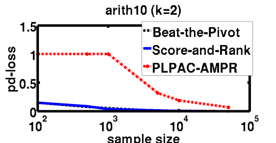
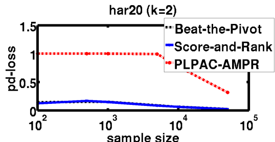
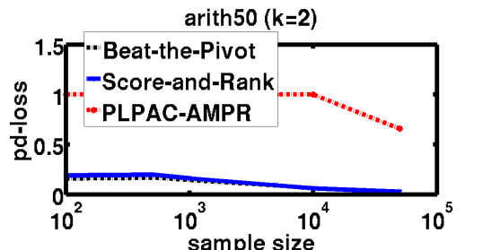
Figure 1: Ranking performance vs. sample size (# rounds) with dueling plays ($k=2$)

Ranking with Pairwise-Preferences ($k=2$). We first compare the above three algorithms with pairwise preference feedback, i.e. with $k=2$ and $m=1$ (WI feedback model). We set $\epsilon=0.01$ and $\delta=0.1$. Figure 1 clearly shows superiority of our two proposed algorithms over PLPAC-AMPR Szörényi et al. (2015) as they give much higher ranking accuracy given the sample size, rightfully justifying our improved theoretical guarantees as well (Theorem 8 and 9). Note that geo8 and arith50 are the easiest and hardest PL model instances, respectively; the latter has the largest $n$ with gaps $\theta_{i}-\theta_{i+1}=0.02$. This also reflects in our experimental results as the ranking estimation loss being the highest for arith50 for all the algorithms, specifically PLPAC-AMPR very poorly till $10^{4}$ samples.

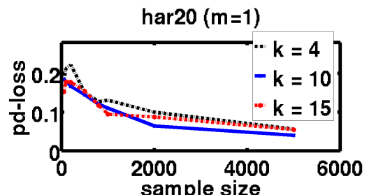
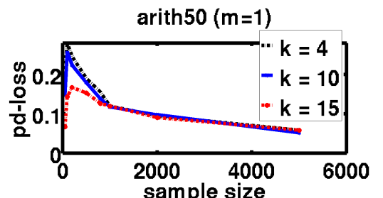
Figure 2: Ranking performance vs. subset size ($k$) with WI feedback ($m=1$)

Ranking with Subsetwise-Preferences ($k>2$ (with winner information (WI) feedback). We next move to the setup of general subsetwise preference feedback $(k\geq 2)$ for WI feedback model (i.e. for $m=1$) . We fix $\epsilon=0.01$ and $\delta=0.1$ and report the performance of Beat-the-Pivot  on the datasets har20 and arith50, varying $k$ over the range $4$ - $40$. As expected from Theorem 8 and explained in Remark 3, the ranking performance indeed does not seem to be varying with increasing subsetsize $k$ for WI feedback model for both PL models (Figure 2).

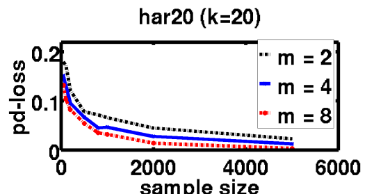
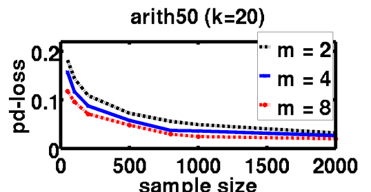
Figure 3: Ranking performance vs. feedback size ($m$) for fixed subset size ($k$)

Ranking with Subsetwise-Preferences ($k>2$ (with top-$m$ ranking (TR) feedback). Lastly we report the performance of Beat-the-Pivot  for top-$m$ ranking (TR) feedback model (Algorithm 5) on two PL models: har20 (for $k=20$) and arith50 (for $k=45$), varying the range of $m$ from $2$ to $40$ (Figure 3). We set $\epsilon=0.01$ and $\delta=0.1$ as before. As expected, in this case it indeed reflects that the the ranking accuracy improves for larger $m$ given a fixed sample size—this reflects over theoretical guarantee of $\frac{1}{m}$-factor improvement of the sample complexity guarantee for TR feedback model (see Theorem 15 and Remark 5).

9 Conclusion and Future Work

We have considered the PAC version of the problem of adaptively ranking $n$ items from $k$-subset-wise comparisons, in the Plackett-Luce (PL) preference model with winner information (WI) and top ranking (TR) feedback. With just WI, the required sample complexity lower bound is $\Omega\Big{(}\frac{n}{\epsilon^{2}}\ln\frac{n}{\delta}\Big{)}$, which is surprisingly independent of the subset size $k$. We have also designed two algorithms enjoying optimal sample complexity guarantees, and based on a novel pivoting-trick. With TR feedback, a $\frac{1}{m}$-times faster learning rate is achievable, and we have given an algorithm with optimal sample complexity guarantees.

In the future, it would be of interest to analyse the problem with other choice models (e.g. multinomial probit, Mallows, nested logit, generalized extreme-value models, etc.), and perhaps to extend this theory to newer formulations such as assortment selection Berbeglia and Joret (2016); Désir et al. (2016), revenue maximization with item prices Talluri and Van Ryzin (2004); Agrawal et al. (2016), or even in contextual scenarios Dudík et al. (2015) where every individual user comes with their own model parameter.

Supplementary for Active Ranking with Subset-wise Preferences

Appendix A Appendix for Section 2

A.1 Proof of Lemma 4

See 4

Recall that an algorithm is defined to be $(\epsilon,\delta)$-PAC-Rank  (or $(\epsilon,\delta)$-PAC-Rank2 ) if it returns an $\epsilon$-Best-Ranking  ($\epsilon$-Best-Ranking-Multiplicative  ) with probability $(1-\delta)$.

Proof.

Case 1. Suppose the algorithm is $(\epsilon,\delta)$-PAC-Rank. So if $\boldsymbol{\sigma}$ is the ranking returned by it, with high probability $(1-\delta)$, $\nexists$ two items $i,j\in[n]$ such that $\sigma(i)>\sigma(j)$ but $\theta_{i}-\theta_{j}\geq\epsilon$. But then this implies, $\nexists$ two items $i,j\in[n]$ with $\sigma(i)>\sigma(j)$ such that

$$Pr(i|\{i,j\})-\frac{1}{2}=\frac{\theta_{i}-\theta_{j}}{2(\theta_{i}-\theta_{j})}\geq\frac{\theta_{i}-\theta_{j}}{4b}=\frac{\epsilon}{4b}\geq\epsilon^{\prime},$$

which proves our first claim.

Case 2. Now suppose the algorithm is $(\epsilon,\delta)$-PAC-Rank-Multiplicative. So if $\boldsymbol{\sigma}$ is the ranking returned by it, with high probability $(1-\delta)$, $\nexists$ two items $i,j\in[n]$ such that $\sigma(i)>\sigma(j)$ but $Pr(i|\{i,j\})-\frac{1}{2}\geq\epsilon$. But since $Pr(i|\{i,j\})=\frac{\theta_{i}}{\theta_{i}+\theta_{j}}$, this them equivalently implies, $\nexists$ two items $i,j\in[n]$ with $\sigma(i)>\sigma(j)$ such that

$$\frac{\theta_{i}}{\theta_{j}}\geq\frac{1/2+\epsilon}{1/2-\epsilon}$$

$$\implies\theta_{i}\geq\theta_{j}\Bigg{(}\frac{1/2+\epsilon}{1/2-\epsilon}\Bigg{)}\geq\theta_{j}\Big{(}{\frac{1}{2}+\epsilon}\Big{)}^{2}$$

$$\implies\theta_{i}-\theta_{j}\geq\theta_{j}\big{(}4\epsilon^{2}+4\epsilon\big{)}\geq 4a\epsilon(1+\epsilon)\geq\epsilon^{\prime},$$

which proves our second claim and concludes the proof.

∎

A.2 Proof of Lemma 5

See 5

Proof.

We prove the lemma by using a coupling argument. Consider the following ‘simulator’ or probability space for the Plackett-Luce choice model that specifically depends on the item pair $i,j$, constructed as follows. Let $Z_{1},Z_{2},\ldots$ be a sequence of iid Bernoulli random variables with success parameter $\theta_{i}/(\theta_{i}+\theta_{j})$. A counter is first initialized to $0$. At each time $t$, given $S_{1},i_{1},\ldots,S_{t-1},i_{t-1}$ and $S_{t}$, an independent coin is tossed with probability of heads $(\theta_{i}+\theta_{j})/\sum_{k\in S_{t}}\theta_{k}$. If the coin lands tails, then $i_{t}$ is drawn as an independent sample from the Plackett-Luce distribution over $S_{t}\setminus\{i,j\}$, else, the counter is incremented by $1$, and $i_{t}$ is returned as $i$ if $Z(C)=1$ or $j$ if $Z(C)=0$ where $C$ is the present value of the counter.

It may be checked that the construction above indeed yields the correct joint distribution for the sequence $i_{1},S_{1},\ldots,i_{T},S_{T}$ as desired, due to the independence of irrelevant alternatives (IIA) property of the Plackett-Luce choice model:

$$Pr(i_{t}=i|i_{t}\in\{i,j\},S_{t})=\frac{Pr(i_{t}=i|S_{t})}{Pr(i_{t}\in\{i,j\}|S_{t})}=\frac{\theta_{i}/\sum_{k\in S_{t}}\theta_{k}}{(\theta_{i}+\theta_{j})/\sum_{k\in S_{t}}\theta_{k}}=\frac{\theta_{i}}{\theta_{i}+\theta_{j}}.$$

Furthermore, $i_{t}\in\{i,j\}$ if and only if $C$ is incremented at round $t$, and $i_{t}=i$ if and only if $C$ is incremented at round $t$ and $Z(C)=1$. We thus have

$$Pr \left(\frac{n_{i}(T)}{n_{ij}(T)}-\frac{\theta_{i}}{\theta_{i}+\theta_{j}}\geq\eta,\;n_{ij}(T)\geq v\right)=Pr\left(\frac{\sum_{\ell=1}^{n_{ij}(T)}Z_{\ell}}{n_{ij}(T)}-\frac{\theta_{i}}{\theta_{i}+\theta_{j}}\geq\eta,\;n_{ij}(T)\geq v\right)$$

$$=\sum_{m=v}^{T}Pr\left(\frac{\sum_{\ell=1}^{n_{ij}(T)}Z_{\ell}}{n_{ij}(T)}-\frac{\theta_{i}}{\theta_{i}+\theta_{j}}\geq\eta,\;n_{ij}(T)=m\right)$$

$$=\sum_{m=v}^{T}Pr\left(\frac{\sum_{\ell=1}^{m}Z_{\ell}}{m}-\frac{\theta_{i}}{\theta_{i}+\theta_{j}}\geq\eta,\;n_{ij}(T)=m\right)$$

$$\stackrel{{\scriptstyle(a)}}{{=}}\sum_{m=v}^{T}Pr\left(\frac{\sum_{\ell=1}^{m}Z_{\ell}}{m}-\frac{\theta_{i}}{\theta_{i}+\theta_{j}}\geq\eta\right)\,Pr\left(n_{ij}(T)=m\right)$$

$$\stackrel{{\scriptstyle(b)}}{{\leq}}\sum_{m=v}^{T}Pr\left(n_{ij}(T)=m\right)\,e^{-2m\eta^{2}}\leq e^{-2v\eta^{2}},$$

where $(a)$ uses the fact that $S_{1},\dots,S_{T},X_{1},\ldots,X_{T}$ are independent of $Z_{1},Z_{2},\ldots,$, and so $n_{ij}(T)\in\sigma(S_{1},\dots,S_{T},X_{1},\ldots,X_{T})$ is independent of $Z_{1},\ldots,Z_{m}$ for any fixed $m$, and $(b)$ uses Hoeffding’s concentration inequality for the iid sequence $Z_{i}$.

Similarly, one can also derive

$$Pr\left(\frac{n_{i}(T)}{n_{ij}(T)}-\frac{\theta_{i}}{\theta_{i}+\theta_{j}}\leq-\eta,\;n_{ij}(T)\geq v\right)\leq e^{-2v\eta^{2}},$$

which concludes the proof. ∎

Appendix B Appendix for Section 4

B.1 Proof of Lemma 6

See 6

Proof.

$(1)$ follows from the simple observation probability of item $b$ winning at any trial $t$ is independent and identically distributed (iid) $Ber\Big{(}\frac{\theta_{b}}{\sum_{j\in S}}\Big{)}$ and $T$ essentially denotes the number of trials till first success (win of $b$). (Recall from Section 2 that $Geo(p)$ denote the ‘number of trials before success’ version of the Geometric random variable with probability of success at each trial being $p\in[0,1]$).

We proof $(2)$ by deriving the moment generating function (MGF) of the random variable $w_{i}(T)$ which gives:

Lemma 18 (MGF of $w_{i}(T)$).

For any item $i\in S\setminus\{b\}$, the moment generating function of the random variable $w_{i}(T)$ is given by: ${\mathbf{E}}\Big{[}e^{\lambda w_{i}(T)}\Big{]}=\frac{1}{1-\frac{\theta_{i}}{\theta_{b}}(e^{\lambda-1})},\forall\ell\in[w_{1}],\,\text{ for any }\lambda\in\big{(}0,\ln(1+\eta)\big{)},\text{ with }\eta<\min_{j\in S}\frac{\theta_{b}}{\theta_{j}}$.

See Appendix B.2 for the proof. Now firstly recall that the MGF of any random variable $X\sim Geo(p)$ is given by ${\mathbf{E}}[e^{\lambda X}]=\frac{p}{(1-e^{\lambda}(1-p))},\,\forall\lambda\in\Big{(}0,-\ln(1-p)\Big{)}$. In the current case $p=\frac{\theta_{b}}{\theta_{b}+\theta_{i}}$. Thus we have $\Bigg{(}\frac{1}{p}-1\Bigg{)}=\frac{\theta_{i}}{\theta_{b}}$ or $\frac{1}{1-p}=\frac{\theta_{i}+\theta_{b}}{\theta_{i}}$, and the MGF holds good for any $\lambda\in(0,\ln(1+\eta))$ as long as $\eta<\min_{j\in S}\frac{\theta_{b}}{\theta_{j}}$.

The proof now follows from straightforward reduction of Lemma 18. Formally, we have:

$${\mathbf{E}}\Big{[}e^{\lambda X}\Big{]} =\frac{p}{(1-e^{\lambda}(1-p))}~{}~{}\text{ for any }\lambda\in\big{(}0,\ln(1+\eta)\big{)},\text{ where }\eta<\min_{j\in S}\frac{\theta_{b}}{\theta_{j}},$$

$$=\frac{1}{\frac{1}{p}-e^{\lambda}\Big{(}\frac{1-p}{p}\Big{)}}=\frac{1}{1+\frac{\theta_{i}}{\theta_{b}}-e^{\lambda}\big{(}\frac{\theta_{i}}{\theta_{b}}\big{)}}$$

$$=\frac{1}{1-\frac{\theta_{i}}{\theta_{b}}(e^{\lambda-1})}={\mathbf{E}}\Big{[}e^{\lambda w_{i}(T)}\Big{]},$$

where the last equality follows from Lemma 18 as two random variables with same MGF must have same distributions. This concludes the proof. ∎

B.2 Proof of Lemma 18

See 18

Proof.

The proof follows from using standard MGF results of Bernoulli and Geometric random variables. We denote $S_{-b}=S{\setminus}\{b\}$, $\hat{T}=(T-1)$, $p=\frac{\theta_{b}}{\sum_{j\in S}\theta_{j}}$, and $p^{\prime}=\frac{\theta_{i}}{\sum_{j\in S_{-b}}\theta_{j}}$. As argued in Lemma 6, we know that ${\hat{T}}\sim$ Geo$\Big{(}p\Big{)}$. Also given a fixed (non-random) ${\hat{T}}$, $w_{i}(T)\sim$ Bin$\Big{(}{\hat{T}},p^{\prime}\Big{)}$. Then using law of iterated expectation:

$${\mathbf{E}}\Big{[}e^{\lambda w_{i}(T)}\Big{]} ={\mathbf{E}}_{{\hat{T}}}\Big{[}{\mathbf{E}}\big{[}e^{\lambda w_{i}(T)}\mid{\hat{T}}\big{]}\Big{]}$$

$$={\mathbf{E}}_{{\hat{T}}}\Big{[}(p^{\prime}e^{\lambda}+1-p^{\prime})^{{\hat{T}}}\Big{]},$$

where the last equality follows from the MGF of Binomial random variables. Note that, since $\lambda>0$, we have $(p^{\prime}e^{\lambda}+1-p^{\prime})=1+p^{\prime}(e^{\lambda}-1)>1$. Let us denote $\lambda^{\prime}=\ln(1+p^{\prime}(e^{\lambda}-1))$. Clearly $\lambda^{\prime}>0$ as both $\lambda,p^{\prime}>0$. Then from above equation, one can write:

$${\mathbf{E}}\Big{[}e^{\lambda w_{i}(T)}\Big{]} ={\mathbf{E}}_{{\hat{T}}}\Big{[}e^{\lambda^{\prime}{\hat{T}}}\Big{]},$$

$$=\frac{p}{(1-e^{\lambda^{\prime}}(1-p))}$$

$$=\frac{p}{1-(1+p^{\prime}(e^{\lambda}-1))(1-p)}=\frac{1}{1-\frac{\theta_{i}}{\theta_{b}}(e^{\lambda-1})},$$

where the second equality follows from the result that MGF of a geometric random variable $X\sim$ Geo$(p)$ is: ${\mathbf{E}}[e^{\lambda^{\prime}X}]=\frac{p}{(1-e^{\lambda^{\prime}}(1-p))},\,\forall\lambda^{\prime}\in\Big{(}0,-\ln(1-p)\Big{)}$.

Thus the only remaining thing to show is $\lambda^{\prime}$ indeed satisfies the above range. As argues above, clearly $\lambda^{\prime}>0$ as both $\lambda,p^{\prime}>0$. To verify the upper bound, note that by choice $\lambda<\ln\Big{(}1+\frac{\theta_{b}}{\theta_{j}}\Big{)},\,\forall j\in S$, which implies $e^{\lambda}<(1+\frac{\theta_{b}}{\theta_{i}})$, for any $i\in S_{-b}$. This further implies $(e^{\lambda}-1)\frac{\theta_{i}}{\theta_{b}}<1\implies(1-\frac{\theta_{i}}{\theta_{b}}(e^{\lambda}-1))>0\implies(1-p)(1+p^{\prime}(e^{\lambda}-1))<1$ rearranging which leads to the desired bound $\lambda^{\prime}<-\ln(1-p)$ (recall $\lambda^{\prime}=\ln(1+p^{\prime}(e^{\lambda}-1))$, and thus the above MGF holds good. This concludes the proof. ∎

B.3 Proof of Lemma 7

See 7

Proof.

The result follows from the concentration of Geometric random variable as shown in Brown [2011]. Note that, $Z$ denotes the number of trials needed to get $n$ wins of item $b$, where the probability of success (i.e. item $b$ winning) at each trial is $\frac{\theta_{b}}{\theta_{b}+\theta_{i}}$. Thus $Z\sim$ NB$(n,\frac{\theta_{b}}{\theta_{b}+\theta_{i}})$. Clearly, by applying union bounding we get:

$$Pr\Big{(}\Big{|}\frac{Z}{n}-\frac{\theta_{i}}{\theta_{b}}\Big{|}>\eta\Big{)}\leq Pr\Big{(}\frac{Z}{n}-\frac{\theta_{i}}{\theta_{b}}>\eta\Big{)}+Pr\Big{(}\frac{Z}{n}-\frac{\theta_{i}}{\theta_{b}}<-\eta\Big{)}.$$

Let us start by analysing the first term $Pr\Big{(}\frac{Z}{n}-\frac{\theta_{i}}{\theta_{b}}>\eta\Big{)}$.

$$Pr \Big{(}\frac{Z}{n}-\frac{\theta_{i}}{\theta_{b}}>\eta\Big{)}=Pr\Big{(}Z>n\frac{\theta_{i}}{\theta_{b}}+n\eta\Big{)}$$

$$\leq Pr\Bigg{(}Bin\bigg{(}n(\frac{\theta_{i}}{\theta_{b}}+1)+n\eta,\frac{\theta_{b}}{\theta_{b}+\theta_{i}}\bigg{)}<n\Bigg{)}$$

$$\leq Pr\Bigg{(}Bin\bigg{(}n(\frac{\theta_{i}}{\theta_{b}}+1)+n\eta,\frac{\theta_{b}}{\theta_{b}+\theta_{i}}\bigg{)}-\bigg{[}n(\frac{\theta_{i}}{\theta_{b}}+1)+n\eta\bigg{]}\frac{1}{1+\frac{\theta_{i}}{\theta_{b}}}<-\frac{n\eta}{1+\frac{\theta_{i}}{\theta_{b}}}\Bigg{)}$$

$$\leq\exp\Big{(}-\frac{2}{m}\tilde{\eta}^{2}\Big{)}=\exp\Bigg{(}-\frac{2n\eta^{2}}{\Big{(}1+\frac{\theta_{i}}{\theta_{b}}\Big{)}^{2}\Big{(}\eta+1+\frac{\theta_{i}}{\theta_{b}}\Big{)}}\Bigg{)}$$ (1)

where the last inequality follows simply apply Hoeffding’s inequality with $m=n(\frac{\theta_{i}}{\theta_{b}}+1)+n\eta$ and $\tilde{\eta}=\frac{n\eta}{1+\frac{\theta_{i}}{\theta_{b}}}$. Using a similar derivation as before, one can also show:

$$Pr\Big{(}\frac{Z}{n}-\frac{\theta_{i}}{\theta_{b}}<-\eta\Big{)}\leq\exp\Bigg{(}-\frac{2n\eta^{2}}{\Big{(}1+\frac{\theta_{i}}{\theta_{b}}\Big{)}^{2}\Big{(}\eta+1+\frac{\theta_{i}}{\theta_{b}}\Big{)}}\Bigg{)}$$ (2)

The result now follows combining (B.3) and (2). ∎

Appendix C Appendix for Section 5

C.1 Proof of Lemma 10

See 10

Proof.

We start by analyzing the required sample complexity first. Note that the ‘while loop’ of Algorithm 3 always discards away $k-1$ items per iteration. Thus, $n$ being the total number of items the loop can be executed is at most for $\lceil\frac{n}{k-1}\rceil$ many number of iterations. Clearly, the sample complexity of each iteration being $t=\frac{2k}{\epsilon^{2}}\ln\frac{2\delta}{n}$, the total sample complexity of the algorithm becomes $\big{(}\lceil\frac{n}{k-1}\rceil\big{)}\frac{2k}{\epsilon^{2}}\ln\frac{n}{2\delta}\leq\big{(}\frac{n}{k-1}+1\big{)}\frac{2k}{\epsilon^{2}}\ln\frac{n}{2\delta}=\big{(}n+\frac{n}{k-1}+k\big{)}\frac{2}{\epsilon^{2}}\ln\frac{n}{2\delta}=O(\frac{n}{\epsilon^{2}}\ln\frac{n}{\delta})$.

We now prove the $(\epsilon,\delta)$-PAC correctness of the algorithm. As argued before, the ‘while loop’ of Algorithm 3 can run for maximum $\lceil\frac{n}{k-1}\rceil$ many number of iterations. We denote the iterations by $\ell=1,2,\ldots\lceil\frac{n}{k-1}\rceil$, and the corresponding set ${\mathcal{A}}$ of iteration $\ell$ by ${\mathcal{A}}_{\ell}$.

Note that our idea is to retain the estimated best item in ‘running winner’ $r_{\ell}$ and compare it with the ‘empirical best item’ $c_{\ell}$ of ${\mathcal{A}}_{\ell}$ at every iteration $\ell$. The crucial observation lies in noting that at any iteration $\ell$, $r_{\ell}$ gets updated as follows:

Lemma 19.

At any iteration $\ell=1,2\ldots\big{\lfloor}\frac{n}{k-1}\big{\rfloor}$, with probability at least $(1-\frac{\delta}{2n})$, Algorithm 3 retains $r_{\ell+1}\leftarrow r_{\ell}$ if $p_{c_{\ell}r_{\ell}}\leq\frac{1}{2}$, and sets $r_{\ell+1}\leftarrow c_{\ell}$ if $p_{c_{\ell}r_{\ell}}\geq\frac{1}{2}+\epsilon$.

Proof.

Consider any set ${\mathcal{A}}_{\ell}$, by which we mean the state of ${\mathcal{A}}$ in the algorithm at iteration $\ell$. The crucial observation to make is that since $c_{\ell}$ is the empirical winner of $t$ rounds, then $w_{c_{\ell}}\geq\frac{t}{k}$. Thus $w_{c_{\ell}}+w_{r_{\ell}}\geq\frac{t}{k}$. Let $n_{ij}:=w_{i}+w_{j}$ denotes the total number of pairwise comparisons between item $i$ and $j$ in $t$ rounds, for any $i,j\in{\mathcal{A}}_{\ell}$. Then clearly, $0\leq n_{ij}\leq t$ and $n_{ij}=n_{ji}$. Specifically we have ${\hat{p}}_{r_{\ell}c_{\ell}}=\frac{w_{r_{\ell}}}{w_{r_{\ell}}+w_{c_{\ell}}}=\frac{w_{r_{\ell}}}{n_{r_{\ell}c_{\ell}}}$. We prove the claim by analyzing the following cases:

Case 1. (If $p_{c_{\ell}r_{\ell}}\leq\frac{1}{2}$, Find-the-Pivot  retains $r_{\ell+1}\leftarrow r_{\ell}$): Note that Find-the-Pivot  replaces $r_{\ell+1}$ by $c_{\ell}$ only if ${\hat{p}}_{c_{\ell},r_{\ell}}>\frac{1}{2}+\frac{\epsilon}{2}$, but this happens with probability:

$$Pr\Bigg{(}\bigg{\{}{\hat{p}}_{c_{\ell}r_{\ell}}>\frac{1}{2}+\frac{\epsilon}{2}\bigg{\}}\Bigg{)}$$

$$=Pr\Bigg{(}\bigg{\{}{\hat{p}}_{c_{\ell}r_{\ell}}>\frac{1}{2}+\frac{\epsilon}{2}\bigg{\}}\cap\bigg{\{}n_{c_{\ell}r_{\ell}}\geq\frac{t}{k}\bigg{\}}\Bigg{)}+\cancelto{0}{Pr\bigg{\{}n_{c_{\ell}r_{\ell}}<\frac{t}{k}\bigg{\}}}Pr\Bigg{(}\bigg{\{}{\hat{p}}_{c_{\ell}r_{\ell}}>\frac{1}{2}+\frac{\epsilon}{2}\bigg{\}}\Big{|}\bigg{\{}n_{c_{\ell}r_{\ell}}<\frac{t}{k}\bigg{\}}\Bigg{)}$$

$$\leq Pr\Bigg{(}\bigg{\{}{\hat{p}}_{c_{\ell}r_{\ell}}-p_{c_{\ell}r_{\ell}}>\frac{\epsilon}{2}\bigg{\}}\cap\bigg{\{}n_{c_{\ell}r_{\ell}}\geq\frac{t}{k}\bigg{\}}\Bigg{)}\leq\exp\Big{(}-2\dfrac{t}{k}\bigg{(}\frac{\epsilon}{2}\bigg{)}^{2}\Big{)}=\frac{\delta}{2n},$$

where the first inequality follows as $p_{c_{\ell}r_{\ell}}\leq\frac{1}{2}$, and the second inequality is by applying Lemma 5 with $\eta=\frac{\epsilon}{2}$ and $v=\frac{t}{k}$. We now proceed to the second case:

Case 2. (If $p_{c_{\ell}r_{\ell}}\geq\frac{1}{2}+\epsilon$, Find-the-Pivot  sets $r_{\ell+1}\leftarrow c_{\ell}$): Recall again that Find-the-Pivot  retains $r_{\ell+1}\leftarrow r_{\ell}$ only if ${\hat{p}}_{c_{\ell},r_{\ell}}\leq\frac{1}{2}+\frac{\epsilon}{2}$. This happens with probability:

$$Pr\Bigg{(}\bigg{\{}{\hat{p}}_{c_{\ell}r_{\ell}}\leq\frac{1}{2}+\frac{\epsilon}{2}\bigg{\}}\Bigg{)}$$

$$=Pr\Bigg{(}\bigg{\{}{\hat{p}}_{c_{\ell}r_{\ell}}\leq\frac{1}{2}+\frac{\epsilon}{2}\bigg{\}}\cap\bigg{\{}n_{c_{\ell}r_{\ell}}\geq\frac{t}{k}\bigg{\}}\Bigg{)}+\cancelto{0}{Pr\bigg{\{}n_{c_{\ell}r_{\ell}}<\frac{t}{k}\bigg{\}}}Pr\Bigg{(}\bigg{\{}{\hat{p}}_{c_{\ell}r_{\ell}}\leq\frac{1}{2}+\frac{\epsilon}{2}\bigg{\}}\Big{|}\bigg{\{}n_{c_{\ell}r_{\ell}}<\frac{t}{k}\bigg{\}}\Bigg{)}$$

$$=Pr\Bigg{(}\bigg{\{}{\hat{p}}_{c_{\ell}r_{\ell}}\leq\frac{1}{2}+\epsilon-\frac{\epsilon}{2}\bigg{\}}\cap\bigg{\{}n_{c_{\ell}r_{\ell}}\geq\frac{t}{k}\bigg{\}}\Bigg{)}$$

$$\leq Pr\Bigg{(}\bigg{\{}{\hat{p}}_{c_{\ell}r_{\ell}}-p_{c_{\ell}r_{\ell}}\leq-\frac{\epsilon}{2}\bigg{\}}\cap\bigg{\{}n_{c_{\ell}r_{\ell}}\geq\frac{t}{k}\bigg{\}}\Bigg{)}\leq\exp\Big{(}-2\dfrac{t}{k}\bigg{(}\frac{\epsilon}{2}\bigg{)}^{2}\Big{)}=\frac{\delta}{2n},$$

where the first inequality holds as $p_{c_{\ell}r_{\ell}}\geq\frac{1}{2}+\epsilon$, and the second one by applying Lemma 5 with $\eta=\frac{\epsilon}{2}$ and $v=\frac{t}{k}$. Combining the above two cases concludes the proof. ∎

Given Algorithm 3 satisfies Lemma 19, and taking union bound over $(k-1)$ elements in ${\mathcal{A}}_{\ell}\setminus\{r_{\ell}\}$, we get that with probability at least $(1-\frac{(k-1)\delta}{2n})$,

$$p_{r_{\ell+1}r_{\ell}}\geq\frac{1}{2}\text{ and, }p_{r_{\ell+1}c_{\ell}}\geq\frac{1}{2}-\epsilon.$$ (3)

Above suggests that for each iteration $\ell$, the estimated ‘best’ item $r_{\ell}$ only gets improved as $p_{r_{\ell+1}r_{\ell}}\geq\frac{1}{2}$. Let, $\ell_{*}$ denotes the specific iteration such that $1\in{\mathcal{A}}_{\ell}$ for the first time, i.e. $\ell_{*}=\min\{\ell\mid 1\in{\mathcal{A}}_{\ell}\}$. Clearly $\ell_{*}\leq\lceil\frac{n}{k-1}\rceil$. Now (3) suggests that with probability at least $(1-\frac{(k-1)\delta}{2n})$, $p_{r_{\ell_{*}+1}1}\geq\frac{1}{2}-\epsilon$. Moreover (3) also suggests that for all $\ell>\ell_{*}$, with probability at least $(1-\frac{(k-1)\delta}{2n})$, $p_{r_{\ell+1}r_{\ell}}\geq\frac{1}{2}$, which implies for all $\ell>\ell_{*}$, $p_{r_{\ell+1}1}\geq\frac{1}{2}-\epsilon$ as well – This holds due to the following transitivity property of the Plackett-Luce model: For any three items $i_{1},i_{2},i_{3}\in[n]$, if $p_{i_{1}i_{2}}\geq\frac{1}{2}$ and $p_{i_{2}i_{3}}\geq\frac{1}{2}$, then we have $p_{i_{1}i_{3}}\geq\frac{1}{2}$ as well.

This argument finally leads to $p_{r_{*}1}\geq\frac{1}{2}-\epsilon$. Since failure probability at each iteration $\ell$ is at most $\frac{(k-1)\delta}{2n}$, and Algorithm 3 runs for maximum $\lceil\frac{n}{k-1}\rceil$ many number of iterations, using union bound over $\ell$, the total failure probability of the algorithm is at most $\lceil\frac{n}{k-1}\rceil\frac{(k-1)\delta}{2n}\leq(\frac{n}{k-1}+1)\frac{(k-1)\delta}{2n}=\delta\Big{(}\frac{n+k-1}{2n}\Big{)}\leq\delta$ (since $k\leq n$). This concludes the correctness of the algorithm showing that it indeed satisfies the $(\epsilon,\delta)$-PAC objective.∎

C.2 Proof of Theorem 8

See 8

Proof.

We first analyze the sample complexity of Beat-the-Pivot. Clearly, there are at most $G=\lceil\frac{n-1}{k-1}\rceil\leq\frac{n-1}{k-1}+1\leq\frac{2(n-1)}{k-1}$ groups. Here the last inequality follows since $n\geq k$. Now each group ${\mathcal{G}}_{g}$ (set of $k$ items) is played (queried) for at most $t:=\frac{2k}{\epsilon^{\prime 2}}\log\frac{1}{\delta^{\prime}}$ times, which gives the total sample complexity of the algorithm to be

$$G*t\leq\frac{2(n-1)}{(k-1)}*\frac{2k}{\epsilon^{\prime 2}}\log\frac{1}{\delta^{\prime}}=\frac{2048(n-1)}{\epsilon^{2}}\log\frac{8n}{\delta}=O\Big{(}\frac{n}{\epsilon^{2}}\log\frac{n}{\delta}\Big{)},$$

where we used the fact $k\geq 2$ and bound $\frac{k}{k-1}\leq 2$.

Moreover the sample complexity of Find-the-Pivot  is also $O\Big{(}\frac{n}{\epsilon^{2}}\log\frac{n}{\delta}\Big{)}$ as proved in Lemma 10. Combining this with above thus makes the total sample complexity of Beat-the-Pivot  $O\Big{(}\frac{n}{\epsilon^{2}}\log\frac{n}{\delta}\Big{)}$.

We are now only left to show the correctness of the algorithm, i.e. Beat-the-Pivot  indeed $(\epsilon,\delta)$-PAC-Rank  in the above sample complexity. We start by proving the following lemma which would be crucial throughout the analysis. Let us first denote $\Delta^{b}_{ij}=P(i\succ b)-P(j\succ b),\,$ for any $i$ and $j\in[n]$.

Lemma 20.

If $b$ is the pivot-item returned by Algorithm 3 (Line $5$ of Beat-the-Pivot), then for any two items $i,j\in[n]$, such that $\theta_{i}\geq\theta_{j}$, $\frac{(\theta_{i}-\theta_{j})}{8}\leq\Delta^{b}_{ij}\leq 4(\theta_{i}-\theta_{j})$, with probability at least $\big{(}1-\frac{\delta}{2}\big{)}$.

Proof.

First let us assume if $b=1$. Then $\Delta^{b}_{ij}=P(i\succ 1)-P(j\succ 1)=\frac{\theta_{1}(\theta_{i}-\theta_{j})}{(\theta_{j}+\theta_{1})(\theta_{i}+\theta_{1})}\geq\frac{(\theta_{i}-\theta_{j})}{4}$, since $\theta_{1}=1$ and $\theta_{i}\leq 1,~{}\forall i\in[n]$. On the other hand, we also have $\Delta^{b}_{ij}=P(i\succ 1)-P(j\succ 1)=\frac{\theta_{1}(\theta_{i}-\theta_{j})}{(\theta_{j}+\theta_{1})(\theta_{i}+\theta_{1})}\leq(\theta_{i}-\theta_{j})={\epsilon}$, since $\theta_{1}=1$ and $\theta_{i}\geq 0,\forall i\in[n]$.

However even if $b\neq 1$, with high probability $(1-\frac{\delta}{2})$, it is ensured that $\theta_{b}>\theta_{1}-\frac{1}{2}$, as with high probability $(1-\frac{\delta}{2})$, Algorithm 3 returns an $\epsilon$-Best-Item (see Lemma 10, proof in Appendix C.1). Then similarly as before, $\Delta^{b}_{ij}=P(i\succ 1)-P(j\succ 1)=\frac{\theta_{b}(\theta_{i}-\theta_{j})}{(\theta_{j}+\theta_{b})(\theta_{i}+\theta_{b})}\geq\frac{(\theta_{i}-\theta_{j})}{8}$, $\theta_{b}\geq\theta_{1}-\frac{1}{2}=\frac{1}{2}$, and $\theta_{i}\leq 1,~{}\forall i\in[n]$. On the other hand, we also have $\Delta^{b}_{ij}=P(i\succ b)-P(j\succ b)=\frac{\theta_{b}(\theta_{i}-\theta_{j})}{(\theta_{j}+\theta_{b})(\theta_{i}+\theta_{b})}\leq 4(\theta_{i}-\theta_{j})={\epsilon}$, since $\theta_{b}\in\big{(}\frac{1}{2},1]$, and $\theta_{i}\geq 0,~{}\forall i\in[n]$. This proves our claim. ∎

Now to ensure the correctness of Beat-the-Pivot, recall that all we need to show it returns an $\epsilon$-Best-Ranking $\boldsymbol{\sigma}\in\Sigma_{[n]}$. The main idea is to plug in the pivot item $b$ in every group ${\mathcal{G}}_{g}$ and estimate the pivot-preference score $p_{ib}=Pr(i\succ b)$ of every item $i\notin{\mathcal{G}}_{g}\setminus\{b\}$, i.e. with respect to the pivot item $b$. We finally output the ranking simply sorting the items w.r.t. $p_{ib}$ – the intuition is if item $i$ beats $j$ in terms of their actual BTL scores (i.e. $\theta_{i}>\theta_{j}$), then $i$ beats $j$ in terms of their pivot-preference scores as well (i.e. $p_{ib}>p_{jb}$).

More formally, as $\boldsymbol{\sigma}$ denotes the ranking returned by Beat-the-Pivot, the algorithm fails if $\boldsymbol{\sigma}$ is not $\epsilon$-Best-Ranking. We denote by $Pr_{b}(\cdot)=Pr(\cdot\big{|}b\text{ is }\epsilon_{b}\text{-\emph{Best-Item}})$ the probability of an event conditioned on the event that $b$ is indeed an $\epsilon_{b}$-Best-Item (Recall we have set $\epsilon_{b}=\min(\frac{\epsilon}{2},\frac{1}{2})$). Formally, we have:

$$Pr_{b}(\text{ {\it Beat-the-Pivot}\, fails }) =Pr_{b}(\exists i,j\in[n]\mid\theta_{i}>\theta_{j}+\epsilon\text{ but }\sigma(i)>\sigma(j))$$ (4)

$$=Pr_{b}(\exists i,j\in[n]\mid\theta_{i}>\theta_{j}+\epsilon\text{ but }{\hat{p}}_{ib}<{\hat{p}}_{jb})$$

Now, assuming $b$ to be indeed an $\epsilon_{b}$-Best-Item, since $\theta_{i}>\theta_{j}\implies\Delta_{ij}^{b}\geq\frac{\epsilon}{8}$ (from Lemma 20), from Eqn. 4, we further get:

$$Pr_{b}(\text{ {\it Beat-the-Pivot}\, fails }) =Pr_{b}(\exists i,j\in[n]\mid\theta_{i}>\theta_{j}+\epsilon\text{ but }\sigma(i)>\sigma(j))$$

$$\leq Pr_{b}\Big{(}\exists i,j\in[n]\setminus\{b\}\mid p_{ib}>p_{jb}+\frac{\epsilon}{8}\text{ but }\sigma(i)>\sigma(j)\Big{)}$$

$$=Pr_{b}(\exists i,j\in[n]\setminus\{b\}\mid\Delta_{ij}^{b}>\frac{\epsilon}{8}\text{ but }{\hat{p}}_{ib}<{\hat{p}}_{jb}),$$ (5)

where the inequality follows due to Lemma 20. In the inequality of the above analysis, it is also crucial to note that under the assumption of $b$ to be indeed an $\epsilon_{b}$-Best-Item setting $\sigma(1)=b$ does not incur an error since $\theta_{b}>\theta_{1}-\frac{\epsilon}{2}$. So if we can estimate each $p_{ib}$ within a confidence interval of $\frac{\epsilon}{16}$, that should be enough to ensure correctness of the algorithm. Thus the only thing remaining to show is Beat-the-Pivot  indeed estimates $p_{ib}$ tightly enough with high confidence – formally, it is enough to show that for any group $g\in[G]$ and any item $i\in{\mathcal{G}}_{g}\setminus\{b\}$, $Pr_{b}\Big{(}|p_{ib}-{\hat{p}}_{ib}|>\frac{\epsilon}{16}\Big{)}\leq\frac{\delta}{4n}$.

We prove this using the following two lemmas. We first show that in any set ${\mathcal{G}}_{g}$, if it is played for $m$ times, then with high probability of at least $(1-\delta)$, the pivot item would gets selected at least for $\frac{m}{4k}$ times. Formally:

Lemma 21.

Conditioned on the event that $b$ is indeed an $\epsilon_{b}$-Best-Item, for any group $g\in[G]$ with probability at least $\Big{(}1-\dfrac{\delta}{8n}\Big{)}$, the empirical win count $w_{b}>(1-\eta)\frac{t}{2k}$, for any $\eta\in\big{(}\frac{1}{8\sqrt{2}},1\big{]}$.

Proof.

We will assume the event that $b$ to be indeed an $\epsilon_{b}$-Best-Item throughout the proof and use the shorthand notation $Pr_{b}(\cdot)$ as defined earlier. The proof now follows from an straightforward application of Chernoff-Hoeffding’s inequality Boucheron et al. [2013]. Recall that the algorithm plays each set ${\mathcal{G}}_{g}$ for $t=\frac{2k}{\epsilon^{\prime 2}}\ln\frac{1}{\delta^{\prime}}$ number of times. Now consider a fixed group $g\in[G]$ and let $i_{\tau}$ denotes the winner of the $\tau$-th play of ${\mathcal{G}}_{g}$, $\tau\in[t]$. Clearly, for any item $i\in{\mathcal{G}}_{g}$, $w_{i}=\sum_{\tau=1}^{t}{\mathbf{1}}(i_{\tau}==i)$, where ${\mathbf{1}}(i_{\tau}==i)$ is a Bernoulli random variable with parameter $\frac{\theta_{i}}{\sum_{j\in{\mathcal{G}}_{g}}\theta_{j}}$, $\forall\tau\in[t]$, just by the definition of the PL query model with winner information (WI) (Sec. 3.1). Thus the random variable $w_{i}\sim Bin\Big{(}t,\frac{\theta_{i}}{\sum_{j\in{\mathcal{G}}_{g}}\theta_{j}}\Big{)}$. In particular, for the pivot item, $i=b$, we have $Pr_{b}(\{i_{\tau}=b\})=\frac{\theta_{b}}{\sum_{j\in{\mathcal{G}}_{g}}\theta_{j}}\geq\dfrac{\frac{1}{2}}{k}$. Hence ${\mathbf{E}}[w_{b}]=\sum_{\tau=1}^{t}{\mathbf{E}}[{\mathbf{1}}(i_{\tau}==b)]\geq\frac{t}{2k}$. Now applying multiplicative Chernoff-Hoeffdings bound for $w_{b}$, we get that for any $\eta\in\Big{(}\frac{1}{8},1\Big{]}$,

$$Pr_{b}\Big{(}w_{b}\leq(1-\eta){\mathbf{E}}[w_{b}]\Big{)} \leq\exp\Big{(}-\frac{{\mathbf{E}}[w_{b}]\eta^{2}}{2}\Big{)}\leq\exp\Big{(}-\frac{t\eta^{2}}{4k}\Big{)},~{}\Big{(}\text{since }{\mathbf{E}}[w_{b}]\geq\frac{t}{2k}\Big{)}$$

$$\leq\exp\bigg{(}-\frac{\eta^{2}}{2\epsilon^{\prime 2}}\ln\bigg{(}\frac{1}{\delta^{\prime}}\bigg{)}\bigg{)}\leq\exp\bigg{(}-\ln\bigg{(}\frac{1}{\delta^{\prime}}\bigg{)}\bigg{)}\leq\frac{\delta}{8n},$$

where the second last inequality holds for any $\eta>\frac{1}{8\sqrt{2}}$ as it has to be the case that $\epsilon^{\prime}<\frac{1}{16}$ since $\epsilon\in(0,1)$. Thus for any $\eta>\frac{1}{8\sqrt{2}}$, $\eta^{2}\geq 4\epsilon^{\prime 2}$. ∎

In particular, choosing $\eta=\frac{1}{2}$ in Lemma 21, we have with probability at least $\Big{(}1-\dfrac{\delta}{8n}\Big{)}$, the empirical win count of the pivot element $b$ is at least $w_{b}>\frac{t}{4k}$. We next proof under $w_{b}>\frac{t}{4k}$, the estimate of pivot-preference scores $p_{ib}$ can not be too bad for any item $i\in{\mathcal{G}}_{g}$ at any group $g\in[G]$. The formal statement is given in Lemma 22. For the ease of notation we define the event ${\mathcal{E}}_{g}:=\{\exists i\in{\mathcal{G}}_{g}\setminus\{b\}\text{ s.t. }|p_{ib}-{\hat{p}}_{ib}|>\frac{\epsilon}{16}\}$.

Lemma 22.

Conditioned on the event that $b$ is indeed an $\epsilon_{b}$-Best-Item, for any group $g\in[G]$, $Pr_{b}\Big{(}{\mathcal{E}}_{g}\Big{)}\leq\frac{k\delta}{4n}$.

Proof.

We will again assume the event that $b$ to be indeed an $\epsilon_{b}$-Best-Item throughout the proof and use the shorthand notation $Pr_{b}(\cdot)$ as defined previously. Let us first fix a group $g\in[G]$. We find convenient to define the event ${\mathcal{F}}_{g}=\{w_{b}\geq\frac{t}{4k}\text{ for group }{\mathcal{G}}_{g}\}$ and denote by $n^{g}_{ib}=w_{i}+w_{b}$ the total number of times item $i$ and $b$ has won in group ${\mathcal{G}}_{g}$. Clearly, $n^{g}_{ib}\leq t$, moreover under ${\mathcal{F}}_{g}$, $n^{g}_{ib}\geq\frac{t}{4k},\,\forall i\in{\mathcal{G}}_{g}$. Then for any item $i\in{\mathcal{G}}_{g}\setminus\{b\}$,

$$Pr_{b}\Bigg{(}\bigg{\{}|p_{ib}-{\hat{p}}_{ib}|>\frac{\epsilon}{16}\bigg{\}}\cap{\mathcal{F}}_{g}\Bigg{)} \leq Pr_{b}\Bigg{(}\bigg{\{}|p_{ib}-{\hat{p}}_{ib}|>\frac{\epsilon}{16}\bigg{\}}\cap\bigg{\{}n^{g}_{ib}\geq\frac{t}{4k}\bigg{\}}\Bigg{)}$$

$$\leq 2\exp\Big{(}-2\frac{t}{4k}\big{(}\frac{\epsilon}{16}\big{)}^{2}\Big{)}=\frac{\delta}{4n},$$ (6)

where the first inequality follows since ${\mathcal{F}}_{g}\implies n^{g}_{ib}\geq\frac{t}{4k}$, the second inequality holds due to Lemma 5 with $\eta=\frac{\epsilon}{16}$, and $v=\frac{t}{4k}$. Its crucial to note that while applying 5, we can so we can drop the notation $Pr_{b}(\cdot)$ as the event $\{|p_{ib}-{\hat{p}}_{ib}|>\frac{\epsilon}{16}\}\cap\bigg{\{}n^{g}_{ib}\geq\frac{t}{4k}\bigg{\}}$ is independent of $b$ to be $\epsilon_{b}$-Best-Item or not.

Then probability that Beat-the-Pivot  fails to estimate the pivot-preference scores $p_{ib}$ for group ${\mathcal{G}}_{g}$,

$$Pr_{b}({\mathcal{E}}_{g}) =Pr_{b}({\mathcal{E}}_{g}\cap{\mathcal{F}}_{g})+Pr_{b}({\mathcal{E}}_{g}\cap{\mathcal{F}}_{g}^{c})$$

$$\leq Pr_{b}({\mathcal{E}}_{g}\cap{\mathcal{F}}_{g})+Pr_{b}({\mathcal{F}}_{g}^{c})$$

$$\leq Pr_{b}({\mathcal{E}}_{g}\cap{\mathcal{F}}_{g})+\frac{\delta}{8n}~{}~{}\Big{(}\text{From Lemma \ref{lem:ant_pivpickup}}\Big{)}$$

$$\leq\sum_{i\in{\mathcal{G}}_{g}\setminus\{b\}}Pr_{b}\Bigg{(}\bigg{\{}|p_{ib}-{\hat{p}}_{ib}|>\frac{\epsilon}{16}\bigg{\}}\cap{\mathcal{F}}_{g}\Bigg{)}+\frac{\delta}{8n}$$

$$=(k-1)\frac{\delta}{4n}+\frac{\delta}{4n}\leq\frac{k\delta}{4n},$$

where the last inequality follows by taking union bound. The last equality follows from (C.2) and hence the proof follows. ∎

Thus using Lemma 22 and from (C.2) we get,

$$Pr_{b}( \text{{\it Beat-the-Pivot}\, fails })\leq Pr_{b}(\exists i,j\in[n]\setminus\{b\}\mid\Delta_{ij}^{b}>\frac{\epsilon}{8}\text{ but }{\hat{p}}_{ib}<{\hat{p}}_{jb})$$

$$\leq Pr_{b}(\exists g\in[G]\text{ s.t. }{\mathcal{E}}_{g})=\Big{(}\bigg{\lceil}\frac{n-1}{k-1}\bigg{\rceil}\Big{)}\frac{k\delta}{4n}\leq 2\Big{(}\frac{n-1}{k-1}\Big{)}\frac{k\delta}{4n}\leq\frac{\delta}{2},$$ (7)

where the last inequality follows taking union bound over all groups $g\in[G]$. Finally analysing all the previous claims together:

$$Pr(\text{{\it Beat-the-Pivot}\, fails })$$

$$\leq Pr(\text{{\it Beat-the-Pivot}\, fails }\big{|}b\text{ is an }\epsilon_{b}\text{-\emph{Best-Item}})Pr(b\text{ is an }\epsilon_{b}\text{-\emph{Best-Item}})+Pr(b\text{ is not an }\epsilon_{b}\text{-\emph{Best-Item}})$$

$$\leq Pr_{b}(\text{{\it Beat-the-Pivot}\, fails })\Big{(}1-\frac{\delta}{2}\Big{)}+\frac{\delta}{2}\leq\frac{\delta}{2}+\frac{\delta}{2}=\delta,$$

where the last inequality follows from (C.2), which concludes the proof. ∎

C.3 Proof of Theorem 9

See 9

Proof.

Before proving the sample complexity, we first show the correctness of the algorithm, i.e. Beat-the-Pivot  is indeed $(\epsilon,\delta)$-PAC-Rank. The following lemma would be crucially used throughout the proof analysis. Let us first denote $\theta_{i}^{b}=\frac{\theta_{i}}{\theta_{b}}$ the score of item $i\in[n]$ with respect to that of item $b$, we will term it as pivotal-score of item $i$. Also let $\theta^{b}_{ij}=\theta_{i}^{b}-\theta_{j}^{b},\,$ for any $i$ and $j\in[n]$. It is easy to note that since with high probability $(1-\frac{\delta}{4})$, $\frac{1}{2}\leq\theta_{b}\leq 1$ (Lemma 10), and hence $\theta_{i}\leq\theta_{i}^{b}\leq 2\theta_{i}$. This further leads to the following claim:

Lemma 23.

If $b$ is the pivot-item returned by Algorithm 3 (Line $5$ of Score-and-Rank), then for any two items $i,j\in[n]$, such that $\theta_{i}\geq\theta_{j}$, $(\theta_{i}-\theta_{j})\leq\theta^{b}_{ij}\leq 2(\theta_{i}-\theta_{j})$, with probability at least $\big{(}1-\frac{\delta}{4}\big{)}$.

Proof.

First let us assume if $b=1$, which implies $\theta_{i}^{b}=\frac{\theta_{i}}{\theta_{b}}=\theta_{i}$ and the claims holds trivially.

Now let us assume that $b\neq 1$, but by Lemma 10, with high probability, $\theta_{b}\geq\theta_{1}-\frac{1}{2}=\frac{1}{2}$ as Find-the-Pivot  returns an $\epsilon_{b}$-Best-Item with probability at least $(1-\frac{\delta}{4})$. Also $\theta_{b}\leq 1$ for any $b\neq 1$. The above bounds on $\theta_{b}$ clearly implies $\theta^{b}_{ij}=\frac{\theta_{i}-\theta_{j}}{\theta_{b}}\in\Big{[}(\theta_{i}-\theta_{j}),2(\theta_{i}-\theta_{j})\Big{]}$. ∎

Now to ensure the correctness of Beat-the-Pivot, recall that all we need to show it returns an $\epsilon$-Best-Ranking $\boldsymbol{\sigma}\in\Sigma_{[n]}$. Same as Algorithm 1, here also we plug in the pivot item $b$ in every group ${\mathcal{G}}_{g}$. But now it estimates the pivotal score $\theta_{i}^{b}$ of every item $i\notin{\mathcal{G}}_{g}\setminus\{b\}$ instead of pivotal preference score $p_{ib}$ where lies the uniqeness of Score-and-Rank. We finally output the ranking simply sorting the items w.r.t. $\theta_{i}^{b}$ – the intuition is if item $i$ beats $j$ in terms of their actual BTL scores (i.e. $\theta_{i}>\theta_{j}$), then $i$ beats $j$ in terms of their pivotal scores as well (i.e. $\theta_{i}^{b}>\theta_{j}^{b}$).

More formally, as $\boldsymbol{\sigma}$ denotes the ranking returned by Beat-the-Pivot, the correctness of algorithm Score-and-Rank  fails if $\boldsymbol{\sigma}$ is not an $\epsilon$-Best-Ranking. Formally, we have:

$$Pr(\text{ Correctness of {\it Beat-the-Pivot}\, fails }) =Pr(\exists i,j\in[n]\mid\theta_{i}>\theta_{j}+\epsilon\text{ but }\sigma(i)>\sigma(j))$$ (8)

$$=Pr(\exists i,j\in[n]\mid\theta_{i}>\theta_{j}+\epsilon\text{ but }{\hat{\theta}}_{i}^{b}<{\hat{\theta}}_{j}^{b})$$

Now, assuming $b$ to be indeed an $\epsilon_{b}$-Best-Item, since $\theta_{i}>\theta_{j}\implies\theta_{ij}^{b}\geq\epsilon$ (from Lemma 23), from Eqn. 8, we further get:

$$Pr(\text{ Correctness of {\it Beat-the-Pivot}\, fails }) =Pr(\exists i,j\in[n]\mid\theta_{i}>\theta_{j}+\epsilon\text{ but }\sigma(i)>\sigma(j))$$

$$\leq Pr\Big{(}\exists i,j\in[n]\setminus\{b\}\mid\theta_{i}^{b}>\theta_{j}^{b}+\epsilon\text{ but }\sigma(i)>\sigma(j)\Big{)}$$

$$=Pr(\exists i,j\in[n]\setminus\{b\}\mid\theta_{i}^{b}>\theta_{j}^{b}+\epsilon\text{ but }{\hat{\theta}}_{i}^{b}<{\hat{\theta}}_{j}^{b}),$$ (9)

where the inequality follows due to Lemma 23. In the inequality of the above analysis, it is also crucial to note that under the assumption of $b$ to be indeed an $\epsilon_{b}$-Best-Item setting $\sigma(1)=b$ does not incur an error since $\theta_{b}>\theta_{1}-\frac{\epsilon}{2}$. So if we can estimate each ${\hat{\theta}}_{i}^{b}$ within a confidence interval of $\frac{\epsilon}{2}$, that should be enough to ensure correctness of the algorithm. Thus the only thing remaining to show is Score-and-Rank  indeed estimates $\theta_{i}^{b}$ tightly enough with high confidence – formally, it is enough to show that for any group $g\in[G]$ and any item $i\in{\mathcal{G}}_{g}\setminus\{b\}$, $Pr\Big{(}|\theta_{i}^{b}-{\hat{\theta}}_{i}^{b}|>\frac{\epsilon}{2}\Big{)}\leq\frac{\delta}{4n}$.

For this we will be crucially using the result of Lemma 6, which shows that ${\hat{\theta}}_{i}^{b}\sim Geo\Big{(}\dfrac{\theta_{b}}{\theta_{i}+\theta_{b}}\Big{)}$ for any item $i\in{\mathcal{G}}_{g}$ and at any group $g\in[G]$.

Using the above insight, we will show that the estimate of pivotal scores ${\hat{\theta}}_{i}^{b}$ can not be too bad for any item $i\in{\mathcal{G}}_{g}$ at any group $g\in[G]$. The formal statement is given in Lemma 22. For the ease of notation let us define the event ${\mathcal{E}}_{g}:=\{\exists i\in{\mathcal{G}}_{g}\setminus\{b\}\text{ s.t. }|\theta_{i}^{b}-{\hat{\theta}}_{i}^{b}|>\frac{\epsilon}{2}\}$.

Lemma 24.

For any group $g\in[G]$, $Pr\Big{(}{\mathcal{E}}_{g}\Big{)}\leq\frac{(k-1)\delta}{4n}$.

Proof.

We will again assume the event that $b$ to be indeed an $\epsilon_{b}$-Best-Item throughout the proof and use the shorthand notation $Pr_{b}(\cdot)$ as defined previously. Let us first fix a group $g\in[G]$. Then for any item $i\in{\mathcal{G}}_{g}\setminus\{b\}$,

$$Pr\Big{(}|{\hat{\theta}}_{i}^{b}-\theta_{i}^{b}|>\frac{\epsilon}{2}\Big{)}\leq 2\exp\Bigg{(}-\frac{2t(\epsilon/2)^{2}}{\Big{(}1+\frac{\theta_{i}}{\theta_{b}}\Big{)}^{2}\Big{(}(\epsilon/2)+1+\frac{\theta_{i}}{\theta_{b}}\Big{)}}\Bigg{)}=\frac{\delta}{4n},$$ (10)

where the inequality follows from Lemma 7. Then summing over, all the items $i\in{\mathcal{G}}_{g}{\setminus}\{b\}$ in group $g\in[G]$,

$$Pr_{b}({\mathcal{E}}_{g}) \leq\sum_{i\in{\mathcal{G}}_{g}\setminus\{b\}}Pr\Bigg{(}|{\hat{\theta}}_{i}^{b}-\theta_{i}^{b}|>\frac{\epsilon}{2}\Bigg{)}=(k-1)\frac{\delta}{4n},$$

where the inequality follows from (10). ∎

Now applying Lemma 24 over all groups $g\in[G]$, and using (C.3), the probability that correctness of Score-and-Rank  fails:

$$Pr( \text{ Correctness of {\it Beat-the-Pivot}\, fails })\leq Pr(\exists i,j\in[n]\setminus\{b\}\mid\theta_{i}^{b}>\theta_{j}^{b}+\epsilon\text{ but }{\hat{\theta}}_{i}^{b}<{\hat{\theta}}_{j}^{b})$$

$$\leq Pr_{b}(\exists g\in[G]\text{ s.t. }{\mathcal{E}}_{g})=\Big{(}\bigg{\lceil}\frac{n-1}{k-1}\bigg{\rceil}\Big{)}\frac{(k-1)\delta}{4n}\leq 2\Big{(}\frac{n-1}{k-1}\Big{)}\frac{(k-1)\delta}{4n}\leq\frac{\delta}{2},$$ (11)

where the last inequality follows taking union bound over all groups $g\in[G]$.

Thus we are now only left to prove that the correctness of Score-and-Rank  indeed holds within the desired sample complexity of $O\big{(}\frac{n}{\epsilon^{2}}\log\frac{n}{\delta}\big{)}$. Towards this, let us first define $t^{\prime}=\frac{5}{2}tk=\frac{5*567k}{2\epsilon^{2}}\ln\big{(}\frac{8n}{\delta}\big{)}$. Also let $Pr_{b}(\cdot)=Pr(\cdot\big{|}b\text{ is }\epsilon_{b}\text{-\emph{Best-Item}})$ denotes the probability of an event conditioned on the event that $b$ is indeed an $\epsilon_{b}$-Best-Item (Recall we have set $\epsilon_{b}=\min(\frac{\epsilon}{2},\frac{1}{2})$). For any group $g\in[G]$, we denote by ${\mathcal{T}}_{g}$ the total number of times ${\mathcal{G}}_{g}$ was played until $t$ wins of item $b$ were observed. Also recall the probability of item $b$ being the winner at any subsetwise play of ${\mathcal{C}}_{g}$ is given by $p:=\frac{\theta_{b}}{\sum_{j\in{\mathcal{G}}_{g}}\theta_{j}}>\frac{1}{2k}$, given $b$ is indeed an $\epsilon_{b}$-Best-Item (from Lemma 10). So we have the ${\mathcal{T}}_{g}\sim$ NB$(t,\frac{\theta_{b}}{\sum_{j\in{\mathcal{G}}_{g}}\theta_{j}})$. Then for any fixed group $g\in[G]$, the probability that ${\mathcal{G}}_{g}$ needs to be played (queried) for more than $t^{\prime}$ times to get at least $t$ wins of item $b$:

$$Pr_{b}({\mathcal{T}}_{g}>t^{\prime}) =Pr\Big{(}Bin(t^{\prime},p)<t\Big{)}$$

$$\leq Pr\Big{(}Bin(t^{\prime},p)<\frac{4}{5}pt^{\prime}\Big{)}~{}~{}\Bigg{[}\text{ Since }pt^{\prime}>\frac{5tk}{4k}\Bigg{]}$$

$$=Pr\Big{(}Bin(t^{\prime},p)-pt^{\prime}<-\frac{1}{5}pt^{\prime}\Big{)}$$

$$\leq Pr\Big{(}Bin(t^{\prime},p)-pt^{\prime}<(1-\frac{4}{5})pt^{\prime}\Big{)}$$

$$\leq\exp\Big{(}-\frac{pt^{\prime}(4/5)^{2}}{2}\Big{)}~{}~{}\Bigg{[}\text{ By multiplicative Chernoff bound }\Bigg{]}$$

$$\leq\exp\Big{(}-\frac{2}{5}t\Big{)}~{}~{}\Bigg{[}\text{ Using }pt^{\prime}>\frac{5t}{4}\Bigg{]}$$

$$\leq\frac{\delta}{8n}~{}~{}\Bigg{[}\text{ Recall we have }t=\frac{567}{4\big{(}\epsilon/2\big{)}^{2}}\ln\big{(}\frac{8n}{\delta}\big{)}\Bigg{]}$$

Then taking union bound over all the groups

$$Pr(\exists g\in[G]\mid{\mathcal{T}}_{g}>t^{\prime}) \leq Pr_{b}(\exists g\in[G]\mid{\mathcal{T}}_{g}>t^{\prime})Pr(\theta_{b}>\theta_{1}-\epsilon_{b})+Pr(\theta_{b}<\theta_{1}-\epsilon_{b})$$

$$\leq Pr_{b}(\exists g\in[G]\mid{\mathcal{T}}_{g}>t^{\prime})+\frac{\delta}{4}\leq\sum_{g\in[G]}Pr_{b}({\mathcal{T}}_{g}>t^{\prime})+\frac{\delta}{4}$$

$$\leq\Big{(}\lceil\frac{n-1}{k-1}\rceil\Big{)}\frac{\delta}{8n}+\frac{\delta}{4}\leq 2\Big{(}\frac{n-1}{k-1}\Big{)}\frac{\delta}{8n}+\frac{\delta}{4}\leq\frac{\delta}{2}.$$ (12)

Then with high probability $(1-\frac{\delta}{2})$, $\forall g\in[G]$ we have ${\mathcal{T}}_{g}<t^{\prime}=\frac{5}{2}tk$, which makes the total sample complexity of Score-and-Rank  to be at most $\Big{\lceil}\frac{n-1}{k-1}\Big{\rceil}t^{\prime}\leq\frac{2n}{k}\frac{5tk}{2}=\frac{2835n}{\epsilon^{2}}\ln\frac{8n}{\delta}=O\bigg{(}\frac{n}{\epsilon^{2}}\ln\frac{n}{\delta}\bigg{)}$, as total number of groups are $G=\lceil\frac{n-1}{k-1}\rceil$.

Moreover the sample complexity of Find-the-Pivot  is also $O\Big{(}\frac{n}{\epsilon^{2}}\log\frac{n}{\delta}\Big{)}$ as proved in Lemma 10. Combining this with above the total sample complexity of Beat-the-Pivot  remains $O\Big{(}\frac{n}{\epsilon^{2}}\log\frac{n}{\delta}\Big{)}$. Finally analysing all the previous claims together:

$$Pr(\text{{\it Beat-the-Pivot}\, fails })$$

$$\leq Pr(\text{ Correctness of {\it Beat-the-Pivot}\, fails })+Pr(\text{ Sample complexity of {\it Beat-the-Pivot}\, fails })$$

$$\leq\frac{\delta}{2}+\frac{\delta}{2}=\delta,$$

where the last inequality follows from (C.3) and (C.3), which concludes the proof. ∎

Appendix D Appendix for Section 6

D.1 Restating Lemma 1 of Kaufmann et al. [2016]

Consider a multi-armed bandit (MAB) problem with $n$ arms. At round $t$, let $A_{t}$ and $Z_{t}$ denote the arm played and the observation (reward) received, respectively. Let ${\mathcal{F}}_{t}=\sigma(A_{1},Z_{1},\ldots,A_{t},Z_{t})$ be the sigma algebra generated by the trajectory of a sequential bandit algorithm upto round $t$.

Lemma 25 (Lemma $1$, Kaufmann et al. [2016]).

Let $\nu$ and $\nu^{\prime}$ be two bandit models (assignments of reward distributions to arms), such that $\nu_{i}~{}(\text{resp.}\,\nu^{\prime}_{i})$ is the reward distribution of any arm $i\in{\mathcal{A}}$ under bandit model $\nu~{}(\text{resp.}\,\nu^{\prime})$, and such that for all such arms $i$, $\nu_{i}$ and $\nu^{\prime}_{i}$ are mutually absolutely continuous. Then for any almost-surely finite stopping time $\tau$ with respect to $({\mathcal{F}}_{t})_{t}$,

$$\sum_{i=1}^{n}{\mathbf{E}}_{\nu}[N_{i}(\tau)]KL(\nu_{i},\nu_{i}^{\prime})\geq\sup_{{\mathcal{E}}\in{\mathcal{F}}_{\tau}}kl(Pr_{\nu}({\mathcal{E}}),Pr_{\nu^{\prime}}({\mathcal{E}})),$$

where $kl(x,y):=x\log(\frac{x}{y})+(1-x)\log(\frac{1-x}{1-y})$ is the binary relative entropy, $N_{i}(\tau)$ denotes the number of times arm $i$ is played in $\tau$ rounds, and $Pr_{\nu}({\mathcal{E}})$ and $Pr_{\nu^{\prime}}({\mathcal{E}})$ denote the probability of any event ${\mathcal{E}}\in{\mathcal{F}}_{\tau}$ under bandit models $\nu$ and $\nu^{\prime}$, respectively.

D.2 Proof of Lemma 13

See 13

Proof.

Base Case. The claim follows trivially for $q=1$, just from the definition of $(\epsilon,\delta)$-PAC-Rank property of the algorithm. Suppose $S=\{i\}$ for some $i\in[n-1]$. Then clearly

$$Pr_{S}\Big{(}\boldsymbol{\sigma}_{{\mathcal{A}}}(1)=\{0\}\Big{)}<Pr_{S}\Big{(}\boldsymbol{\sigma}_{{\mathcal{A}}}(1)\neq\{i\}\Big{)}<\delta.$$

So for the rest of the proof we focus only on the regime where $2\leq q\leq n-1$. Let us first fix an $q^{\prime}\in[n-2]$ and set $q=q^{\prime}+1$. Clearly $2\leq q\leq n-1$. Consider a problem instance $\nu_{S}\in{\boldsymbol{\nu}}_{[q]}$. Recall from Remark 1 that we use the notation $S\in{\boldsymbol{\nu}}_{[q]}$ to denote a problem instance in ${\boldsymbol{\nu}}_{[q]}$. Then probability of doing an error over all possible choices of $S\in{\boldsymbol{\nu}}_{[q]}$:

$$\sum_{S\in{\boldsymbol{\nu}}_{[q]}}Pr_{S}\Big{(}\boldsymbol{\sigma}_{{\mathcal{A}}}(1:q)\neq S\Big{)} \geq\sum_{S\in{\boldsymbol{\nu}}_{[q^{\prime}+1]}}\sum_{i\in S}Pr_{S}\Big{(}\boldsymbol{\sigma}_{{\mathcal{A}}}(1:q)=S{\setminus}\{i\}\cup\{0\}\Big{)}$$

$$=\sum_{S^{\prime}\in{\boldsymbol{\nu}}_{[q^{\prime}]}}\sum_{i\in[n-1]\setminus S^{\prime}}Pr_{S^{\prime}\cup\{i\}}\Big{(}\boldsymbol{\sigma}_{{\mathcal{A}}}(1:q)=S^{\prime}\cup\{0\}\Big{)},$$ (13)

where the above analysis follows from a similar result proved by Kalyanakrishnan et al. [2012] to derive sample complexity lower bound for classical multi-armed bandit setting towards recovering top-$q$ items (see Theorem $8$, Kalyanakrishnan et al. [2012]).

Clearly the possible number of instances in ${\boldsymbol{\nu}}_{[q^{\prime}]}$, i.e. $|{\boldsymbol{\nu}}_{[q^{\prime}]}|={{n-1}\choose{q^{\prime}}}$, as any set $S\subset[n-1]$ of size $q^{\prime}$ can be chosen from $[n-1]$ in ${{n-1}\choose{q^{\prime}}}$ ways. Similarly, $|{\boldsymbol{\nu}}_{[q]}|={{n-1}\choose{q}}={{n-1}\choose{q^{\prime}+1}}$.

Now from symmetry of algorithm ${\mathcal{A}}$ and by construction of the class of our problem instances ${\boldsymbol{\nu}}_{[q^{\prime}]}$, for any two instances $S^{\prime}_{1}$ and $S^{\prime}_{2}$ in ${\boldsymbol{\nu}}_{[q^{\prime}]}$, and for any choices of $i\in[n-1]\setminus S^{\prime}_{1}$ and $j\in[n-1]\setminus S^{\prime}_{2}$ we have that:

$$Pr_{S^{\prime}_{1}\cup\{i\}}\Big{(}\boldsymbol{\sigma}_{{\mathcal{A}}}(1:q)=S^{\prime}_{1}\cup\{0\}\Big{)}=Pr_{S^{\prime}_{2}\cup\{j\}}\Big{(}\boldsymbol{\sigma}_{{\mathcal{A}}}(1:q)=S^{\prime}_{2}\cup\{0\}\Big{)}.$$

Let us denote $Pr_{S^{\prime}_{1}\cup\{i\}}\Big{(}\boldsymbol{\sigma}_{{\mathcal{A}}}=\boldsymbol{\sigma}_{S^{\prime}_{1}}\Big{)}=p^{\prime}\in(0,1)$. Then above equivalently implies that for all $S\in{\boldsymbol{\nu}}_{[q]}$ and any $i\in[n-1]\setminus S$,

$$Pr_{S}(\boldsymbol{\sigma}_{{\mathcal{A}}}(1:q)=S\setminus\{i\}\cup\{0\})=p^{\prime}.$$

Then using above in (D.2) we can further derive,

$$\sum_{S\in{\boldsymbol{\nu}}_{[q]}}Pr_{S}\Big{(}\boldsymbol{\sigma}_{{\mathcal{A}}}(1:q)\neq{S}\Big{)} \geq\sum_{S^{\prime}\in{\boldsymbol{\nu}}_{[q^{\prime}]}}\sum_{i\in[n-1]\setminus S^{\prime}}Pr_{S^{\prime}\cup\{i\}}\Big{(}\boldsymbol{\sigma}_{{\mathcal{A}}}(1:q)=S^{\prime}\cup\{0\}\Big{)}$$

$$=\sum_{S^{\prime}\in{\boldsymbol{\nu}}_{[q^{\prime}]}}(n-1-q^{\prime})p^{\prime}$$

$$={{n-1}\choose{q^{\prime}}}(n-1-q^{\prime})p^{\prime}$$

$$={{n-1}\choose{q^{\prime}}}\frac{n-1-q^{\prime}}{q^{\prime}+1}(q+1)p^{\prime}$$

$$={{n-1}\choose{q^{\prime}+1}}(q^{\prime}+1)p^{\prime}={{n-1}\choose{q}}qp^{\prime}.$$

But now observe that $|{\boldsymbol{\nu}}_{[q]}|={{n-1}\choose{q}}$. Thus if $p^{\prime}\geq\frac{\delta}{q}$, this implies

$$\sum_{S\in{\boldsymbol{\nu}}_{[q]}}Pr_{S}\Big{(}\boldsymbol{\sigma}_{{\mathcal{A}}}(1:q)\neq{S}\Big{)}\geq{{n-1}\choose{q}}{\delta},$$

which in turn implies that there exist at least one instance $\nu_{S}\in{\boldsymbol{\nu}}_{[q+1]}$ such that $Pr_{S}\Big{(}\boldsymbol{\sigma}_{{\mathcal{A}}}(1:q)\neq S\Big{)}\geq\delta$, which violates the $(\epsilon,\delta)$-PAC-Rank property of algorithm ${\mathcal{A}}$. Thus it has to be the case that $p^{\prime}<\frac{\delta}{q}$. Recall that we have chosen $2\leq q\leq n-1$, and for any $S\in{\boldsymbol{\nu}}_{[q]}$, and any $i\in[n-1]\setminus S$ we proved that

$$Pr_{S}(\boldsymbol{\sigma}_{{\mathcal{A}}}(1:q)=S\setminus\{i\}\cup\{0\})=p^{\prime}<\frac{\delta}{q},$$

which concludes the proof. ∎

D.3 Proof of Lemma 26

Lemma 26.

For any $\delta\in(0,1)$, and $q\in{\mathbb{R}}_{+}$, $kl\bigg{(}1-\delta,\dfrac{\delta}{q}\bigg{)}>\ln\dfrac{q}{4\delta}.$

Proof.

The proof simply follows from the definition of KL divergence. Recall that for any $p_{1},p_{2}\in(0,1)$,

$$kl(p_{1},p_{2})=p_{1}\ln\frac{p_{1}}{p_{2}}+(1-p_{1})\ln\frac{1-p_{1}}{1-p_{2}}.$$

Applying above in our case we get,

$$kl\bigg{(}1-\delta,\frac{\delta}{q}\bigg{)} =(1-\delta)\ln\frac{q(1-\delta)}{\delta}+\delta\ln\frac{q(\delta)}{(q-\delta)}$$

$$=(1-\delta)\ln\frac{q(1-\delta)}{\delta}+\delta\ln\frac{q(\delta)}{(q-\delta)}$$

$$=\ln q+(1-\delta)\ln\frac{(1-\delta)}{\delta}+\delta\ln\frac{(\delta)}{(q-\delta)}$$

$$\geq\ln q+(1-\delta)\ln\frac{(1-\delta)}{\delta}+\delta\ln\frac{(\delta)}{(1-\delta)}~{}~{}[\text{ since }q\geq 1]$$

$$=\ln q+(1-2\delta)\ln\frac{(1-\delta)}{\delta}$$

$$\geq\ln q+(1-2\delta)\ln\frac{1}{2\delta}~{}~{}\Big{[}\text{ since the second term is negative for }\delta\geq\frac{1}{2}\Big{]}$$

$$=\ln q+\ln\frac{1}{2\delta}+2\delta\ln 2\delta$$

$$\geq\ln q+\ln\frac{1}{2\delta}+2\delta\Big{(}1-\frac{1}{2\delta}\Big{)}~{}~{}\Big{[}\text{ since }x\ln x\geq(x-1),\,\forall x>0\Big{]}$$

$$=\ln q+\ln\frac{1}{2\delta}-(1-2\delta)$$

$$\geq\ln q+\ln\frac{1}{2\delta}+\ln\frac{1}{2}=\ln\frac{q}{4\delta}.$$

∎

D.4 Proof of Theorem 12

See 12

Proof.

The main idea lies in constructing ‘hard enough’ problem instances on which no algorithm can be $(\epsilon,\delta)$-PAC-Rank without observing $\Omega\bigg{(}\frac{n}{\epsilon^{2}}\ln\frac{1}{4\delta}\bigg{)}$ number of samples. We crucially use the results of Kaufmann et al. [2016] (Lemma 25) for the purpose.

Towards this we first fix our true problem instance ($\nu$ in Lemma 25) to be $\nu_{S^{*}}\in{\boldsymbol{\nu}}_{[q]}$, for some $q\in[n-2]$ (the actual value of $q$ to be decided later). Note that the arm set ${\mathcal{B}}$ (of Lemma 25) for our current problem setup is set of all $k$-sized subsets of $[n-1]\cup\{0\}$, i.e. ${\mathcal{B}}=\{S\subseteq[n-1]\cup\{0\}\mid|S|=k\}$.

We now fix the altered problem instance ($\nu^{\prime}$ in Lemma 25) to be $\nu_{{\tilde{S}}^{*}}\in{\boldsymbol{\nu}}_{[q+1]}$ such that ${\tilde{S}}^{*}=S^{*}\cup\{a\}$, of some $a\in[n-1]\setminus S^{*}$. Now if $\boldsymbol{\sigma}_{{\mathcal{A}}}\in\Sigma_{[n]}$ is the ranking returned by Algorithm ${\mathcal{A}}$, then clearly owing to the $(\epsilon,\delta)$-PAC-Rank property of ${\mathcal{A}}$,

$$Pr_{{S^{*}}}\Big{(}\boldsymbol{\sigma}_{{\mathcal{A}}}(1:q+1)=S^{*}\cup\{0\}\Big{)}>Pr_{{S^{*}}}\big{(}\{\boldsymbol{\sigma})_{{\mathcal{A}}}\text{ is an {\it$\epsilon$-Best-Ranking}}\}\big{)}>(1-\delta),$$ (14)

Moreover the $(\epsilon,\delta)$-PAC-Rank property of ${\mathcal{A}}$ also implies that:

$$Pr_{{\tilde{S}}^{*}}\Big{(}\boldsymbol{\sigma}_{{\mathcal{A}}}(1:q+1)=S^{*}\cup\{0\}\Big{)}\leq Pr_{{\tilde{S}}^{*}}\Big{(}\boldsymbol{\sigma}_{{\mathcal{A}}}\neq\boldsymbol{\sigma}_{{\tilde{S}}^{*}}\Big{)}<\delta.$$

But owing to Lemma 13, we are able to claim a stronger bound (using $S={\tilde{S}}^{*}$):

$$Pr_{{\tilde{S}}^{*}}\Big{(}\boldsymbol{\sigma}_{{\mathcal{A}}}(1:q+1)=S^{*}\cup\{0\}\Big{)}<\frac{\delta}{q}.$$ (15)

We will crucially use (14) and (15) in the following analysis. But before that note that for problem instance $\nu_{S^{*}}\in{\boldsymbol{\nu}}_{[q]}$, the probability distribution associated with a particular arm (set of size $k$ in our case) $B\in{\mathcal{B}}$ is given by:

$$\nu^{B}_{S^{*}}\sim Categorical(p_{1},p_{2},\ldots,p_{k}),\text{ where }p_{i}=Pr(i|B),~{}~{}\forall i\in[k],\,\forall B\in{\mathcal{B}},$$

where $Pr(i|S)$ is as defined in Sec. (3.1). Now applying Lemma 25, for some event ${\mathcal{E}}\in{\mathcal{F}}_{\tau}$ we get,

$$\sum_{\{B\in{\mathcal{B}}:a\in B\}}{\mathbf{E}}_{\nu^{B}_{S^{*}}}[N_{B}(\tau_{{\mathcal{A}}})]KL(\nu^{B}_{S^{*}},\nu^{B}_{{\tilde{S}}^{*}})\geq{kl(Pr_{\nu^{B}_{S^{*}}}({\mathcal{E}}),Pr_{\nu^{B}_{{\tilde{S}}^{*}}}({\mathcal{E}}))},$$ (16)

where $N_{B}(\tau_{{\mathcal{A}}})$ denotes the number of times arm (subset of size $k$) $B$ is played by ${\mathcal{A}}$ in $\tau$ rounds. Above clearly follows due to the fact that for any arm $B\in{\mathcal{B}}$ such that $a\notin B$, $\nu^{B}_{S}$ is same as $\nu^{B}_{{\tilde{S}}^{*}}$, and hence $KL(\nu^{B}_{S^{*}},\nu^{B}_{{\tilde{S}}^{*}})=0$, $\forall S\in{\mathcal{A}},\,a\notin S$. For the notational convenience we will henceforth denote ${\mathcal{B}}^{a}=\{B\in{\mathcal{B}}:a\in S\}$.

Now let us first analyse the right hand side of (16), for any set $B\in{\mathcal{B}}^{a}$.

Case 1. Assume $0\notin B$, and denote by $r=|B\cap{S^{*}}|$ the number of “good” arms with PL parameter $\theta\Big{(}\frac{1}{2}+\epsilon\Big{)}^{2}$. Note that for problem instance $\nu_{{S^{*}}}^{B}$,

$$\nu^{B}_{{S^{*}}}(i)=\begin{cases}\frac{\theta(\frac{1}{2}+\epsilon)^{2}}{r\theta(\frac{1}{2}+\epsilon)^{2}+(k-r)\theta(\frac{1}{2}-\epsilon)^{2}}=\frac{R^{2}}{rR^{2}+(k-r)},\forall i\in[k],\text{ such that }B(i)\in S^{*},\\ \frac{\theta(\frac{1}{2}-\epsilon)^{2}}{r\theta(\frac{1}{2}+\epsilon)^{2}+(k-r)\theta(\frac{1}{2}-\epsilon)^{2}}=\frac{1}{rR^{2}+(k-r)},\text{ otherwise. }\end{cases}$$

Similarly, for problem instance $\nu_{{\tilde{S}}^{*}}^{B}$, we have:

$$\nu^{B}_{{\tilde{S}}^{*}}(i)=\begin{cases}\frac{\theta(\frac{1}{2}+\epsilon)^{2}}{(r+1)\theta(\frac{1}{2}+\epsilon)^{2}+(k-r-1)\theta(\frac{1}{2}-\epsilon)^{2}}=\frac{R^{2}}{(r+1)R^{2}+(k-r-1)},\forall i\in[k],\text{ such that }B(i)\in{\tilde{S}}^{*}={S^{*}}\cup\{a\},\\ \frac{\theta(\frac{1}{2}-\epsilon)^{2}}{(r+1)\theta(\frac{1}{2}+\epsilon)^{2}+(k-r-1)\theta(\frac{1}{2}-\epsilon)^{2}}=\frac{1}{(r+1)R^{2}+(k-r-1)},\text{ otherwise. }\end{cases}$$

Now using the following upper bound on $KL({\mathbf{p}}_{1},{\mathbf{p}}_{2})\leq\sum_{x\in{\mathcal{X}}}\frac{p_{1}^{2}(x)}{p_{2}(x)}-1$, ${\mathbf{p}}_{1}$ and ${\mathbf{p}}_{2}$ be two probability mass functions on the discrete random variable ${\mathcal{X}}$ Popescu et al. [2016] we get:

$$KL(\nu^{B}_{S^{*}},\nu^{B}_{{\tilde{S}}^{*}}) \leq\frac{(r+1)R^{2}+(k-r-1)}{(rR^{2}+k-r)^{2}}\Big{[}rR^{2}+\frac{1}{R^{2}}+(k-r-1)\Big{]}-1$$

$$=\Big{(}R-\frac{1}{R}\Big{)}^{2}\Big{[}\frac{rR^{2}+(k-r-1)}{(rR^{2}+k-r)^{2}}\Big{]}$$ (17)

Case 2. Now assume $0\in B$, and denote by $r=|B\cap{S^{*}}\cup\{0\}|$ the number of “non-bad” arms with PL parameter greater than $\theta\Big{(}\frac{1}{2}-\epsilon\Big{)}^{2}$. Clearly $r\geq 1$ as $0\in B$. Similar to Case 1, for problem instance $\nu_{{S^{*}}}^{B}$,

$$\nu^{B}_{{S^{*}}}(i)=\begin{cases}\frac{\theta(\frac{1}{2}+\epsilon)^{2}}{(r-1)\theta(\frac{1}{2}+\epsilon)^{2}+(k-r)\theta(\frac{1}{2}-\epsilon)^{2}+\theta(\frac{1}{4}-\epsilon^{2})}=\frac{R^{2}}{(r-1)R^{2}+(k-r)+R},\forall i\in[k],\text{ such that }B(i)\in S^{*},\\ \frac{\theta(\frac{1}{4}-\epsilon^{2})}{(r-1)\theta(\frac{1}{2}+\epsilon)^{2}+(k-r)\theta(\frac{1}{2}-\epsilon)^{2}+\theta(\frac{1}{4}-\epsilon^{2})}=\frac{R}{(r-1)R^{2}+(k-r)+R},\forall i\in[k],\text{ such that }B(i)=0,\\ \frac{\theta(\frac{1}{2}-\epsilon)^{2}}{(r-1)\theta(\frac{1}{2}+\epsilon)^{2}+(k-r)\theta(\frac{1}{2}-\epsilon)^{2}+\theta(\frac{1}{4}-\epsilon^{2})}=\frac{1}{(r-1)R^{2}+(k-r)+R},\text{ otherwise. }\end{cases}$$

Similarly, for problem instance $\nu_{{\tilde{S}}^{*}}^{B}$, we have:

$$\nu^{B}_{{\tilde{S}}^{*}}(i)=\begin{cases}\frac{\theta(\frac{1}{2}+\epsilon)^{2}}{r\theta(\frac{1}{2}+\epsilon)^{2}+(k-r-1)\theta(\frac{1}{2}-\epsilon)^{2}+\theta(\frac{1}{4}-\epsilon^{2})}=\frac{R^{2}}{rR^{2}+(k-r-1)+R},\forall i\in[k],\text{ such that }B(i)\in{\tilde{S}}^{*}={S^{*}}\cup\{a\},\\ \frac{\theta(\frac{1}{4}-\epsilon^{2})}{r\theta(\frac{1}{2}+\epsilon)^{2}+(k-r-1)\theta(\frac{1}{2}-\epsilon)^{2}+\theta(\frac{1}{4}-\epsilon^{2})}=\frac{R}{rR^{2}+(k-r-1)+R},\forall i\in[k],\text{ such that }B(i)=0,\\ \frac{\theta(\frac{1}{2}-\epsilon)^{2}}{r\theta(\frac{1}{2}+\epsilon)^{2}+(k-r-1)\theta(\frac{1}{2}-\epsilon)^{2}+\theta(\frac{1}{4}-\epsilon^{2})}=\frac{1}{rR^{2}+(k-r-1)+R},\text{ otherwise. }\end{cases}$$

Same as before, again using the following upper bound on $KL({\mathbf{p}}_{1},{\mathbf{p}}_{2})\leq\sum_{x\in{\mathcal{X}}}\frac{p_{1}^{2}(x)}{p_{2}(x)}-1$, ${\mathbf{p}}_{1}$ and ${\mathbf{p}}_{2}$ be two probability mass functions on the discrete random variable ${\mathcal{X}}$ Popescu et al. [2016] we get:

$$KL(\nu^{B}_{S^{*}},\nu^{B}_{{\tilde{S}}^{*}}) \leq\frac{rR^{2}+R+(k-r-1)}{((r-1)R^{2}+R+k-r)^{2}}\Big{[}rR^{2}+\frac{1}{R^{2}}+(k-r-1)\Big{]}-1$$

$$=\Big{(}R-\frac{1}{R}\Big{)}^{2}\Bigg{[}\frac{(r-1)R^{2}+(k-r)+R-1}{\big{(}(r-1)R^{2}+(k-r)+R\big{)}^{2}}\Bigg{]}$$ (18)

Now, consider ${\mathcal{E}}_{0}\in{\mathcal{F}}_{\tau}$ be an event such that ${\mathcal{E}}_{0}:=\{\boldsymbol{\sigma}_{{\mathcal{A}}}(1:q+1)=S^{*}\cup\{0\}\}$. Note that since algorithm ${\mathcal{A}}$ is $(\epsilon,\delta)$-PAC-Rank , clearly $Pr_{\nu^{B}_{S^{*}}}({\mathcal{E}}_{0})>Pr_{\nu^{B}_{S^{*}}}\big{(}\{\boldsymbol{\sigma})_{{\mathcal{A}}}\text{ is an {\it$\epsilon$-Best-Ranking}}\}\big{)}>(1-\delta)$. On the other hand, Lemma 13 implies that $Pr_{\nu^{B}_{{\tilde{S}}^{*}}}({\mathcal{E}}_{0}))<\frac{\delta}{q}$. Then analysing the left hand side of (16) for ${\mathcal{E}}={\mathcal{E}}_{0}$ along with (14) and (15), we get that

$$kl(Pr_{\nu^{B}_{S^{*}}}({\mathcal{E}}_{0}),Pr_{\nu^{B}_{{\tilde{S}}^{*}}}({\mathcal{E}}_{0}))\geq kl\Big{(}1-\delta,\frac{\delta}{q}\Big{)}\geq\ln\frac{q}{4\delta}$$ (19)

where the last inequality follows from Lemma 26.

Now applying (16) for each altered problem instance $\nu^{B}_{{\tilde{S}}^{*}}$, each corresponding to any one of the $(n-1-q)$ different choices of $a\in[n-1]\setminus{S^{*}}$, and summing all the resulting inequalities of the form (16):

$$\sum_{a\in[n-1]\setminus{S^{*}}}\sum_{B\in{\mathcal{B}}^{a}}{\mathbf{E}}_{\nu^{B}_{S^{*}}}[N_{B}(\tau_{{\mathcal{A}}})]KL(\nu^{B}_{S^{*}},\nu^{B}_{{\tilde{S}}^{*}})\geq(n-1-q)\ln\frac{q}{4\delta}.$$ (20)

A crucial observation here is that in the left hand side of (20) above, any $B\in{\mathcal{B}}^{a}$ shows up for exactly $k-r$ may times, where $r$ is as defined in Case 1 and Case 2 above. Thus, given a fixed set $B$, the coefficient of the term ${\mathbf{E}}_{\nu^{B}_{S^{*}}}$ becomes for:

Case 1. From (D.4), $(k-r)\Big{(}R-\frac{1}{R}\Big{)}^{2}\Big{[}\frac{rR^{2}+(k-r-1)}{(rR^{2}+k-r)^{2}}\Big{]}\leq\Big{(}R-\frac{1}{R}\Big{)}^{2}$, as $r\geq 0$.

Case 2. From (D.4), $(k-r)\Big{(}R-\frac{1}{R}\Big{)}^{2}\Bigg{[}\frac{(r-1)R^{2}+(k-r)+R-1}{\big{(}(r-1)R^{2}+(k-r)+R\big{)}^{2}}\Bigg{]}\leq\Big{(}R-\frac{1}{R}\Big{)}^{2}$, as in this case $r\geq 1$, and note that $R=\frac{\frac{1}{2}+\epsilon}{\frac{1}{2}-\epsilon}>1$ by definition.

Thus from (20) we further get

$$\sum_{a=2}^{n} \sum_{\{S\in{\mathcal{A}}\mid a\in S\}}{\mathbf{E}}_{\nu^{B}_{S^{*}}}[N_{B}(\tau_{A})]KL(\nu^{B}_{S^{*}},\nu^{B}_{{\tilde{S}}^{*}})\leq\sum_{S\in{\mathcal{A}}}{\mathbf{E}}_{\nu^{B}_{S^{*}}}[N_{B}(\tau_{A})]\Bigg{(}R-\frac{1}{R}\Bigg{)}^{2}$$

$$\leq 256\epsilon^{2}\sum_{S\in{\mathcal{A}}}{\mathbf{E}}_{\nu^{B}_{S^{*}}}[N_{B}(\tau_{A})]~{}~{}\Bigg{[}\text{since, }\Bigg{(}R-\frac{1}{R}\Bigg{)}=\frac{8\epsilon}{(1-4\epsilon^{2})}\leq 16\epsilon,\forall\epsilon\in\bigg{(}0,\frac{1}{\sqrt{8}}\bigg{]}\Bigg{]}.$$ (21)

Finally noting that $\tau_{A}=\sum_{B\in{\mathcal{B}}}[N_{B}(\tau_{A})]$, and combining (20) and (D.4), we get

$$256\epsilon^{2}{\mathbf{E}}_{\nu^{B}_{S^{*}}}[\tau_{A}]=\sum_{S\in{\mathcal{A}}}{\mathbf{E}}_{\nu^{B}_{S^{*}}}[N_{B}(\tau_{A})](256\epsilon^{2})\geq(n-1-q)\ln\frac{q}{4\delta}.$$

The proof now follows choosing $q=\lfloor\frac{n}{2}\rfloor$ and the fact that $n\geq 4$, as $(n-1-q)\geq\frac{n}{2}-1\geq\frac{n}{4}$ for any $n\geq 4$. Also $\ln q\geq\ln(\frac{n-1}{2})\geq\ln\frac{n}{4}$ for any $n\geq 2$. Thus above construction shows the existence of a problem instance ${\boldsymbol{\nu}}=\nu^{B}_{S^{*}}$, such that ${\mathbf{E}}_{\nu^{B}_{S^{*}}}[\tau_{A}]=\frac{n}{1024\epsilon^{2}}\ln\frac{n}{16\delta}=\Omega\Big{(}\frac{n}{\epsilon^{2}}\ln\frac{n}{\delta}\Big{)}$, which concludes the proof. ∎

D.5 Proof of Theorem 14

Proof.

The result can be obtained following an exact same proof as that of Theorem 12 with the observation that for any $\theta>0$, for any of the problem instances $\nu_{S},\,S\subseteq[n-1]$, $\boldsymbol{\sigma}_{S}$ is the only $\epsilon$-Best-Ranking  for $\nu_{S}$ as follows from the observation that:

Case 1. For any $i\in[n-1]{\setminus}S$

$$Pr_{S}(0|\{i,0\})=\frac{\theta\bigg{(}\frac{1}{4}-\epsilon^{2}\bigg{)}}{\theta\bigg{(}\frac{1}{4}-\epsilon^{2}\bigg{)}+\theta\bigg{(}\frac{1}{2}-\epsilon\bigg{)}^{2}}=\frac{1}{2}+\epsilon.$$

So $i$ must follow $0$, in the any $\epsilon$-Best-Ranking.

Case 2. For any $i\in S$

$$Pr_{S}(i|\{i,0\})=\frac{\theta\bigg{(}\frac{1}{2}+\epsilon\bigg{)}^{2}}{\theta\bigg{(}\frac{1}{4}-\epsilon^{2}\bigg{)}+\theta\bigg{(}\frac{1}{2}+\epsilon\bigg{)}^{2}}=\frac{1}{2}+\epsilon.$$

So $0$ must follow $i$, in the any $\epsilon$-Best-Ranking. So the only choice of $\epsilon$-Best-Ranking  for problem instance ${\boldsymbol{\nu}}_{S}$

∎

D.6 Proof of Theorem 15

See 15

Proof.

The proof follows exactly following the same lines of argument as of Theorem 12. The only difference lies in computing the KL-divergence terms in the left hand side of Lemma 25 for TR-$m$ feedback model. We consider the exact same set of problem instances for the purpose as defined in Theorem 12.

The interesting thing however to note is that how top-$m$ ranking feedback affects the KL-divergence analysis in this case. Precisely, using chain rule of the KL-divergence along the two case analyses of Eqn. D.4 and D.4, it can be shown that with TR feedback

$$KL(\nu^{B}_{S^{*}},\nu^{B}_{{\tilde{S}}^{*}})\leq m\Big{(}R-\frac{1}{R}\Big{)}^{2}$$

for any set $B\in\mathcal{B}$. This shows a multiplicative $m$-factor blow up in the KL-divergence terms compared to earlier case with WI, owning to top-$m$ ranking feedback–this in fact triggers the $\frac{1}{m}$ reduction in regret learning rate as shown below. Similar to (D.4) we here get

$$\sum_{a=2}^{n} \sum_{\{S\in{\mathcal{A}}\mid a\in S\}}{\mathbf{E}}_{\nu^{B}_{S^{*}}}[N_{B}(\tau_{A})]KL(\nu^{B}_{S^{*}},\nu^{B}_{{\tilde{S}}^{*}})\leq m\sum_{S\in{\mathcal{A}}}{\mathbf{E}}_{\nu^{B}_{S^{*}}}[N_{B}(\tau_{A})]\Bigg{(}R-\frac{1}{R}\Bigg{)}^{2}$$

$$\leq 256m\epsilon^{2}\sum_{S\in{\mathcal{A}}}{\mathbf{E}}_{\nu^{B}_{S^{*}}}[N_{B}(\tau_{A})]~{}~{}\Bigg{[}\text{since, }\Bigg{(}R-\frac{1}{R}\Bigg{)}=\frac{8\epsilon}{(1-4\epsilon^{2})}\leq 16\epsilon,\forall\epsilon\in\bigg{(}0,\frac{1}{\sqrt{8}}\bigg{]}\Bigg{]}.$$ (22)

Now noting that $\tau_{A}=\sum_{B\in{\mathcal{B}}}[N_{B}(\tau_{A})]$, and combining (20) and (D.6), we further get

$$256m\epsilon^{2}{\mathbf{E}}_{\nu^{B}_{S^{*}}}[\tau_{A}]=\sum_{S\in{\mathcal{A}}}{\mathbf{E}}_{\nu^{B}_{S^{*}}}[N_{B}(\tau_{A})](256m\epsilon^{2})\geq(n-1-q)\ln\frac{q}{4\delta}.$$

The proof now similarly follows choosing $q=\lfloor\frac{n}{2}\rfloor$ with $n\geq 4$. The above inequality implies that

$$\sum_{S\in{\mathcal{A}}}{\mathbf{E}}_{\nu^{B}_{S^{*}}}[N_{B}(\tau_{A})]\geq\frac{1}{256m\epsilon^{2}}\bigg{(}\frac{n}{4}\bigg{)}\ln\frac{n}{4\delta},$$

which certifies existence of a problem instance ${\boldsymbol{\nu}}=\nu^{B}_{S^{*}}$, such that ${\mathbf{E}}_{\nu^{B}_{S^{*}}}[\tau_{A}]=\frac{n}{1024m\epsilon^{2}}\ln\frac{n}{16\delta}=\Omega\Big{(}\frac{n}{m\epsilon^{2}}\ln\frac{n}{\delta}\Big{)}$, and the claim follows. ∎

Appendix E Appendix for Section 7

E.1 Proof of Theorem 17

See 17

Proof.

Note that the only difference of Algorithm 5 from that of Algorithm 1 is former plays each group ${\mathcal{G}}_{g}$ only for $\frac{1}{m}$ fraction of the later (as $t$ is set to be $t:=\frac{2k}{m\epsilon^{\prime 2}}\log\frac{1}{\delta^{\prime}}$ for Algorithm 5). The sample complexity bound of Theorem 17 thus holds straightforwardly, same as the derivation shown in the proof of Theorem 8 for proving the sample complexity guarantee of Algorithm 1.

The main novely lies in showing the with TR feedback how does the same guarantee of Theorem 8 still holds. This essentially holds due to the rank breaking updates on each pair $w_{ij}$ as formally justified below.

The proof follows exactly the same analysis till Lemma 21 as the expression of $t$ is not used till that part. The crucial claim now is to prove an equivalent statement of Lemma 21 for the current value of $t$. We show this as follows:

Consider any particular set ${\mathcal{G}}_{g}$ at any iteration $\ell\in\lfloor\frac{n-1}{k-1}\rfloor$ and define $q_{i}:=\sum_{\tau=1}^{t}{\mathbf{1}}(i\in{\mathcal{G}}^{\tau}_{gm})$ as the number of times any item $i\in{\mathcal{G}}_{g}$ appears in the top-$m$ rankings in $t$ rounds of play of the subset ${\mathcal{G}}_{g}$. Then conditioned on the event that $b$ is indeed an $\epsilon_{b}$-Best-Item, for any group $g\in[G]$, then with probability at least $\Big{(}1-\frac{\delta}{8n}\Big{)}$, the empirical win count $w_{b}>(1-\eta)\frac{t}{2k}$, for any $\eta\in\big{(}\frac{1}{8\sqrt{2}},1\big{]}$. More formally,

Lemma 27.

Conditioned on the event that $b$ is indeed an $\epsilon_{b}$-Best-Item, for any group $g\in[G]$ with probability at least $\Big{(}1-\dfrac{\delta}{8n}\Big{)}$, $q_{b}\geq(1-\eta)\frac{mt}{2k}$, for any $\eta\in\big{(}\frac{1}{8\sqrt{2}},1\big{]}$.

Proof.

Fix any iteration $\ell$ and a set ${\mathcal{G}}_{g}$, $g\in 1,2,\ldots G$. Define $i^{\tau}:={\mathbf{1}}(i\in{\mathcal{G}}_{gm}^{\tau})$ as the indicator variable if $i^{th}$ element appeared in the top-$m$ ranking at iteration $\tau\in[t]$. Recall the definition of TR feedback model (Sec. 3.1). Using this we get ${\mathbf{E}}[b^{\tau}]=Pr(\{b\in{\mathcal{G}}_{gm}^{\tau}\})=Pr\big{(}\exists j\in[m]~{}|~{}\sigma(b)=j\big{)}=\sum_{j=1}^{m}Pr\big{(}\sigma(b)=j\Big{)}=\sum_{j=0}^{m-1}\frac{1}{2(k-j)}\geq\frac{m}{2k}$, since $Pr(\{b|S\})=\frac{\theta_{b}}{\sum_{j\in S}\theta_{j}}\geq\frac{1/2}{|S|}$ for any $S\subseteq[{\mathcal{G}}_{g}]$, as $b$ is assumed to be an $\epsilon_{b}$-Best-Item where $\epsilon_{b}\geq\frac{1}{2}\implies\theta_{b}\geq 1-\frac{1}{2}=\frac{1}{2}$. Thus we get ${\mathbf{E}}[q_{b}]=\sum_{\tau=1}^{t}{\mathbf{E}}[b^{\tau}]\geq\frac{mt}{2k}$.

Now applying Chernoff-Hoeffdings bound for $w_{b}$, we get that for any $\eta\in(\frac{3}{32},1]$,

$$Pr_{b}\Big{(}q_{b}\leq(1-\eta){\mathbf{E}}[q_{b}]\Big{)} \leq\exp\Big{(}-\frac{{\mathbf{E}}[q_{b}]\eta^{2}}{2}\Big{)}\leq\exp\Big{(}-\frac{mt\eta^{2}}{4k}\Big{)},~{}\Big{(}\text{since }{\mathbf{E}}[q_{b}]\geq\frac{mt}{2k}\Big{)}$$

$$\leq\exp\bigg{(}-\frac{\eta^{2}}{2\epsilon^{\prime 2}}\ln\bigg{(}\frac{1}{\delta^{\prime}}\bigg{)}\bigg{)}\leq\exp\bigg{(}-\ln\bigg{(}\frac{1}{\delta^{\prime}}\bigg{)}\bigg{)}\leq\frac{\delta}{8n},$$

where the second last inequality holds for any $\eta>\frac{1}{8\sqrt{2}}$ as it has to be the case that $\epsilon^{\prime}<\frac{1}{16}$ since $\epsilon\in(0,1)$. Thus for any $\eta>\frac{1}{8\sqrt{2}}$, $\eta^{2}\geq 4\epsilon^{\prime 2}$.

Thus we finally derive that with probability at least $\Big{(}1-\frac{\delta_{\ell}}{8n}\Big{)}$, one can show that $q_{b}>(1-\eta){\mathbf{E}}[q_{b}]\geq(1-\eta)\frac{tm}{2k}$, and the proof follows henceforth. ∎

Above is the crucial most result due to which it is possible to prove Lemma 22 to be true in this case as well, even with an $m$-factor reduced sample complexity. This follows since:

$$Pr_{b}\Bigg{(}\bigg{\{}|p_{ib}-{\hat{p}}_{ib}|>\frac{\epsilon}{16}\bigg{\}}\cap{\mathcal{F}}_{g}\Bigg{)} \leq Pr_{b}\Bigg{(}\bigg{\{}|p_{ib}-{\hat{p}}_{ib}|>\frac{\epsilon}{16}\bigg{\}}\cap\bigg{\{}n^{g}_{ib}\geq\frac{mt}{4k}\bigg{\}}\Bigg{)}$$

$$\leq 2\exp\Big{(}-2\frac{mt}{4k}\big{(}\frac{\epsilon}{16}\big{)}^{2}\Big{)}=\frac{\delta}{4n},$$ (23)

where same as before the first inequality follows as ${\mathcal{F}}_{g}\implies n^{g}_{ib}\geq\frac{t}{4k}$, and the second inequality holds due to Lemma 5 with $\eta=\frac{\epsilon}{16}$, and $v=\frac{mt}{4k}$.

Thus the rest of the proof can be derived following the exact same analysis as of Theorem 8 post Lemma 22, which shows that Beat-the-Pivot  indeed returns an $\epsilon$-Best-Ranking  with probability at least $(1-\delta)$ for TR feedback model, and the claim of Theorem 17 holds good. ∎

References

- Agrawal et al. [2016] Shipra Agrawal, Vashist Avandhanula, Vineet Goyal, and Assaf Zeevi. A near-optimal exploration-exploitation approach for assortment selection. 2016.
- Ailon [2012] Nir Ailon. An Active Learning Algorithm for Ranking from Pairwise Preferences with an Almost Optimal Query Complexity. Journal of Machine Learning Research, 13(Jan):137–164, 2012.
- Azari et al. [2012] Hossein Azari, David Parkes, and Lirong Xia. Random utility theory for social choice. In Advances in Neural Information Processing Systems, pages 126–134, 2012.
- Benson et al. [2016] Austin R Benson, Ravi Kumar, and Andrew Tomkins. On the relevance of irrelevant alternatives. In Proceedings of the 25th International Conference on World Wide Web, pages 963–973. International World Wide Web Conferences Steering Committee, 2016.
- Berbeglia and Joret [2016] Gerardo Berbeglia and Gwenaël Joret. Assortment optimisation under a general discrete choice model: A tight analysis of revenue-ordered assortments. arXiv preprint arXiv:1606.01371, 2016.
- Boucheron et al. [2013] Stéphane Boucheron, Gábor Lugosi, and Pascal Massart. Concentration inequalities: A nonasymptotic theory of independence. Oxford university press, 2013.
- Braverman and Mossel [2008] Mark Braverman and Elchanan Mossel. Noisy Sorting without Resampling. In Proceedings of the nineteenth annual ACM-SIAM symposium on Discrete algorithms, pages 268–276. Society for Industrial and Applied Mathematics, 2008.
- Brown [2011] Daniel G Brown. How i wasted too long finding a concentration inequality for sums of geometric variables. Found at https://cs. uwaterloo. ca/~ browndg/negbin. pdf, 6, 2011.
- Busa-Fekete and Hüllermeier [2014] Róbert Busa-Fekete and Eyke Hüllermeier. A survey of preference-based online learning with bandit algorithms. In International Conference on Algorithmic Learning Theory, pages 18–39. Springer, 2014.
- Busa-Fekete et al. [2013] Róbert Busa-Fekete, Balazs Szorenyi, Weiwei Cheng, Paul Weng, and Eyke Hüllermeier. Top-k selection based on adaptive sampling of noisy preferences. In International Conference on Machine Learning, pages 1094–1102, 2013.
- Busa-Fekete et al. [2014a] Róbert Busa-Fekete, Eyke Hüllermeier, and Balázs Szörényi. Preference-based rank elicitation using statistical models: The case of mallows. In Proceedings of The 31st International Conference on Machine Learning, volume 32, 2014a.
- Busa-Fekete et al. [2014b] Róbert Busa-Fekete, Balázs Szörényi, and Eyke Hüllermeier. Pac rank elicitation through adaptive sampling of stochastic pairwise preferences. In AAAI, pages 1701–1707, 2014b.
- Chen et al. [2017] Xi Chen, Sivakanth Gopi, Jieming Mao, and Jon Schneider. Competitive analysis of the top-k ranking problem. In Proceedings of the Twenty-Eighth Annual ACM-SIAM Symposium on Discrete Algorithms, pages 1245–1264. SIAM, 2017.
- Chen et al. [2018] Xi Chen, Yuanzhi Li, and Jieming Mao. A nearly instance optimal algorithm for top-k ranking under the multinomial logit model. In Proceedings of the Twenty-Ninth Annual ACM-SIAM Symposium on Discrete Algorithms, pages 2504–2522. SIAM, 2018.
- Chen and Suh [2015] Yuxin Chen and Changho Suh. Spectral mle: Top-k rank aggregation from pairwise comparisons. In International Conference on Machine Learning, pages 371–380, 2015.
- Désir et al. [2016] Antoine Désir, Vineet Goyal, Srikanth Jagabathula, and Danny Segev. Assortment optimization under the mallows model. In Advances in Neural Information Processing Systems, pages 4700–4708, 2016.
- Dudík et al. [2015] Miroslav Dudík, Katja Hofmann, Robert E Schapire, Aleksandrs Slivkins, and Masrour Zoghi. Contextual dueling bandits. In Conference on Learning Theory, pages 563–587, 2015.
- Falahatgar et al. [2017] Moein Falahatgar, Yi Hao, Alon Orlitsky, Venkatadheeraj Pichapati, and Vaishakh Ravindrakumar. Maxing and ranking with few assumptions. In Advances in Neural Information Processing Systems, pages 7063–7073, 2017.
- Feige et al. [1994] Uriel Feige, Prabhakar Raghavan, David Peleg, and Eli Upfal. Computing with noisy information. SIAM Journal on Computing, 23(5):1001–1018, 1994.
- Gleich and Lim [2011] David F Gleich and Lek-heng Lim. Rank Aggregation via Nuclear Norm Minimization. In Proceedings of the 17th ACM SIGKDD International Conference on Knowledge Discovery and Data Mining, 2011.
- Hajek et al. [2014] Bruce Hajek, Sewoong Oh, and Jiaming Xu. Minimax-optimal inference from partial rankings. In Advances in Neural Information Processing Systems, pages 1475–1483, 2014.
- Jamieson and Nowak [2011] Kevin G Jamieson and Robert Nowak. Active Ranking using Pairwise Comparisons. In Advances in Neural Information Processing Systems, pages 2240–2248, 2011.
- Jang et al. [2017] Minje Jang, Sunghyun Kim, Changho Suh, and Sewoong Oh. Optimal sample complexity of m-wise data for top-k ranking. In Advances in Neural Information Processing Systems, pages 1685–1695, 2017.
- Kalyanakrishnan et al. [2012] Shivaram Kalyanakrishnan, Ambuj Tewari, Peter Auer, and Peter Stone. Pac subset selection in stochastic multi-armed bandits. In ICML, volume 12, pages 655–662, 2012.
- Kaufmann et al. [2016] Emilie Kaufmann, Olivier Cappé, and Aurélien Garivier. On the complexity of best-arm identification in multi-armed bandit models. The Journal of Machine Learning Research, 17(1):1–42, 2016.
- Khetan and Oh [2016] Ashish Khetan and Sewoong Oh. Data-driven rank breaking for efficient rank aggregation. Journal of Machine Learning Research, 17(193):1–54, 2016.
- Marden [1996] John I. Marden. Analyzing and Modeling Rank Data. Chapman and Hall/CRC, 1996.
- Mohajer et al. [2017] Soheil Mohajer, Changho Suh, and Adel Elmahdy. Active learning for top- rank aggregation from noisy comparisons. In International Conference on Machine Learning, pages 2488–2497, 2017.
- Monjardet [1998] Bernard Monjardet. On the Comparison of the Spearman and Kendall Metrics between Linear Orders. Discrete mathematics, 1998.
- Negahban et al. [2012] Sahand Negahban, Sewoong Oh, and Devavrat Shah. Iterative Ranking from Pair-wise Comparisons. In Advances in Neural Information Processing Systems, pages 2474–2482, 2012.
- Popescu et al. [2016] Pantelimon G Popescu, Silvestru Dragomir, Emil I Slusanschi, and Octavian N Stanasila. Bounds for Kullback-Leibler divergence. Electronic Journal of Differential Equations, 2016, 2016.
- Rajkumar and Agarwal [2016] Arun Rajkumar and Shivani Agarwal. When Can We Rank Well from Comparisons of Non-Actively Chosen Pairs? In Conference on Learning Theory, pages 1376–1401, 2016.
- Ramamohan et al. [2016] Siddartha Y Ramamohan, Arun Rajkumar, and Shivani Agarwal. Dueling bandits: Beyond condorcet winners to general tournament solutions. In Advances in Neural Information Processing Systems, pages 1253–1261, 2016.
- Soufiani et al. [2014] Hossein Azari Soufiani, David C Parkes, and Lirong Xia. Computing parametric ranking models via rank-breaking. In ICML, pages 360–368, 2014.
- Szörényi et al. [2015] Balázs Szörényi, Róbert Busa-Fekete, Adil Paul, and Eyke Hüllermeier. Online rank elicitation for plackett-luce: A dueling bandits approach. In Advances in Neural Information Processing Systems, pages 604–612, 2015.
- Talluri and Van Ryzin [2004] Kalyan Talluri and Garrett Van Ryzin. Revenue management under a general discrete choice model of consumer behavior. Management Science, 50(1):15–33, 2004.
- Urvoy et al. [2013] Tanguy Urvoy, Fabrice Clerot, Raphael Féraud, and Sami Naamane. Generic exploration and k-armed voting bandits. In International Conference on Machine Learning, pages 91–99, 2013.
- Wauthier et al. [2013] Fabian Wauthier, Michael Jordan, and Nebojsa Jojic. Efficient Ranking from Pairwise Comparisons. In International Conference on Machine Learning, pages 109–117, 2013.
- Yue and Joachims [2011] Yisong Yue and Thorsten Joachims. Beat the mean bandit. In Proceedings of the 28th International Conference on Machine Learning (ICML-11), pages 241–248, 2011.