Bigeometric Ces$\grave{\text{A}}$ro difference sequence spaces and Hermite interpolation

Abstract.

In this paper, we introduce some difference sequence spaces in bigeometric calculus. We determine the $\alpha$-duals of these sequence spaces and study their matrix transformations. We also develop an interpolating polynomial in bigeometric calculus which is analogous to the classical Hermite interpolating polynomial.

1. Introduction

Bigeometric calculus is one of the non-Newtonian calculi developed by Grossman et al. [11, 10] during the years 1967-1983. In bigeometric calculus, changes and accumulations in arguments and values of a function are measured by ratios and products respectively, whereas in classical calculus, changes are measured by differences and accumulations are measured by sums. The bigeometric calculus may be considered as a byproduct of ambiguity among scholars in choosing either differences or ratios for the estimation of deviations. Galileo observed that the ratios are more convenient in measuring deviations.

The important applications of bigeometric calculus are seen in fractal dynamics of materials [22], fractal dynamics of biological systems [23], etc. Moreover, Multiplicative calculus is used to establish non-Newtonian Runge-Kutta methods [1], Lorenz systems [2], and some finite difference methods [21]. Some non-Newtonian Hilbert spaces [15] are constructed by Kadak et al. Some non-Newtonian metric spaces and its applications can be seen in [3, 7]. Çakmak and Başar [5] have constructed the non-Newtonian real field $\mathbb{R}(N)$ and defined the sequence spaces $w(N),l_{\infty}(N),c(N),c_{0}(N)$ and $l_{p}(N)$ in $\mathbb{R}(N)$. The matrix transformations between these spaces are also studied by them[6]. While Kadak [12, 16, 13, 14], in a series of papers, has made a significant contribution in constructing non-Newtonian sequence spaces and in studying their K$\ddot{\text{o}}$the-Toeplitz duals and matrix transformations.

The classical difference sequence spaces are first introduced by Kizmaz [18]. He has studied the spaces $Z(\Delta)$ for $Z=l_{\infty}$, $c$ or $c_{0}$ which are defined as

(1.1) $$Z(\Delta)=\{x=(x_{k}):(\Delta x_{k})\in Z\},$$

where $\Delta x_{k}=x_{k}-x_{k+1}$. Later on, Et and Çolak [9] have generalized these spaces by replacing the first order difference operator with $m$-th order difference operator and hence defined the spaces $Z(\Delta^{m})$ for $Z=l_{\infty}$, $c$ or $c_{0}$ as follows:

(1.2) $$Z(\Delta^{m})=\{x=(x_{k}):(\Delta^{m}x_{k})\in Z\},$$

where $\Delta^{m}x_{k}=\Delta^{m-1}(x_{k}-x_{k+1})$ $=\sum\limits_{v=0}^{m}(-1)^{v}{\binom{m}{v}}x_{k+v}$. Following these spaces Orhan [20] has studied the Cesàro difference sequence spaces $C_{p}(\Delta)$ and $C_{\infty}(\Delta)$ for $1\leq p<\infty$. Subsequently, Et [8] has used the $m$-th order difference operator instead of first order difference operator in the spaces of Orhan and constructed the spaces

(1.3) $$C_{p}(\Delta^{m})=\left\{x=(x_{k}):\sum\limits_{n=1}^{\infty}\left\lvert\frac{1}{n}\sum\limits_{k=1}^{n}\Delta^{m}x_{k}\right\rvert^{p}<\infty\right\}$$

and

(1.4) $$C_{\infty}(\Delta^{m})=\left\{x=(x_{k}):\sup_{n}\left\lvert\frac{1}{n}\sum\limits_{k=1}^{n}\Delta^{m}x_{k}\right\rvert<\infty\right\}.$$

Recently, Boruah and Hazarika [4] have defined the geometric difference sequence spaces $X(\Delta_{G})$ for $X=l_{\infty}^{G}$, $c^{G}$ or $c_{0}^{G}$ which are analogous to the spaces of Kizmaz (1.1). They have studied duals of these spaces and constructed geometric Newton’s forward and backward interpolation formulae.

In this paper, we have introduced some Ces$\grave{\text{a}}$ro difference sequence spaces in bigeometric calculus analogous to the classical sequence spaces as defined in (1.3) and (1.4). We have also studied bigeometric $\alpha$-duals and matrix transformations of these spaces and formulated the Hermite interpolation formula in bigeometric calculus.

2. Preliminaries

Definition 2.1.

(Arithmetic system)[11, 10]: An arithmetic system consists of a set $R$ with four operations namely addition, subtraction, multiplication, division and an ordering relation that satisfy the axioms of a complete ordered field. The set $R$ is called realm, and the members of the set $R$ are called numbers of the system. The set of all real numbers $\mathbb{R}$ with the usual $+,-,\times,/$ and $<$ is known as the classical arithmetic system.

Definition 2.2.

(Generator)[11, 10]: A one-to-one function $\phi:\mathbb{R}\rightarrow\mathbb{R}$ is called a generator whose range $A$ is a subset of $\mathbb{R}$.

Definition 2.3.

($\phi$-arithmetic)[11, 10]: The $\phi$-arithmetic with generator $\phi$ is an arithmetic system whose realm is the range $A$ of $\phi$ and the operations $\phi$-addition ‘$+_{\phi}$,’ $\phi$-subtraction ‘$-_{\phi}$,’ $\phi$-multiplication‘$\times_{\phi}$,’ $\phi$-division ‘$/_{\phi}$’ and $\phi$-order ‘$<_{\phi}$’ are defined as follows:

$$u+_{\phi}v=\phi\{\phi^{-1}(u)+\phi^{-1}(v)\},$$

$$u-_{\phi}v=\phi\{\phi^{-1}(u)-\phi^{-1}(v)\},$$

$$u\times_{\phi}v=\phi\{\phi^{-1}(u)\times\phi^{-1}(v)\},$$

$$u\ /_{\phi}\ v=\phi\{\phi^{-1}(u)/\phi^{-1}(v)\}$$

and $$u<_{\phi}v\ \text{if and only if}\ \phi^{-1}(u)<\phi^{-1}(v).$$

For example, the classical arithmetic is generated by the identity function.

Every ordered pair of arithmetics ($\phi$-arithmetic, $\phi^{\prime}$-arithmetic) gives rise to a calculus, where $\phi$-arithmetic is used for arguments and $\phi^{\prime}$-arithmetic is used for values of functions in the calculus. For a particular choice of $\phi$ and $\phi^{\prime}$ the following calculi can be generated:

Calculus	$\phi$	$\phi^{\prime}$
classical	I	I
geometric	I	$\exp$
anageometric	$\exp$	I
bigeometric	$\exp$	$\exp$

where $I$ and $\exp$ denote the identity and exponential functions respectively.

Definition 2.4.

(Geometric arithmetic)[11, 10]: The arithmetic generated by the exponential function is called geometric arithmetic.

Definition 2.5.

(Geometric real number)[24]: The realm of the geometric arithmetic is the set of all positive real numbers which we denote by $\mathbb{R}(G)$ and call it the set of geometric real numbers. Then,

(2.1) $$\mathbb{R}(G)=\{e^{x}:x\in\mathbb{R}\}.$$

2.1. Some properties of geometric arithmetic system:

Let us denote the geometric operations addition, subtraction, multiplication, and division by $\oplus,\ominus,\odot$, and $\oslash$ respectively and the ordering relation by the usual symbol $<$. Some properties of the geometric arithmetic system are as follows[11, 4]: For all $u,v\in\mathbb{R}(G)$, we have

1. $(\mathbb{R}(G),\oplus,\odot)$ is a field with geometric identity $e$ and geometric zero 1.

2. Geometric addition: $u\oplus v=\exp\{\ln u+\ln v\}=uv$.

3. Geometric subtraction: $u\ominus v=\exp\{\ln u-\ln v\}=u/v$.

4. Geometric multiplication: $u\odot v=\exp\{\ln u\ln v\}$ = $u^{\ln v}$.

5. Geometric division: $u\oslash v$ or $\frac{u}{v}{}_{\tiny{G}}=\exp\{\ln u/\ln v\}=u^{\frac{1}{\ln v}},v\neq 1$.

6. Since $u<v$ if and only if $\ln u<\ln v$, the usual $<$ relation is taken as geometric ordering relation.

7. Geometric exponentiation: For a real number $q$, we have $u^{q_{G}}=\exp(\ln u)^{q}=u^{\ln^{q-1}u}$.

8. $e^{n}\odot u=\underbrace{u\oplus u\oplus\dots\oplus u}_{n\ \text{times}}=u^{n}$.

9. Geometric modulus: $\lvert u\lvert_{G}=\exp\lvert\ln u\rvert=\begin{cases}u,\ \text{when}\ u>1\\ 1,\ \text{when}\ u=1\\ \frac{1}{u},\ \text{when}\ 0<u<1\end{cases}$.
   Thus, $\lvert u\lvert_{G}$ is always greater than or equal to one.

10. $\lvert u\rvert_{G}^{q_{G}}\geq 1$ for all $u\in\mathbb{R}(G)$ and $q\in\mathbb{R}$.

11. $\lvert u\odot v\rvert_{G}=\lvert u\lvert_{G}\odot\lvert v\rvert_{G}$.

12. $\lvert u\oplus v\rvert_{G}\leq\lvert u\rvert_{G}\oplus\lvert v\rvert_{G}$ (Triangular inequality).

13. The symbols $\leftidx{{}_{G}}\sum$ and $\leftidx{{}_{G}}\prod$ represent the geometric sum and geometric product of sequence of numbers respectively.

Definition 2.6.

(Geometric normed space): Let $X$ be a linear space over $\mathbb{R}(G)$. Then $X$ is said to be a normed space if there exists a function $\lVert\cdot\rVert_{G}$ from $X$ to $\mathbb{R}(G)$ such that for all $x$, $y\in X$ and $a\in\mathbb{R}(G)$,

1. $\lVert x\rVert_{G}\geq 1$ .

2. $\lVert x\rVert_{G}=1$ if and only if $x=\theta$, where $\theta$ is the zero element of $X$ .

3. $\lVert a\odot x\rVert_{G}=\lvert a\rvert_{G}\odot\lVert x\rVert_{G}$.

4. $\lVert x\oplus y\rVert_{G}\leq\lVert x\rVert_{G}\oplus\lVert y\rVert_{G}$.

Definition 2.7.

(Bigeometric derivative)[11, 10]: The bigeometric derivative of a function $f:\mathbb{R}(G)\rightarrow\mathbb{R}(G)$ at a point $a\in\mathbb{R}(G)$ is given by

(2.2) $$[D_{G}f](a)=\lim\limits_{x\rightarrow a}\left[\frac{f(x)}{f(a)}\right]^{\frac{1}{\ln x-\ln a}}.$$

2.2. Some useful results of bigeometric derivative:

1. Let $f^{\prime}(a)$ be the classical derivative of a function $f(x)$ at the point $a$; then the bigeometric derivative of the function at the same point is given by

   (2.3) $$[D_{G}f](a)=e^{\frac{af^{\prime}(a)}{f(a)}}.$$

2. Bigeometric derivative of some of the important functions are as follows:

   • $D_{G}e^{x}=e^{x}\ ;\ x>0.$

   • $D_{G}\ln(x)=e^{\frac{1}{\ln(x)}}\ ;\ x>1.$

   • $D_{G}\sin(x)=e^{x\cot(x)}\ ;\ x\in\cup_{n=0}^{\infty}(2n\pi,(2n+1)\pi)$.

3. Let $f$ and $g$ be two functions which are defined in $\mathbb{R}(G)$ and whose ranges are subsets of $\mathbb{R}(G)$; then we have

   • $D_{G}(f(x)\oplus g(x))=D_{G}f(x)\oplus D_{G}g(x)$.

   • $D_{G}(f(x)\ominus g(x))=D_{G}f(x)\ominus D_{G}g(x)$.

   • $D_{G}(f(x)\odot g(x))=(D_{G}f(x))\odot g(x)\oplus(D_{G}g(x))\odot f(x)$.

   • $D_{G}(f(x)\oslash g(x))=\frac{(D_{G}f(x))\odot g(x)\ominus(D_{G}g(x))\odot f(x)}{g(x)\odot g(x)}{}_{G}$.

Theorem 2.8.

[5] The ordered pair $(\mathbb{R}(G),d_{G})$ is a complete metric space with respect to the metric $d_{G}$ defined by

$$d_{G}(x,y)=\lvert x\ominus y\rvert_{G}$$

for all $x,y\in\mathbb{R}(G)$.

Lemma 2.9.

[19] For $a,b\in\mathbb{R}$ and $p\in[1,\infty)$, the following inequality holds:

$$\lvert a+b\rvert^{p}\leq 2^{p-1}(\lvert a\rvert^{p}+\lvert b\rvert^{p}).$$

Lemma 2.10.

(Jessen’s inequality)[8]: Let $(a_{k})$ be a sequence in $\mathbb{R}$ and $0<p<q$, then the following inequality holds:

$$\left(\sum\limits_{k=1}^{n}\lvert a_{k}\rvert^{q}\right)^{1/q}\leq\left(\sum\limits_{k=1}^{n}\lvert a_{k}\rvert^{p}\right)^{1/p}.$$

Lemma 2.11.

(Geometric Minkowski’s inequality)[24]: Let $p\geq 1$ and $a_{k}$, $b_{k}\in\mathbb{R}(G)$ for all $k\in\mathbb{N}$. Then,

$$\left(\leftidx{{}_{G}}\sum\limits_{k=1}^{\infty}\lvert a_{k}\oplus b_{k}\rvert_{G}^{p_{G}}\right)^{(1/p)_{G}}\leq\left(\leftidx{{}_{G}}\sum\limits_{k=1}^{\infty}\lvert a_{k}\rvert_{G}^{p_{G}}\right)^{(1/p)_{G}}\oplus\left(\leftidx{{}_{G}}\sum\limits_{k=1}^{\infty}\lvert b_{k}\rvert_{G}^{p_{G}}\right)^{(1/p)_{G}}.$$

Lemma 2.12.

[4] $\sup\limits_{k}\lvert x_{k}\ominus x_{k+1}\rvert_{G}<\infty$ if and only if (i) $\sup\limits_{k}e^{k^{-1}}\odot\lvert x_{k}\rvert_{G}<\infty$ and (ii) $\sup\limits_{k}\left\lvert x_{k}\ominus e^{k(k+1)^{-1}}\odot x_{k+1}\right\rvert_{G}<\infty$ hold.

Putting $\Delta_{G}^{m-1}x_{k}$ instead of $x_{k}$ in the above lemma, we get the following result.

Corollary 2.13.

[17] The following assertions $(i)$ and $(ii)$ are equivalent.

1. $\sup\limits_{k}\lvert\Delta_{G}^{m-1}x_{k}\ominus\Delta_{G}^{m-1}x_{k+1}\rvert_{G}<\infty$.

2. 1. $\sup\limits_{k}e^{k^{-1}}\odot\lvert\Delta_{G}^{m-1}x_{k}\rvert_{G}<\infty$.

   2. $\sup\limits_{k}\lvert\Delta_{G}^{m-1}x_{k}\ominus e^{k(k+1)^{-1}}\odot\Delta_{G}^{m-1}x_{k+1}\rvert<\infty$.

Lemma 2.14.

[17] If $\sup\limits_{k}e^{k^{-i}}\odot\lvert\Delta_{G}^{m-1}x_{k}\rvert_{G}<\infty$, then $\sup\limits_{k}e^{k^{-(i+1)}}\odot\lvert\Delta_{G}^{m-(i+1)}x_{k}\rvert_{G}<\infty$ for all $i,m\in\mathbb{N}$ and $1\leq i<m$.

Corollary 2.15.

[17] If $\sup\limits_{k}e^{k^{-1}}\odot\lvert\Delta_{G}^{m-1}x_{k}\rvert_{G}<\infty$, then $\sup\limits_{k}e^{k^{-m}}\odot\lvert x_{k}\rvert_{G}<\infty$.

3. Main results

In this section, we define some bigeometric Ces$\grave{\text{a}}$ro difference sequence spaces. Let $(x_{k})$ be a sequence in the set $\mathbb{R}(G)$ of geometric real numbers; then the first order geometric difference operator $\Delta_{G}$ is defined by $\Delta_{G}x_{k}=x_{k}\ominus x_{k+1}$ and the $m$-th order geometric difference operator $\Delta_{G}^{m}$ is defined by $\Delta_{G}^{m}x_{k}=\Delta_{G}^{m-1}(x_{k}\ominus x_{k+1})$. Thus $\Delta_{G}^{m}x_{k}=\leftidx{{}_{G}}\sum\limits_{v=0}^{m}(\ominus e)^{v_{G}}\odot e^{\binom{m}{v}}\odot x_{k+v}$. It is easy to verify that the geometric difference operator is a linear operator. Let $w(G)$ denotes the set of all sequences in $\mathbb{R}(G)$. Then the set $w(G)$ is a linear space over $R(G)$ with respect to the operations (a) vector addition

$$\oplus:w(G)\times w(G)\rightarrow w(G)$$

defined by $$((x_{k}),(y_{k}))\rightarrow(x_{k})\oplus(y_{k})=(x_{k}\oplus y_{k})\ \text{and}$$

(b) scalar multiplication

$$\odot:\mathbb{R}(G)\times w(G)\rightarrow w(G)$$

defined by $$((x_{k}),(y_{k}))\rightarrow(x_{k})\odot(y_{k})=(x_{k}\odot y_{k}).$$

We introduce the following sequence spaces in bigeometric calculus as follows:

(3.1) $$C_{p}^{G}(\Delta_{G}^{m})=\left\{x=(x_{k})\in w(G):\leftidx{{}_{G}}\sum\limits_{n=1}^{\infty}\left\lvert(e\oslash e^{n})\odot\leftidx{{}_{G}}\sum\limits_{k=1}^{n}\Delta_{G}^{m}x_{k}\right\rvert_{G}^{p_{G}}<\infty\right\}$$

for $1\leq p<\infty$ and

(3.2) $$C_{\infty}^{G}(\Delta_{G}^{m})=\left\{x=(x_{k})\in w(G):\sup\limits_{n}\left\lvert(e\oslash e^{n})\odot\leftidx{{}_{G}}\sum\limits_{k=1}^{n}\Delta_{G}^{m}x_{k}\right\rvert_{G}<\infty\right\}.$$

Lemma 3.1.

For $a,b\in\mathbb{R(G)}$ and $p\in[1,\infty)$, the following inequality holds:

$$\left\lvert a\oplus b\right\rvert_{G}^{p_{G}}\leq e^{2^{p-1}}\odot\left(\lvert a\rvert_{G}^{p_{G}}\oplus\lvert b\rvert_{G}^{p_{G}}\right).$$

Proof.

Let $u=\left\lvert a\oplus b\right\rvert_{G}^{p_{G}}$; then

$$u=\lvert ab\rvert_{G}^{p_{G}}$$

Using the definition of geometric modulus, we have

$$u=\left\{\exp\lvert\ln(ab)\rvert\right\}^{p_{G}}$$

Again using the definition of geometric exponentiation, we get

$$u = \exp\left[\ln\left\{\exp\lvert\ln(ab)\rvert\right\}\right]^{p}$$

$$= \exp\lvert\ln(ab)\rvert^{p}$$

(3.3) $$\ln u = \lvert\ln a+\ln b\rvert^{p}.$$

By applying Lemma 2.9 in (3.3), we get

$$\ln u \leq 2^{p-1}\left(\lvert\ln a\rvert^{p}+\lvert\ln b\rvert^{p}\right)$$

$$= 2^{p-1}\left[\ln\exp\left\{\ln(\exp\lvert\ln a\rvert)\right\}^{p}+\ln\exp\left\{\ln(\exp\lvert\ln b\rvert)\right\}^{p}\right]$$

Using the definition of geometric modulus, we have

$$\ln u=2^{p-1}\left[\ln\exp\left\{\ln\lvert a\rvert_{G}\right\}^{p}+\ln\exp\left\{\ln\lvert b\rvert_{G}\right\}^{p}\right]$$

Again using the definition of geometric exponentation, we get

$$\ln u = 2^{p-1}\left[\ln\lvert a\rvert_{G}^{p_{G}}+\ln\lvert b\rvert_{G}^{p_{G}}\right]$$

$$= 2^{p-1}\ln\left(\lvert a\rvert_{G}^{p_{G}}\lvert b\rvert_{G}^{p_{G}}\right)$$

$$= 2^{p-1}\ln\left(\lvert a\rvert_{G}^{p_{G}}\oplus\lvert b\rvert_{G}^{p_{G}}\right).$$

That is,

$$u\leq e^{2^{p-1}\ln\left(\lvert a\rvert_{G}^{p_{G}}\oplus\lvert b\rvert_{G}^{p_{G}}\right)}.$$

Thus, we have

$$\left\lvert a\oplus b\right\rvert_{G}^{p_{G}}\leq e^{2^{p-1}}\odot\left(\lvert a\rvert_{G}^{p_{G}}\oplus\lvert b\rvert_{G}^{p_{G}}\right).$$

∎

Theorem 3.2.

The sets $C_{p}^{G}(\Delta_{G}^{m})$ and $C_{\infty}^{G}(\Delta_{G}^{m})$ are linear subspaces of $w(G)$.

Proof.

As the geometric difference operator $\Delta_{G}^{m}$ is linear, then using Lemma 3.1 it is easy to prove that the sets $C_{p}^{G}(\Delta_{G}^{m})$ and $C_{\infty}^{G}(\Delta_{G}^{m})$ are linear subspaces of $w(G)$. ∎

Theorem 3.3.

The linear spaces $C_{p}^{G}(\Delta_{G}^{m})$ and $C_{\infty}^{G}(\Delta_{G}^{m})$ are normed spaces with respect to the norms

(3.4) $$\lVert x\rVert_{p}^{G}=\leftidx{{}_{G}}\sum\limits_{i=1}^{m}\lvert x_{i}\rvert_{G}\oplus\left(\leftidx{{}_{G}}\sum\limits_{n=1}^{\infty}\left\lvert(e\oslash e^{n})\odot\leftidx{{}_{G}}\sum\limits_{k=1}^{n}\Delta_{G}^{m}x_{k}\right\rvert_{G}^{p_{G}}\right)^{(1/p)_{G}}$$

and

(3.5) $$\lVert x\rVert_{\infty}^{G}=\leftidx{{}_{G}}\sum\limits_{i=1}^{m}\lvert x_{i}\rvert_{G}\oplus\sup\limits_{n}\left\lvert(e\oslash e^{n})\odot\leftidx{{}_{G}}\sum\limits_{k=1}^{n}\Delta_{G}^{m}x_{k}\right\rvert_{G}$$

respectively.

Proof.

Here we prove the theorem for the space $(C_{p}^{G}(\Delta_{G}^{m}),\lvert x\rvert_{p}^{G})$ leaving the proof of other space as the proof runs on the parallel lines. Let $x=(x_{k})$, $y=(y_{k})\in C_{p}^{G}(\Delta_{G}^{m})$ and $a\in\mathbb{R}(G)$.

We first show that $\lVert x\rVert_{p}^{G}\geq 1$ for all $x\in C_{p}^{G}(\Delta_{G}^{m})$. We know that geometric modulus is always greater than or equal to one, so

$$\lvert x_{i}\rvert_{G}\geq 1\ \text{for all}\ i=1,2,\dots,m$$

and $$\left\lvert(e\oslash e^{n})\odot\leftidx{{}_{G}}\sum\limits_{k=1}^{n}\Delta_{G}^{m}x_{k}\right\rvert_{G}\geq 1\ \text{for all}\ n.$$

Using the property 2.1(x) of geometric arithmetic and taking geometric summations, we get

(3.6) $$\leftidx{{}_{G}}\sum\limits_{i=1}^{m}\lvert x_{i}\rvert_{G}\geq 1\ \text{and}\ \left(\leftidx{{}_{G}}\sum\limits_{n=1}^{\infty}\left\lvert(e\oslash e^{n})\odot\leftidx{{}_{G}}\sum\limits_{k=1}^{n}\Delta_{G}^{m}x_{k}\right\rvert_{G}^{p_{G}}\right)^{(1/p)_{G}}\geq 1.$$

That is,

(3.7) $$\lVert x\rVert_{p}^{G}=\leftidx{{}_{G}}\sum\limits_{i=1}^{m}\lvert x_{i}\rvert_{G}\oplus\left(\leftidx{{}_{G}}\sum\limits_{n=1}^{\infty}\left\lvert(e\oslash e^{n})\odot\leftidx{{}_{G}}\sum\limits_{k=1}^{n}\Delta_{G}^{m}x_{k}\right\rvert_{G}^{p_{G}}\right)^{(1/p)_{G}}\geq 1$$

for all $x\in C_{p}^{G}(\Delta_{G}^{m})$.

Next we show that $\lVert x\lVert_{p}^{G}=1\Leftrightarrow x=(1,1,\dots)$. Let $x=(1,1,\dots)$. Then clearly $\lVert x\lVert_{p}^{G}=1$. Conversely let $x=(x_{k})\in C_{p}^{G}(\Delta_{G}^{m})$ be such that $\lVert x\lVert_{p}^{G}=1$. Then

(3.8) $$\leftidx{{}_{G}}\sum\limits_{i=1}^{m}\lvert x_{i}\rvert_{G}\oplus\left(\leftidx{{}_{G}}\sum\limits_{n=1}^{\infty}\left\lvert(e\oslash e^{n})\odot\leftidx{{}_{G}}\sum\limits_{k=1}^{n}\Delta_{G}^{m}x_{k}\right\rvert_{G}^{p_{G}}\right)^{(1/p)_{G}}=1.$$

Using 2.1(ii), (3.6) and (3.8), we have

$$\leftidx{{}_{G}}\sum\limits_{i=1}^{m}\lvert x_{i}\rvert_{G}=1\ \text{and}\ \left(\leftidx{{}_{G}}\sum\limits_{n=1}^{\infty}\left\lvert(e\oslash e^{n})\odot\leftidx{{}_{G}}\sum\limits_{k=1}^{n}\Delta_{G}^{m}x_{k}\right\rvert_{G}^{p_{G}}\right)^{(1/p)_{G}}=1.$$

That is,

$$\lvert x_{1}\rvert_{G}\dots\lvert x_{m}\rvert_{G}=1$$

and $$\left\lvert(e\oslash e^{1})\odot\leftidx{{}_{G}}\sum\limits_{k=1}^{1}\Delta_{G}^{m}x_{k}\right\rvert_{G}^{p_{G}}\cdot\left\lvert(e\oslash e^{2})\odot\leftidx{{}_{G}}\sum\limits_{k=1}^{2}\Delta_{G}^{m}x_{k}\right\rvert_{G}^{p_{G}}\dots=1.$$

Since the left hand side of the above equalities are products of the terms having magnitude either greater than or equal to one, we have

$$\lvert x_{i}\rvert_{G}=1\ \text{for all}\ i=1,2,\dots,m\ \text{and}\ \left\lvert(e\oslash e^{n})\odot\leftidx{{}_{G}}\sum\limits_{k=1}^{n}\Delta_{G}^{m}x_{k}\right\rvert_{G}=1\ \text{for all}\ n.$$

That is,

(3.9) $$x_{i}=1\ \text{for all}\ i=1,2,\dots,m$$

(3.10) and $$\leftidx{{}_{G}}\sum\limits_{k=1}^{n}\Delta_{G}^{m}x_{k}=1\ \text{for all}\ n.$$

Taking $n=1$ in (3.10), we get

(3.11) $$\Delta_{G}^{m}x_{1}=\leftidx{{}_{G}}\sum\limits_{v=0}^{m}(\ominus e)^{v_{G}}\odot e^{\binom{m}{v}}\odot x_{1+v}=1.$$

Putting the values of $x_{1},\dots,x_{m}$ from (3.9) in (3.11), we have $x_{m+1}=1$. Similarly if we take $n=2,3,\dots$ successively in (3.10), then we get $x_{m+2}=x_{m+3}=\dots=1$. Thus $x=(x_{k})=(1,1,\dots)$.
Next we show that $\lVert a\odot x\rvert_{p}^{G}=\lvert a\rvert_{G}\odot\lVert x\rVert_{p}^{G}$ for all $a\in\mathbb{R}(G)$ and $x\in C_{p}^{G}(\Delta_{G}^{m})$. We consider

$$\lVert a\odot x\rVert_{p}^{G}=\leftidx{{}_{G}}\sum\limits_{i=1}^{m}\lvert a\odot x_{i}\rvert_{G}\oplus\left(\leftidx{{}_{G}}\sum\limits_{n=1}^{\infty}\left\lvert(e\oslash e^{n})\odot\leftidx{{}_{G}}\sum\limits_{k=1}^{n}\Delta_{G}^{m}(a\odot x_{k})\right\rvert_{G}^{p_{G}}\right)^{(1/p)_{G}}$$

Since $(\mathbb{R}(G),\oplus,\odot)$ is a field and the operator $\Delta_{G}^{m}$ is linear, we get

$$\lVert a\odot x\rVert_{p}^{G}=\leftidx{{}_{G}}\sum\limits_{i=1}^{m}\lvert a\odot x_{i}\rvert_{G}\oplus\left(\leftidx{{}_{G}}\sum\limits_{n=1}^{\infty}\left\lvert a\odot(e\oslash e^{n})\odot\leftidx{{}_{G}}\sum\limits_{k=1}^{n}\Delta_{G}^{m}x_{k}\right\rvert_{G}^{p_{G}}\right)^{(1/p)_{G}}$$

From the property of geometric modulus, we get

$$\lVert a\odot x\rVert_{p}^{G} =\left(\leftidx{{}_{G}}\sum\limits_{i=1}^{m}\lvert a\rvert_{G}\odot\lvert x_{i}\rvert_{G}\right)\oplus\left(\leftidx{{}_{G}}\sum\limits_{n=1}^{\infty}\lvert a\rvert_{G}^{p_{G}}\odot\left\lvert(e\oslash e^{n})\odot\leftidx{{}_{G}}\sum\limits_{k=1}^{n}\Delta_{G}^{m}x_{k}\right\rvert_{G}^{p_{G}}\right)^{(1/p)_{G}}$$

$$=\lvert a\rvert_{G}\odot\left\{\leftidx{{}_{G}}\sum\limits_{i=1}^{m}\lvert x_{i}\rvert_{G}\oplus\left(\leftidx{{}_{G}}\sum\limits_{n=1}^{\infty}\left\lvert(e\oslash e^{n})\odot\leftidx{{}_{G}}\sum\limits_{k=1}^{n}\Delta_{G}^{m}x_{k}\right\rvert_{G}^{p_{G}}\right)^{(1/p)_{G}}\right\}$$

$$=\lvert a\rvert_{G}\odot\lVert x\rVert_{p}^{G}.$$

Finally we show geometric subaddivity in $C_{p}^{G}(\Delta_{G}^{m})$. Consider

$$\lVert x\oplus y\rVert_{p}^{G}=\leftidx{{}_{G}}\sum\limits_{i=1}^{m}\lvert x_{i}\oplus y_{i}\rvert_{G}\oplus\left(\leftidx{{}_{G}}\sum\limits_{n=1}^{\infty}\left\lvert(e\oslash e^{n})\odot\leftidx{{}_{G}}\sum\limits_{k=1}^{n}\Delta_{G}^{m}(x_{k}\oplus y_{k})\right\rvert_{G}^{p_{G}}\right)^{(1/p)_{G}}.$$

From geometric triangular inequality and geometric Minkowski’s inequality, we have

$$\lVert x\oplus y\rVert_{p}^{G} \leq\left(\leftidx{{}_{G}}\sum\limits_{i=1}^{m}\lvert x_{i}\rvert_{G}\oplus\leftidx{{}_{G}}\sum\limits_{i=1}^{m}\lvert y_{i}\rvert_{G}\right)\oplus\Bigg{\{}\left(\leftidx{{}_{G}}\sum\limits_{n=1}^{\infty}\left\lvert(e\oslash e^{n})\odot\leftidx{{}_{G}}\sum\limits_{k=1}^{n}\Delta_{G}^{m}x_{k}\right\rvert_{G}^{p_{G}}\right)^{(1/p)_{G}}$$

$$\qquad\oplus\left(\leftidx{{}_{G}}\sum\limits_{n=1}^{\infty}\left\lvert(e\oslash e^{n})\odot\leftidx{{}_{G}}\sum\limits_{k=1}^{n}\Delta_{G}^{m}y_{k}\right\rvert_{G}^{p_{G}}\right)^{(1/p)_{G}}\Bigg{\}}$$

$$\leq\lVert x\rVert_{p}^{G}\oplus\lVert y\rVert_{p}^{G}.$$

Thus $C_{p}^{G}(\Delta_{G}^{m})$ is a normed linear space. Similarly following the similar lines, one can prove that $C_{\infty}^{G}(\Delta_{G}^{m})$ is also a normed ∎

Theorem 3.4.

The normed spaces $C_{p}^{G}(\Delta_{G}^{m})$ and $C_{\infty}^{G}(\Delta_{G}^{m})$ are Banach spaces with respect to the norms (3.4) and (3.5) respectively.

Proof.

We prove the theorem for the space $C_{\infty}^{G}(\Delta_{G}^{m})$ only because the proof for the space $C_{p}^{G}(\Delta_{G}^{p})$ runs along the same line. Let $(x^{r})$ be a Cauchy sequence in $C_{\infty}^{G}(\Delta_{G}^{m})$, where $x^{r}=(x_{1}^{r},x_{2}^{r},\dots)\in C_{\infty}^{G}(\Delta_{G}^{m})$ for each $r=1,2,\dots$. Then,

$$\lVert x^{r}\ominus x^{t}\lVert_{\infty}^{G}\xrightarrow[]{\text{G}}1$$

as $r$ and $t$ tends to $\infty$. That is,

$$\leftidx{{}_{G}}\sum\limits_{i=1}^{m}\lvert x_{i}^{r}\ominus x_{i}^{t}\rvert_{G}\oplus\sup\limits_{n}\left\lvert(e\oslash e^{n})\odot\leftidx{{}_{G}}\sum\limits_{k=1}^{n}\Delta_{G}^{m}(x_{k}^{r}\ominus x_{k}^{t})\right\rvert_{G}\xrightarrow[]{\text{G}}1$$

as $r$ and $t$ tends to $\infty$. This implies that

$$\leftidx{{}_{G}}\sum\limits_{i=1}^{m}\lvert x_{i}^{r}\ominus x_{i}^{t}\rvert_{G}\xrightarrow[]{\text{G}}1\ \text{as well as}\ \sup\limits_{n}\left\lvert(e\oslash e^{n})\odot\leftidx{{}_{G}}\sum\limits_{k=1}^{n}\Delta_{G}^{m}(x_{k}^{r}\ominus x_{k}^{t})\right\rvert_{G}\xrightarrow[]{\text{G}}1$$

as $r$ and $t$ tends to $\infty$ because of the property 2.1(ix). Consequently,

(3.12) $$\lvert x_{i}^{r}\ominus x_{i}^{t}\rvert_{G}\xrightarrow[]{\text{G}}1$$

for $i=1,2,\dots,m$ and

(3.13) $$\left\lvert(e\oslash e^{n})\odot\leftidx{{}_{G}}\sum\limits_{k=1}^{n}\Delta_{G}^{m}(x_{k}^{r}\ominus x_{k}^{t})\right\rvert_{G}\xrightarrow[]{\text{G}}1$$

for all $n\in\mathbb{N}$ when $r$ and $t$ tends to $\infty$. Putting $n=1,2,\dots$ in (3.13) and applying (3.12), we get

$$\lvert x_{k}^{r}\ominus x_{k}^{t}\rvert_{G}\xrightarrow[]{\text{G}}1$$

for each $k$ when $r$ and $t$ tends to infinity. Thus, for each $k$ the sequence $(x_{k}^{r})_{r=1}^{\infty}$ is a Cauchy sequence in $\mathbb{R}(G)$. Since $\mathbb{R}(G)$ is complete, the sequence $(x_{k}^{r})_{r=1}^{\infty}$ converges, that is $x_{k}^{r}\xrightarrow[]{\text{G}}x_{k}$ (say) for each $k$ as $r$ tends to infinity. As $(x^{r})$ is a Cauchy sequence, there exists a natural number $N$ for each $\epsilon>1$ such that

$$\lVert x^{r}\ominus x^{t}\lVert_{\infty}^{G}<\epsilon$$

for all $r,t\geq N$. Hence,

(3.14) $$\leftidx{{}_{G}}\sum\limits_{i=1}^{m}\lvert x_{i}^{r}\ominus x_{i}^{t}\rvert_{G}<\epsilon\ \text{and}\ \sup\limits_{n}\left\lvert(e\oslash e^{n})\odot\leftidx{{}_{G}}\sum\limits_{k=1}^{n}\Delta_{G}^{m}(x_{k}^{r}\ominus x_{k}^{t})\right\rvert_{G}<\epsilon$$

for all $r,t\geq N$. Fix $r$ and let $t$ tends to infinity in (3.14), we get

(3.15) $$\leftidx{{}_{G}}\sum\limits_{i=1}^{m}\lvert x_{i}^{r}\ominus x_{i}\rvert_{G}<\epsilon\ \text{and}\ \sup\limits_{n}\left\lvert(e\oslash e^{n})\odot\leftidx{{}_{G}}\sum\limits_{k=1}^{n}\Delta_{G}^{m}(x_{k}^{r}\ominus x_{k})\right\rvert_{G}<\epsilon$$

for all $r\geq N$. This shows that

$$\lVert x^{r}\ominus x\rVert_{\infty}^{G}<\epsilon^{2}$$

for all $r\geq N$. Thus, the sequence $(x^{r})$ converges to the sequence $x=(x_{k})$. Now, we need to show that the sequence $x=(x_{k})\in C_{\infty}^{G}(\Delta_{G}^{m})$. For this, we consider

$$\left\lvert(e\oslash e^{n})\odot\leftidx{{}_{G}}\sum\limits_{k=1}^{n}\Delta_{G}^{m}x_{k}\right\rvert_{G}$$

$$=\left\lvert(e\oslash e^{n})\odot\leftidx{{}_{G}}\sum\limits_{k=1}^{n}\Delta_{G}^{m}(x_{k}\oplus x_{k}^{N}\ominus x_{k}^{N})\right\rvert_{G}$$

$$\leq\left\lvert(e\oslash e^{n})\odot\leftidx{{}_{G}}\sum\limits_{k=1}^{n}\Delta_{G}^{m}x_{k}^{N}\right\rvert_{G}\oplus\left\lvert(e\oslash e^{n})\odot\leftidx{{}_{G}}\sum\limits_{k=1}^{n}\Delta_{G}^{m}(x_{k}^{N}\ominus x_{k})\right\rvert_{G}.$$

From the Inequalities (3.15) and keeping in view that the sequence $(x^{N})\in C_{\infty}^{G}(\Delta_{G}^{m})$, we conclude that $(x_{k})\in C_{\infty}^{G}(\Delta_{G}^{m})$. Therefore, the space $C_{\infty}^{G}(\Delta_{G}^{m})$ is a Banach space. ∎

Lemma 3.5.

Let $(a_{k})$ be a sequence in $\mathbb{R}(G)$ and $0<p<q$, then the following inequality holds:

$$\left(\leftidx{{}_{G}}\sum\limits_{k=1}^{n}\lvert a_{k}\rvert_{G}^{q_{G}}\right)^{(1/q)_{G}}\leq\left(\leftidx{{}_{G}}\sum\limits_{k=1}^{n}\lvert a_{k}\rvert_{G}^{p_{G}}\right)^{(1/p)_{G}}.$$

Proof.

Let

$$u=\left(\leftidx{{}_{G}}\sum\limits_{k=1}^{n}\lvert a_{k}\rvert_{G}^{q_{G}}\right)^{(1/q)_{G}}.$$

Converting the above equation in classical arithmetic, we get

$$\ln u=\left(\sum\limits_{k=1}^{n}\lvert\ln a_{k}\rvert^{q}\right)^{(1/q)}.$$

By Lemma 2.10, we have

$$\ln u\leq\left(\sum\limits_{k=1}^{n}\lvert\ln a_{k}\rvert^{p}\right)^{(1/p)}.$$

Now converting this inequality in geometric arithmetic, we get

$$u\leq\left(\leftidx{{}_{G}}\sum\limits_{k=1}^{n}\lvert a_{k}\rvert_{G}^{p_{G}}\right)^{(1/p)_{G}}.$$

This proves the Lemma. ∎

We now prove some inclusion relations.

Theorem 3.6.

If $1\leq p<q<\infty$, then the inclusion $C_{p}^{G}(\Delta_{G}^{m})\subset C_{q}^{G}(\Delta_{G}^{m})$ holds.

Proof.

The proof of this theorem easily follows from Lemma 3.5. So, we omit it. ∎

Theorem 3.7.

If $1\leq p<\infty$, then the inclusion $C_{p}^{G}(\Delta_{G}^{m-1})\subset C_{p}^{G}(\Delta_{G}^{m})$ holds strictly.

Proof.

Let a sequence $x=(x_{k})\in C_{p}^{G}(\Delta_{G}^{m-1})$. Now we consider

$$\left\lvert(e\oslash e^{n})\odot\leftidx{{}_{G}}\sum\limits_{k=1}^{n}\Delta_{G}^{m}x_{k}\right\rvert_{G}$$

$$=\left\lvert(e\oslash e^{n})\odot\leftidx{{}_{G}}\sum\limits_{k=1}^{n}\Delta_{G}^{m-1}(x_{k}\ominus x_{k+1})\right\rvert_{G}$$

$$=\left\lvert(e\oslash e^{n})\odot\leftidx{{}_{G}}\sum\limits_{k=1}^{n}\Delta_{G}^{m-1}x_{k}\ominus(e\oslash e^{n})\odot\leftidx{{}_{G}}\sum\limits_{k=1}^{n}\Delta_{G}^{m-1}x_{k+1}\right\rvert_{G}.$$

The triangular inequality suggests that

$$\left\lvert(e\oslash e^{n})\odot\leftidx{{}_{G}}\sum\limits_{k=1}^{n}\Delta_{G}^{m}x_{k}\right\rvert_{G}$$

$$\leq\left\lvert(e\oslash e^{n})\odot\leftidx{{}_{G}}\sum\limits_{k=1}^{n}\Delta_{G}^{m-1}x_{k}\right\rvert_{G}\oplus\left\lvert(e\oslash e^{n})\odot\leftidx{{}_{G}}\sum\limits_{k=1}^{n}\Delta_{G}^{m-1}x_{k+1}\right\rvert_{G}.$$

From Lemma 3.1, we have

$$\left\lvert(e\oslash e^{n})\odot\leftidx{{}_{G}}\sum\limits_{k=1}^{n}\Delta_{G}^{m}x_{k}\right\rvert_{G}^{p_{G}}$$

$$\leq M\left\{\left\lvert(e\oslash e^{n})\odot\leftidx{{}_{G}}\sum\limits_{k=1}^{n}\Delta_{G}^{m-1}x_{k}\right\rvert_{G}^{p_{G}}\oplus\left\lvert(e\oslash e^{n})\odot\leftidx{{}_{G}}\sum\limits_{k=1}^{n}\Delta_{G}^{m-1}x_{k+1}\right\rvert_{G}^{p_{G}}\right\},$$

where $M=e^{2^{p-1}}$. Taking geometric summation from $n=1$ to $s$, we get

$$\leftidx{{}_{G}}\sum\limits_{n=1}^{s}\left\lvert(e\oslash e^{n})\odot\leftidx{{}_{G}}\sum\limits_{k=1}^{n}\Delta_{G}^{m}x_{k}\right\rvert_{G}^{p_{G}}$$

$$\leq M\left\{\leftidx{{}_{G}}\sum\limits_{n=1}^{s}\left\lvert(e\oslash e^{n})\odot\leftidx{{}_{G}}\sum\limits_{k=1}^{n}\Delta_{G}^{m-1}x_{k}\right\rvert_{G}^{p_{G}}\oplus\leftidx{{}_{G}}\sum\limits_{n=1}^{s}\left\lvert(e\oslash e^{n})\odot\leftidx{{}_{G}}\sum\limits_{k=1}^{n}\Delta_{G}^{m-1}x_{k+1}\right\rvert_{G}^{p_{G}}\right\}.$$

As $s\rightarrow\infty$, we obtain

$$\leftidx{{}_{G}}\sum\limits_{n=1}^{\infty}\left\lvert(e\oslash e^{n})\odot\leftidx{{}_{G}}\sum\limits_{k=1}^{n}\Delta_{G}^{m}x_{k}\right\rvert_{G}^{p_{G}}$$

$$\leq M\left\{\leftidx{{}_{G}}\sum\limits_{n=1}^{\infty}\left\lvert(e\oslash e^{n})\odot\leftidx{{}_{G}}\sum\limits_{k=1}^{n}\Delta_{G}^{m-1}x_{k}\right\rvert_{G}^{p_{G}}\oplus\leftidx{{}_{G}}\sum\limits_{n=1}^{\infty}\left\lvert(e\oslash e^{n})\odot\leftidx{{}_{G}}\sum\limits_{k=1}^{n}\Delta_{G}^{m-1}x_{k+1}\right\rvert_{G}^{p_{G}}\right\}$$

$$<\infty.$$

Hence, the inclusion $C_{p}^{G}(\Delta_{G}^{m-1})\subset C_{p}^{G}(\Delta_{G}^{m})$ holds. To show strictness of the inclusion, we consider the sequence $x=(e^{k^{m-1}})$. Then

$$\Delta_{G}^{m}x_{k}=\leftidx{{}_{G}}\sum\limits_{v=0}^{m}(\ominus e)^{v_{G}}\odot e^{\binom{m}{v}}\odot e^{(k+v)^{m-1}}.$$

Converting the above equation into classical arithmetic, we get

$$\Delta_{G}^{m}x_{k} = e^{\sum\limits_{v=0}^{m}(-1)^{v}{\binom{m}{v}}{(k+v)}^{m-1}}$$

$$= e^{\Delta^{m}k^{m-1}}=e^{0}=1.$$

Then

(3.16) $$\leftidx{{}_{G}}\sum\limits_{n=1}^{\infty}\left\lvert(e\oslash e^{n})\odot\leftidx{{}_{G}}\sum\limits_{k=1}^{n}\Delta_{G}^{m}x_{k}\right\rvert_{G}^{p_{G}}=1<\infty.$$

This shows that $x=(e^{k^{m-1}})\in C_{p}^{G}(\Delta_{G}^{m})$. Now we show that $x=(e^{k^{m-1}})\notin C_{p}^{G}(\Delta_{G}^{m-1})$. Converting $\Delta_{G}^{m-1}x_{k}$ into classical arithmetic, we get

$$\Delta_{G}^{m-1}x_{k}=e^{\Delta^{m-1}k^{m-1}}=e^{(-1)^{m-1}(m-1)!}.$$

Then

$$\leftidx{{}_{G}}\sum\limits_{n=1}^{\infty}\left\lvert(e\oslash e^{n})\odot\leftidx{{}_{G}}\sum\limits_{k=1}^{n}\Delta_{G}^{m-1}x_{k}\right\rvert_{G}^{p_{G}} =\leftidx{{}_{G}}\sum\limits_{n=1}^{\infty}\left\lvert e^{1/n}\odot\leftidx{{}_{G}}\sum\limits_{k=1}^{n}e^{(-1)^{m-1}(m-1)!}\right\rvert_{G}^{p_{G}}$$

$$=\leftidx{{}_{G}}\sum\limits_{n=1}^{\infty}\left\lvert e^{1/n}\odot e^{(-1)^{m-1}(m-1)!\,n}\right\rvert_{G}^{p_{G}}$$

$$=\leftidx{{}_{G}}\sum\limits_{n=1}^{\infty}\left\lvert e^{\frac{1}{n}(-1)^{m-1}(m-1)!\,n}\right\rvert_{G}^{p_{G}}$$

$$=\left\lvert e^{(-1)^{m-1}(m-1)!}\right\rvert_{G}^{p_{G}}\odot\leftidx{{}_{G}}\sum\limits_{n=1}^{\infty}e$$

(3.17) $$=\left\lvert e^{(-1)^{m-1}(m-1)!}\right\rvert_{G}^{p_{G}}\odot e^{\sum 1}\rightarrow\infty.$$

This implies that $x=(e^{k^{m-1}})\notin C_{p}^{G}(\Delta_{G}^{m-1})$. Thus $x=(e^{k^{m-1}})$ belongs to $C_{p}^{G}(\Delta_{G}^{m})$ but does not belong to $C_{p}^{G}(\Delta_{G}^{m-1})$. Hence the inclusion is strict. ∎

Similarly, the inclusion $C_{\infty}^{G}(\Delta_{G}^{m-1})\subset C_{\infty}^{G}(\Delta_{G}^{m})$ also holds strictly and strictness can be seen by considering the sequence $x=(e^{k^{m}})$ that belongs to $C_{\infty}^{G}(\Delta_{G}^{m})$ but does not belong to $C_{\infty}^{G}(\Delta_{G}^{m-1})$.

4. Dual spaces and matrix transformations

In this section, we determine $\alpha$-dual of the space $C_{\infty}^{G}(\Delta_{G}^{m})$ and study some matrix transformations. The $\alpha$- and $\beta$- duals of a sequence space $X$ in bigeometric calculus are denoted by $X^{\alpha}$ and $X^{\beta}$ and defined as

$$X^{\alpha}=\left\{a=(a_{k})\in w(G):\leftidx{{}_{G}}\sum\limits_{k=1}^{\infty}\lvert a_{k}\odot x_{k}\rvert_{G}<\infty\ \text{for all}\ (x_{k})\in X\right\}$$

and

$$X^{\beta}=\left\{a=(a_{k})\in w(G):\leftidx{{}_{G}}\sum\limits_{k=1}^{\infty}a_{k}\odot x_{k}\ \text{converges for all}\ (x_{k})\in X\right\}$$

respectively. We note that if two spaces $X$ and $Y$ are such that $X\subseteq Y$, then $Y^{\alpha}\subseteq X^{\alpha}$ and $Y^{\beta}\subseteq X^{\beta}$. For $X=C_{p}^{G}(\Delta_{G}^{m})$ or $C_{\infty}^{G}(\Delta_{G}^{m})$, we define an operator $\upsilon:X\rightarrow X$ by $\upsilon(x)=(1,\dots,1,x_{m+1},x_{m+2},\dots)$ for all $x=(x_{k})\in X$. Consider the sets $\upsilon C_{p}^{G}(\Delta_{G}^{m})$ and $\upsilon C_{\infty}^{G}(\Delta_{G}^{m})$ as follows:

$$\upsilon C_{p}^{G}(\Delta_{G}^{m})=\left\{x=(x_{k}):x\in C_{p}^{G}(\Delta_{G}^{m})\ \text{and}\ x_{1}=x_{2}=\dots=x_{m}=1\right\}$$

and

$$\upsilon C_{\infty}^{G}(\Delta_{G}^{m})=\left\{x=(x_{k}):x\in C_{\infty}^{G}(\Delta_{G}^{m})\ \text{and}\ x_{1}=x_{2}=\dots=x_{m}=1\right\}.$$

Lemma 4.1.

If $x=(x_{k})\in\upsilon C_{\infty}^{G}(\Delta_{G}^{m})$, then $\sup\limits_{k}e^{k^{-1}}\odot\lvert\Delta_{G}^{m-1}x_{k}\rvert_{G}<\infty$.

Proof.

Let $x=(x_{k})\in\upsilon C_{\infty}^{G}(\Delta_{G}^{m})$, then

(4.1) $$\sup\limits_{n}\left\lvert(e\oslash e^{n})\odot\leftidx{{}_{G}}\sum\limits_{k=1}^{n}\Delta_{G}^{m}x_{k}\right\rvert_{G}<\infty.$$

Now, we consider

$$\leftidx{{}_{G}}\sum\limits_{k=1}^{n}\Delta_{G}^{m}x_{k} = \leftidx{{}_{G}}\sum\limits_{k=1}^{n}\Delta_{G}^{m-1}(x_{k}\ominus x_{k+1})$$

$$= \leftidx{{}_{G}}\sum\limits_{k=1}^{n}\left(\Delta_{G}^{m-1}x_{k}\ominus\Delta_{G}^{m-1}x_{k+1}\right)$$

$$= \Delta_{G}^{m-1}x_{1}\ominus\Delta_{G}^{m-1}x_{n+1}.$$

As $x_{1}=x_{2}=\dots=x_{m}=1$, we get $\Delta_{G}^{m-1}x_{1}=1$. Therefore,

$$\leftidx{{}_{G}}\sum\limits_{k=1}^{n}\Delta_{G}^{m}x_{k}=\ominus\Delta_{G}^{m-1}x_{n+1}.$$

Putting this value in the Inequality (4.1), we get

$$\sup\limits_{n}\left\lvert(e\oslash e^{n})\odot\Delta_{G}^{m-1}x_{n+1}\right\rvert_{G}<\infty.$$

Using the property 2.1(xi), we have

$$\sup\limits_{n}\left\lvert e\oslash e^{n}\right\rvert_{G}\odot\left\lvert\Delta_{G}^{m-1}x_{n+1}\right\rvert_{G}<\infty.$$

Since $e\oslash e^{n}=e^{n^{-1}}>1$, so we get

(4.2) $$\sup\limits_{n}e^{n^{-1}}\odot\left\lvert\Delta_{G}^{m-1}x_{n+1}\right\rvert_{G}<\infty.$$

Now,

$$\sup\limits_{n}e^{n^{-1}}\odot\left\lvert\Delta_{G}^{m-1}x_{n}\right\rvert_{G} =\sup\limits_{n}e^{(1-\frac{1}{n})(n-1)^{-1}}\odot\left\lvert\Delta_{G}^{m-1}x_{n}\right\rvert_{G}$$

(4.3) $$\leq\sup\limits_{n}e^{(n-1)^{-1}}\odot\left\lvert\Delta_{G}^{m-1}x_{n}\right\rvert_{G}.$$

From (4.2) and (4.3), we get

$$\sup\limits_{n}e^{n^{-1}}\odot\left\lvert\Delta_{G}^{m-1}x_{n}\right\rvert_{G}<\infty.$$

Replacing $n$ by $k$, we get the result. ∎

Lemma 4.2.

If a sequence $x=(x_{k})\in\upsilon C_{\infty}^{G}(\Delta_{G}^{m})$, then $\sup\limits_{k}e^{k^{-m}}\odot\lvert x_{k}\rvert_{G}<\infty$.

Proof.

Let $x=(x_{k})\in\upsilon C_{\infty}^{G}(\Delta_{G}^{m})$, then from Lemma 4.1 $\sup\limits_{k}e^{k^{-1}}\odot\lvert\Delta_{G}^{m-1}x_{k}\rvert_{G}<\infty$, which then by Corollary 2.15 turns out to be $\sup\limits_{k}e^{k^{-m}}\odot\lvert x_{k}\rvert_{G}<\infty$. ∎

Theorem 4.3.

$\left[\upsilon C_{\infty}^{G}(\Delta_{G}^{m})\right]^{\alpha}=\left\{a=(a_{k}):\leftidx{{}_{G}}\sum\limits_{k=1}^{\infty}e^{k^{m}}\odot\lvert a_{k}\rvert_{G}<\infty\right\}$.

Proof.

We consider $U=\left\{a=(a_{k}):\leftidx{{}_{G}}\sum\limits_{k=1}^{\infty}e^{k^{m}}\odot\lvert a_{k}\rvert_{G}<\infty\right\}$. Let $a=(a_{k})\in U$; then for any $x=(x_{k})\in\upsilon C_{\infty}^{G}(\Delta_{G}^{m})$, we have

$$\leftidx{{}_{G}}\sum\limits_{k=1}^{\infty}\lvert a_{k}\odot x_{k}\rvert_{G} = \leftidx{{}_{G}}\sum\limits_{k=1}^{\infty}e^{k^{m}}\odot\lvert a_{k}\rvert_{G}\odot\left(e^{k^{-m}}\odot\lvert x_{k}\rvert_{G}\right)$$

$$\leq \sup\limits_{k}\left(e^{k^{-m}}\odot\lvert x_{k}\rvert_{G}\right)\odot\leftidx{{}_{G}}\sum\limits_{k=1}^{\infty}e^{k^{m}}\odot\lvert a_{k}\rvert_{G}$$

which is finite because of Lemma 4.2. Since $x=(x_{k})$ is arbitrary, we conclude that $a=(a_{k})\in\left[\upsilon C_{\infty}^{G}(\Delta_{G}^{m})\right]^{\alpha}$. Hence,

(4.4) $$U\subseteq\left[\upsilon C_{\infty}^{G}(\Delta_{G}^{m})\right]^{\alpha}.$$

Conversely, let $a\in[\upsilon C_{\infty}^{G}(\Delta_{G}^{m})]^{\alpha}$. Then, $\leftidx{{}_{G}}\sum\limits_{k=1}^{\infty}\lvert a_{k}\odot x_{k}\rvert_{G}<\infty$ for each $x=(x_{k})\in\upsilon C_{\infty}^{G}(\Delta_{G}^{m})$. Now, consider the sequence $x=(x_{k})$ that is defined by

(4.5) $$x_{k}=\begin{cases}1,\ k\leq m\\ e^{k^{m}},\ k>m\end{cases}.$$

The sequence given by (4.5) belongs to $\upsilon C_{\infty}^{G}(\Delta_{G}^{m})$. Hence, $\leftidx{{}_{G}}\sum\limits_{k=m+1}^{\infty}\left\lvert a_{k}\odot e^{k^{m}}\right\rvert_{G}<\infty$. Consequently,

$$\leftidx{{}_{G}}\sum\limits_{k=1}^{\infty}\left\lvert e^{k^{m}}\odot a_{k}\right\rvert_{G}=\leftidx{{}_{G}}\sum\limits_{k=1}^{m}\left\lvert e^{k^{m}}\odot a_{k}\right\rvert_{G}\oplus\leftidx{{}_{G}}\sum\limits_{k=m+1}^{\infty}\left\lvert e^{k^{m}}\odot a_{k}\right\rvert_{G}<\infty.$$

This implies that $a\in U$. Thus,

(4.6) $$\left[\upsilon C_{\infty}^{G}(\Delta_{G}^{m})\right]^{\alpha}\subseteq U.$$

Inclusions (4.4) and (4.6) prove the theorem. ∎

Theorem 4.4.

$\left[C_{\infty}^{G}(\Delta_{G}^{m})\right]^{\alpha}=\left[\upsilon C_{\infty}^{G}(\Delta_{G}^{m})\right]^{\alpha}.$

Proof.

Since $\upsilon C_{\infty}^{G}(\Delta_{G}^{m})\subset C_{\infty}^{G}(\Delta_{G}^{m})$, we have $\left[C_{\infty}^{G}(\Delta_{G}^{m})\right]^{\alpha}\subset\left[\upsilon C_{\infty}^{G}(\Delta_{G}^{m})\right]^{\alpha}$. Conversely, let $a=(a_{k})\in\left[\upsilon C_{\infty}^{G}(\Delta_{G}^{m})\right]^{\alpha}$, then $\leftidx{{}_{G}}\sum\limits_{k=1}^{\infty}\lvert a_{k}\odot x_{k}\rvert_{G}<\infty$ for all $x=(x_{k})\in\upsilon C_{\infty}^{G}(\Delta_{G}^{m})$. Now, consider any sequence $x^{\prime}=(x^{\prime}_{k})\in C_{\infty}^{G}(\Delta_{G}^{m})$, then the corresponding sequence $(1,1,\dots,1,x^{\prime}_{m+1},x^{\prime}_{m+2},\dots)\in\upsilon C_{\infty}^{G}(\Delta_{G}^{m})$ and $\leftidx{{}_{G}}\sum\limits_{k=m+1}^{\infty}\lvert a_{k}\odot x^{\prime}_{k}\rvert_{G}<\infty$. Thus,

$$\leftidx{{}_{G}}\sum\limits_{k=1}^{\infty}\lvert a_{k}\odot x^{\prime}_{k}\rvert_{G}=\leftidx{{}_{G}}\sum\limits_{k=1}^{m}\lvert a_{k}\odot x^{\prime}_{k}\rvert_{G}\oplus\leftidx{{}_{G}}\sum\limits_{k=m+1}^{\infty}\lvert a_{k}\odot x^{\prime}_{k}\rvert_{G}<\infty.$$

for all $x=(x^{\prime}_{k})\in C_{\infty}^{G}(\Delta_{G}^{m})$. Therefore, the sequence $a=(a_{k})\in\left[C_{\infty}^{G}(\Delta_{G}^{m})\right]^{\alpha}$ and $\left[\upsilon C_{\infty}^{G}(\Delta_{G}^{m})\right]^{\alpha}\subseteq\left[C_{\infty}^{G}(\Delta_{G}^{m})\right]^{\alpha}$. Hence, the result. ∎

Let us denote the spaces of bounded, convergent and absolutely $p$-summable sequences in bigeometric calculus by $l_{\infty}^{G}$, $c^{G}$ and $l_{p}^{G}$ respectively. Then the next result tells us that under certain conditions on the matrix $A$, which transforms $l_{\infty}^{G}$ or $c^{G}$ to $C_{p}^{G}(\Delta_{G}^{m})$. We state the theorem as follows:

Theorem 4.5.

Let $E=l_{\infty}^{G}$ or $c^{G}$ and $A=(a_{nk})$ be an infinite matrix whose entries are geometric real numbers, then $A\in(E,C_{p}^{G}(\Delta_{G}^{m}))$ for $1\leq p<\infty$ if and only if

1. $\leftidx{{}_{G}}\sum\limits_{k=1}^{\infty}\lvert a_{nk}\rvert_{G}<\infty$ and

2. $B\in(E,l_{p}^{G})$

hold, where $B=(b_{ik})=\left(e^{1/i}\odot(\Delta_{G}^{m-1}a_{1k}\ominus\Delta_{G}^{m-1}a_{i+1,k})\right)$.

Proof.

The sufficiency part of the theorem is trivial. To prove the necessity part, let us suppose that the matrix $A\in(E,C^{G}_{p}(\Delta_{G}^{m}))$ for $1\leq p<\infty$. Then the series $A_{n}(x)=\leftidx{{}_{G}}\sum\limits_{k=1}^{\infty}a_{nk}\odot x_{k}$ converges for all $n$ and for all $x=(x_{k})\in E$ and the sequence $(A_{n}(x))\in C_{p}^{G}(\Delta_{G}^{m})$. As the series $\leftidx{{}_{G}}\sum\limits_{k=1}^{\infty}a_{nk}\odot x_{k}$ converges for all $x=(x_{k})\in E$, the sequence $(a_{nk})_{k}\in E^{\beta}=l_{1}^{G}$. Thus the condition $(i)$ follows. Since the sequence $(A_{n}(x))\in C_{p}^{G}(\Delta_{G}^{m})$, we get

$$\leftidx{{}_{G}}\sum\limits_{i=1}^{\infty}\left\lvert e^{1/i}\odot\leftidx{{}_{G}}\sum\limits_{n=1}^{i}\Delta_{G}^{m}A_{n}(x)\right\rvert_{G}^{p_{G}}$$

$$=\leftidx{{}_{G}}\sum\limits_{i=1}^{\infty}\left\lvert e^{1/i}\odot\leftidx{{}_{G}}\sum\limits_{n=1}^{i}(\Delta_{G}^{m-1}A_{n}(x)\ominus\Delta_{G}^{m-1}A_{n+1}(x))\right\rvert_{G}^{p_{G}}$$

$$=\leftidx{{}_{G}}\sum\limits_{i=1}^{\infty}\left\lvert e^{1/i}\odot(\Delta_{G}^{m-1}A_{1}(x)\ominus\Delta_{G}^{m-1}A_{i+1}(x))\right\rvert_{G}^{p_{G}}$$

$$=\leftidx{{}_{G}}\sum\limits_{i=1}^{\infty}\left\lvert e^{1/i}\odot\leftidx{{}_{G}}\sum\limits_{k=1}^{\infty}(\Delta_{G}^{m-1}a_{1k}\ominus\Delta_{G}^{m-1}a_{i+1,k})\odot x_{k}\right\rvert_{G}^{p_{G}}$$

$$=\leftidx{{}_{G}}\sum\limits_{i=1}^{\infty}\left\lvert\leftidx{{}_{G}}\sum\limits_{k=1}^{\infty}e^{1/i}\odot(\Delta_{G}^{m-1}a_{1k}\ominus\Delta_{G}^{m-1}a_{i+1,k})\odot x_{k}\right\rvert_{G}^{p_{G}}<\infty.$$

Now if the matrix $B=(b_{ik})$ is such that $b_{ik}=\left(e^{1/i}\odot(\Delta_{G}^{m-1}a_{1k}\ominus\Delta_{G}^{m-1}a_{i+1,k})\right)$, then we have $\leftidx{{}_{G}}\sum\limits_{i=1}^{\infty}\left\lvert\leftidx{{}_{G}}\sum\limits_{k=1}^{\infty}b_{ik}\odot x_{k}\right\rvert_{G}^{p_{G}}<\infty$. Hence $B=(b_{ik})\in(E,l_{p}^{G})$, so the condition $(ii)$ follows. ∎

Theorem 4.6.

Let $E=l_{\infty}^{G}$ or $c^{G}$ and $A=(a_{nk})$ be an infinite matrix whose entries are geometric real numbers, then $A\in(E,C_{\infty}^{G}(\Delta_{G}^{m}))$ if and only if

1. $\leftidx{{}_{G}}\sum\limits_{k=1}^{\infty}\lvert a_{nk}\rvert_{G}<\infty$ and

2. $B\in(E,l_{\infty}^{G})$

hold, where $B=(b_{ik})=\left(e^{1/i}\odot(\Delta_{G}^{m-1}a_{1k}\ominus\Delta_{G}^{m-1}a_{i+1,k})\right)$.

Proof.

The proof of this theorem runs along the similar lines as that of the Theorem 4.5. So, we omit details of the proof. ∎

5. Bigeometric Hermite interpolation

In this section, we study how bigeometric calculus is useful to interpolate any function that is defined in $\mathbb{R}(G)$ and whose range lies in $\mathbb{R}(G)$. We give an interpolating formula in bigeometric calculus analogous to the Hermite interpolating formula in classical calculus. Let the values of a function $f$ and its derivative $f^{\prime}$ are defined at $n+1$ distinct points $x_{0},x_{1},\dots,x_{n}$ on the interval $[a,b]$; then the Lagrange’s form of classical Hermite polynomial is given by

$$p(x)=\sum\limits_{i=0}^{n}Q_{i}(x)f(x_{i})+\sum\limits_{i=0}^{n}{\hat{Q}}_{i}(x)f^{\prime}(x_{i}),$$

where the polynomials

$$Q_{i}(x) =[1-2L^{\prime}_{n,i}(x_{i})(x-x_{i})]L^{2}_{n,i}(x),$$

$${\hat{Q}}(x) =(x-x_{i})L^{2}_{n,i}(x)$$

and the Lagrange’s polynomials $L_{n,i}$ are defined by

$$L_{n,i}(x)=\frac{(x-x_{0})(x-x_{1})\dots(x-x_{i-1})(x-x_{i+1})\dots(x-x_{n})}{(x_{i}-x_{0})(x_{i}-x_{1})\dots(x_{i}-x_{i-1})(x_{i}-x_{i+1})\dots(x_{i}-x_{n})}.$$

We derive an equivalent interpolating polynomial in bigeometric calculus.

Theorem 5.1.

Let $f$ be a function such that $f(x_{i})$ and $D_{G}f(x_{i})$ for $i=0,1,\dots,n$ are defined at each of the points $x_{0},x_{1},\dots,x_{n}$ in the geometric interval $[a,b]$. Then there is a unique bigeometric polynomial, $p_{G}$, of geometric degree at most $2n+1$ such that $p_{G}(x_{i})=f(x_{i})$ and $D_{G}\{p_{G}(x_{i})\}=D_{G}f(x_{i})$ for each $i=0,1,\dots,n$.

Proof.

Define bigeometric polynomials $H_{i}(x)$ and ${\hat{H}}_{i}(x)$ of geometric degree $2n+1$ as

$$H_{i}(x)=[e\ominus e^{2}\odot D_{G}\{T_{n,i}(x_{i})\}\odot(x\ominus x_{i})]\odot{T_{n,i}}^{2_{G}}(x)$$

and

$${\hat{H}}_{i}(x)=(x\ominus x_{i})\odot T_{n,i}^{2_{G}}(x),$$

where $T_{n,i}(x)$ is defined by

$$T_{n,i}(x)=\frac{(x\ominus x_{0})\odot(x\ominus x_{1})\odot\dots\odot(x\ominus x_{i-1})\odot(x\ominus x_{i+1})\odot\dots\odot(x\ominus x_{n})}{(x_{i}\ominus x_{0})\odot(x_{i}\ominus x_{1})\odot\dots\odot(x_{i}\ominus x_{i-1})\odot(x_{i}\ominus x_{i+1})\odot\dots\odot(x_{i}\ominus x_{n})}{}_{\tiny{G}}.$$

Clearly,

$$H_{i}(x_{j})=\begin{cases}e;\ i=j\\ 1;\ otherwise\end{cases}, {\hat{H}}_{i}(x_{j})=1\ \text{\emph{for all}}\ i\ \text{\emph{and}}\ j,$$

$$D_{G}\{H_{i}(x_{j})\}=1\ \text{\emph{for all}}\ i\ \text{\emph{and}}\ j, D_{G}\{{\hat{H}}_{i}(x_{j})\}=\begin{cases}e;\ i=j\\ 1;\ otherwise\end{cases}.$$

Now we consider the polynomial

$$p_{G}(x)=\leftidx{{}_{G}}\sum\limits_{i=0}^{n}H_{i}(x)\odot f(x_{i})\oplus\leftidx{{}_{G}}\sum\limits_{i=0}^{n}{\hat{H}}_{i}(x)\odot D_{G}f(x_{i}).$$

Then, $p_{G}(x_{i})=f(x_{i})$ and $D_{G}\{p_{G}(x_{i})\}=D_{G}f(x_{i})$. This proves the existence part of the theorem. To show uniqueness of the polynomial $p_{G}$, if possible suppose there is another polynomial $q_{G}$ of geometric multiplicity at most $2n+1$ such that $q_{G}\neq p_{G}$, $q_{G}(x_{i})=f(x_{i})$ and $D_{G}\{q_{G}(x_{i})\}=D_{G}f(x_{i})$ for $i=0,1,\dots,n$. Then the polynomial $r(x)=p_{G}(x)\ominus q_{G}(x)$ will be of geometric degree at most $2n+1$ with $r(x_{i})=1$ and $D_{G}r(x_{i})=1$. Thus, each $x_{i}$ is a geometric root of $r(x)$ with geometric multiplicity $2$. Therefore, $r(x)$ has $2n+2$ geometric roots, whereas its geometric degree is at most $2n+1$. This shows that $r(x)\equiv 1$. That is, both the polynomials $p_{G}$ and $q_{G}$ are equal. This proves the theorem. ∎

Construction of Newton’s form of bigeometric Hermite interpolation formula: We construct Newton’s form of bigeometric Hermite interpolation formula. Let $z_{i}=x_{\lfloor i/2\rfloor}$, where $\lfloor.\rfloor$ denotes the greatest integer function as follows. That is, $z_{0}=x_{0},\ z_{1}=x_{0},\ z_{2}=x_{1},\ z_{3}=x_{1},\ z_{4}=x_{2},\ z_{5}=x_{2}$ and so on. We define the Newton’s form of bigeometric Hermite interpolation formula as follows:

(5.1) $$p_{G}(x) =f(x_{0})\oplus\leftidx{{}_{G}}\sum\limits_{k=1}^{2n+1}f_{G}[z_{0},z_{1},\dots,z_{k}]\odot\leftidx{{}_{G}}\prod\limits_{i=0}^{k-1}(x\ominus z_{i})$$

$$=f(x_{0})\oplus f_{G}[x_{0},x_{0}]\odot(x\ominus x_{0})\oplus f_{G}[x_{0},x_{0},x_{1}]\odot(x\ominus x_{0})^{2_{G}}$$

$$\qquad\oplus f_{G}[x_{0},x_{0},x_{1},x_{1}]\odot(x\ominus x_{0})^{2_{G}}\odot(x\ominus x_{1})\oplus\dots$$

$$\qquad\oplus f_{G}[x_{0},x_{0},x_{1},x_{1},\dots,x_{n},x_{n}]\odot(x\ominus x_{0})^{2_{G}}\odot(x\ominus x_{1})^{2_{G}}$$

$$\qquad\odot\dots\odot(x\ominus x_{n-1})^{2_{G}}\odot(x\ominus x_{n}),$$

where

$$f_{G}[z_{i},z_{i+1}] =D_{G}f(z_{i}),\ \text{when}\ z_{i}=z_{i+1}$$

$$f_{G}[z_{i},z_{i+1}] =\frac{f(z_{i+1})\ominus f(z_{i})}{z_{i+1}\ominus z_{i}}{}_{\tiny{G}}=\left[\frac{f(z_{i+1})}{f(z_{i})}\right]^{\frac{1}{\ln(\frac{z_{i+1}}{z_{i}})}},\ \text{when}\ z_{i}\neq z_{i+1}$$

and

$$f_{G}[z_{i},z_{i+1},\dots,z_{i+k}] =\frac{f_{G}[z_{i+1},\dots,z_{i+k}]\ominus f_{G}[z_{i},\dots,z_{i+k-1}]}{z_{i+k}\ominus z_{i}}{}_{\tiny{G}}\ \text{for}\ k\geq 2.$$

We can prove this formula by considering the polynomial

(5.2) $$p_{G}(x)=f(x_{0})\oplus\leftidx{{}_{G}}\sum\limits_{k=1}^{2n+1}A_{k}\odot\leftidx{{}_{G}}\prod\limits_{i=0}^{k-1}(x\ominus z_{i})$$

and its bigeometric derivative

(5.3) $$D_{G}\{p_{G}(x)\}=\leftidx{{}_{G}}\sum\limits_{k=1}^{2n+1}A_{k}\odot D_{G}\left\{\leftidx{{}_{G}}\prod\limits_{i=0}^{k-1}(x\ominus z_{i})\right\},$$

where $A_{k}$ for $k=1,2,\dots,2n+1$ are constants to be determined. Putting the values of $x_{i}$ for $i=0,1,2,\dots,n$ in the equations (5.2) and (5.3), we get $A_{k}=f_{G}[z_{0},z_{1},\dots,z_{k}]$.

Next we illustrate below the construction of bigeometric Hermite interpolating polynomial by giving some examples..

Example 5.2.

Let the values of a function $f(x)$ and its derive $f^{\prime}(x)$ are given as shown in the table.

$x$	$e$	$e^{2}$
$f(x)$	$e^{2}$	$e^{4}$
$f^{\prime}(x)$	$2e$	$2e^{2}$

We will construct the bigeometric Hermite interpolating polynomial $p_{G}(x)$. We first compute the value of $D_{G}f(x)$ at the given points by using the formula $D_{G}f(x)=e^{x\frac{f^{\prime}(x)}{f(x)}}$.

$x$	$e$	$e^{2}$
$f(x)$	$e^{2}$	$e^{4}$
$D_{G}f(x)$	$e^{2}$	$e^{2}$

The divided difference table for bigeometric Hermite interpolation is as follows:

$x$	$f(x)$	1st	2nd
$x_{0}=e$	$e^{2}$
		$e^{2}$
$x_{0}=e$	$e^{2}$		1
		$e^{2}$
$x_{1}=e^{2}$	$e^{4}$		1
		$e^{2}$
$x_{1}=e^{2}$	$e^{4}$

From Newton’s form of bigeometric Hermite interpolation formula, we get

$$p_{G}(x) =f(x_{0})\oplus f_{G}[x_{0},x_{0}]\odot(x\ominus x_{0})$$

$$=e^{2}\oplus e^{2}\odot(x\ominus e)$$

$$=e^{2}e^{2\ln(x/e)}=x^{2}.$$

Example 5.3.

Let the values of the function $f(x)=\ln x$ are given as shown in the table. The data in the following table have been taken from [4].

$x$	3	6	12	24
$f(x)$	1.0986	1.7918	2.4849	3.1781

We will Plot the graph of bigeometric Hermite interpolating polynomial $p_{G}(x)$. We first compute the value of $D_{G}\ln(x)$ at the given points by using the formula $D_{G}\ln(x)=e^{\frac{1}{\ln(x)}}$.

$x$	3	6	12	24
$f(x)$	1.0986	1.7918	2.4849	3.1781
$D_{G}f(x)$	2.4849	1.7474	1.4954	1.3698

The divided difference table for bigeometric Hermite interpolation is as follows:

$x$	$f(x)$	1st	2nd	3rd	4th	5th	6th	7th
$x_{0}=3$	1.0986
		2.4849
$x_{0}=3$	1.0986		0.7445
		2.0254		1.1257
$x_{1}=6$	1.7918		0.8082		0.9613
		1.7474		1.0658		1.0139
$x_{1}=6$	1.7918		0.8828		0.9799		0.9959
		1.6028		1.0362		1.0053		1.0014
$x_{2}=12$	2.4849		0.9048		0.9908		0.9987
		1.4954		1.0230		1.0026
$x_{2}=12$	2.4849		0.9338		0.9944
		1.4261		1.0150
$x_{3}=24$	3.1781		0.9435
		1.3698
$x_{3}=24$	3.1781

From Newton’s form of bigeometric Hermite interpolation formula, we get

$$p_{G}(x) =f(x_{0})\oplus f_{G}[x_{0},x_{0}]\odot(x\ominus x_{0})\oplus f_{G}[x_{0},x_{0},x_{1}]\odot(x\ominus x_{0})^{2_{G}}\oplus f_{G}[x_{0},x_{0},x_{1},x_{1}]$$

$$\quad\odot(x\ominus x_{0})^{2_{G}}\odot(x\ominus x_{1})\oplus f_{G}[x_{0},x_{0},x_{1},x_{1},x_{2}]\odot(x\ominus x_{0})^{2_{G}}\odot(x\ominus x_{1})^{2_{G}}\oplus$$

$$\quad f_{G}[x_{0},x_{0},x_{1},x_{1},x_{2},x_{2}]\odot(x\ominus x_{0})^{2_{G}}\odot(x\ominus x_{1})^{2_{G}}\odot(x\ominus x_{2})\oplus$$

$$\quad f_{G}[x_{0},x_{0},x_{1},x_{1},x_{2},x_{2},x_{3}]\odot(x\ominus x_{0})^{2_{G}}\odot(x\ominus x_{1})^{2_{G}}\odot(x\ominus x_{2})^{2_{G}}\oplus$$

$$\quad f_{G}[x_{0},x_{0},x_{1},x_{1},x_{2},x_{2},x_{3},x_{3}]\odot(x\ominus x_{0})^{2_{G}}\odot(x\ominus x_{1})^{2_{G}}\odot(x\ominus x_{2})^{2_{G}}\odot(x\ominus x_{3})$$

$$=1.0986\oplus 2.4849\odot(x\ominus 3)\oplus 0.7445\odot(x\ominus 3)^{2_{G}}\oplus 1.1257\odot(x\ominus 3)^{2_{G}}$$

$$\quad\odot(x\ominus 6)\oplus 0.9613\odot(x\ominus 3)^{2_{G}}\odot(x\ominus 6)^{2_{G}}\oplus 1.0139\odot(x\ominus 3)^{2_{G}}$$

$$\quad\odot(x\ominus 6)^{2_{G}}\odot(x\ominus 12)\oplus 0.9959\odot(x\ominus 3)^{2_{G}}\odot(x\ominus 6)^{2_{G}}\odot(x\ominus 12)^{2_{G}}$$

$$\quad\oplus 1.0014\odot(x\ominus 3)^{2_{G}}\odot(x\ominus 6)^{2_{G}}\odot(x\ominus 12)^{2_{G}}\odot(x\ominus 24).$$

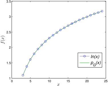
Figure 1. Graph of $\ln(x)$ and $p_{\tiny{G}}(x)$ versus $x$.

Figure 1 shows that the graph of interpolating polynomial $p_{G}(x)$ almost overlapping the graph of $\ln(x)$ in the interval $[3,24]$.

6. Conclusion

In this paper, we have introduced some sequence spaces in bigeometric calculus, determined their $\alpha$-duals and studied matrix transformations of these spaces. We have also derived an interpolating formula in bigeometric calculus and shown some related examples.

References

- [1] Dorota Aniszewska. Multiplicative Runge–Kutta methods. Nonlinear Dynamics, 50(1):265–272, 2007.
- [2] Dorota Aniszewska and Marek Rybaczuk. Analysis of the multiplicative Lorenz system. Chaos, Solitons & Fractals, 25(1):79–90, 2005.
- [3] Agamirza E Bashirov, Emine Mısırlı Kurpınar, and Ali Özyapıcı. Multiplicative calculus and its applications. Journal of Mathematical Analysis and Applications, 337(1):36–48, 2008.
- [4] Khirod Boruah and Bipan Hazarika. Application of geometric calculus in numerical analysis and difference sequence spaces. Journal of Mathematical Analysis and Applications, 449(2):1265–1285, 2017.
- [5] Ahmet Faruk Çakmak and Feyzi Başar. Some new results on sequence spaces with respect to non-Newtonian calculus. Journal of Inequalities and Applications, 2012:228, 2012.
- [6] Ahmet Faruk Çakmak and Feyzi Başar. Some sequence spaces and matrix transformations in multiplicative sense. TWMS Journal of Pure and Applied Mathematics, 6(1):27–37, 2015.
- [7] Tatjana Došenović, Mihai Postolache, and Stojan Radenović. On multiplicative metric spaces: survey. Fixed Point Theory and Applications, 2016:92, 2016.
- [8] Mikail Et. On some generalized Cesàro difference sequence spaces. Istanbul University Fen Fak. Mathematics Dergisi, 55–56:221–229, 1996–1997.
- [9] Mikail Et and Rıfat Çolak. On some generalized difference sequence spaces. Soochow Journal of Mathematics, 21(4):377–386, 1995.
- [10] Michael Grossman. Bigeometric calculus: A system with a scale-free derivative. Archimedes Foundation, 1983.
- [11] Michael Grossman and Robert Katz. Non-Newtonian Calculus: A self-contained, elementary exposition of the authors’ investigations. Lee Press, 1972.
- [12] Uğur Kadak. Determination of the Köthe-Toeplitz duals over the non-Newtonian complex field. The Scientific World Journal, 2014, 2014.
- [13] Uğur Kadak. Cesàro summable sequence spaces over the non-Newtonian complex field. Journal of Probability and Statistics, 2016, 2016.
- [14] Uğur Kadak. On multiplicative difference sequence spaces and related dual properties. Boletim da Sociedade Paranaense de Matemática, 35(3):181–193, 2016.
- [15] Uğur Kadak and Hakan Efe. The construction of Hilbert spaces over the non-Newtonian field. International Journal of Analysis, 2014, 2014.
- [16] Uğur Kadak, Murat Kirişci, and Ahmet Faruk Çakmak. On the classical paranormed sequence spaces and related duals over the non-Newtonian complex field. Journal of Function Spaces, 2015, 2015.
- [17] Shadab Ahmad Khan and Ashfaque A Ansari. Generalized Köthe-Toeplitz dual of some geometric difference sequence spaces. International Journal of Mathematics And its Applications, 4(2):13–22, 2016.
- [18] H Kizmaz. Certain sequence spaces. Canadian Mathematical Bulletin, 24(2):169–176, 1981.
- [19] I J Maddox. Spaces of strongly summable sequences. The Quarterly Journal of Mathematics, 18(1):345–355, 1967.
- [20] C Orhan. Cesàro difference sequence spaces and related matrix transformations. Comm. Fac. Univ. Ankara, Ser. A, 32:55–63, 1983.
- [21] Mustafa Riza, Ali Özyapici, and Emine Misirli. Multiplicative finite difference methods. Quarterly of Applied Mathematics, 67(4):745–754, 2009.
- [22] M Rybaczuk and P Stoppel. The fractal growth of fatigue defects in materials. International Journal of Fracture, 103(1):71–94, 2000.
- [23] Marek Rybaczuk. Critical growth of fractal patterns in biological systems. Acta of Bioengineering and Biomechanics, 1(1):5–9, 1999.
- [24] Cengiz Türkmen and Feyzi Başar. Some basic results on the sets of sequences with geometric calculus. Commun. Fac. Sci. Univ. Ank. Series A1, 61(2):17–34, 2012.