PoPPy: A Point Process Toolbox Based on PyTorch

1 Overview

1.1 What is PoPPy?

PoPPy is a Point Process toolbox based on PyTorch, which achieves flexible designing and efficient learning of point process models. It can be used for interpretable sequential data modeling and analysis, $e.g.$, Granger causality analysis of multivariate point processes, point process-based modeling of event sequences, and event prediction.

1.2 The Goal of PoPPy

Many real-world sequential data are often generated by complicated interactive mechanisms among multiple entities. Treating the entities as events with different discrete categories, we can represent their sequential behaviors as event sequences in continuous time. Mathematically, an event sequence $s$ can be denoted as $\{(t_{i}^{s},c_{i}^{s},f_{c_{i}^{s}})\}_{i=1}^{I_{s}}$, where $t_{i}^{s}$ and $c_{i}^{s}$ are the timestamp and the event type ($i.e.$, the index of entity) of the $i$-th event, respectively. Optionally, each event type may be associated with a feature vector $\bm{f}_{c}\in\mathbb{R}^{D_{c}}$, $c\in\mathcal{C}$, and each event sequence may also have a feature vector $\bm{f}_{s}\in\mathbb{R}^{D_{s}}$, $s\in\mathcal{S}$. Many real-world scenarios can be formulated as event sequences, as shown in Table 1.

Table 1: Typical event sequences in practice.

Scene	Patient admission	Job hopping	Online shopping
Entities (Event types)	Diseases	Companies	Items
Sequences	Patients’ admission records	LinkedIn users’ job history	Buying/rating behaviors
Event feature	Diagnose records	Job descriptions	Item profiles
Sequence feature	Patient profiles	User profiles	User profiles
Task	Build Disease network	Model talent flow	Recommendation system

Given a set of event sequences $\mathcal{S}$, we aim to model the dynamics of the event sequences, capture the interactive mechanisms among different entities, and predict their future behaviors. Temporal point processes provide us with a potential solution to achieve these aims. In particular, a multivariate temporal point process can be represented by a set of counting processes $N=\{N_{c}(t)\}_{c\in\mathcal{C}}$, in which $N_{c}(t)$ is the number of type-$c$ events occurring till time $t$. For each $N_{c}(t)$, the expected instantaneous happening rate of type-$c$ events at time $t$ is denoted as $\lambda_{c}(t)$, which is called “intensity function”:

$$\begin{aligned} \lambda_{c}(t)=\frac{\mathbb{E}[dN_{c}(t)|\mathcal{H}_{t}]}{dt},~{}\mathcal{H}_{t}=\{(t_{i},c_{i})|t_{i}<t,c_{i}\in\mathcal{C}\},\end{aligned}$$ (1)

where $\mathcal{H}_{t}$ represents historical observations before time $t$.

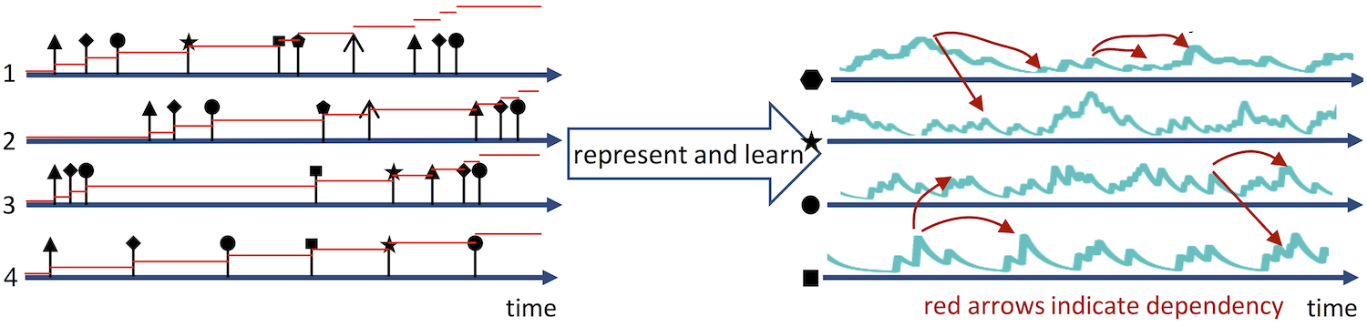
Figure 1: Event sequences and intensity functions.

As shown in Fig. 1, the counting processes can be represented as a set of intensity functions, each of which corresponds to a specific event type. The temporal dependency within the same event type and that across different event types ($i.e.$, the red arrows in Fig. 1) can be captured by choosing particular intensity functions. Therefore, the key points of point process-based sequential data modeling include

1. How to design intensity functions to describe the mechanism behind observed data?

2. How to learn the proposed intensity functions from observed data?

The goal of PoPPy is providing a user-friendly solution to the key points above and achieving large-scale point process-based sequential data analysis, simulation, and prediction.

1.3 Installation of PoPPy

PoPPy is developed on Mac OS 10.13.6 but also tested on Ubuntu 16.04. The installation of PoPPy is straightforward. In particular,

1. Install Anaconda3 and create a conda environment.

2. Install PyTorch0.4 in the environment.

3. Download PoPPy from https://github.com/HongtengXu/PoPPy/ and unzip it to the directory in the environment. The unzipped folder should contain several subfolders, as shown in Fig. 2.

4. Open dev/util.py and change POPPY_PATH to the directory, as shown in Fig. 3.

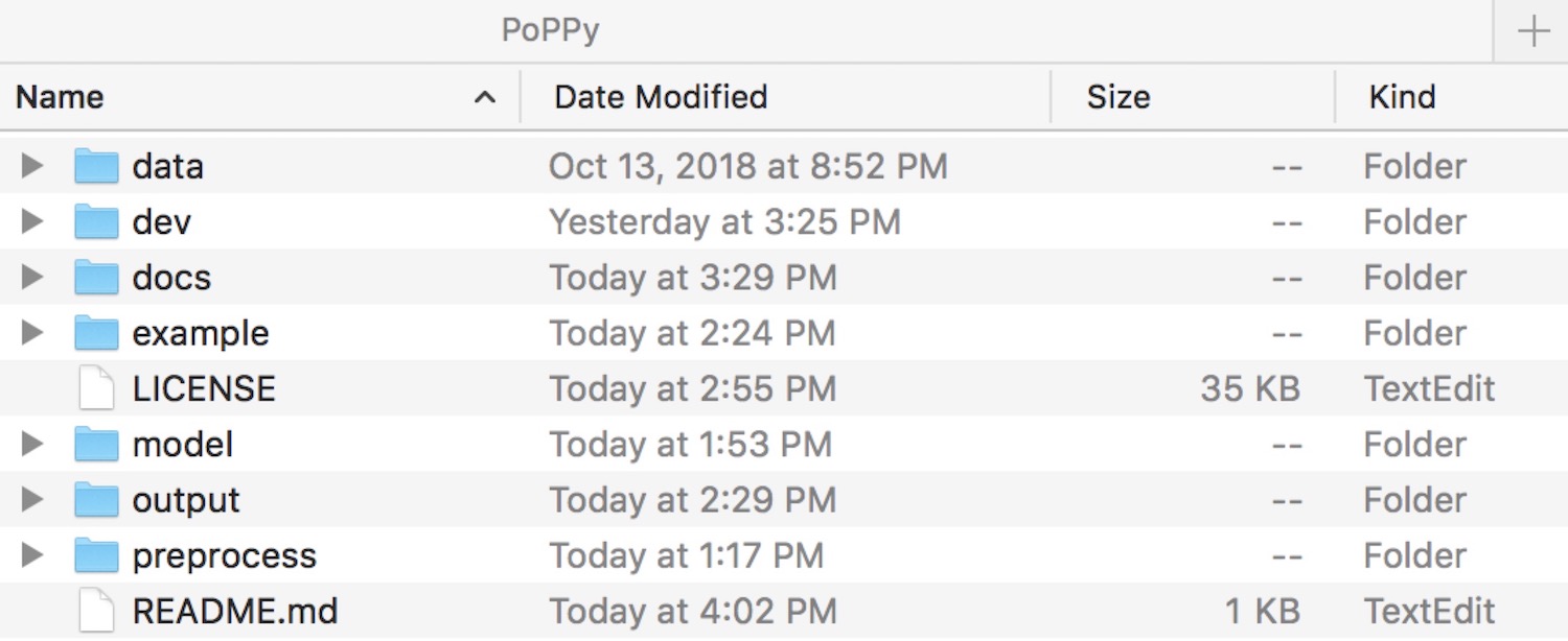
Figure 2: The subfolders in the package of PoPPy.

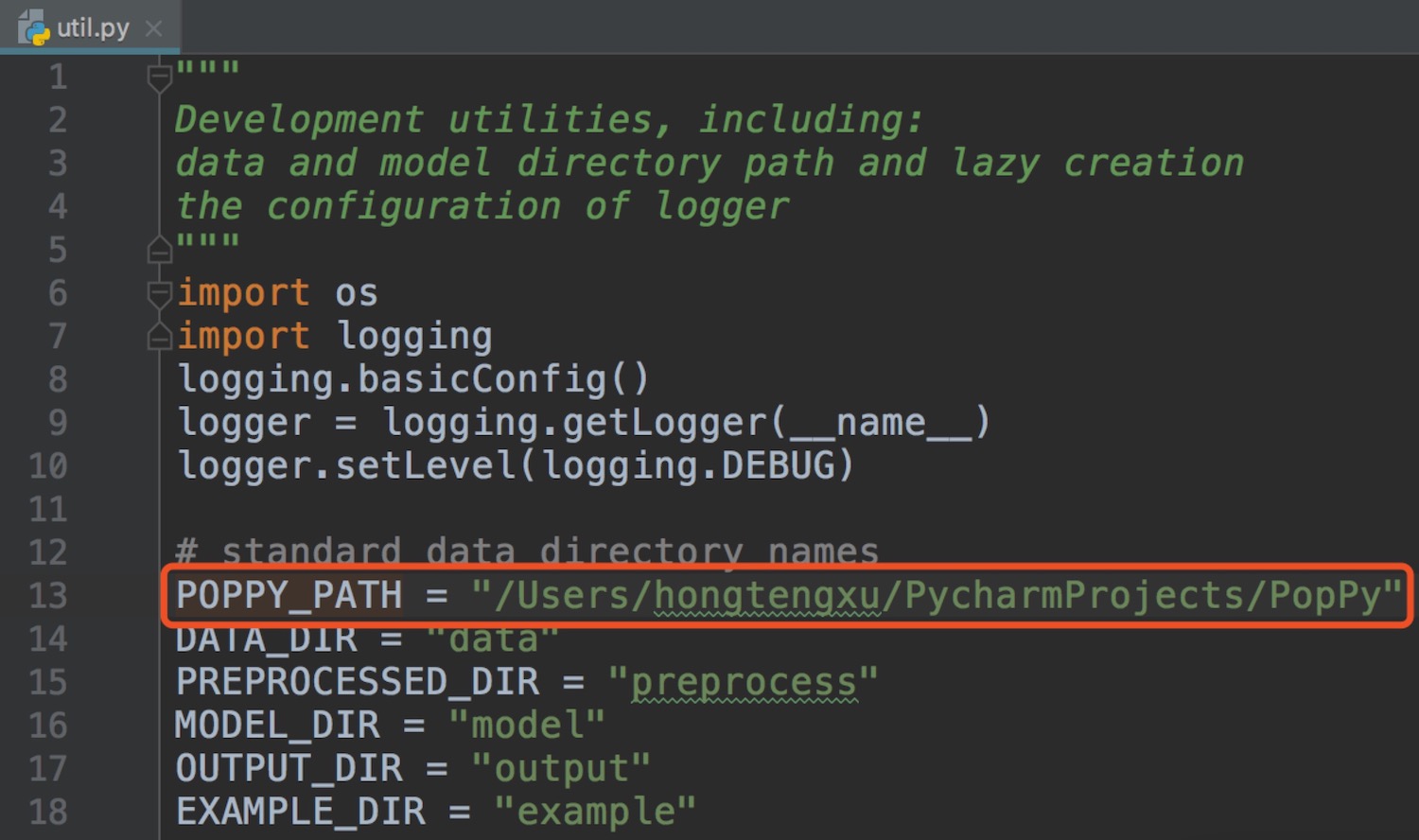
Figure 3: An example of the path of PoPPy.

The subfolders in the package include

• data: It contains a toy dataset in .csv format.

• dev: It contains a util.py file, which configures the path and the logger of the package.

• docs: It contains the tutorial of PoPPy.

• example: It contains some demo scripts for testing the functionality of the package.

• model: It contains the classes of predefined point process models and their modules.

• output: It contains the output files generated by the demo scripts in the example folder.

• preprocess: It contains the classes and the functions of data I/O and preprocessing.

In the following sections, we will introduce the details of PoPPy.

2 Data: Representation and Preprocessing

2.1 Representations of Event Sequences

PoPPy represents observed event sequences as a nested dictionary. In particular, the proposed database has the following structure:

⬇

database = {

’event_features’ : None or (De, C) float array of event features,

C is the number of event types.

De is the dimension of event feature.

’type2idx’ : a Dict = {’event_name’: event_index}

’idx2type’ : a Dict = {event_index: ’event_name’}

’seq2idx’ : a Dict = {’seq_name’: seq_index}

’idx2seq’ : a Dict = {seq_index: ’seq_name’}

’sequences’ : a List = [seq_1, seq_2, ..., seq_N].

}

For the i-th sequence:

seq_i = {

’times’ : (N,) float array of timestamps,

N is the number of events.

’events’ : (N,) int array of event types.

’seq_feature’ : None or (Ds,) float array of sequence feature.

Ds is the dimension of sequence feature

’t_start’ : a float number, the start timestamp of the sequence.

’t_stop’ : a float number, the stop timestamp of the sequence.

’label’ : None or int/float number, the labels of the sequence

}

PoPPy provides three functions to load data from .csv file and convert it to the proposed database.

2.1.1 preprocess.DataIO.load_sequences_csv

This function loads event sequences and converts them to the proposed database. The IO and the description of this function are shown in Fig. 4.

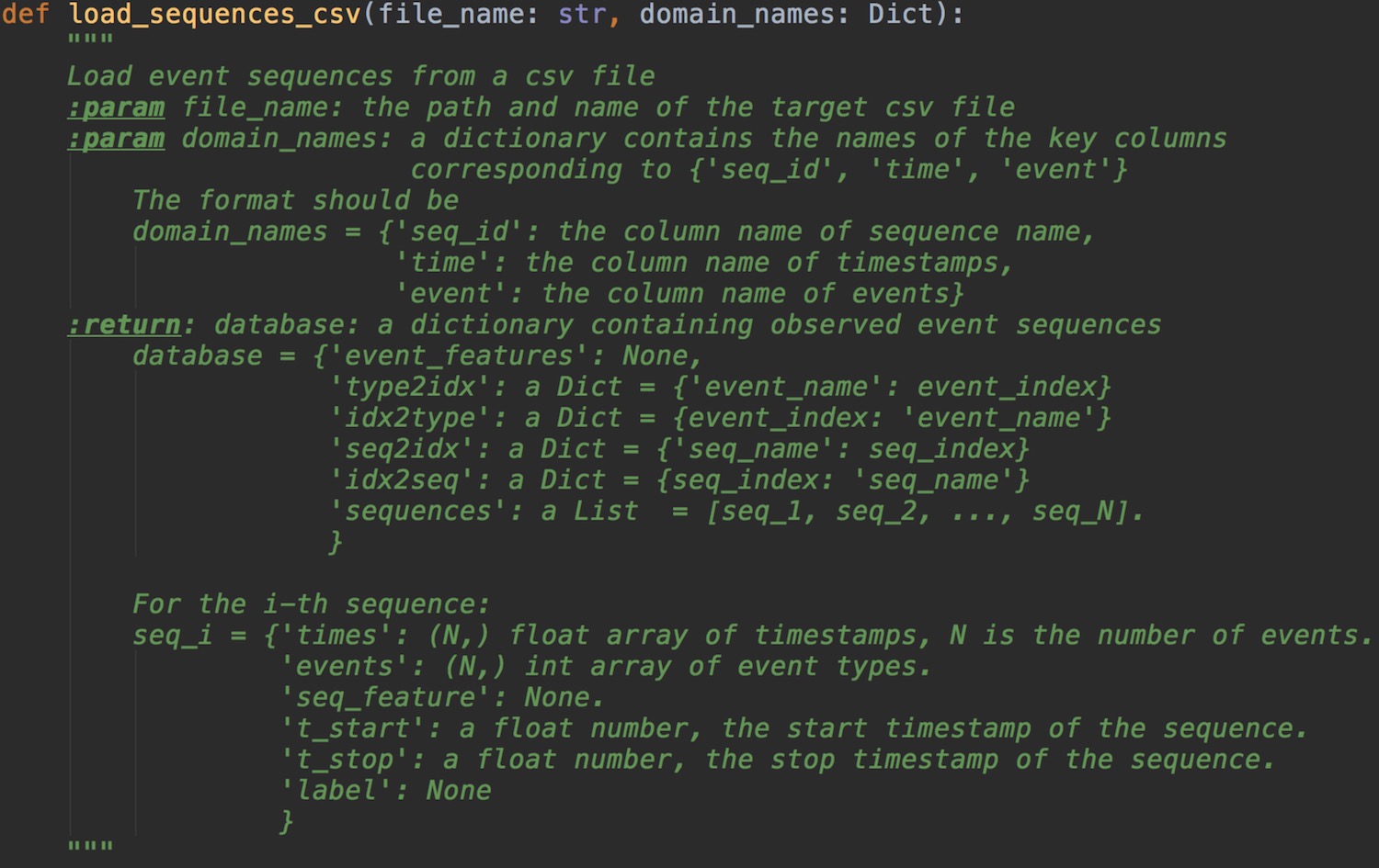
Figure 4: The description of load_sequences_csv.

For example, the Linkedin.csv file in the folder data records a set of linkedin users’ job-hopping behaviors among different companies, whose format is shown in Fig. 5.

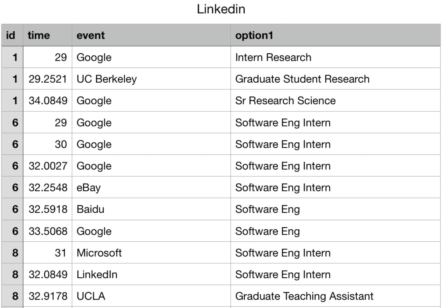
Figure 5: Some rows of Linkedin.csv.

Here, the column id corresponds to the names of sequences ($i.e.$ the index of users), the column time corresponds to the timestamps of events ($i.e.$ the ages that the users start to work), and the column event corresponds to the event types ($i.e.$, the companies). Therefore, we can define the input domain_names as

⬇

domain_names = {

’seq_id’ : ’id’,

’time’ : ’time’,

’event’ : ’event’

}

and database = load_sequences_csv(’Linkedin.csv’, domain_names).

Note that the database created by load_sequences_csv() does not contain event features and sequence features, whose values in database are None. PoPPy supports to load categorical or numerical features from .csv files, as shown below.

2.1.2 preprocess.DataIO.load_seq_features_csv

This function loads sequence features from a .csv file and import them to the proposed database. The IO and the description of this function are shown in Fig. 6.

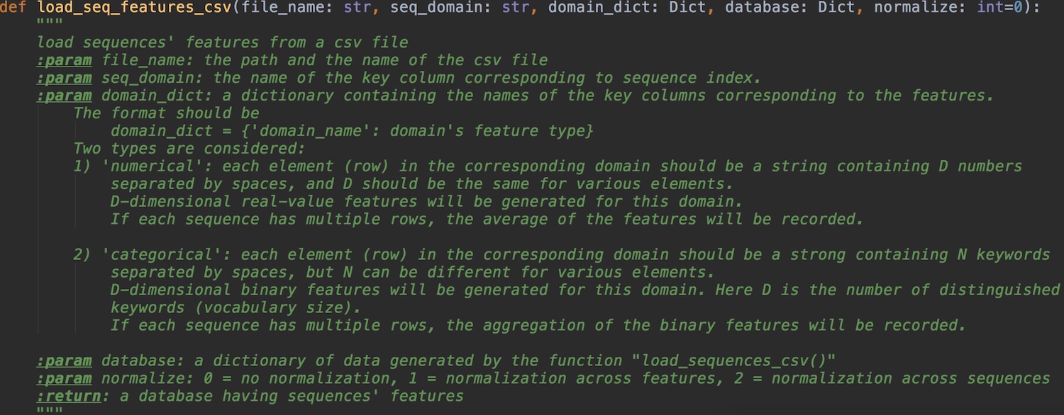
Figure 6: The description of load_seq_features_csv.

Take the Linkedin.csv file as an example. Suppose that we have already create database by the function load_sequences_csv, and we want to take the column option1 ($i.e.$, the job titles that each user had) as the categorical features of event sequences. We should have

⬇

domain_names = {

’option1’ : ’categorical’

}

database = load_seq_features_csv(

file_name = ’Linkedin.csv’,

seq_domain = ’seq_id’,

domain_dict = domain_names,

database = database)

Here the input normalize is set as default $0$, which means that the features in database[’sequences’][i][’seq_feature’], $i=1,...,|\mathcal{S}|$, are not normalized.

2.1.3 preprocess.DataIO.load_event_features_csv

This function loads event features from a .csv file and import them to the proposed database. The IO and the description of this function are shown in Fig. 7.

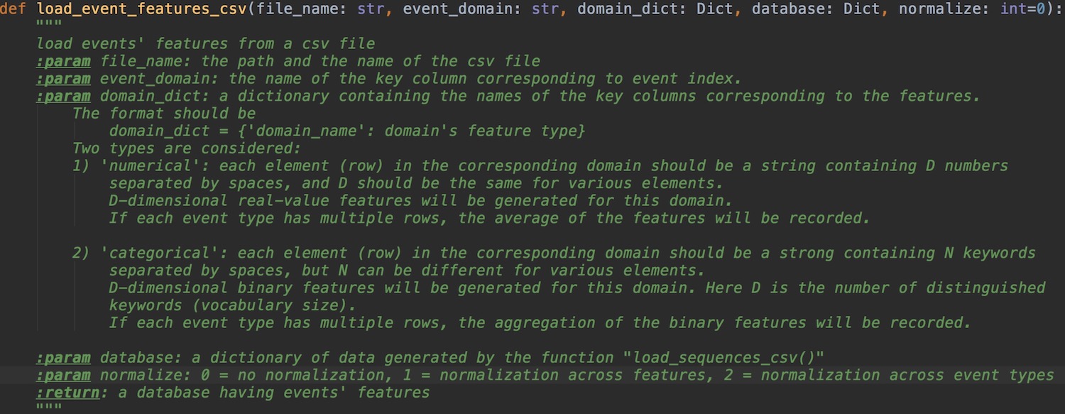
Figure 7: The description of load_event_features_csv.

Similarly, if we want to take the column option1 in Linkedin.csv as the categorical features of event types, we should have

⬇

domain_names = {

’option1’ : ’categorical’

}

database = load_event_features_csv(

file_name = ’Linkedin.csv’,

event_domain = ’event’,

domain_dict = domain_names,

database = database)

2.2 Operations for Data Preprocessing

Besides necessary sequence/feature loaders and converters mentioned above, PoPPy contains multiple useful functions and classes for data preprocessing, including sequence stitching, superposing, aggregating, and batch sampling. Fig. 8 illustrates the corresponding data operations.

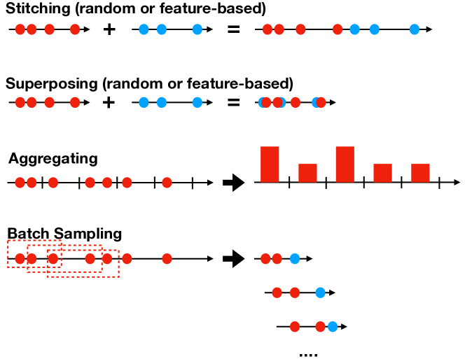
Figure 8: The illustration of four data operations.

2.2.1 preprocess.DataOperation.stitching

This function stitches the sequences in two database randomly or based on their seq_feature and time information (t_start, t_stop). Its description is shown in Fig. 9.

When method = ’random’, for each sequence in database1 the function randomly selects a sequence in database2 as its follower and stitches them together. When method = ’feature’, the similarity between the sequence in database1 and that in database2 is defined by the multiplication of a temporal Gaussian kernel and a sequence feature’s Gaussian kernel, and the function selects the sequence in database2 yielding to a distribution defined by the similarity. The stitching method has been proven to be useful for enhancing the robustness of learning results, especially when the training sequences are very short [9, 4].

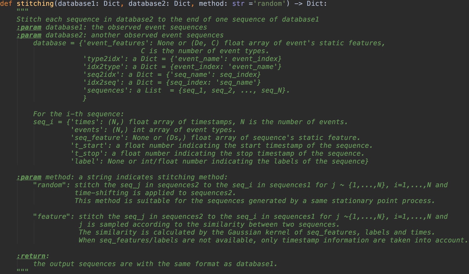
Figure 9: The description of stitching.

2.2.2 preprocess.DataOperation.superposing

This function superposes the sequences in two database randomly or based on their seq_feature and time information (t_start, t_stop). Its description is shown in Fig. 10.

When method = ’random’, for each sequence in database1 the function randomly selects a sequence in database2 and superposes them together. When method = ’feature’, the similarity between the sequence in database1 and that in database2 is defined by the multiplication of a temporal Gaussian kernel and a sequence feature’s Gaussian kernel, and the function selects the sequence in database2 yielding to a distribution defined by the similarity.

Similar to the stitching operation, the superposing method has been proven to be useful for learning linear Hawkes processes robustly. However, it should be noted that different from stitching operation, which stitches similar sequences with a high probability, the superposing process would like to superpose the dissimilar sequences with a high chance. The rationality of such an operation can be found in my paper [8, 5].

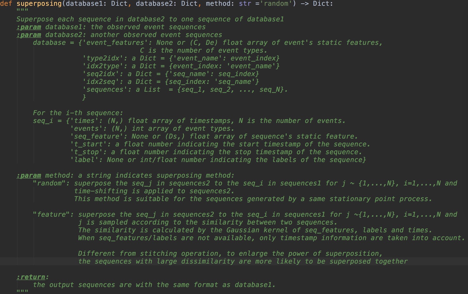
Figure 10: The description of superposing.

2.2.3 preprocess.DataOperation.aggregating

This function discretizes each event sequence into several bins and counts the number of events with specific types in each bin. Its description is shown in Fig. 11.

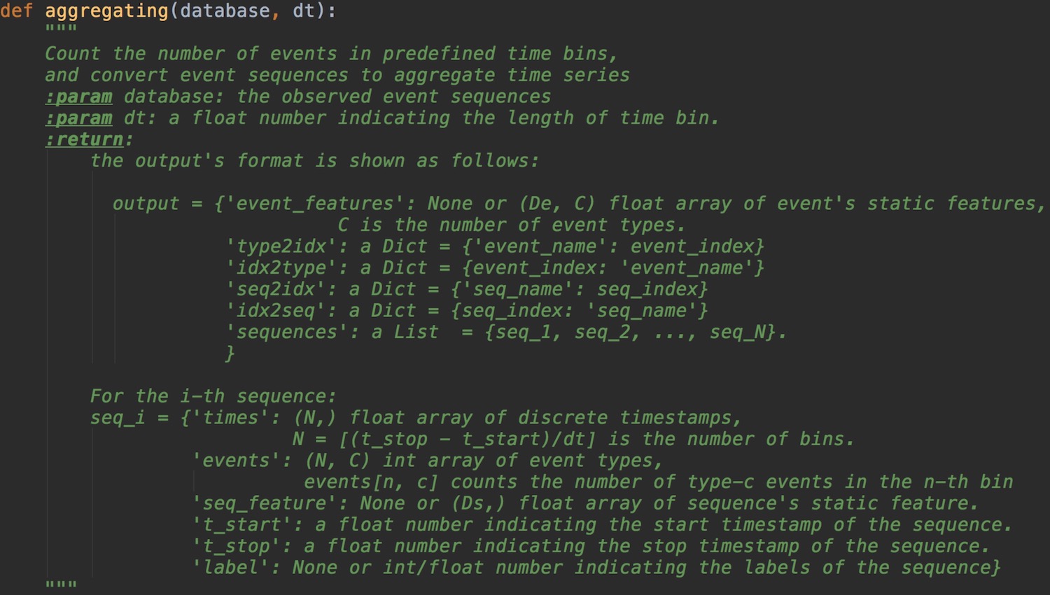
Figure 11: The description of aggregate.

2.2.4 preprocess.DataOperation.EventSampler

This class is a subclass of torch.utils.data.Dataset, which samples batches from database. For each sample in the batch, an event ($i.e.$, its event type and timestamp) and its history with length memorysize ($i.e.$, the last memorysize events and their timestamps) are recorded. If the features of events (or sequences) are available, the sample will record these features as well.

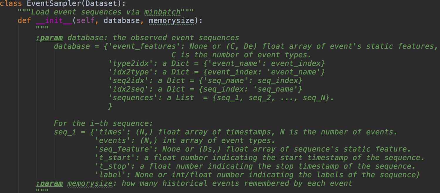
Figure 12: The description of EventSampler.

3 Temporal Point Process Models

3.1 Modular design of point process model

PoPPy applies a flexible strategy to build point process’s intensity functions from interpretable modules. Such a modular design strategy is very suitable for the Hawkes process and its variants. Fig. 13 illustrates the proposed modular design strategy. In the following sections, we take the Hawkes process and its variants as examples and introduce the modules ($i.e.$, the classes) in PoPPy.

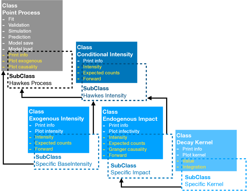
Figure 13: An illustration of proposed modular design strategy. Each color block represents a class with some functions. For each block, the dotted frame represents one of its subclass, which inherits some functions (the white ones) while overrides some others or creates new ones (the yellow ones). The black arrow means that the destination class will call the instance of the source class as input.

3.2 model.PointProcess.PointProcessModel

This class contains basic functions of a point process model, including

• fit: learn model’s parameters given training data. It description is shown in Fig. 14

  

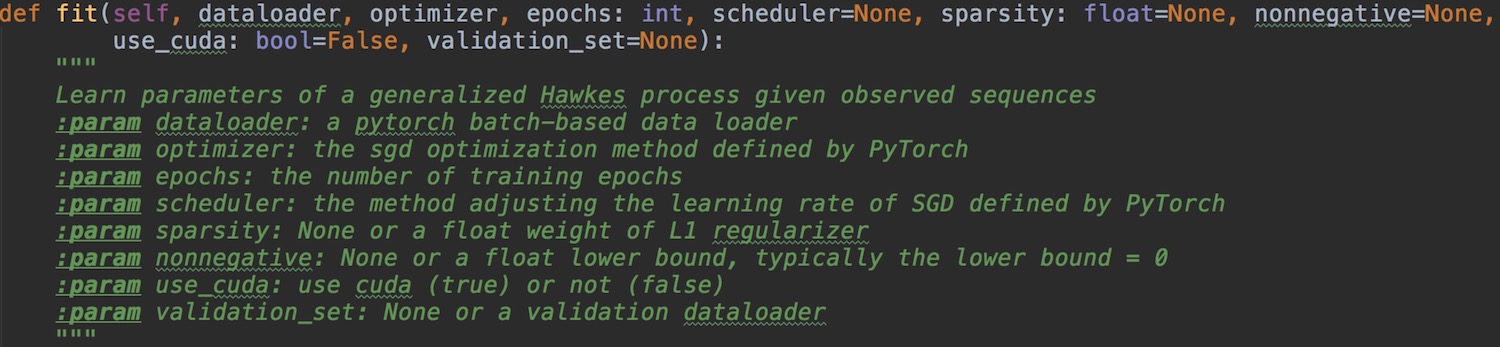
  Figure 14: The description of fit.

• validation: test model given validation data. It description is shown in Fig. 15

  

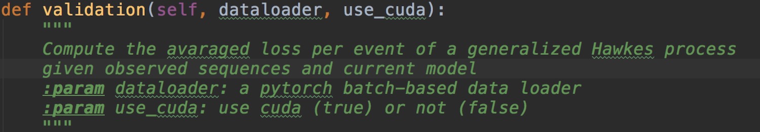
  Figure 15: The description of validation.

• simulation: simulate new event sequences from scratch or following observed sequences by Ogata’s thinning algorithm [3]. It description is shown in Fig. 16

  

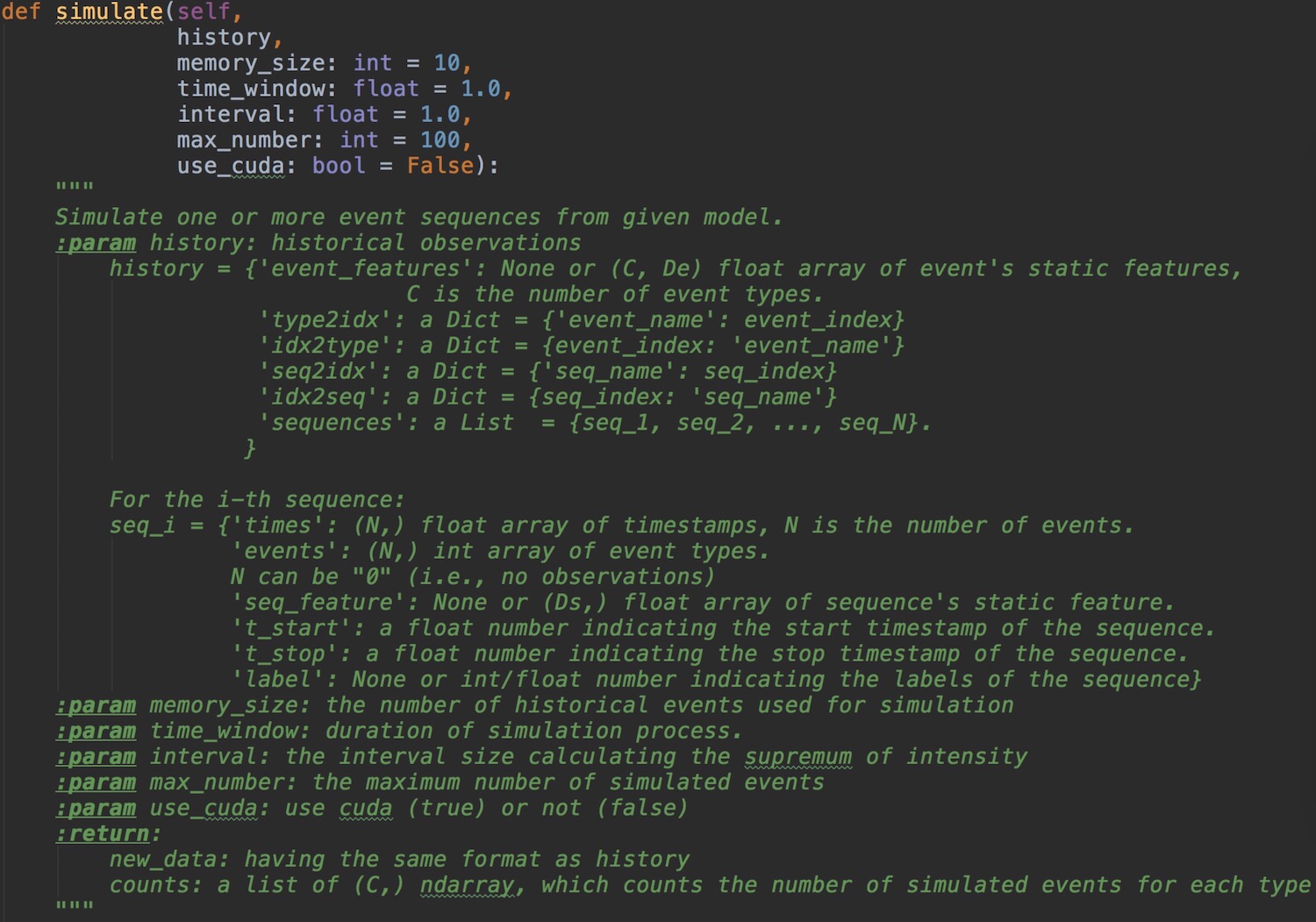
  Figure 16: The description of simulate.

• prediction: predict expected counts of the events in the target time inteveral given learned model and observed sequences. It description is shown in Fig. 17

  

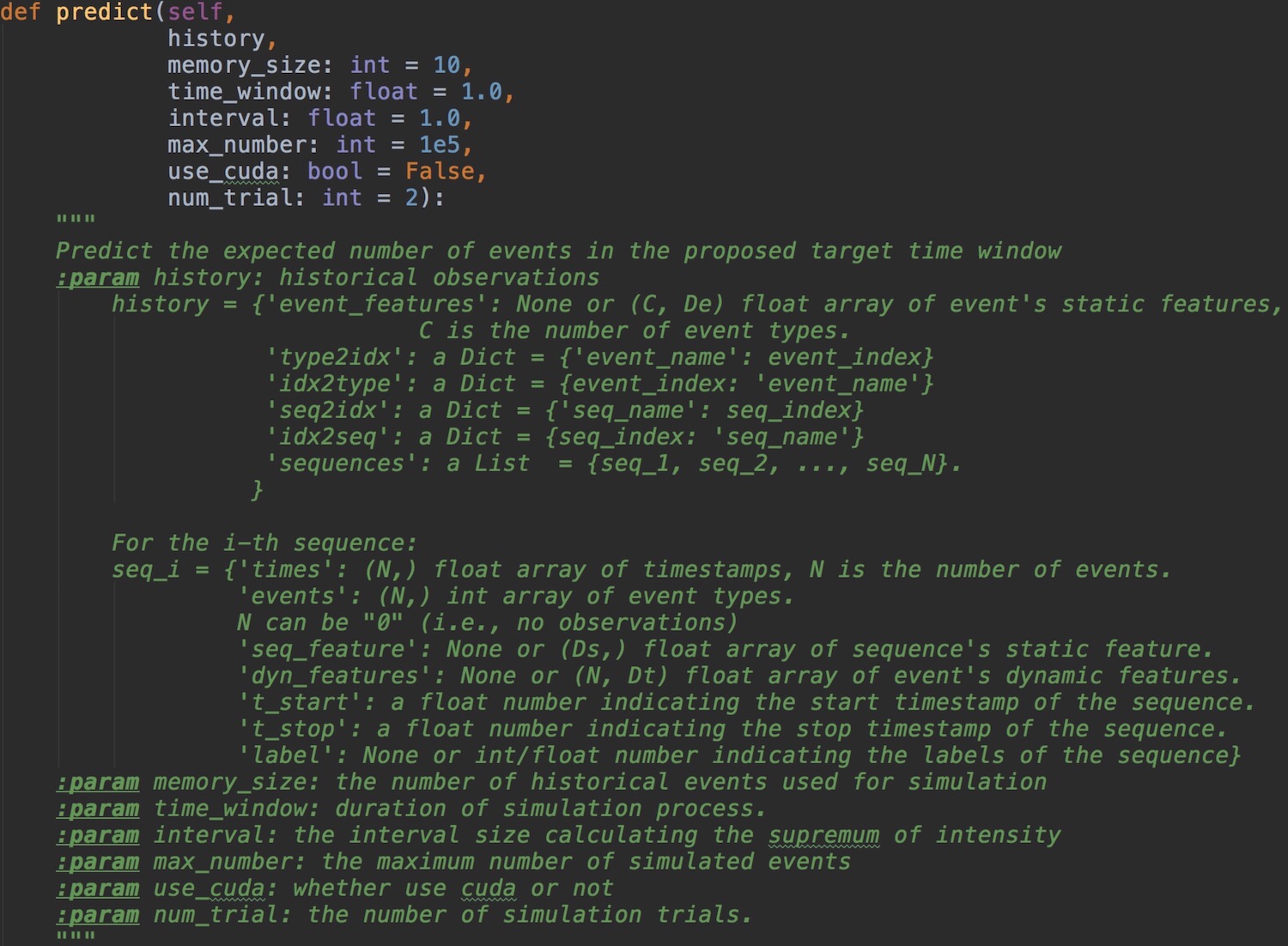
  Figure 17: The description of predict.

• model_save: save model or save its parameters. It description is shown in Fig. 18

  

  Figure 18: The description of model_save.

• model_load: load model or load its parameters. It description is shown in Fig. 19

  

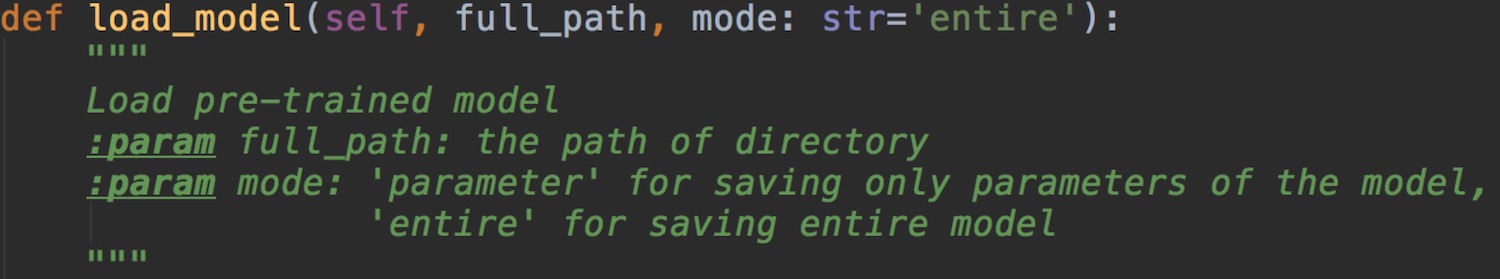
  Figure 19: The description of model_load.

• print_info: print basic information of model

• plot_exogenous: print exogenous intensity.

In PoPPy, the instance of this class implements an inhomogeneous Poisson process, in which the exogenous intensity is used as the intensity function.

An important subclass of this class is model.HawkesProcess.HawkesProcessModel. This subclass inherits most of the functions above except print_info and plot_exogenous. Additionally, because the Hawkes process considers the triggering patterns among different event types, this subclass has a new function plot_causality, which plots the adjacency matrix of the event types’ Granger causality graph. The typical visualization results of the exogenous intensity of different event types and the Granger causality among them are shown in Fig. 20.

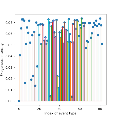
(a) exogenous intensity

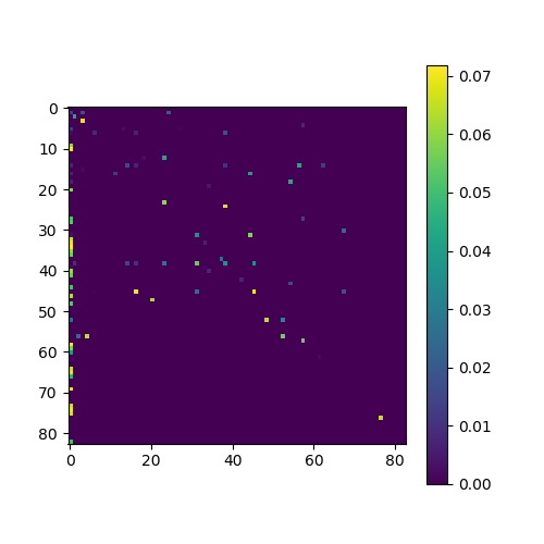
(b) Granger causality

Figure 20: Typical visualization results.

Compared with its parant class, model.HawkesProcess.HawkesProcessModel uses a specific intensity function, which is defined in the class model.HawkesProcess.HawkesProcessIntensity.

3.3 model.HawkesProcess.HawkesProcessIntensity

This class inherits the functions in torch.nn.Module. It defines the intensity function of a generalized Hawkes process, which contains the following functions:

• print_info: print the basic information of the intensity function.

• intensity: calculate $\lambda_{c_{i}}(t_{i})$ of the $i$-th sample in the batch sampled by EventSampler.

• expected_counts: calculate $\int_{t_{i-1}}^{t_{i}}\lambda_{c}(s)ds$ for $c\in\mathcal{C}$ and for the $i$-th sample in the batch.

• forward: override the forward function in torch.nn.Module. It calculates $\lambda_{c_{i}}(t_{i})$ and $\int_{t_{i-1}}^{t_{i}}\lambda_{c}(s)ds$ for $c\in\mathcal{C}$ for SGD.

Specifically, the intensity function of type-$c$ event at time $t$ is defined as

$$\begin{aligned} \lambda_{c}(t)&=g_{\lambda}\left(\underbrace{\mu_{c}(\bm{f}_{c},\bm{f}_{s})}_{\mbox{exogenous intensity}}+\underbrace{\sum_{t_{i}<t}\phi_{cc_{i}}(t-t_{i},\bm{f}_{c},\bm{f}_{c_{i}})}_{\mbox{endogeneous impact}}\right)\\ &=\mu_{c}(\bm{f}_{c},\bm{f}_{s})+\sum_{t_{i}<t}\sum_{m=1}^{M}\alpha_{cc_{i}m}(\bm{f}_{c},\bm{f}_{c_{i}})\kappa_{m}(t-t_{i}).\end{aligned}$$ (2)

Here, the intensity function is consist of two parts:

• Exogenous intensity $\mu_{c}(\bm{f}_{c},\bm{f}_{s})$: it is independent with time, which measures the intensity contributed by the intrinsic properties of sequence and event type.

• Endogenous impact $\sum_{t_{i}<t}\phi_{cc_{i}}(t-t_{i},\bm{f}_{c},\bm{f}_{c_{i}})$: it sums up the influences of historical events quantitatively via impact functions $\{\phi_{cc^{\prime}}(t)\}_{c,c^{\prime}\in\mathcal{C}}$, which measures the intensity contributed by the historical observations.

Furthermore, the impact function is decomposed with the help of basis representation, where $\kappa_{m}(t)$ is called the $m$-th decay kernel and $\alpha_{cc_{i}m}(\bm{f}_{c},\bm{f}_{c_{i}})$ is the corresponding coefficient.

$g_{\lambda}(\cdot)$ is an activation function, which can be

• Identity: $g(x)=x$.

• ReLU: $g(x)=\max\{x,0\}$.

• Softplus: $g(x)=\frac{1}{\beta}\log(1+\exp(-\beta x))$.

PoPPy provides multiple choices to implement various intensity functions — each module can be parametrized in different ways.

3.3.1 model.ExogenousIntensity.BasicExogenousIntensity

This class and its subclasses in model.ExogenousIntensityFamily implements several models of exogenous intensity, as shown in Table 2.

Table 2: Typical models of exogenous intensity.

Class	Formulation
ExogenousIntensity.BasicExogenousIntensity	$\mu_{c}(\bm{f}_{c},\bm{f}_{s})=\mu_{c}$
ExogenousIntensityFamily.NaiveExogenousIntensity	$\mu_{c}(\bm{f}_{c},\bm{f}_{s})=g(\mu_{c})$
ExogenousIntensityFamily.LinearExogenousIntensity	$\mu_{c}(\bm{f}_{c},\bm{f}_{s})=g(\bm{w}_{c}^{\top}\bm{f}_{s})$
ExogenousIntensityFamily.NeuralExogenousIntensity	$\mu_{c}(\bm{f}_{c},\bm{f}_{s})=NN(\bm{f}_{c},\bm{f}_{s})$

Here, the activation function $g(\cdot)$ is defined as aforementioned $g_{\lambda}$.

Note that the last two models require event and sequence features as input. When they are called while the features are not given, PoPPy will add one more embedding layer to generate event/sequence features from their index, and learn this layer during training.

3.3.2 model.EndogenousImpact.BasicEndogenousImpact

This class and its subclasses in model.EndogenousImpactFamily implement several models of the coefficients of the impact function, as shown in Table 3.

Table 3: Typical models of endogenous impact’s coefficient.

Class	Formulation
EndogenousImpact.BasicEndogenousImpact	$\alpha_{cc^{\prime}m}(\bm{f}_{c},\bm{f}_{c^{\prime}})=\alpha_{cc^{\prime}m}$
EndogenousImpactFamily.NaiveEndogenousImpact	$\alpha_{cc^{\prime}m}(\bm{f}_{c},\bm{f}_{c^{\prime}})=g(\alpha_{cc^{\prime}m})$
EndogenousImpactFamily.FactorizedEndogenousImpact	$\alpha_{cc^{\prime}m}(\bm{f}_{c},\bm{f}_{c^{\prime}})=g(\bm{u}_{cm}^{\top}\bm{v}_{c^{\prime}m})$
EndogenousImpactFamily.LinearEndogenousImpact	$\alpha_{cc^{\prime}m}(\bm{f}_{c},\bm{f}_{c^{\prime}})=g(\bm{w}_{cm}^{\top}\bm{f}_{c^{\prime}})$
EndogenousImpactFamily.BiLinearEndogenousImpact	$\alpha_{cc^{\prime}m}(\bm{f}_{c},\bm{f}_{c^{\prime}})=g(\bm{f}_{c}^{\top}\bm{W}_{m}\bm{f}_{c^{\prime}})$

Here, the activation function $g(\cdot)$ is defined as aforementioned $g_{\lambda}$.

Note that the last two models require event and sequence features as input. When they are called while the features are not given, PoPPy will add one more embedding layer to generate event/sequence features from their index, and learn this layer during training.

3.3.3 model.DecayKernel.BasicDecayKernel

This class and its subclasses in model.DecayKernelFamily implements several models of the decay kernel, as shown in Table 4.

Table 4: Typical models of decay kernel.

Class	$M$	Formulation
DecayKernelFamily.ExponentialKernel [13]	1	$\kappa(t)=\begin{cases}\omega\exp(-\omega(t-\delta)),&t\geq\delta,\\ 0,&t<\delta\end{cases}$
DecayKernelFamily.RayleighKernel	1	$\kappa(t)=\omega t\exp(-\omega t^{2}/s)$
DecayKernelFamily.GaussianKernel	1	$\kappa(t)=\frac{1}{\sqrt{2\pi}\sigma}\exp(-\frac{t^{2}}{2\sigma^{2}})$
DecayKernelFamily.PowerlawKernel [12]	1	$\kappa(t)=\begin{cases}(\omega-1)\delta^{\omega-1}t^{-\omega},&x\geq\delta,\\ (\omega-1)/\delta,&0<x<\delta\end{cases}$
DecayKernelFamily.GateKernel	1	$\kappa(t)=\frac{1}{\delta},~{}t\in[\omega,\omega+\delta]$
DecayKernelFamily.MultiGaussKernel [6]	>1	$\kappa_{m}(t)=\frac{1}{\sqrt{2\pi}\sigma_{m}}\exp(-\frac{(t-t_{m})^{2}}{2\sigma_{m}^{2}})$

Fig. 21 visualizes some examples.

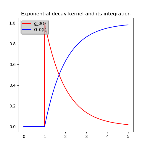
(a) Exponential kernel

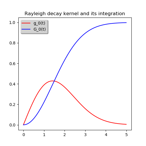
(b) Rayleigh kernel

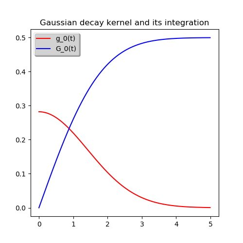
(c) Gaussian kernel

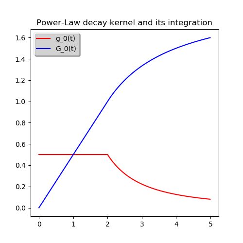
(d) Powerlaw kernel

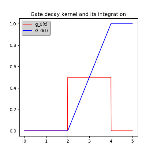
(e) Gate kernel

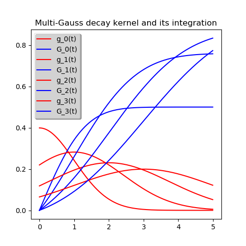
(f) Multi-Gaussian kernel

Figure 21: Examples of decay kernels and their integration values.

4 Learning Algorithm

4.1 Loss functions

With the help of PyTorch, PoPPy learns the point process models above efficiently by stochastic gradient descent on CPU or GPU [2]. Different from existing point process toolboxes, which mainly focuses on the maximum likelihood estimation of point process models, PoPPy integrates three loss functions to learn the models, as shown in Table 5.

Table 5: A list of loss functions.

Maximum Likelihood Estimation [13, 6]

- Class: OtherLayers.MaxLogLike

- Formulation: $L(\theta)=-\sum_{i\in\mathcal{D}}\left(\log\lambda_{c_{i}}(t_{i})-\sum_{c\in\mathcal{C}}\int_{t_{i-1}}^{t_{i}}\lambda_{c}(s)ds\right)$

Least Square Estimation [8, 7]

- Class: OtherLayers.LeastSquare

- Formulation: $L(\theta)=\sum_{i\in\mathcal{D}}\|\int_{t_{i-1}}^{t_{i}}\bm{\lambda}(s)ds-\bm{1}_{c_{i}}\|_{2}^{2}$

Conditional Likelihood Estimation [10]

- Class: OtherLayers.CrossEntropy

- Formulation: $L(\theta)=-\sum_{i\in\mathcal{D}}\log p(c_{i}|t_{i},\mathcal{H}_{i})=-\sum_{i\in\mathcal{D}}\log softmax\left(\int_{t_{i-1}}^{t_{i}}\bm{\lambda}(s)ds\right).$

Here $\bm{\lambda}(t)=[\lambda_{1}(t),...,\lambda_{|\mathcal{C}|}(t)]$ and $\bm{1}_{c}$ is an one-hot vector whose the $c$-th element is 1.

4.2 Stochastic gradient decent

All the optimizers and the learning rate schedulers in PyTorch are applicable to PoPPy. A typical configuration is using Adam + Exponential learning rate decay strategy, which should achieve good learning results in most situations. The details can be found in the demo scripts in the folder example.

Trick: Although most of the optimizers are applicable, generally, Adam achieves the best performance in our experiments [2].

4.3 Optional regularization

Besides the L2-norm regularizer in PyTorch, PoPPy provides two more regularizers when learning models.

1. Sparsity: L1-norm of model’s parameters can be applied to the models, which helps to learn structural parameters.

2. Nonnegativeness: If it is required, PoPPy can ensure the parameters to be nonnegative during training.

Trick: When the activation function of impact coefficient is softplus, you’d better close the nonnegative constraint by setting the input nonnegative of the function fit as None.

5 Examples

As a result, using PoPPy, users can build their own point process models by combining different modules with high flexibility. As shown in Fig. 22, Each point process model can be built by selecting different modules and combining them. The red dots represent the module with learnable parameters, the blue dots represent the module without parameters, and the green dots represent loss function modules. Moreover, users can add their own modules and design specific point process models for their applications quickly, as long as the new classes override the corresponding functions.

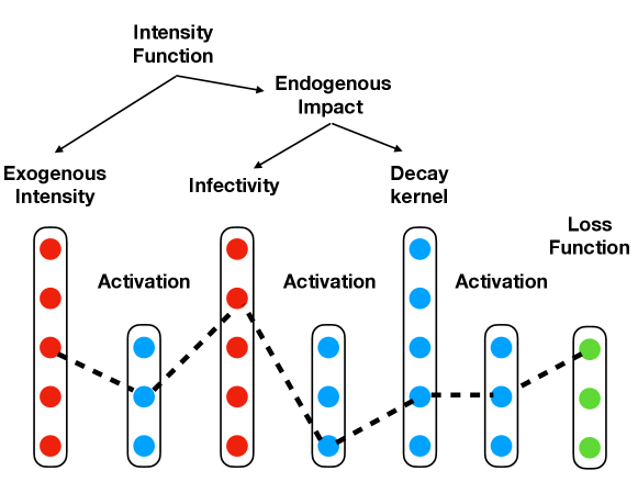
Figure 22: Illustration the contruction of a point process model.

Finally, we list some typical models implemented by PoPPy in Table 6.

Table 6: Typical models implemented by PoPPy.

Model	Linear Hawkes process [13]
Exogenous Intensity	NaiveExogenousIntensity
Endogenous Impact	NavieEndogenousImpact
Decay Kernel	ExponentialKernel
Activation $g_{\lambda}$	Identity
Loss	MaxLogLike
Model	Linear Hawkes process [6, 5]
Exogenous Intensity	NaiveExogenousIntensity
Endogenous Impact	NavieEndogenousImpact
Decay Kernel	MultiGaussKernel
Activation $g_{\lambda}$	Identity
Loss	MaxLogLike
Model	Linear Hawkes process [8]
Exogenous Intensity	NaiveExogenousIntensity
Endogenous Impact	NavieEndogenousImpact
Decay Kernel	MultiGaussKernel
Activation $g_{\lambda}$	Identity
Loss	LeastSquares
Model	Factorized point process [7]
Exogenous Intensity	LinearExogenousIntensity
Endogenous Impact	FactorizedEndogenousImpact
Decay Kernel	ExponentialKernel
Activation $g_{\lambda}$	Identity
Loss	LeastSquares
Model	Semi-Parametric Hawkes process [1]
Exogenous Intensity	LinearExogenousIntensity
Endogenous Impact	NavieEndogenousImpact
Decay Kernel	MultiGaussKernel
Activation $g_{\lambda}$	Identity
Loss	MaxLogLike
Model	Parametric self-correcting process [11]
Exogenous Intensity	LinearExogenousIntensity
Endogenous Impact	LinearEndogenousImpact
Decay Kernel	GateKernel
Activation $g_{\lambda}$	Softplus
Loss	MaxLogLike
Model	Mutually-correcting process [10]
Exogenous Intensity	LinearExogenousIntensity
Endogenous Impact	LinearEndogenousImpact
Decay Kernel	GaussianKernel
Activation $g_{\lambda}$	Softplus
Loss	CrossEntropy

References

- [1] M. Engelhard, H. Xu, L. Carin, J. A. Oliver, M. Hallyburton, and F. J. McClernon. Predicting smoking events with a time-varying semi-parametric hawkes process model. arXiv preprint arXiv:1809.01740, 2018.
- [2] H. Mei and J. M. Eisner. The neural hawkes process: A neurally self-modulating multivariate point process. In Advances in Neural Information Processing Systems, pages 6754–6764, 2017.
- [3] Y. Ogata. On lewis’ simulation method for point processes. IEEE Transactions on Information Theory, 27(1):23–31, 1981.
- [4] H. Xu, L. Carin, and H. Zha. Learning registered point processes from idiosyncratic observations. In International Conference on Machine Learning, 2018.
- [5] H. Xu, X. Chen, and L. Carin. Superposition-assisted stochastic optimization for hawkes processes. arXiv preprint arXiv:1802.04725, 2018.
- [6] H. Xu, M. Farajtabar, and H. Zha. Learning granger causality for hawkes processes. In International Conference on Machine Learning, pages 1717–1726, 2016.
- [7] H. Xu, D. Luo, and L. Carin. Online continuous-time tensor factorization based on pairwise interactive point processes. In Proceedings of the 27th International Conference on Artificial Intelligence. AAAI Press, 2018.
- [8] H. Xu, D. Luo, X. Chen, and L. Carin. Benefits from superposed hawkes processes. In International Conference on Artificial Intelligence and Statistics, pages 623–631, 2018.
- [9] H. Xu, D. Luo, and H. Zha. Learning hawkes processes from short doubly-censored event sequences. In International Conference on Machine Learning, pages 3831–3840, 2017.
- [10] H. Xu, W. Wu, S. Nemati, and H. Zha. Patient flow prediction via discriminative learning of mutually-correcting processes. IEEE Transactions on Knowledge and Data Engineering, 29(1):157–171, 2017.
- [11] H. Xu, Y. Zhen, and H. Zha. Trailer generation via a point process-based visual attractiveness model. In Proceedings of the 24th International Conference on Artificial Intelligence, pages 2198–2204. AAAI Press, 2015.
- [12] Q. Zhao, M. A. Erdogdu, H. Y. He, A. Rajaraman, and J. Leskovec. Seismic: A self-exciting point process model for predicting tweet popularity. In Proceedings of the 21th ACM SIGKDD International Conference on Knowledge Discovery and Data Mining, pages 1513–1522. ACM, 2015.
- [13] K. Zhou, H. Zha, and L. Song. Learning social infectivity in sparse low-rank networks using multi-dimensional hawkes processes. In Artificial Intelligence and Statistics, pages 641–649, 2013.