SHAPE DERIVATIVES

Edward Anderson^∗

Shape Theory, together with Shape-and-Scale Theory, comprise Relational Theory. This consists of $N$-point models on a manifold $\mathfrak{M}$, for which some geometrical automorphism group $\mathfrak{g}$ is regarded as meaningless and is thus quotiented out from the $N$-point model’s product space $\mbox{\Large$\times$}_{I=1}^{N}\mbox{\boldmath$\mathfrak{M}$}$. Each such model has an associated function space of preserved quantities, solving the PDE system for zero brackets with the sums over $N$ of each of $\mathfrak{g}$’s generators. These are smooth functions of the $N$-point geometrical invariants. Each $(\mbox{\boldmath$\mathfrak{M}$},\mbox{\Large$\mathfrak{g}$})$ pair has moreover a ‘minimal nontrivially relational unit’ value of $N$; we now show that relationally-invariant derivatives can be defined on these, yielding the titular notions of shape(-and-scale) derivatives. We obtain each by Taylor-expanding a functional version of the underlying geometrical invariant, and isolating a shape-independent derivative factor in the nontrivial leading-order term. We do this for translational, dilational, dilatational and projective geometries in 1-$d$, the last of which gives a shape-theoretic rederivation of the Schwarzian derivative. We next phrase and solve the ODEs for zero and constant values of each derivative. We then consider translational, dilational, rotational, rotational-and-dilational, Euclidean and equi-top-form (alias unimodular affine) cases in $\geq 2$-$d$. We finally pose the PDEs for zero and constant values of each of our $\geq 2$-$d$ derivatives, and solve a subset of these geometrically-motivated PDEs. This work is significant for Relational Motion and Background Independence in Theoretical Physics, and foundational for both Flat and Differential Geometry.

Mathematics keywords: Shape Theory, Foundations of Geometry and Differential Geometry.

Physics keywords: Background Independence, Configurations and Configuration spaces.

PACS 04.20.Cv, 04.20.Fy

^∗ Dr.E.Anderson.Maths.Physics *at* protonmail.com

1 Introduction

Shape Theory [21, 25, 33, 36, 37, 38, 41, 43, 48, 49, 52, 54, 56, 58, 57, 65, 69, 70, 71, 72, 73, 74, 75, 76, 82, 81, 85, 90, 92], together with Shape-and-Scale Theory [20, 22, 32, 35, 39, 56, 80], comprise Relational Theory [56, 67, 72, 72, 84]. This has the following elements.

a) A carrier space manifold

$$\mbox{\Large$\mathfrak{c}$}^{d}:=\mbox{\boldmath$\mathfrak{M}$}\mbox{ }:$$ (1)

is an incipient model for space’s geometrical structure. In the most commonly considered case,

$$\mbox{\Large$\mathfrak{c}$}^{d}=\mathbb{R}^{d}\mbox{ }.$$ (2)

Geometry was originally considered to dwell in physical space or objects embedded therein (parchments, the surface of the Earth…). We consider however the Geometry version of our problem in terms of the abstract carrier space rather than according it an absolute space interpretation. In the context of Probability and Statistic, $\mbox{\Large$\mathfrak{c}$}^{d}$ can furthermore be interpreted as a sample space of location data. In some physical applications, the points model material particles (classical, and taken to be of negligible extent); in this context, absolute space is an alias for carrier space. In covering all these settings at once, we refer to points-or-particles.

b) Constellation space is the product space

$$\mbox{\Large$\mathfrak{q}$}(\mbox{\Large$\mathfrak{c}$}^{d},N)\mbox{ }:=\mbox{ }\mbox{\Large$\times$}_{i=1}^{N}\mbox{\Large$\mathfrak{c}$}^{d}\mbox{ },$$ (3)

where $N$ is the number of points-or-particles under consideration.

$$\mbox{dim}(\mbox{\Large$\mathfrak{q}$}(\mbox{\Large$\mathfrak{c}$}^{d},N))=N\,d\mbox{ },$$ (4)

irrespective of $\mbox{\Large$\mathfrak{c}$}^{d}$. For carrier space (2),

$$\mbox{\Large$\mathfrak{q}$}(\mathbb{R}^{d},N)\mbox{ }=\mbox{ }\mbox{\Large$\times$}_{i=1}^{N}\mathbb{R}^{d}\mbox{ }=\mbox{ }\mathbb{R}^{N\,d}\mbox{ }.$$ (5)

c) Some geometrical automorphism group [67, 85, 92]

$$\mbox{\Large$\mathfrak{g}$}=Aut(\mbox{\boldmath$\mathfrak{M}$},\mbox{\boldmath$\sigma$})$$ (6)

for $\sigma$ some level of geometrical structure, such as Euclidean, similarity, conformal, affine, projective… This is regarded as meaningless and is thus quotiented out from the $N$-point model’s constellation space $\mbox{\Large$\mathfrak{q}$}(\mbox{\boldmath$\mathfrak{M}$},N)$. This produces relational space,

$$\mbox{\boldmath$\mathfrak{R}$}(\mbox{\boldmath$\mathfrak{M}$},N)\mbox{ }=\mbox{ }\frac{\mbox{\Large$\mathfrak{q}$}(\mbox{\boldmath$\mathfrak{M}$},N)}{\mbox{\Large$\mathfrak{g}$}}\mbox{ }=\mbox{ }\frac{\mbox{\Large$\times$}_{I=1}^{N}\mbox{\boldmath$\mathfrak{M}$}}{Aut(\mbox{\boldmath$\mathfrak{M}$},\mbox{\boldmath$\sigma$})}\mbox{ }.$$ (7)

This is termed more specifically a shape space if $\sigma$ includes a scale to be quotiented out, and a shape-and-scale space if $\sigma$ does not, so that scale is retained. While some of the most common cases occur in scaled and unscaled pairs, other cases are singleton theories. Such singletons have moreover been ascertained to be generic [84], due to manifolds generically not admitting a proper similarity Killing vector, i.e. a similarity Killing vector [16, 42] that is not already a Killing vector. Let us finally distinguish between the somewhat earlier [15] 1-$d$ clumping purely in terms of length ratios, and Kendall’s $\geq$ 2-$d$ Shape Theory [21] which considers relative angle information as well.

Each such model has an associated function space of preserved quantities, solving an associated PDE system for zero brackets with the sums over $N$ of each of $\mathfrak{g}$’s generators [9, 86, 87, 88],

$$\bf{\mbox{[}}\mbox{\scriptsize${\cal S}$}\bf{\mbox{,}}\,\mbox{\scriptsize\boldmath$Q$}\bf{\mbox{]}}=0\mbox{ }.$$ (8)

$$\mbox{\scriptsize${\cal S}$}:=\sum_{I=1}^{N}G(\underline{q}^{I})\frac{\partial}{\partial\underline{q}^{I}}\mbox{ },$$ (9)

Each $(\mbox{\boldmath$\mathfrak{M}$},\mbox{\Large$\mathfrak{g}$})$ pair has moreover a ‘minimal nontrivially relational unit (MRNU)’ [67] value of $N$, as explained in Fig 1.

Figure 1: Grid of smallest $(d,N)$ shape parametrizations, indicating which are MNRUs for various flat-space relational theories.

In the current Article, we show that relationally-invariant derivatives can be defined on these, yielding the titular notions of shape(-and-scale) derivatives. To this end, we employ a simple method; we first Taylor-expand the functional form of the geometrical invariant functional dependence of the preserved quantities. We then isolate a shape-independent derivative factor in the nontrivial leading-order term (Taylor-expanding in enough terms to allow for whichever orders cancel out).

In Sec 2, we find translational, dilational, dilatational and projective relational derivatives in 1-$d$. The last of these amounts to a shape-theoretic rederivation of the Schwarzian derivative [9, 46]. In Sec 3, we next phrase and solve the ODEs for zero and constant values of each of these derivatives. We also find the zero derivative cases’ solutions to form a progression of geometrically meaningful insights.

In Sec 4, we find relational derivatives consider the translational, dilational, rotational, rotational-and-dilational and Euclidean cases in $\geq 2$-$d$. The unimodular affine transformations, alias equiareal, equivoluminal and equi-top-form transformations in 2-, 3- and arbitrary-$d$, respectively, are also covered. In Sec 5, we pose the PDEs for zero and constant values of these derivatives, and solve a subset of these geometrically-motivated PDEs. The Conclusion (Sec 6) serves to point out other approaches to (differential) invariants, pointing to various further research projects.

Let us end by providing some broader motivation for the Relational Theory program that the current Article belongs to.

Motivation 1 This Relational Theory and Shape Theory program has Foundations of Geometry [5, 6, 44, 45] applications [86, 91, 93], as well as providing answers to geometrical problems [78, 79, 94].

Motivation 2 Kendall’s own application was to Shape Statistics, which has to date produced the largest amount of literature (see the reviews [21, 25, 33, 37, 38, 57, 69, 70].

Motivation 3 The relational side of the Absolute versus Relational Motion Debate [2, 3, 4, 20, 26, 31] is also addressed [52, 56, 58, 67, 72, 73, 84] by this program, and there are a number of classical and quantum $N$-Body Problem applications as well [17, 22, 32, 35, 39, 41, 48, 56, 58, 65, 80, 85].

Motivation 4 It is finally the basis of much recent work [55, 56, 59, 64, 66, 67, 72, 73, 74, 75, 76, 82, 81] on concrete models of Background Independence, which get around many facets of the Problem of Time [14, 13, 11, 10, 20, 27, 28, 29, 51, 56, 72, 73] and exhibits a strong set [30, 40, 47, 56, 63, 72, 73] of analogies with the dynamics of General Relativity [8, 10, 14, 18, 19, 34, 53].

2 1-$d$ relational derivatives

2.1 1-$d$ translationally-invariant geometry’s translational derivative

The invariants in this case are differences

$$I^{Tr}:=x_{2}-x_{1}\mbox{ }$$ (10)

(c.f. Lagrange and Jacobi coordinates [85]). These are based on 2-point MNRU shapes in 1-$d$.

Taylor-expanding the functional version,

$${\cal T}r:=f(x_{0}+\epsilon)-f(x_{0})=\epsilon f^{\prime}+O(\epsilon^{2})\mbox{ }.$$ (11)

The ensuing translation-invariant derivative is thus just the ordinary derivative,

$$D^{Tr}(f(x)):=f^{\prime}\mbox{ }.$$ (12)

2.2 1-$d$ scale-invariant geometry’s dilational derivative

The invariants in this case are ratios

$$I^{Dil}:=\frac{x_{2}}{x_{1}}\mbox{ }$$ (13)

(c.f. Euler’s inhomogeneity equation of degree zero). These are based on 2-point MNRU shapes in 1-$d$.

Taylor-expanding the functional version,

$${\cal D}il\mbox{ }:=\mbox{ }\frac{f(x_{0})}{f(x_{0}+\epsilon)}\mbox{ }=\mbox{ }1\mbox{ }-\mbox{ }\epsilon\,\frac{f^{\prime}}{f}+O(\epsilon^{2})\mbox{ }.$$ (14)

The scale-invariant derivative is thus just the logarithmic derivative,

$$D^{Dil}(f(x))\mbox{ }:=\mbox{ }\frac{f^{\prime}}{f}\mbox{ }=\mbox{ }(\mbox{ln}\,f)^{\prime}\mbox{ }.$$ (15)

Remark 1 This is homogeneous of degree 1 in its derivatives, and of degree 0 in $f$ itself.

2.3 1-$d$ dilatational geometry’s dilatational derivative

The invariants are now ratios of differences [67, 68]

$$I^{Dilatat}:=\frac{x_{2}-x_{1}}{x_{3}-x_{1}}\mbox{ }.$$ (16)

These are based on 3-point MNRU shapes in 1-$d$.

Taylor-expanding the functional version,

$${\cal D}ilatat(f):=\frac{f(x_{0}+\epsilon\,x)-f(x_{0})}{f(x_{0}+p\,\epsilon\,x)-f(x_{0})}\mbox{ }=\mbox{ }\frac{1}{p}\left(1\mbox{ }+\mbox{ }\epsilon\,\frac{1-p}{2}\frac{f^{\prime\prime}}{f^{\prime}}\right)+O(\epsilon^{2})\mbox{ }.$$ (17)

This is valid and nonzero for nondegenerate shapes ($0\neq p\neq 1$). The dilational derivative is thus

$$D^{Dilatat}(f(x))\mbox{ }:=\mbox{ }\frac{f^{\prime\prime}}{f^{\prime}}\mbox{ }=\mbox{ }\left(\mbox{ln}\,f^{\prime}\right)^{\prime}\mbox{ }.$$ (18)

Remark 1 This is homogeneous of degree 1 in its derivatives, and of degree 0 in $f$ itself.

Remark 2 (18) is independent of the choice of $p$, i.e. of the 1-$d$ clustering shape formed by the 3 defining points on the line (Fig 1.a). It is in this sense that the dilational derivative is shape-independent.

Remark 3 This is clearly a composition of the constituent (translational = ordinary) and (dilational = logarithmic) derivatives.

Remark 4 (18) being second-order, it can be interpreted as a simple notion of curvature [50, 77].

2.4 1-$d$ Projective Geometry’s projective shape derivative

The invariants are now cross-ratios [12]

$$I^{Proj}:=[x_{1},\,x_{2},\,x_{3},\,x_{4}]\mbox{ }:=\mbox{ }\frac{(w-y)(x-z)}{(w-x)(y-z)}\mbox{ }.$$ (19)

These are based on 4-point MNRU shapes in 1-$d$.

Taylor-expanding the functional version,

$${\cal P}roj\mbox{ }:=\mbox{ }[f(x_{0}),\,f(x_{0}+\epsilon\,x),\,f(x_{0}+p\,\epsilon\,x),\,f(x_{0}+q\,\epsilon\,x)]\mbox{ }=\mbox{ }\frac{p(1-q)}{p-q}\left(1-\frac{\epsilon^{2}}{6}\,q(1-p)\left(\frac{f^{\prime\prime\prime}}{f^{\prime}}-\frac{3}{2}\left(\frac{f^{\prime\prime}}{f^{\prime}}\right)^{2}\right)\right)+O(\epsilon^{3})\mbox{ }.$$ (20)

This is valid and nonzero for nondegenerate shapes ($0$, $p$, $q$, $1$ all distinct). This gives the projective derivative, amounting to a rederivation of the Schwarzian derivative [9, 46]

$$D^{Proj}(f(x))\mbox{ }=\mbox{ }{\cal S}(f(x))\mbox{ }:=\mbox{ }\frac{f^{\prime\prime\prime}}{f^{\prime}}\mbox{ }-\mbox{ }\frac{3}{2}\left(\frac{f^{\prime\prime}}{f^{\prime}}\right)^{2}\mbox{ },$$ (21)

Remark 1 This contains third-order derivatives, and is homogeneous of degree zero in $f$ and of degree 2 in its derivatives.

Remark 2 (20) is independent of the choice of $p$ or $q$, i.e. of the 1-$d$ clustering shape that the 4 defining points on the line form (Fig 1.b).

Remark 3 Some useful alternative expressions for (20) are as follows.

$$D^{Proj}(f(x))\mbox{ }=\mbox{ }\frac{2\,f^{\prime\prime\prime}f^{\prime}-3\left(f^{\prime\prime}\right)^{2}}{2\,f^{\prime\,2}}\mbox{ }=\mbox{ }\left(\frac{f^{\prime\prime}}{f^{\prime}}\right)^{\prime}\mbox{ }-\mbox{ }\frac{1}{2}\left(\frac{f^{\prime\prime}}{f^{\prime}}\right)^{2}\mbox{ }=\mbox{ }\left(\frac{Y^{\prime}}{Y}\right)^{\prime}\mbox{ }-\mbox{ }\frac{1}{2}\left(\frac{Y^{\prime}}{Y}\right)^{2}\mbox{ }=\mbox{ }F^{\prime}-\frac{F^{2}}{2}\mbox{ },$$ (22)

for changes of variables

$$Y:=f^{\prime}$$ (23)

and

$$F\mbox{ }:=\mbox{ }\frac{f^{\prime\prime}}{f^{\prime}}\mbox{ }=\mbox{ }\left(\mbox{ln}\,f^{\prime}\right)^{\prime}\mbox{ }.$$ (24)

3 Corresponding ODEs for zero and constant derivatives

3.1 Translational derivatives

Firstly, zero difference derivative gives the ODE

$$0=D^{Tr}(f)=f^{\prime}\mbox{ }.$$ (25)

This is solved by

$$f=const\mbox{ }:\mbox{ }\mbox{ constant functions }.$$ (26)

Secondly, constant difference derivative yields the ODE

$$c=D^{Tr}(f)=f^{\prime}\mbox{ }.$$ (27)

This is solved by

$$f=c\,x+d\mbox{ }:\mbox{ }\mbox{ linear functions }.$$ (28)

3.2 Dilational derivatives

Firstly, zero ratio derivative gives the ODE

$$0=D^{Dil}(f)\mbox{ }=\mbox{ }\frac{f^{\prime}}{f}\mbox{ }.$$ (29)

For

$$f\neq 0\mbox{ },$$ (30)

this collapses to just

$$f^{\prime}=0\mbox{ },$$ (31)

so it is solved by nonzero constant functions.

Secondly, constant ratio derivative yields the ODE

$$c=D^{Dil}(f)\mbox{ }=\mbox{ }\frac{f^{\prime}}{f}\mbox{ }=\mbox{ }(\mbox{ln}\,f)^{\prime}\mbox{ },$$ (32)

Integrating once,

$$\mbox{ln}\,f=c\,x+d$$ (33)

Thus

$$f=D\,\mbox{exp}(C\,x)$$ (34)

solves: exponential linear functions.

3.3 Dilatational derivatives

Firstly, zero dilational derivative yields the ODE

$$0=D^{Dilatat}(f)\mbox{ }=\mbox{ }\frac{f^{\prime\prime}}{f^{\prime}}\mbox{ }.$$ (35)

For

$$f^{\prime}\neq 0\mbox{ },$$ (36)

this collapses to just

$$f^{\prime\prime}=0\mbox{ }.$$ (37)

Thus it is solved by nonzero-derivative linear functions,

$$f=c\,x+d\mbox{ },\mbox{ }\mbox{ }c\neq 0\mbox{ }.$$ (38)

This moreover receives the interpretation that linear functions are straight, i.e. have zero curvature.

Secondly, constant dilational derivative yields the ODE

$$c=D^{Dilatat}(f)\mbox{ }=\mbox{ }\frac{f^{\prime\prime}}{f^{\prime}}\mbox{ }=\mbox{ }(\mbox{ln}\,f^{\prime})^{\prime}\mbox{ }.$$ (39)

Integrating once,

$$\mbox{ln}\,f^{\prime}=c\,x+d\mbox{ }.$$ (40)

Thus

$$f^{\prime}=D\,\mbox{exp}(C\,x)\mbox{ },$$ (41)

so integrating again,

$$f=A\,\mbox{exp}(C\,x)+B\mbox{ }.$$ (42)

3.4 Projective shape derivatives

Zero projective shape derivative alias Schwarzian derivative gives the ODE

$$0=D^{Proj}(f)\mbox{ }=\mbox{ }\frac{f^{\prime\prime\prime}}{f^{\prime}}\mbox{ }-\mbox{ }\frac{3}{2}\left(\frac{f^{\prime\prime}}{f^{\prime}}\right)^{2}\mbox{ },$$ (43)

i.e.

$$2\,f^{\prime\prime\prime}f^{\prime}\mbox{ }=\mbox{ }3\,f^{\prime\prime\,2}\mbox{ }:$$ (44)

a homogeneous-quadratic third-order ODE. This is well-known to be solved precisely by the fractional-linear functions

$$f\mbox{ }=\mbox{ }\frac{M\,x+N}{O\,x+P}\mbox{ },$$ (45)

We ascertain this by making the substitutions (23, 24). This leaves us with

$$F^{\prime}\mbox{ }=\mbox{ }\frac{F^{2}}{2}\mbox{ },$$ (46)

so

$$x\mbox{ }=\mbox{ }A-\frac{2}{F}\mbox{ },$$ (47)

thus inverting,

$$\frac{2}{A-x}\mbox{ }=\mbox{ }F\mbox{ }=\mbox{ }(\mbox{ln}\,Y)^{\prime}\mbox{ }.$$ (48)

A second integration gives

$$\mbox{ln}\,Y=-2\,\mbox{ln}(A-x)+b\mbox{ }.$$ (49)

Thus

$$\frac{B}{(A-x)^{2}}=Y=f^{\prime}\mbox{ }.$$ (50)

A third and final integration then gives

$$f\mbox{ }=\mbox{ }-\frac{B}{A-x}+C\mbox{ },$$ (51)

which, placing under a common denominator, recovers the fractional-linear form (45). This result can be interpreted as the fractional-linear functions playing an analogous role in the Projective Geometry of curves to that of the linear functions in the ordinary geometry of curves. I.e. of projectively-flat curves displaying none of the associated notion of projective curvature.

On the other hand, constant projective shape derivative yields the ODE

$$c=D^{Proj}(f)\mbox{ }=\mbox{ }\frac{f^{\prime\prime}}{f^{\prime}}\mbox{ }-\mbox{ }\frac{3}{2}\left(\frac{f^{\prime\prime}}{f^{\prime}}\right)^{2}\mbox{ },$$ (52)

i.e. the homogeneous-quadratic third-order ODE

$$2\,f^{\prime\prime\prime}f^{\prime}-3\,f^{\prime\prime\,2}\mbox{ }=\mbox{ }c\,f^{\prime\,2}\mbox{ }.$$ (53)

The above pair of substitutions continues to work, yielding

$$x\mbox{ }=\mbox{ }\sqrt{\frac{2}{c}}\,\mbox{arctan}\left(\frac{F}{\sqrt{2\,c}}\right)\mbox{ }+\mbox{ }a\mbox{ }.$$ (54)

Thus

$$(\mbox{ln}\,Y)^{\prime}=F\mbox{ }=\mbox{ }\sqrt{2\,c}\,\mbox{tan}\left(\sqrt{\frac{c}{2}}\,x+A\right)\mbox{ },$$ (55)

so a second integration gives

$$\mbox{ln}\,Y\mbox{ }=\mbox{ }\mbox{ln}\left(B\,\mbox{sec}^{2}\left(\sqrt{\frac{c}{2}}\,x+A\right)\right)\mbox{ }.$$ (56)

Finally exponentiating both sides and performing a third integration,

$$f\mbox{ }=\mbox{ }B\,\mbox{tan}\left(\sqrt{\frac{c}{2}}\,x+A\right)+C\mbox{ }.$$ (57)

4 Higher-$d$ examples

We consider this so as to have relative angle information alongside length ratio information, rather than just the latter, by which more than just the mathematics of clumping is required to describe (scaled) shapes.

4.1 $N$-$d$ translation-invariant geometry’s translational derivative

The invariants in this case are vectorial differences

$$I^{Tr}\mbox{ }:=\mbox{ }\underline{x}_{1}-\underline{x}_{0}\mbox{ }:=\mbox{ }\underline{y}_{1}\mbox{ }.$$ (58)

These are based on 2-point MNRU shapes.

Taylor-expanding the functional version of this for

$$\underline{x}_{1}:=\underline{x}_{0}+\epsilon\,\underline{y}_{1}\mbox{ },$$ (59)

$${\cal T}r\mbox{ }:=\mbox{ }\underline{f}(\underline{x}_{1})-\underline{f}(\underline{x}_{0})\mbox{ }=\mbox{ }\epsilon\underline{y}_{1}^{a}\cdot\partial_{a}\underline{f}+O(\epsilon)\mbox{ }$$ (60)

gives the translational derivative to be

$$D^{Tr}_{a}\underline{f}=\partial_{a}\underline{f}\mbox{ }:$$ (61)

the gradient operator acting on a vector.

4.2 $N$-$d$ scale-invariant geometry’s dilational derivative

The invariants in this case are ratios of components

$$I^{Dil}\mbox{ }:=\mbox{ }\frac{x_{1}^{a}}{x_{0}^{b}}\mbox{ }.$$ (62)

These are based on 2-point MNRU shapes (and more occasionally on a single point: when $x_{0}=x_{1}$ but $a\neq b$).

Taylor-expanding the functional version of this,

$${\cal D}il\mbox{ }=\mbox{ }\frac{f_{a}(\underline{x}_{1})}{f_{b}(\underline{x}_{0})}\mbox{ }=\mbox{ }1\mbox{ }+\mbox{ }\epsilon\,\underline{y}_{1}\frac{\partial_{c}f_{b}}{f_{a}}\mbox{ }+\mbox{ }O(\epsilon^{2})\mbox{ }.$$ (63)

The dilational derivative is thus

$${D^{Dil\,a}}_{bc}(\underline{f})=\frac{\partial_{c}f_{b}}{f_{a}}\mbox{ },$$ (64)

This remains homogeneous of degree zero, but is no longer in general of logarithmic form [c.f. (18)] due to the fixed $a$ and $b$ indices taking distinct values.

4.3 $N$-$d$ rotation-invariant geometry’s rotational derivative

The invariants in this case are dot products

$$I^{Rot}\mbox{ }:=\mbox{ }(\underline{x}\cdot\underline{y})=\delta_{ab}x^{a}y^{b}\mbox{ }.$$ (65)

These are based on 2-point MNRU shapes.

Taylor-expanding the functional version of this,

$${\cal R}ot\mbox{ }:=\mbox{ }\underline{f}(\underline{x}_{0})\cdot\underline{f}(\underline{x}_{1})\mbox{ }=\mbox{ }||\underline{f}||^{2}+\epsilon\,\underline{f}\cdot\underline{x}_{1}^{a}\partial_{a}\underline{f}+O(\epsilon)\mbox{ }.$$ (66)

The rotational derivative is thus

$$D^{Rot}_{a}(\underline{f})\mbox{ }=\mbox{ }\underline{f}\cdot\partial_{a}\underline{f}\mbox{ }=\mbox{ }\partial_{a}\left(\frac{||\underline{f}||^{2}}{2}\right)\mbox{ }.$$ (67)

4.4 $N$-$d$ $Rot\times Dil$-invariant geometry

The invariants in this case are ratios of dot products

$$I^{Rot\times Dil}\mbox{ }:=\mbox{ }\frac{(\underline{w}\cdot\underline{x})}{(\underline{y}\cdot\underline{z})}\mbox{ }=\mbox{ }\frac{\delta_{ab}x^{a}y^{b}}{\delta_{cd}x^{c}y^{d}}\mbox{ }.$$ (68)

These are based on 4, 3, 2 or even 1 point, depending on how many of the components involved belong to the same vector.

Taylor-expanding the functional version of this,

$${\cal R}ot\mbox{-}{\cal D}il\mbox{ }:=\mbox{ }\frac{\underline{f}(\underline{x}_{0})\cdot\underline{f}(\underline{x}_{1})}{\underline{f}(\underline{x}_{0})\cdot\underline{f}(\underline{x}_{p})}\mbox{ }=\mbox{ }1+\frac{\epsilon}{2||\underline{f}||^{2}}(\underline{x}_{1}-\underline{x}_{p})\cdot\underline{\nabla}||\underline{f}||^{2}\mbox{ }.$$ (69)

The rotational-and-dilational derivative is thus

$$D_{a}^{Rot\times Dil}(\underline{f})=\partial_{a}(\mbox{ln}||\underline{f}||^{2})\mbox{ }.$$ (70)

4.5 $N$-$d$ Euclidean geometry’s relational derivative

The invariants are now dot products of differences,

$$I^{Eucl}\mbox{ }:=\mbox{ }((\underline{w}-\underline{y})\cdot(\underline{x}-\underline{y}))=\delta_{ab}(w^{a}-y^{a})(x^{b}-y^{b})\mbox{ }.$$ (71)

These are based on 3-point MNRU shapes, i.e. the triangular MNRU.

Taylor-expanding the functional version,

$${\cal E}ucl\mbox{ }:=\mbox{ }\delta_{ab}(f^{a}(x_{1})-f^{a}(x_{0}))(f^{b}(x_{p})-f_{b}(x_{0}))\mbox{ }=\mbox{ }\epsilon\,y_{1}^{a}y_{p}^{b}(\partial_{a}\underline{f}\cdot\partial_{b}\underline{f})+O(\epsilon^{3})\mbox{ }.$$ (72)

The Euclidean relational derivative is then

$$D^{Eucl}_{ij}(\underline{f})\mbox{ }:=\mbox{ }(\partial_{i}\underline{f}\cdot\partial_{j}\underline{f})\mbox{ }=\mbox{ }h_{im}{h_{j}}^{m}\mbox{ },$$ (73)

for

$$h_{ik}:=\partial_{i}f_{k}\mbox{ }.$$ (74)

4.6 2-$d$ Equiareal Geometry’s relational derivative

The invariants in this case [23] are areas formed from differences of vectors,

$$I^{Equi(2)}\mbox{ }:=\mbox{ }((\underline{w}-\underline{y})\mbox{\scriptsize{\bf$\mbox{ }\times\mbox{ }$}}(\underline{x}-\underline{y}))_{\perp}\mbox{ }.$$ (75)

These are based on between 3 and 4 distinct points, 3 being the triangular MNRU.

Taylor-expanding the functional version,

$${\cal E}qui(2):=\epsilon_{3ab}(f^{a}(x_{1})-f^{a}(x_{0}))(f^{b}(x_{p})-f_{b}(x_{0}))=\epsilon^{2}y_{1}^{a}y_{p}^{b}\left(\partial_{a}\underline{f}\mbox{\scriptsize{\bf$\mbox{ }\times\mbox{ }$}}\partial_{b}\underline{f}\right)_{\perp}+O(\epsilon^{3})\mbox{ }.$$ (76)

The equiareal relational derivative is then

$$D^{Equi(2)}_{ab}(\underline{f})\mbox{ }:=\mbox{ }\left(\partial_{a}\underline{f}\mbox{\scriptsize{\bf$\mbox{ }\times\mbox{ }$}}\partial_{b}\underline{f}\right)_{\perp}\mbox{ }.$$ (77)

4.7 3-$d$ Equivoluminal Geometry’s relational derivative

The invariants in this case are volumes – scalar triple products – of differences of vectors,

$$I^{Equi(3)}\mbox{ }:=\mbox{ }(\underline{w}-\underline{z},\,\underline{x}-\underline{z},\,\underline{y}-\underline{z})\mbox{ }.$$ (78)

These are based on between 4 and 6 distinct points, 4 being the tetrahaedral MNRU.

Taylor-expanding the functional version,

$${\cal E}qui(3)\mbox{ }:=\mbox{ }\epsilon_{abc}(f^{a}(x_{1})-f^{a}(x_{0}))(f^{b}(x_{p})-f_{b}(x_{0}))(f^{c}(x_{q})-f_{c}(x_{0}))$$

$$\mbox{ }=\mbox{ }\epsilon^{3}y_{1}^{a}y_{p}^{b}y_{q}^{c}(\partial_{a}f,\,\partial_{b}f,\,\partial_{c}f)\mbox{ }.$$ (79)

The equivoluminal relational derivative is then

$$D^{Equi(3)}_{ijk}(\underline{f})\mbox{ }:=\mbox{ }\left(\partial_{a}\underline{f},\,\partial_{b}\underline{f},\,\partial_{c}\underline{f}\right)\mbox{ }.$$ (80)

4.8 Arbitrary-$d$ Equi-Top-Voluminal Geometry’s relational derivative

The invariants in this case are top forms of differences [67],

$$I^{Equi(d)}\mbox{ }:=\mbox{ }\bigwedge_{a=1}^{d}(\underline{x}^{a}-\underline{z})\mbox{ }.$$ (81)

These are based on between $d+1$ and 2-$d$ distinct points, $d+1$ supporting the $d$-simplex of relative vectors MNRU.

Taylor-expanding the functional version,

$${\cal E}qui(d)\mbox{ }:=\mbox{ }\epsilon_{a_{1}\mbox{ }.\mbox{ }.\mbox{ }.\mbox{ }a_{d}}(f^{a_{1}}(x_{1})-f^{a_{0}}(x_{0}))\mbox{ }.\mbox{ }.\mbox{ }.\mbox{ }(f^{a_{d}}(x_{q})-f^{a_{d}}(x_{0}))$$

$$\mbox{ }=\mbox{ }\epsilon^{d}y_{1}^{a_{1}}\mbox{ }.\mbox{ }.\mbox{ }.\mbox{ }y_{p_{d-1}}^{a_{d}}\bigwedge_{i=1}^{d}\partial_{a_{i}}f\mbox{ }.$$ (82)

The equi-top-form relational derivative is then

$$D^{Equi(d)}_{i_{1}\mbox{ }.\mbox{ }.\mbox{ }.\mbox{ }i_{d}}\mbox{ }=\mbox{ }\bigwedge_{i=1}^{d}\partial_{a_{i}}f\mbox{ }.$$ (83)

5 Corresponding PDEs for zero and constant versions

5.1 Translational derivatives

Firstly, zero translational derivative yields the PDE

$$0=D^{Tr}_{a}\underline{f}=\partial_{a}(\underline{f})\mbox{ }.$$ (84)

This is solved by

$$\underline{f}=\underline{c}\mbox{ }:\mbox{ }\mbox{ constant vector functions}\mbox{ }.$$ (85)

Secondly, constant translational derivative yields the PDE

$$\underline{c}_{a}=D^{Tr}_{a}\underline{f}=\partial_{a}(\underline{f})\mbox{ }.$$ (86)

This is solved by

$$\underline{f}=\underline{c}_{a}x^{a}+\underline{d}\mbox{ }:\mbox{ }\mbox{ linear vector functions}\mbox{ }.$$ (87)

5.2 Dilational derivatives

Firstly, zero dilational derivative yields the PDE

$$0\mbox{ }=\mbox{ }{D^{Dil\,a}}_{bc}(\underline{f})\mbox{ }=\mbox{ }\frac{\partial_{c}f_{b}}{f_{a}}\mbox{ },$$ (88)

so

$$\underline{f}=\underline{c}\mbox{ }:\mbox{ }\mbox{ constant vector functions}\mbox{ }.$$ (89)

Secondly, constant dilational derivative yields the PDE

$${c^{a}}_{bc}f_{a}=\partial_{c}f_{b}\mbox{ }\mbox{ (no sum }\mbox{ },$$ (90)

i.e.

$$\left(\sum_{a=1}^{N}{\delta^{a}}_{b}\partial_{c}-{c^{a}}_{bc}\right)f_{a}=0\mbox{ }.$$ (91)

This is a homogeneous linear, overdetermined system, so we need to look for integrable subcases.

5.3 Rotational derivatives

Firstly, zero rotational derivative yields the PDE

$$0=D^{Rot}_{a}(\underline{f})\mbox{ }=\mbox{ }\partial_{a}\left(\frac{||\underline{f}||^{2}}{2}\right)\mbox{ },$$ (92)

This is solved by

$$||\underline{f}||=const\mbox{ }:\mbox{ }\mbox{ constant-norm vector functions}\mbox{ }.$$ (93)

Secondly, constant rotational derivative yields the PDE

$$c_{1}=D^{Rot}_{a}(\underline{f})\mbox{ }=\mbox{ }\partial_{a}\left(\frac{||\underline{f}||^{2}}{2}\right)\mbox{ },$$ (94)

This is solved by

$$||\underline{f}||=\sqrt{c_{a}x^{a}+d}\mbox{ }:\mbox{ }\mbox{ vector functions with linear squared-norm}\mbox{ }.$$ (95)

5.4 rotational-and-dilational shape derivatives

Firstly, zero $Rot\times Dil$ derivative yields the PDE

$$0=D^{Rot\times Dil}_{a}(\underline{f})\mbox{ }=\mbox{ }\partial_{a}\left(\mbox{ln}||\underline{f}||^{2}\right)\mbox{ }.$$ (96)

This is solved by

$$||\underline{f}||=const\mbox{ }:\mbox{ }\mbox{ constant-norm vector functions }\mbox{ }.$$ (97)

Secondly, constant $Rot\times Dil$ derivative yields the PDE

$$c_{a}=D^{Rot\times Dil}_{a}(\underline{f})=\partial_{a}\left(\mbox{ln}||\underline{f}||^{2}\right)\mbox{ }.$$ (98)

This is solved by

$$||\underline{f}||=D\,\mbox{exp}\left(\frac{c_{a}x^{a}}{2}\right)\mbox{ }:\mbox{ }`\mbox{ vector functions of exponential-linear norm }\mbox{ }.$$ (99)

5.5 Euclidean relational derivatives

Firstly, zero Euclidean derivative yields the PDE

$$0=D^{Eucl}_{ij}(\underline{f})\mbox{ }:=\mbox{ }(\partial_{i}\underline{f}\cdot\partial_{j}\underline{f})\mbox{ }=\mbox{ }h_{im}{h_{j}}^{m}\mbox{ }.$$ (100)

This is solved by

$$\partial_{i}f_{m}=h_{im}\mbox{ }\mbox{ second-order nilpotent}\mbox{ }.$$ (101)

Secondly, constant Euclidean derivative yields the PDE

$$c_{ij}=D^{Eucl}_{ij}(\underline{f})\mbox{ }:=\mbox{ }(\partial_{i}\underline{f}\cdot\partial_{j}\underline{f})\mbox{ }=\mbox{ }h_{im}{h_{j}}^{m}\mbox{ }.$$ (102)

A subcase of this

$$(\mbox{ }c_{ij}=k\delta_{ij}\mbox{ })$$ (103)

is solved by similar matrices

$$\partial_{i}f_{m}=h_{im}=k\,A_{im}$$ (104)

for $k$ a constant scale factor and $A_{im}$ an orthogonal matrix.

5.6 Equiareal relational derivatives

Firstly, zero equiareal derivative gives the PDE

$$0\mbox{ }=\mbox{ }D^{Equi(2)}_{ab}(\underline{f})\mbox{ }=\mbox{ }(\partial_{a}\underline{f}\mbox{\scriptsize{\bf$\mbox{ }\times\mbox{ }$}}\partial_{b}\underline{f})_{\perp}\mbox{ }.$$ (105)

Secondly, constant equiareal derivative yields the PDE

$$c_{ab}\mbox{ }=\mbox{ }D^{Equi(2)}_{ab}(\underline{f})\mbox{ }=\mbox{ }(\partial_{a}\underline{f}\mbox{\scriptsize{\bf$\mbox{ }\times\mbox{ }$}}\partial_{b}\underline{f})_{\perp}\mbox{ }.$$ (106)

5.7 Equivoluminal relational derivatives

Next, zero equivoluminal derivative gives the PDE

$$0\mbox{ }=\mbox{ }D^{Equi(3)}_{abc}(\underline{f})\mbox{ }=\mbox{ }(\partial_{a}\underline{f},\,\partial_{b}\underline{f},\,\partial_{c}\underline{f})\mbox{ },$$ (107)

and constant equivoluminal derivative yields the PDE

$$c_{abc}\mbox{ }=\mbox{ }D^{Equi(3)}_{abc}(\underline{f})\mbox{ }=\mbox{ }(\partial_{a}\underline{f},\,\partial_{b}\underline{f},\,\partial_{c}\underline{f})\mbox{ }.$$ (108)

5.8 Equi-top-form relational derivatives

Finally, zero equi-top-form derivative gives the PDE

$$0\mbox{ }=\mbox{ }D^{Equi(d)}_{a_{1}\mbox{ }.\mbox{ }.\mbox{ }.\mbox{ }a_{d}}(\underline{f})\mbox{ }=\mbox{ }\bigwedge_{i=1}^{d}\partial_{a_{i}}\underline{f}\mbox{ },$$ (109)

whereas constant equi-top-form derivative yields the PDE

$$c_{a_{1}\mbox{ }.\mbox{ }.\mbox{ }.\mbox{ }a_{d}}\mbox{ }=\mbox{ }D^{Equi(d)}_{a_{1}\mbox{ }.\mbox{ }.\mbox{ }.\mbox{ }a_{d}}(\underline{f})\mbox{ }=\mbox{ }\bigwedge_{i=1}^{d}\partial_{a_{i}}\underline{f}\mbox{ }.$$ (110)

6 Conclusion

We succeeded in formulating relational derivatives – whether shape derivatives or shape-and-scale derivatives – in 1-$d$, by the simple means of Taylor-expanding the corresponding invariants and finding relationally-invariant factors in the nontrivial leading terms. These notions of derivative reflect the underlying minimal nontrivially relational unit (MNRU) supported by each theory. The derivative being relationally invariant reflects that it is defined independently of (nondegenerate) choice of the MNRU shape.

In this way, we found that the 1-$d$ difference derivative is just the ordinary derivative and the 1-$d$ ratio derivative is the logarithmic derivative; both are first-order. The 1-$d$ dilatational shape derivative is slightly more involved: the logarithmic derivative of the ordinary derivative, as a ‘direct superposition’ of difference and ratio conditions in the form of a second-order derivative. Finally, the 1-$d$ projective shape derivative returns the third-order Schwarzian derivative. This result firstly confirms that the Schwarzian is defined on an arbitrary (nondegenerate) cluster of 4 points on the line. Secondly, it furthermore interprets such a cluster as the MNRU for 1-$d$ projective geometry, by which the Schwarzian derivative is confirmed to be a shape-theoretic construct.

We next posed ODEs for each of these relational derivatives to be zero. This returns, respectively, constant functions, nonzero constant functions, nonzero-gradient linear functions and fractional-linear functions. The last two of these can be geometrically interpreted as functions lacking ordinary and projective curvature respectively. We also posed ODEs for each of these relational derivatives to be constant. These remain tractable, returning respectively the linear functions, exponential functions, exponential functions plus constant, and constant plus the tan of a linear function.

We subsequently considered $\geq$ 2 so as to be entertaining not only clustering information but relative-angle information as well. Our simple method succeeds in formulating dilational derivatives and shape-and-scale derivatives: translational derivative, dilational derivative, rotational derivative, rotation-and-dilation derivative, Euclidean derivative, and equi-top-form derivative.

We finally posed PDEs for each of these relational derivatives to be zero. The first five of these are solved by, respectively, vector constants (twice), vector functions of constant norm (twice), and vector functions whose gradients are second-order nilpotent. We also posed PDEs for each of these relational derivatives to be constant. This returns linear vector functions, an over-determined homogeneous-linear system, and vector functions of linear squared-norm, with linear exponential norm, and such that their gradient is a similar matrix, respectively.

Further research directions

0) Formulate $\geq 2$-$d$ dilatational, similarity, conformal, affine and projective shape derivatives.

Some of the below may be useful in this regard, as well as for gaining further insight into the 1-$d$ relational and $\geq 2$-$d$ shape-and-scale derivatives already formulated in the current Article.

1) Taking derivatives and Taylor expanding is, more geometrically, prolongation [7] and consideration of jet bundles [24]. The current article considers a shape-theoretic approach to finding differential invariants. Its use of a simple expansion method exhibits limitations; we know from elsewhere that e.g. the affine case that our analysis does not reach has an affine curvature third-order invariant.

2) Compare with Cartan’s [7] more well-known differential theory of invariants [9, 93], in particular as regards the extent to which this can be interpreted in subsequently-introduced shape-theoretic terms [21, 33, 37, 70, 85].

Acknowledgments I thank Chris Isham and Don Page for previous discussions. Reza Tavakol, Malcolm MacCallum, Enrique Alvarez and Jeremy Butterfield for support with my career.

Appendix A Lattice of geometrically significant subgroups

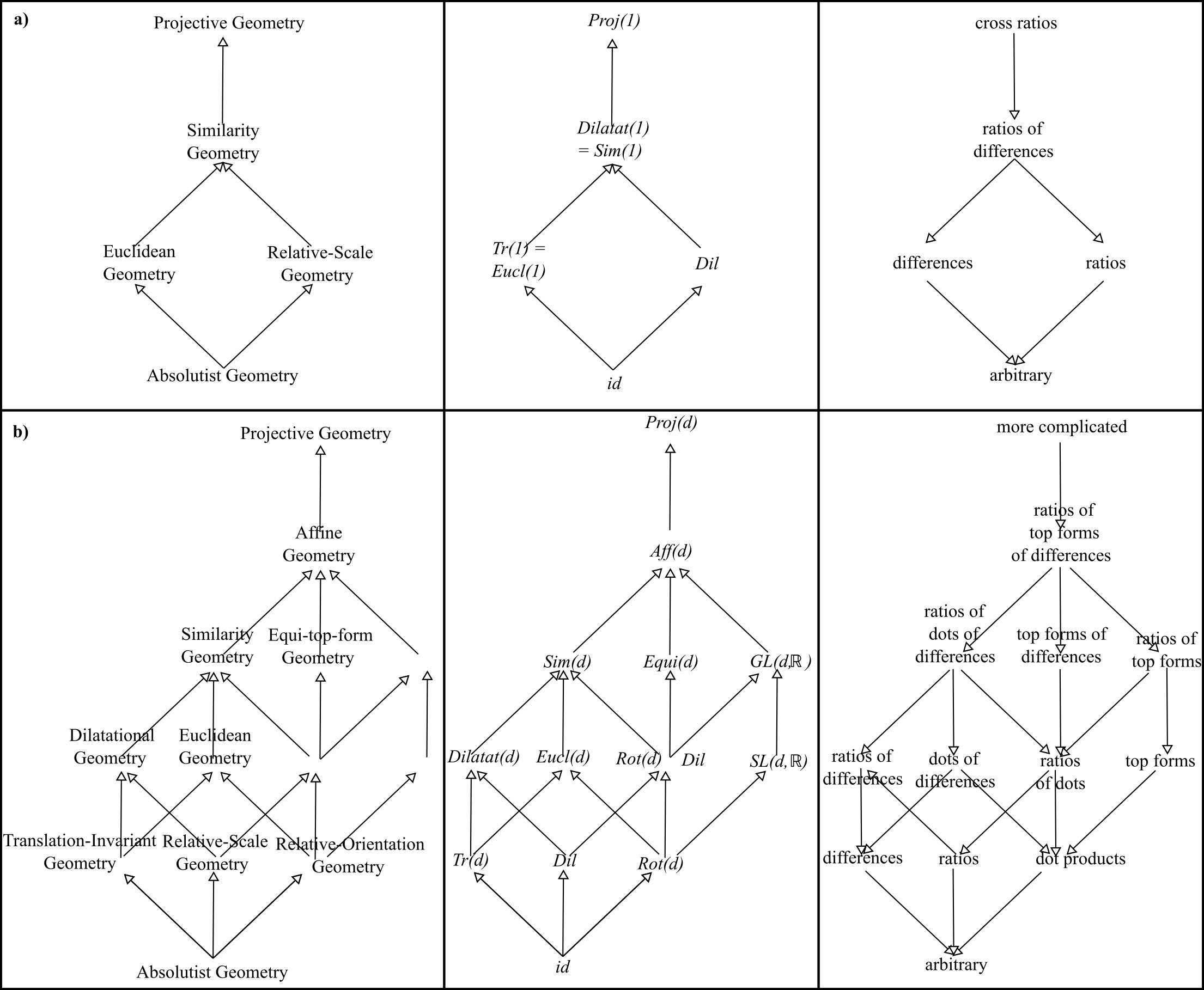
Figure 2: Bounded lattices of notions of geometry, their corresponding automorphism groups, and the corresponding dual lattice of $N$-point invariants. Row a) is for 1-$d$ geometries, and row b) is for higher-$d$ geometries whose automorphism group is a subgroup of the projective group.

References

- [1]
- [2] I. Newton, Philosophiae Naturalis Principia Mathematica (Mathematical Principles of Natural Philosophy) (1686). For an English translation, see e.g. I.B. Cohen and A. Whitman (University of California Press, Berkeley, 1999). In particular, see the Scholium on Time, Place, Space and Motion therein.
- [3] G.W. Leibniz, The Metaphysical Foundations of Mathematics (University of Chicago Press, Chicago 1956), originally dating to 1715; See also The Leibnitz–Clark Correspondence, ed. H.G. Alexander (Manchester 1956), originally dating to 1715 and 1716.
- [4] E. Mach, Die Mechanik in ihrer Entwickelung, Historisch-kritisch dargestellt (J.A. Barth, Leipzig 1883). An English translation is The Science of Mechanics: A Critical and Historical Account of its Development Open Court, La Salle, Ill. 1960).
- [5] O. Veblen and J.W. Young Projective Geometry Vols 1 and 2 (Ginn, Boston 1910).
- [6] D. Hilbert and S. Cohn-Vossen, Geometry and the Imagination (Chelsea, New York 1952; the original, in German, dates to 1932).
- [7] E. Cartan, Collected Works (Gauthier–Villars, Paris 1955).
- [8] R. Arnowitt, S. Deser and C.W. Misner, “The Dynamics of General Relativity", in Gravitation: An Introduction to Current Research ed. L. Witten (Wiley, New York 1962), arXiv:gr-qc/0405109.
- [9] H.W. Guggenheimer, Differential Geometry (McGraw–Hill, New York 1963, reprinted by Dover, New York from 1977 onward).
- [10] P.A.M. Dirac, Lectures on Quantum Mechanics (Yeshiva University, New York 1964).
- [11] J.L. Anderson, “Relativity Principles and the Role of Coordinates in Physics.", in Gravitation and Relativity ed. H-Y. Chiu and W.F. Hoffmann p. 175 (Benjamin, New York 1964); Principles of Relativity Physics (Academic Press, New York 1967).
- [12] H.S.M. Coxeter and S.L. Greitzer, Geometry Revisited (Mathematical Association of America, 1967).
- [13] J.A. Wheeler, in Battelle Rencontres: 1967 Lectures in Mathematics and Physics ed. C. DeWitt and J.A. Wheeler (Benjamin, New York 1968).
- [14] B.S. DeWitt, “Quantum Theory of Gravity. I. The Canonical Theory.", Phys. Rev. 160 1113 (1967).
- [15] S.A. Roach, The Theory of Random Clumping (Methuen, London 1968).
- [16] K. Yano, Integral Formulas in Riemannian Geometry (Dekker, New York 1970).
- [17] S. Smale “Topology and Mechanics. II. The Planar -body Problem, Invent. Math. 11 45 (1970).
- [18] B.S. DeWitt, “Spacetime as a Sheaf of Geodesics in Superspace", in Relativity (Proceedings of the Relativity Conference in the Midwest, held at Cincinnati, Ohio June 2-6, 1969), ed. M. Carmeli, S.I. Fickler and L. Witten (Plenum, New York 1970); A.E. Fischer, “The Theory of Superspace", ibid.
- [19] J.W. York Jr., “Covariant Decompositions of Symmetric Tensors in the Theory of Gravitation", Ann. Inst. Henri Poincaré 21 319 (1974).
- [20] J.B. Barbour and B. Bertotti, “Mach’s Principle and the Structure of Dynamical Theories", Proc. Roy. Soc. Lond. A382 295 (1982).
- [21] D.G. Kendall, “Shape Manifolds, Procrustean Metrics and Complex Projective Spaces", Bull. Lond. Math. Soc. 16 81 (1984).
- [22] T. Iwai, “A Geometric Setting for Internal Motions of the Quantum Three-Body System", J. Math. Phys. 28 1315 (1987).
- [23] H.S.M. Coxeter, Introduction to Geometry (Wiley, New York 1989).
- [24] D.J. Saunders The Geometry of Jet Bundles (C.U.P., Cambridge 1989).
- [25] D.G. Kendall, “A Survey of the Statistical Theory of Shape", Statistical Science 4 87 (1989).
- [26] J.B. Barbour, Absolute or Relative Motion? Vol 1: The Discovery of Dynamics (Cambridge University Press, Cambridge 1989).
- [27] M. Henneaux and C. Teitelboim, Quantization of Gauge Systems (Princeton University Press, Princeton 1992).
- [28] K.V. Kuchař, “Time and Interpretations of Quantum Gravity", in Proceedings of the 4th Canadian Conference on General Relativity and Relativistic Astrophysics ed. G. Kunstatter, D. Vincent and J. Williams (World Scientific, Singapore, 1992), reprinted as Int. J. Mod. Phys. Proc. Suppl. D20 3 (2011).
- [29] C.J. Isham, “Canonical Quantum Gravity and the Problem of Time", in Integrable Systems, Quantum Groups and Quantum Field Theories ed. L.A. Ibort and M.A. Rodríguez (Kluwer, Dordrecht 1993), gr-qc/9210011.
- [30] J.B. Barbour, “The Timelessness of Quantum Gravity. I. The Evidence from the Classical Theory", Class. Quant. Grav. 11 2853 (1994).
- [31] Mach’s principle: From Newton’s Bucket to Quantum Gravity, ed. J.B. Barbour and H. Pfister (Birkhäuser, Boston 1995).
- [32] R.G. Littlejohn and M. Reinsch, “Internal or Shape Coordinates in the -Body Problem", Phys. Rev. A52 2035 (1995).
- [33] C.G.S. Small, The Statistical Theory of Shape (Springer, New York, 1996).
- [34] A.E. Fischer and V. Moncrief, “A Method of Reduction of Einstein’s Equations of Evolution and a Natural Symplectic Structure on the Space of Gravitational Degrees of Freedom", Gen. Rel. Grav. 28, 207 (1996).
- [35] R.G. Littlejohn and M. Reinsch, “Gauge Fields in the Separation of Rotations and Internal Motions in the -Body Problem", Rev. Mod. Phys. 69 213 (1997).
- [36] G. Sparr, “Euclidean and Affine Structure/Motion for Uncalibrated Cameras from Affine Shape and Subsidiary Information", in Proceedings of SMILE Workshop on Structure from Multiple Images, Freiburg (1998).
- [37] D.G. Kendall, D. Barden, T.K. Carne and H. Le, Shape and Shape Theory (Wiley, Chichester 1999).
- [38] K.V. Mardia and P.E. Jupp, Directional Statistics (Wiley, Chichester 2000).
- [39] K.A Mitchell and R.G. Littlejohn, “Kinematic Orbits and the Structure of the Internal Space for Systems of Five or More Bodies", J. Phys. A: Math. Gen. 33 1395 (2000).
- [40] J.B. Barbour, B.Z. Foster and N. ó Murchadha, “Relativity Without Relativity", Class. Quant. Grav. 19 3217 (2002), gr-qc/0012089.
- [41] R. Montgomery, “Infinitely Many Syzygies", Arch. Rat. Mech. Anal. 164 311 (2002).
- [42] H. Stephani, D. Kramer, M.A.H. MacCallum, C.A. Hoenselaers, and E. Herlt, Exact Solutions of Einstein’s Field Equations 2nd Edition (Cambridge University Press, Cambridge 2003).
- [43] V. Patrangenaru and K.V. Mardia, “Affine Shape Analysis and Image Analysis", in Stochastic Geometry, Biological Structure and Images ed. R.G. Aykroyd, K.V. Mardia and M.J. Langdon (Leeds University Press, Leeds 2003).
- [44] J. Stillwell, Mathematics and its History (Springer, 2004).
- [45] J. Stillwell, The Four Pillars of Geometry (Springer, New York 2005).
- [46] V. Ovsienko and S. Tabachnikov, Projective Differential Geometry Old and New (C.U.P., Cambridge 2005).
- [47] E. Anderson, J.B. Barbour, B.Z. Foster, B. Kelleher and N. ó Murchadha, “The Physical Gravitational Degrees of Freedom", Class. Quant. Grav 22 1795 (2005), gr-qc/0407104.
- [48] R. Montgomery, “Fitting Hyperbolic Pants to a 3-Body Problem", Ergod. Th. Dynam. Sys. 25 921 (2005), math/0405014.
- [49] K.V. Mardia and V. Patrangenaru, “Directions and Projective Shapes", Ann. Stat. 33 1666 (2005).
- [50] B. O’Neill, Elementary Differential Geometry (Academic Press, Burlington M.A. 2006).
- [51] D. Giulini, “Some Remarks on the Notions of General Covariance and Background Independence", in An Assessment of Current Paradigms in the Physics of Fundamental Interactions ed. I.O. Stamatescu, Lect. Notes Phys. 721 105 (2007), arXiv:gr-qc/0603087.
- [52] E. Anderson, “Foundations of Relational Particle Dynamics", Class. Quant. Grav. 25 025003 (2008), arXiv:0706.3934.
- [53] D. Giulini, “The Superspace of Geometrodynamics", Gen. Rel. Grav. 41 785 (2009) 785, arXiv:0902.3923.
- [54] D. Groisser, and H.D. Tagare, “On the Topology and Geometry of Spaces of Affine Shapes", Journal of Mathematical Imaging and Vision" 34 222 (2009).
- [55] E. Anderson, “The Problem of Time in Quantum Gravity", in Classical and Quantum Gravity: Theory, Analysis and Applications ed. V.R. Frignanni (Nova, New York 2012), arXiv:1009.2157.
- [56] E. Anderson, “The Problem of Time and Quantum Cosmology in the Relational Particle Mechanics Arena", arXiv:1111.1472.
- [57] A. Bhattacharya and R. Bhattacharya “Nonparametric Statistics on Manifolds with Applications to Shape Spaces" (Cambridge University Press, Cambridge 2012).
- [58] E. Anderson, “Relational Quadrilateralland. I. The Classical Theory", Int. J. Mod. Phys. D23 1450014 (2014), arXiv:1202.4186.
- [59] E. Anderson, “Problem of Time in Quantum Gravity", Annalen der Physik, 524 757 (2012), arXiv:1206.2403.
- [60] J.T. Kent and K.V. Mardia “A Geometric Approach to Projective Space and the Crossratio", Biometrika 99 833 (2012).
- [61] E. Anderson, “Kendall’s Shape Statistics as a Classical Realization of Barbour-type Timeless Records Theory approach to Quantum Gravity", Stud. Hist. Phil. Mod. Phys. 51 1 (2015), arXiv:1307.1923.
- [62] E. Anderson, “Background Independence", arXiv:1310.1524.
- [63] E. Anderson and F. Mercati, “Classical Machian Resolution of the Spacetime Construction Problem", arXiv:1311.6541.
- [64] E. Anderson, “Beables/Observables in Classical and Quantum Gravity", SIGMA 10 092 (2014), arXiv:1312.6073.
- [65] R. Montgomery, “The Three-Body Problem and the Shape Sphere", Amer. Math. Monthly 122 299 (2015), arXiv:1402.084.
- [66] E. Anderson, “Problem of Time and Background Independence: the Individual Facets", arXiv:1409.4117.
- [67] E. Anderson, “Six New Mechanics corresponding to further Shape Theories", Int. J. Mod. Phys. D 25 1650044 (2016), arXiv:1505.00488.
- [68] E. Anderson, “Explicit Partial and Functional Differential Equations for Beables or Observables" arXiv:1505.03551.
- [69] I.L. Dryden, K.V. Mardia, Statistical Shape Analysis: With Applications in R, 2nd Edition (Wiley, Chichester 2016).
- [70] V. Patrangenaru and L. Ellingson “Nonparametric Statistics on Manifolds and their Applications to Object Data Analysis" (Taylor and Francis: Boca Raton, Florida 2016).
- [71] F. Kelma, J.T. Kent and T. Hotz, “On the Topology of Projective Shape Spaces", arXiv:1602.04330.
- [72] The Problem of Time. 2017. Published in Fundam.Theor.Phys. 190 (2017) pp.-
- [73] alias E. Anderson, Problem of Time. Quantum Mechanics versus General Relativity, (Springer International 2017), Found. Phys. 190; free access to its extensive Appendices is at https://link.springer.com/content/pdf/bbm3A978-3-319-58848-32F1.pdf .
- [74] E. Anderson, “The Smallest Shape Spaces. I. Shape Theory Posed, with Example of 3 Points on the Line", arXiv:1711.10054.
- [75] E. Anderson, “The Smallest Shape Spaces. II. 4 Points on a Line Suffices for a Complex Background-Independent Theory of Inhomogeneity", arXiv:1711.10073.
- [76] E. Anderson, “The Smallest Shape Spaces. III. Triangles in the plane and in 3-", arXiv:1711.10115.
- [77] M.P. do Carmo, Differential Geometry of Curves and Surfaces 2nd Edition (Dover, New York 2017).
- [78] E. Anderson, “Two New Perspectives on Heron’s Formula", arXiv:1712.01441.
- [79] E. Anderson, “Maximal Angle Flow on the Shape Sphere of Triangles", arXiv:1712.07966.
- [80] E. Anderson, “Monopoles of Twelve Types in 3-Body Problems", arXiv:1802.03465.
- [81] E. Anderson, “Topological Shape Theory", arXiv:1803.11126.
- [82] E. Anderson, “Background Independence: and absolute spaces differ greatly in Shape-and-Scale Theory", arXiv:1804.10933.
- [83] E. Anderson, “Rubber Relationalism: Smallest Graph-Theoretically Nontrivial Leibniz Spaces", arXiv:1805.03346.
- [84] E. Anderson “Absolute versus Relational Motion Debate: a Modern Global Version", arXiv:1805.09459.
- [85] E. Anderson “-Body Problem: Minimal for Qualitative Nontrivialities", arXiv:1807.08391.
- [86] E. Anderson, “Specific PDEs for Preserved Quantities in Geometry. I. Similarities and Subgroups", arXiv:1809.02045.
- [87] E. Anderson, “Specific PDEs for Preserved Quantities in Geometry. II. Affine Transformations and Subgroups", arXiv:1809.02087.
- [88] E. Anderson, “Specific PDEs for Preserved Quantities in Geometry. III. 1- Projective Transformations and Subgroups", arXiv:1809.02065.
- [89] E. Anderson, “Spaces of Observables from Solving PDEs. I. Translation-Invariant Theory.", arXiv:1809.07738.
- [90] E. Anderson, “Quadrilaterals in Shape Theory. II. Alternative Derivations of Shape Space: Successes and Limitations", arXiv:1810.05282.
- [91] E. Anderson, Geometry from Brackets Consistency, forthcoming October 2018.
- [92] E. Anderson “-Body Problem: Minimal for Qualitative Nontrivialities II: Varying Carrier Space and Group Quotiented Out", forthcoming November 2018.
- [93] E. Anderson, “Nine Pillars of Geometry", forthcoming November 2018.
- [94] E. Anderson, forthcoming.