NestDNN: Resource-Aware Multi-Tenant On-Device Deep Learning for Continuous Mobile Vision

Abstract.

Mobile vision systems such as smartphones, drones, and augmented-reality headsets are revolutionizing our lives. These systems usually run multiple applications concurrently and their available resources at runtime are dynamic due to events such as starting new applications, closing existing applications, and application priority changes. In this paper, we present NestDNN, a framework that takes the dynamics of runtime resources into account to enable resource-aware multi-tenant on-device deep learning for mobile vision systems. NestDNN enables each deep learning model to offer flexible resource-accuracy trade-offs. At runtime, it dynamically selects the optimal resource-accuracy trade-off for each deep learning model to fit the model’s resource demand to the system’s available runtime resources. In doing so, NestDNN efficiently utilizes the limited resources in mobile vision systems to jointly maximize the performance of all the concurrently running applications. Our experiments show that compared to the resource-agnostic status quo approach, NestDNN achieves as much as $4.2\%$ increase in inference accuracy, $2.0\times$ increase in video frame processing rate and $1.7\times$ reduction on energy consumption.

1. Introduction

Mobile systems with onboard video cameras such as smartphones, drones, wearable cameras, and augmented-reality headsets are revolutionizing the way we live, work, and interact with the world. By processing the streaming video inputs, these mobile systems are able to retrieve visual information from the world and are promised to open up a wide range of new applications and services. For example, a drone that can detect vehicles, identify road signs, and track traffic flows will enable mobile traffic surveillance with aerial views that traditional traffic surveillance cameras positioned at fixed locations cannot provide (Puri, 2005). A wearable camera that can recognize everyday objects, identify people, and understand the surrounding environments can be a life-changer for the blind and visually impaired individuals (nvi, 2016).

The key to achieving the full promise of these mobile vision systems is effectively analyzing the streaming video frames. However, processing streaming video frames taken in mobile settings is challenging in two folds. First, the processing usually involves multiple computer vision tasks. This multi-tenant characteristic requires mobile vision systems to concurrently run multiple applications that target different vision tasks (LiKamWa and Zhong, 2015). Second, the context in mobile settings can be frequently changed. This requires mobile vision systems to be able to switch applications to execute new vision tasks encountered in the new context (Han et al., 2016).

In the past few years, deep learning (e.g., Deep Neural Networks (DNNs)) (LeCun et al., 2015) has become the dominant approach in computer vision due to its capability of achieving impressively high accuracies on a variety of important vision tasks (Krizhevsky et al., 2012; Taigman et al., 2014; Zhou et al., 2014). As deep learning chipsets emerge, there is a significant interest in leveraging the on-device computing resources to execute deep learning models on mobile systems without cloud support (goo, 2018; app, 2017; ama, 2018). Compared to the cloud, mobile systems are constrained by limited resources. Unfortunately, deep learning models are known to be resource-demanding (Sze et al., 2017). To enable on-device deep learning, one of the common techniques used by application developers is compressing the deep learning model to reduce its resource demand at a modest loss in accuracy as trade-off (Han et al., 2016; Zhang et al., 2017). Although this technique has gained considerable popularity and has been applied to developing state-of-the-art mobile deep learning systems (Howard et al., 2017; Huynh et al., 2017; Zeng et al., 2017; Lane et al., 2016; Fang et al., 2017), it has a key drawback: since application developers develop their applications independently, the resource-accuracy trade-off of the compressed model is predetermined based on a static resource budget at application development stage and is fixed after the application is deployed. However, the available resources in mobile vision systems at runtime are always dynamic due to events such as starting new applications, closing existing applications, and application priority changes. As such, when the resources available at runtime do not meet the resource demands of the compressed models, resource contention among concurrently running applications occurs, forcing the streaming video to be processed at a much lower frame rate. On the other hand, when extra resources at runtime become available, the compressed models cannot utilize the extra available resources to regain their sacrificed accuracies back.

In this work, we present NestDNN, a framework that takes the dynamics of runtime resources into consideration to enable resource-aware multi-tenant on-device deep learning for mobile vision systems. NestDNN replaces fixed resource-accuracy trade-offs with flexible resource-accuracy trade-offs, and dynamically selects the optimal resource-accuracy trade-off for each deep learning model at runtime to fit the model’s resource demand to the system’s available runtime resources. In doing so, NestDNN is able to efficiently utilize the limited resources in the mobile system to jointly maximize the performance of all the concurrently running applications.

Challenges and our Solutions. The design of NestDNN involves two key technical challenges. (i) The limitation of existing approaches is rooted in the constraint where the trade-off between resource demand and accuracy of a compressed deep learning model is fixed. Therefore, the first challenge lies in designing a scheme that enables a deep learning model to provide flexible resource-accuracy trade-offs. One naive approach is to have all the possible model variants with various resource-accuracy trade-offs installed in the mobile system. However, since these model variants are independent of each other, this approach is not scalable and becomes infeasible when the mobile system concurrently runs multiple deep learning models, with each of which having multiple model variants. (ii) Selecting which resource-accuracy trade-off for each of the concurrently running deep learning models is not trivial. This is because different applications have different goals on inference accuracies and processing latencies. Taking a traffic surveillance drone as an example: an application that counts vehicles to detect traffic jams does not need high accuracy but requires low latency; an application that reads license plates needs high plate reading accuracy but does not require real-time response (Zhang et al., 2017).

To address the first challenge, NestDNN employs a novel model pruning and recovery scheme which transforms a deep learning model into a single compact multi-capacity model. The multi-capacity model is comprised of a set of descendent models, each of which offers a unique resource-accuracy trade-off. Unlike traditional model variants that are independent of each other, the descendent model with smaller capacity (i.e., resource demand) shares its model parameters with the descendent model with larger capacity, making itself nested inside the descendent model with larger capacity without taking extra memory space. In doing so, the multi-capacity model is able to provide various resource-accuracy trade-offs with a compact memory footprint.

To address the second challenge, NestDNN encodes the inference accuracy and processing latency of each descendent model of each concurrently running application into a cost function. Given all the cost functions, NestDNN employs a resource-aware runtime scheduler which selects the optimal resource-accuracy trade-off for each deep learning model and determines the optimal amount of runtime resources to allocate to each model to jointly maximize the overall inference accuracy and minimize the overall processing latency of all the concurrently running applications.

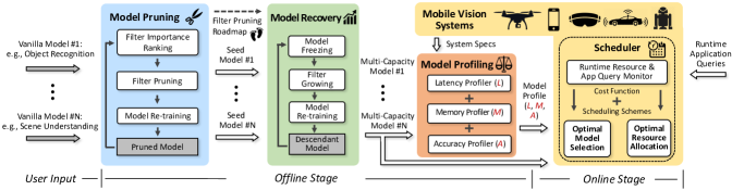
Figure 1. NestDNN architecture.

Summary of Experimental Results. We have conducted a rich set of experiments to evaluate the performance of NestDNN. To evaluate the performance of the multi-capacity model, we evaluated it on six mobile vision applications that target some of the most important tasks for mobile vision systems. These applications are developed based on two widely used deep learning models – VGG Net (Simonyan and Zisserman, 2014) and ResNet (He et al., 2016) – and six datasets that are commonly used in computer vision community. To evaluate the performance of the resource-aware runtime scheduler, we incorporated two widely used scheduling schemes and implemented NestDNN and the six mobile vision applications on three smartphones. We also implemented the status quo approach which uses fixed resource-accuracy trade-off and is thus resource-agnostic. To compare the performance between our resource-aware approach with the resource-agnostic status quo approach, we have designed a benchmark that emulates runtime application queries in diverse scenarios. Our results show that:

• The multi-capacity model is able to provide flexible and optimized resource-accuracy trade-offs nested in a single model. With parameter sharing, it significantly reduces model memory footprint and model switching overhead.

• The resource-aware runtime scheduler outperforms the resource-agnostic counterpart on both scheduling schemes, achieving as much as $4.2\%$ increase in inference accuracy, $2.0\times$ increase in video frame processing rate and $1.7\times$ reduction on energy consumption.

Summary of Contributions. To the best of our knowledge, NestDNN represents the first framework that enables resource-aware multi-tenant on-device deep learning for mobile vision systems. It contributes novel techniques that address the limitations in existing approaches as well as the unique challenges in continuous mobile vision. We believe our work represents a significant step towards turning the envisioned continuous mobile vision into reality (Bahl et al., 2012; LiKamWa and Zhong, 2015; Naderiparizi et al., 2017).

2. NestDNN Overview

Figure 1 illustrates the architecture of NestDNN, which is split into an offline stage and an online stage.

The offline stage consists of three phases: model pruning (§3.1), model recovery (§3.2), and model profiling.

In the model pruning phase, NestDNN employs a state-of-the-art Triplet Response Residual (TRR) approach to rank the filters in a given deep learning model (i.e., vanilla model) based on their importance and prune the filters iteratively. In each iteration, less important filters are pruned, and the pruned model is retrained to compensate the accuracy degradation (if there is any) caused by filter pruning. The iteration ends when the pruned model could not meet the minimum accuracy goal set by the user. The smallest pruned model is called seed model. As a result, a filter pruning roadmap is created where each footprint on the roadmap is a pruned model with its filter pruning record.

In the model recovery phase, NestDNN employs a novel model freezing and filter growing (i.e., freeze-&-grow) approach to generate the multi-capacity model in an iterative manner. Model recovery uses the seed model as the starting point. In each iteration, model freezing is first applied to freeze the parameters of all the model’s filters. By following the filter pruning roadmap in the reverse order, filter growing is then applied to add the pruned filters back. As such, a descendant model with a larger capacity is generated and its accuracy is regained via retraining. By repeating the iteration, a new descendant model is grown upon the previous one. Thus, the final descendant model has the capacities of all the previous ones and is thus named multi-capacity model.

Terminology	Explanation
Vanilla Model	Off-the-shelf deep learning model (e.g., ResNet) trained on a given dataset (e.g., ImageNet).
Pruned Model	Intermediate result obtained in model pruning stage.
Seed Model	The smallest pruned model generated in model pruning which meets the minimum accuracy goal set by the user. It is also the starting point of model recovery stage.
Descendant Model	A model grown upon the seed model in model recovery stage. It has a unique resource-accuracy trade-off.
Multi-Capacity Model	The final descendant model that has the capacities of all the previously generated descendant models.

Table 1. Terminologies involved in NestDNN.

In the model profiling phase, given the specs of a mobile vision system, a profile is generated for each multi-capacity model including the inference accuracy, memory footprint, and processing latency of each of its descendent models.

Finally, in the online stage, the resource-aware runtime scheduler (§3.3) continuously monitors events that change runtime resources. Once such event is detected, the scheduler checks up the profiles of all the concurrently running applications, selects the optimal descendant model for each application, and allocates the optimal amount of runtime resources to each selected descendant model to jointly maximize the overall inference accuracy and minimize the overall processing latency of all those applications.

For clarification purpose, Table 1 summarizes the terminologies defined in this work and their brief explanations.

3. Design of NestDNN

3.1. Filter based Model Pruning

3.1.1. Background on CNN Architecture

Before delving deep into filter pruning, it is important to understand the architecture of a convolutional neural network (CNN). In general, a CNN consists of four types of layers: convolutional layers, activation layers, pooling layers, and fully-connected layers. Due to the computational intensity of convolution operations, convolutional layers are the most computational intensive layers among the four types of layers. Specifically, each convolutional layer is composed of a set of 3D filters, which plays the role of “feature extractors”. By convolving an image with these 3D filters, it generates a set of features organized in the form of feature maps, which are further sent to the following convolutional layers for further feature extraction.

3.1.2. Benefits of Filter Pruning

Figure 2 illustrates the details of filter pruning. Let $\Theta_{j-1}\in\mathbb{R}^{w_{j-1}\times h_{j-1}\times m_{j-1}}$ denote the input feature maps of the $j$th convolutional layer $conv_{j}$ of a CNN, where $w_{j-1}$ and $h_{j-1}$ are the width and height of each of the input feature maps; and $m_{j-1}$ is the total number of the input feature maps. The convolutional layer $conv_{j}$ consists of $m_{j}$ 3D filters with size $k\times k\times m_{j-1}$ ($k\times k$ is the 2D kernel). It applies these filters onto the input feature maps $\Theta_{j-1}$ to generate the output feature maps $\Theta_{j}\in\mathbb{R}^{w_{j}\times h_{j}\times m_{j}}$, where one 3D filter generates one output feature map. This process involves a total of $m_{j}k^{2}m_{j-1}w_{j}h_{j}$ floating point operations (i.e., FLOPs).

Since one 3D filter generates one output feature map, pruning one 3D filter in $conv_{j}$ (marked in green in $conv_{j}$) results in removing one output feature map in $\Theta_{j}$ (marked in green in $\Theta_{j}$), which leads to $k^{2}m_{j-1}$ parameter and $k^{2}m_{j-1}w_{j}h_{j}$ FLOPs reduction. Subsequently, $m_{j+1}$ 2D kernels applied onto that removed output feature map in the convolutional layer $conv_{j+1}$ (marked in green in $conv_{j+1}$) are also removed. This leads to an additional $k^{2}m_{j+1}$ parameter and $k^{2}m_{j+1}w_{j+1}h_{j+1}$ FLOPs reduction. Therefore, by pruning filters, both model size (i.e., model parameters) and computational cost (i.e., FLOPs) are reduced (Li et al., 2016).

3.1.3. Filter Importance Ranking

The key to filter pruning is identifying less important filters. By pruning those filters, the size and computational cost of a CNN model can be effectively reduced.

To this end, we propose a filter importance ranking approach named Triplet Response Residual (TRR) to measure the importance of filters and rank filters based on their relative importance. Our TRR approach is inspired by one key intuition: since a filter plays the role of “feature extractor”, a filter is important if it is able to extract feature maps that are useful to differentiate images belonging to different classes. In other words, a filter is important if the feature maps it extracts from images belonging to the same class are more similar than the ones extracted from images belonging to different classes.

Let {$anc$, $pos$, $neg$} denote a triplet that consists of an anchor image ($anc$), a positive image ($pos$), and a negative image ($neg$) where the anchor image and the positive image are from the same class, while the negative image is from a different class. By following the key intuition, TRR of filter $i$ is defined as:

(1) $$TRR_{i}=\sum(\lVert\mathcal{F}_{i}(anc)-\mathcal{F}_{i}(neg)\rVert^{2}_{2}-\lVert\mathcal{F}_{i}(anc)-\mathcal{F}_{i}(pos)\rVert^{2}_{2})$$

where $\mathcal{F}(\cdot)$ denotes the generated feature map. Essentially, TRR calculates the $\mathcal{L}2$ distances of feature maps between ($anc$, $neg$) and between ($anc$, $pos$), and measures the residual between the two distances. By summing up the residuals of all the triplets from the training dataset, the value of TRR of a particular filter reflects its capability of differentiating images belonging to different classes, acting as a measure of importance of the filter within the CNN model.

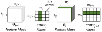
Figure 2. Illustration of filter pruning (Li et al., 2016). By pruning filters, both model size and computational cost are reduced.

3.1.4. Performance of Filter Importance Ranking

Figure 3(a) illustrates the filter importance profiling performance of our TRR approach on VGG-16 (Simonyan and Zisserman, 2014) trained on the CIFAR-10 dataset (Krizhevsky and Hinton, 2009). The vanilla VGG-16 model contains 13 convolutional layers. Each of the 13 curves in the figure depicts the top-1 accuracies when filters of one particular convolutional layer are pruned while the other convolutional layers remain unmodified. Each marker on the curve corresponds to the top-1 accuracy when a particular percentage of filters is pruned. As an example, the topmost curve (blue dotted line with blue triangle markers) shows the accuracies are 89.75%, 89.72% and 87.40% when 0% (i.e., vanilla model), 50% and 90% of the filters in the 13th convolutional layer $conv_{13}$ are pruned, respectively.

We have two key observations from the filter importance profiling result. First, we observe that our TRR approach is able to effectively identify redundant filters within each convolutional layer. In particular, the accuracy remains the same when 59.96% of the filters in $conv_{13}$ are pruned. This indicates that these pruned filters, identified by TRR, are redundant. By pruning these redundant filters, the vanilla VGG-16 model can be effectively compressed without any accuracy degradation. Second, we observe that our TRR approach is able to effectively identify convolutional layers that are more sensitive to filter pruning. This is reflected by the differences in accuracy drops when the same percentage of filters are pruned at different convolutional layers. This sensitivity difference across convolutional layers has been taken into account in the iterative filter pruning process.

To demonstrate the superiority of our TRR approach, we have compared it with the state-of-the-art filter pruning approach. The state-of-the-art filter pruning approach uses $\mathcal{L}1$-norm of a filter to measure its importance (Li et al., 2016). Figure 3(b) illustrates the filter importance profiling performance of $\mathcal{L}1$-norm on the same vanilla VGG-16 model trained on the CIFAR-10 dataset. By comparing Figure 3(a) to Figure 3(b), we observe that TRR achieves better accuracy than $\mathcal{L}1$-norm at almost every pruned filter percentage across all 13 curves. As a concrete example, TRR achieves an accuracy of 89.72% and 87.40% when 50% and 90% of the filters at $conv_{13}$ are pruned respectively, while $\mathcal{L}1$-norm only achieves an accuracy of 75.45% and 42.65% correspondingly. This result indicates that the filters pruned by TRR have much less impact on accuracy than the ones pruned by $\mathcal{L}1$-norm, demonstrating that TRR outperforms $\mathcal{L}1$-norm at identifying less important filters.

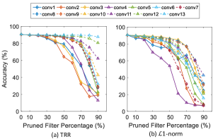
Figure 3. Filter importance profiling performance of (a) TRR and (b) $\mathcal{L}1$-norm on VGG-16 trained on CIFAR-10.

3.1.5. Filter Pruning Roadmap

By following the filter importance ranking provided by TRR, we iteratively prune the filters in a CNN model. During each iteration, less important filters across convolutional layers are pruned, and the pruned model is retrained to compensate the accuracy degradation (if there is any) caused by filter pruning. The iteration ends when the pruned model could not meet the minimum accuracy goal set by the user. As a result, a filter pruning roadmap is created where each footprint on the roadmap is a pruned model with its filter pruning record. The smallest pruned model on the roadmap is called seed model. This filter pruning roadmap is used to guide the model recovery process described below.

3.2. Freeze-&-Grow based Model Recovery

3.2.1. Motivation and Key Idea

The filter pruning process generates a series of pruned models, each of which acting as a model variant of the vanilla model with a unique resource-accuracy trade-off. However, due to the retraining step within each pruning iteration, these pruned models have different model parameters, and thus are independent of each other. Therefore, although these pruned models provide different resource-accuracy trade-offs, keeping all of them locally in resource-limited mobile systems is practically infeasible.

To address this problem, we propose to generate a single multi-capacity model that acts equivalently as the series of pruned models to provide various resource-accuracy trade-offs but has a model size that is much smaller than the accumulated model size of all the pruned models. This is achieved by an innovative model freezing and filter growing (i.e., freeze-&-grow) approach.

In the remainder of this section, we describe the details of the freeze-&-grow approach and how the multi-capacity model is iteratively generated.

3.2.2. Model Freezing and Filter Growing

The generation of the multi-capacity model starts from the seed model derived from the filter pruning process. By following the filter pruning roadmap and the freeze-&-grow approach, the multi-capacity model is iteratively created.

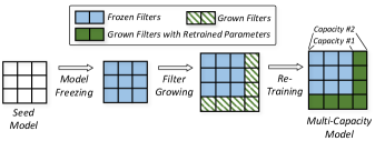
Figure 4. Illustration of model freezing and filter growing.

Figure 4 illustrates the details of model freezing and filter growing during the first iteration. For illustration purpose, only one convolutional layer is depicted. As shown, given the seed model, we first apply model freezing to freeze the parameters of all its filters (marked as blue squares). Next, since each footprint on the roadmap has its filter pruning record, we follow the filter pruning roadmap in the reverse order and apply filter growing to add the pruned filters back (marked as green stripe squares). With the added filters, the capacity of this descendant model is increased. Lastly, we retrain this descendant model to regain accuracy. It is important to note that during retraining, since the seed model is frozen, its parameters are not changed; only the parameters of the added filters are changed (marked as green solid squares to indicate the parameters are changed). As such, we have generated a single model that not only has the capacity of the seed model but also has the capacity of the descendant model. Moreover, the seed model shares all its model parameters with the descendant model, making itself nested inside the descendant model without taking extra memory space.

By repeating the iteration, a new descendant model is grown upon the previous one. As such, the final descendant model has the capacities of all the previous descendant models and is thus named multi-capacity model.

3.2.3. Superiority of Multi-Capacity Model

The generated multi-capacity model has three advantages.

One Compact Model with Multiple Capabilities. The generated multi-capacity model is able to provide multiple capacities nested in a single model. This eliminates the need of installing potentially a large number of independent model variants with different capacities. Moreover, by sharing parameters among descendant models, the multi-capacity model is able to save a large amount of memory space to significantly reduce its memory footprint.

Optimized Resource-Accuracy Trade-offs. Each capacity provided by the multi-capacity model has a unique optimized resource-accuracy trade-off. Our TRR approach is able to provide state-of-the-art performance at identifying and pruning less important filters. As a result, the multi-capacity model delivers state-of-the-art inference accuracy under a given resource budget.

Efficient Model Switching. Because of parameter sharing, the multi-capacity model is able to switch models with little overhead. Switching independent deep learning models causes significant overhead. This is because it requires to page in and page out the entire deep learning models. Multi-capacity model alleviates this problem in an elegant manner by only requiring to page in and page out a very small portion of deep learning models.

Figure 5 illustrates the details of model switching of multi-capacity model. For illustration purpose, only one convolutional layer is depicted. As shown, since each descendant model is grown upon its previous descendant models, when the multi-capacity model is switching to a descendant model with larger capability (i.e., model upgrade), it incurs zero page-out overhead, and only needs to page in the extra filters included in the descendant model with larger capability (marked as green squares). When the multi-capacity model is switching to a descendant model with smaller capability (i.e., model downgrade), it incurs zero page-in overhead, and only needs to page out the filters that the descendant model with smaller capability does not have (marked as gray squares). As a result, the multi-capacity model significantly reduces the overhead of model page in and page out, making model switching extremely efficient.

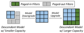
Figure 5. Illustration of model switching (model upgrade vs. model downgrade) of multi-capacity model.

3.3. Resource-Aware Scheduler

3.3.1. Motivation and Key Idea

The creation of the multi-capacity model enables NestDNN to jointly maximize the performance of vision applications that are concurrently running on a mobile vision system. This possibility comes from two key insights. First, while a certain amount of runtime resources can be traded for an accuracy gain in some application, the same amount of runtime resources may be traded for a larger accuracy gain in some other application. Second, for applications that do not need real-time response and thus can tolerate a relatively large processing latency, we can reallocate some runtime resources from those latency-tolerant applications to other applications that need more runtime resources to meet their real-time goals. NestDNN exploits these two key insights by encoding the inference accuracy and processing latency into a cost function for each vision application, which serves as the foundation for resource-aware scheduling.

3.3.2. Cost Function

Let $V$ denote the set of vision applications that are concurrently running on a mobile vision system, and let $A_{min}(v)$ and $L_{max}(v)$ denote the minimum inference accuracy and the maximum processing latency goals set by the user for application $v\in V$. Additionally, let $M_{v}$ denote the multi-capacity model generated for application $v$, and let $m_{v}$ denote a descendant model $m_{v}\in M_{v}$. The cost function of the descendant model $m_{v}$ for application $v$ is defined as follows:

(2) $$C(m_{v},u_{v},v)=(A_{min}(v)-A(m_{v}))+$$

$$\alpha\cdot\max(0,\frac{L(m_{v})}{u_{v}}-L_{max}(v))$$

where $A(m_{v})$ is the inference accuracy of $m_{v}$, $u_{v}\in(0,1]$ is the computing resource percentage allocated to $v$, and $L(m_{v})$ is the processing latency of $m_{v}$ when 100% computing resources are allocated to $v$.

Essentially, the first term in the cost function promotes selecting the descendant model $m_{v}$ whose inference accuracy is as high as possible. The second term in the cost function penalizes selecting the descendant model $m_{v}$ that has a processing latency higher than the maximum processing latency goal. Since the video input is streamed at a dedicated frame rate, there is no reward for achieving a processing latency lower than $L_{max}(v)$. $\alpha\in[0,1]$ is a knob set by the user to determine the latency-accuracy trade-off preference. A large $\alpha$ weights more on the penalty for latency while a small $\alpha$ favors higher accuracy.

3.3.3. Scheduling Schemes

Given the cost function of each descendant model of each concurrently running application, the resource-aware scheduler incorporates two widely used scheduling schemes to jointly maximize the performance of concurrent vision applications for two different optimization objectives.

MinTotalCost. The MinTotalCost (i.e., minimize the total cost) scheduling scheme aims to minimize the total cost of all concurrent applications. This optimization problem can be formulated as follows:

(3) $$\min_{u_{v},m_{v}\in M_{v}}\sum\limits_{v\in V}C(m_{v},u_{v},v)$$

$$s.t.\quad\sum\limits_{v\in V}S(m_{v})\leq S_{max},\quad\sum\limits_{v\in V}u_{v}\leq 1\vspace{2mm}$$

where $S(m_{v})$ denotes the runtime memory footprint of the descendant model $m_{v}$. The total memory footprint of all the concurrent applications cannot exceed the maximum memory space of the mobile vision system denoted as $S_{max}$.

Under the MinTotalCost scheduling scheme, the resource-aware scheduler favors applications with lower costs and thus is optimized to allocate more runtime resources to them.

MinMaxCost. The MinMaxCost (i.e., minimize the maximum cost) scheduling scheme aims to minimize the cost of the application that has the highest cost. This optimization problem can be formulated as follows:

(4) $$\min_{u_{v},m_{v}\in M_{v}}k$$

$$s.t.\quad\forall v:C(m_{v},u_{v},v)\leq k,\vspace{2mm}$$

$$\sum\limits_{v\in V}S(m_{v})\leq S_{max},\quad\sum\limits_{v\in V}u_{v}\leq 1\vspace{2mm}$$

where the cost of any of the concurrently running applications must be smaller than $k$ where $k$ is minimized.

Under the MinMaxCost scheduling scheme, the resource-aware scheduler is optimized to fairly allocate runtime resources to all the concurrent applications to balance their performance.

3.3.4. Cached Greedy Heuristic Approximation

Solving the nonlinear optimization problems involved in MinTotalCost and MinMaxCost scheduling schemes is computationally hard. To enable real-time online scheduling in mobile systems, we utilize a greedy heuristic inspired by (Zhang et al., 2017) to obtain approximate solutions.

Specifically, we define a minimum indivisible runtime resource unit $\Delta u$ (e.g., $1\%$ of the total computing resources in a mobile vision system) and start allocating the computing resources from scratch. For MinTotalCost, we allocate $\Delta u$ to the descendent model $m_{v}$ of application $v$ such that $C(m_{v},\Delta u,v)$ has the smallest cost increase among other concurrent applications. For MinMaxCost, we select application $v$ with the highest cost $C(m_{v},u_{v},v)$, and allocate $\Delta u$ to $v$ and choose the optimal descendent model $m_{v}=\arg\min_{m_{v}}C(m_{v},u_{v},v)$ for $v$. For both MinTotalCost and MinMaxCost, the runtime resources are iteratively allocated until exhausted.

The runtime of executing the greedy heuristic can be further shortened via the caching technique. This is particularly attractive to mobile systems with very limited resources. Specifically, when allocating the computing resources, instead of starting from scratch, we start from the point where a certain amount of computing resources has already been allocated. For example, we can cache the unfinished running scheme where $70\%$ of the computing resources have been allocated during optimization. In the next optimization iteration, we directly start from the unfinished running scheme and allocate the remaining $30\%$ computing resources, thus saving $70\%$ of the optimization time. To prevent from falling into a local minimum over time, a complete execution of the greedy heuristic is performed periodically to enforce the cached solution to be close to the optimal one.

4. Evaluation

4.1. Datasets, DNNs and Applications

4.1.1. Datasets

To evaluate the generalization capability of NestDNN on different vision tasks, we select two types of tasks that are among the most important tasks for mobile vision systems.

Generic-Category Object Recognition. This type of vision tasks aims to recognize the generic category of an object (e.g., a road sign, a person, or an indoor place). Without loss of generality, we select 3 commonly used computer vision datasets, each containing a small, a medium, and a large number of object categories respectively, representing an easy, a moderate, and a difficult vision task correspondingly.

• CIFAR-10 (Krizhevsky and Hinton, 2009). This dataset contains 50K training images and 10K testing images belonging to 10 generic categories of objects.

• ImageNet-50 (Russakovsky et al., 2015). This dataset is a subset of the ILSVRC ImageNet. It contains 63K training images and 2K testing images belonging to top 50 most popular object categories based on the popularity ranking provided by the official ImageNet website.

• ImageNet-100 (Russakovsky et al., 2015). Similar to ImageNet-50, this dataset is a subset of the ILSVRC ImageNet. It contains 121K training images and 5K testing images belonging to top 100 most popular object categories based on the popularity ranking provided by the official ImageNet website.

Class-Specific Object Recognition. This type of vision tasks aims to recognize the specific class of an object within a generic category (e.g., a stop sign, a female person, or a kitchen). Without loss of generality, we select 3 object categories: 1) road signs, 2) people, and 3) places, which are commonly seen in mobile settings.

• GTSRB (Stallkamp et al., 2012). This dataset contains over 50K images belonging to 43 classes of road signs such as speed limit signs and stop signs.

• Adience-Gender (Levi and Hassner, 2015). This dataset contains over 14K images of human faces of two genders.

• Places-32 (Zhou et al., 2017). This dataset is a subset of the Places365-Standard dataset. Places365-Standard contains 1.8 million images of 365 scene classes belonging to 16 higher-level categories. We select two representative scene classes (e.g., parking lot and kitchen) from each of the 16 higher-level categories and obtain a 32-class dataset that includes over 158K images.

4.1.2. DNN Models

To evaluate the generalization capability of NestDNN on different DNN models, we select two representative DNN models: 1) VGG-16 and 2) ResNet-50. VGG-16 (Simonyan and Zisserman, 2014) is considered as one of the most straightforward DNN models to implement, and thus gains considerable popularity in both academia and industry. ResNet-50 (He et al., 2016) is considered as one of the top-performing DNN models in computer vision due to its superior recognition accuracy.

4.1.3. Mobile Vision Applications

Without loss of generality, we randomly assign CIFAR-10, GTSRB and Adience-Gender to VGG-16; and assign ImageNet-50, ImageNet-100 and Places-32 to ResNet-50 to create six mobile vision applications labeled as VC (i.e., VGG-16 trained on the CIFAR-10 dataset), RI-50, RI-100, VS, VG, and RP, respectively. We train and test all the vanilla DNN models and all the descendant models generated by NestDNN by strictly following the protocol provided by each of the six datasets described above.

The datasets, DNN models, and mobile vision applications are summarized in Table 2.

Type	Dataset	DNN Model	Mobile Vision Application
Generic Category	CIFAR-10	VGG-16	VC
	ImageNet-50	ResNet-50	RI-50
	ImageNet-100	ResNet-50	RI-100
Class Specific	GTSRB	VGG-16	VS
	Adience-Gender	VGG-16	VG
	Places-32	ResNet-50	RP

Table 2. Summary of datasets, DNN models, and mobile vision applications used in this work.

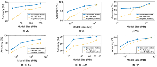
Figure 6. Top-1 accuracy vs. model size comparison between descendent models and baseline models.

4.2. Performance of Multi-Capacity Model

In this section, we evaluate the performance of multi-capacity model to demonstrate its superiority listed in §3.2.3.

4.2.1. Experimental Setup

Selection of Descendant Models. Without loss of generality, for each mobile vision application, we generate a multi-capacity model that contains five descendant models. These descendant models are designed to have diverse resource-accuracy trade-offs. We select these descendant models with the purpose to demonstrate that our multi-capacity model enables applications to run even when available resources are very limited. It should be noted that a multi-capacity model is neither limited to one particular set of resource-accuracy trade-offs nor limited to one particular number of descendant models. NestDNN provides the flexibility to design a multi-capacity model based on users’ preferences.

Baseline. To make a fair comparison, we use the same architecture of descendant models for baseline models such that their model sizes and computational costs are identical. In addition, we pre-trained baseline models on ImageNet dataset and then fine-tuned them on each of the six datasets. Pre-training is an effective way to boost accuracy, and thus is adopted as a routine in machine learning community (Oquab et al., 2014; Huh et al., 2016). We also trained baseline models without pre-training, and observed that baseline models with pre-training consistently outperform those without pre-training. Therefore, we only report accuracies of baseline models with pre-training.

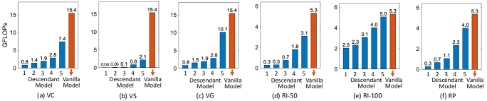
Figure 7. Computational cost comparison between descendant models and vanilla models.

4.2.2. Optimized Resource-Accuracy Trade-offs

Figure 6 illustrates the comparison between descendent models and baseline models across six mobile vision applications. For each application, we show the top-1 accuracies of both descendant models and baseline models as a function of model size. For better illustration purpose, the horizontal axis is plotted using the logarithmic scale.

We have two key observations from the result. First, we observe that descendant models consistently achieve higher accuracies than baseline models at every model size across all the six applications. On average, descendant models achieve 4.98% higher accuracy than baseline models. This indicates that our descendant model at each capacity is able to deliver state-of-the-art inference accuracy under a given memory budget. Second, we observe that smaller descendant models outperform baseline models more than larger descendant models. On average, the two smallest descendant models achieve 6.68% higher accuracy while the two largest descendant models achieve 3.72% higher accuracy compared to their corresponding baseline models. This is because our TRR approach is able to preserve important filters while pruning less important ones. Despite having a small capacity, a small descendant model benefits from these important filters while the corresponding baseline model does not.

Figure 7 shows the computational costs of five descendant models and the corresponding vanilla models of the six applications in GFLOPs (i.e., GigaFLOPs). As shown, all descendant models have less GFLOPs than the corresponding vanilla models. This result indicates that our filter pruning approach is able to effectively reduce the computational costs across six applications, demonstrating the generalization of our filter pruning approach on different deep learning models trained on different datasets.

4.2.3. Reduction on Memory Footprint

Another key feature of multi-capacity model is sharing parameters among its descendant models. To quantify the benefit of parameter sharing on reducing memory footprint, we compare the model size of multi-capacity model with the accumulated model size of the five descendant models as if they were independent. This mimics traditional model variants that are used in existing mobile deep learning systems.

Table 3 lists the comparison results across the six mobile vision applications. Obviously, the model size of the multi-capacity model is smaller than the corresponding accumulated model size for each application. Moreover, deep learning model with larger model size benefits more from parameter sharing. For example, VC has the largest model size across the six applications. With parameter sharing, it achieves a reduced memory footprint of 241.5 MB. Finally, if we consider running all the six applications concurrently, the multi-capacity model achieves a reduced memory footprint of 587.4 MB, demonstrating the enormous benefit of multi-capacity model on memory footprint reduction.

Application	Multi-Capacity Model Size (MB)	Accumulated Model Size (MB)	Reduced Memory Footprint (MB)
VC	196.0	437.5	241.5
VS	12.9	19.8	6.9
VG	123.8	256.0	132.2
RI-50	42.4	58.1	15.7
RI-100	87.1	243.5	156.4
RP	62.4	97.1	34.7
All Included	524.6	1112.0	587.4

Table 3. Benefit of multi-capacity model on memory footprint reduction.

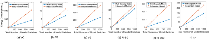
Figure 8. Model switching energy consumption comparison between multi-capacity models and independent models. The energy consumption is measured on a Samsung Galaxy S8 smartphone.

4.2.4. Reduction on Model Switching Overhead

Another benefit of parameter sharing is reducing the overhead of model switching when the set of concurrent applications changes. To quantify this benefit, we consider all the possible model switching cases among all the five descendant models of each multi-capacity model, and calculate the average page-in and page-out overhead for model upgrade and model downgrade, respectively. We compare it with the case where descendant models are treated as if they were independent, which again mimics traditional model variants.

Table 4 lists the comparison results of all six mobile vision applications for model upgrade in terms of memory usage. As expected, the average page-in and page-out memory usage of independent models during model switching is larger than multi-capacity models for every application. This is because during model switching, independent models need to page in and page out the entire models while multi-capacity models only need to page in a very small portion of the models. It should be noted that the page-out overhead of multi-capacity model during model upgrade is zero. This is because the descendant model with smaller capability is part of the descendant model with larger capability, and thus it does not need to be paged out.

Table 5 lists the comparison results of all six applications for model downgrade. Similar results are observed. The only difference is that during model downgrade, the page-in overhead of multi-capacity model is zero.

Besides memory usage, we also quantify the benefit on reducing the overhead of model switching in terms of energy consumption. Specifically, we measured energy consumed by randomly switching models for 250, 500, 750, and 1,000 times using descendant models and independent models, respectively. Figure 8 shows the comparison results across all six mobile vision applications. As expected, energy consumed by switching multi-capacity model is lower than switching independent models for every application. This benefit becomes more prominent when the model size is large. For example, the size of the largest descendant model of VC and VS is 196.0 MB and 12.9 MB, respectively. The corresponding energy consumption reduction for every 1,000 model switches is 602.1 J and 4.0 J, respectively.

Taken together, the generated multi-capacity model is able to significantly reduce the overhead of model switching in terms of both memory usage and energy consumption. The benefit becomes more prominent when model switching frequency increases. This is particularly important for memory and battery constrained mobile systems.

Application	Multi-Capacity Model Upgrade Overhead (MB)		Independent Models Upgrade Overhead (MB)
	Page-In	Page-Out	Page-In	Page-Out
VC	81.4	0	128.2	46.8
VS	1.3	0	1.7	0.3
VG	50.0	0	76.2	26.2
RI-50	19.2	0	21.2	2.0
RI-100	38.3	0	67.9	29.5
RP	26.4	0	34.9	4.6

Table 4. Benefit of multi-capacity model on model switching (model upgrade) in terms of memory usage.

Application	Multi-Capacity Model Downgrade Overhead (MB)		Independent Models Downgrade Overhead (MB)
	Page-In	Page-Out	Page-In	Page-Out
VC	0	81.4	46.8	128.2
VS	0	1.3	0.3	1.7
VG	0	50.0	26.2	76.2
RI-50	0	19.2	2.0	21.2
RI-100	0	38.3	29.5	67.9
RP	0	26.4	4.6	34.9

Table 5. Benefit of multi-capacity model on model switching (model downgrade) in terms of memory usage.

4.3. Performance of Resource-Aware Scheduler

4.3.1. Experimental Setup

Deployment Platforms. We implemented NestDNN and the six mobile vision applications on three smartphones: Samsung Galaxy S8, Samsung Galaxy S7, and LG Nexus 5, all running Android OS 7.0. We used Monsoon power monitor (mon, 2016) to measure the power consumption. We have achieved consistent results across all three smartphones. Here we only report the best results obtained from Samsung Galaxy S8.

Baseline. We used the status quo approach (i.e., resource-agnostic) which uses fixed resource-accuracy trade-off as the baseline. It uses the model located at the “knee” of every yellow curve in Figure 6. This is the one that achieves the best resource-accuracy trade-off among all the model variants.

Benchmark Design. To compare the performance between our resource-aware approach and the resource-agnostic status quo approach, we have designed a benchmark that emulates runtime application queries in diverse scenarios. Specifically, our benchmark creates a new application or kills a running application with certain probabilities at every second. The number of concurrently running applications is from 2 to 6. The maximum available memory to run concurrent applications is set to $400$ MB. Each simulation generated by our benchmark lasts for $60$ seconds. We repeat the simulation 100 times and report the average runtime performance.

Figure 9 shows the profile of all accumulated simulation traces generated by our benchmark. Figure 9(a) shows the time distribution of different numbers of concurrent applications. As shown, the percentage of time when two, three, four, five and six applications running concurrently is 9.8%, 12.7%, 18.6%, 24.5% and 34.3%, respectively. Figure 9(b) shows the running time distribution of each individual application. As shown, the running time of each application is approximately evenly distributed, indicating our benchmark ensures a reasonably fair time share among all six applications.

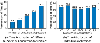
Figure 9. Benchmark profile.

Evaluation Metrics. We use the following two metrics to evaluate the scheduling performance.

• Inference Accuracy Gain. Since the absolute top-1 accuracies obtained by the six applications are not in the same range, we thus use accuracy gain over the baseline within each application as a more meaningful metric.

• Frame Rate Speedup. Similarly, since the absolute frame rate achieved depends on the number of concurrently running applications, we thus use frame rate speedup over the baseline as a more meaningful metric.

4.3.2. Improvement on Inference Accuracy and Frame Rate

Figure 10(a) compares the runtime performance between NestDNN and the baseline under the MinTotalCost scheduling scheme. The yellow circle represents the runtime performance of the baseline. Each blue diamond marker represents the runtime performance obtained by scheduling with a particular $\alpha$ in the cost function defined in Equation (2).

We have two key observations from the result. First, by adjusting the value of $\alpha$, NestDNN is able to provide various trade-offs between inference accuracy and frame rate, which the status quo approach could not provide. Second, the vertical and horizontal dotted lines altogether partition the figure into four quadrants. The upper right quadrant represents a region where NestDNN achieves both higher top-1 accuracy and frame rate than the status quo approach. In particular, we select 3 blue diamond markers within the upper right quadrant to demonstrate the runtime performance improvement achieved by NestDNN. Specifically, when NestDNN has the same average top-1 accuracy as the baseline, NestDNN achieves $2.0\times$ average frame rate speedup compared to the baseline. When NestDNN has the same average frame rate as the baseline, NestDNN achieves $4.1\%$ average accuracy gain compared to the baseline. Finally, we select the “knee” of the blue diamond curve, which offers the best accuracy-frame rate trade-off among all the $\alpha$. At the “knee”, NestDNN achieves $1.5\times$ average frame rate speedup and $2.6\%$ average accuracy gain compared to the baseline.

Figure 10(b) compares the runtime performance between NestDNN and the baseline under the MinMaxCost scheduling scheme. When NestDNN has the same average top-1 accuracy gain as the baseline, NestDNN achieves $1.9\times$ average frame rate speedup compared to the baseline. When NestDNN has the same average frame rate as the baseline, NestDNN achieves $4.2\%$ average accuracy gain compared to the baseline. At the “knee”, NestDNN achieves $1.5\times$ average frame rate speedup and $2.1\%$ average accuracy gain compared to the baseline.

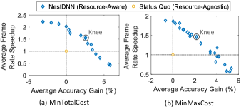
Figure 10. Runtime performance comparison between NestDNN (resource-aware) and status quo (resource-agnostic) under (a) MinTotalCost and (b) MinMaxCost.

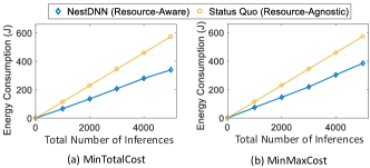
Figure 11. Energy consumption comparison between NestDNN (resource-aware) and status quo (resource-agnostic) under (a) MinTotalCost and (b) MinMaxCost.

4.3.3. Reduction on Energy Consumption

Besides improvement on inference accuracy and frame rate, NestDNN also consumes less energy. Figure 11(a) compares the energy consumption between NestDNN at the “knee” and the baseline under the MinTotalCost scheduling scheme. Across different numbers of inferences, NestDNN achieves an average $1.7\times$ energy consumption reduction compared to the baseline. Similarly, Figure 11(b) shows the comparison under the MinMaxCost scheduling scheme. NestDNN is able to achieve an average $1.5\times$ energy consumption reduction compared to the baseline.

5. Discussion

Impact on Mobile Vision Systems. NestDNN represents the first framework that supports resource-aware multi-tenant on-device deep learning for mobile vision systems. This is achieved by replacing fixed resource-accuracy trade-offs with flexible ones and dynamically selecting the optimal trade-off at runtime to deliver the maximum performance subject to resource constraint. We envision NestDNN could become a useful framework for future mobile vision systems.

Generality of NestDNN. In this work, we selected VGG Net and ResNet as two representative deep learning models to implement and evaluate NestDNN. However, NestDNN can be generalized to support many other popular deep learning models such as GoogLeNet (Szegedy et al., 2015), MobileNets (Howard et al., 2017), and BinaryNet (Courbariaux et al., 2016). NestDNN can also be generalized to support other computing tasks beyond computer vision tasks. In this sense, NestDNN is a generic framework for achieving resource-aware multi-tenant on-device deep learning.

Limitation. NestDNN in the current form has some limitation. Although our TRR approach outperforms the $\mathcal{L}1$-norm approach in filter pruning, its computational cost is much higher than $\mathcal{L}1$-norm. This significantly increases the cost of the multi-capacity model generation process, even though the process is only performed once. We will find ways to reduce the cost and leave it as our future work.

6. Related Work

Deep Neural Network Model Compression. Model compression for deep neural networks has attracted a lot of attentions in recent years due to the imperative demand on running deep learning models on mobile systems. One of the most prevalent methods for compressing deep neural networks is pruning. Most widely used pruning approaches focus on pruning model parameters (Han et al., 2015a, b). Although pruning parameters is effective at reducing model sizes, it does not necessarily reduce computational costs (Luo et al., 2017; Molchanov et al., 2016; Li et al., 2016), making it less useful for mobile systems which need to provide real-time services. To overcome this problem, Li et al. (Li et al., 2016) proposed a filter pruning method that has achieved up to $38\%$ reduction in computational cost. Our work also focuses on compressing deep neural networks via filter pruning. Our proposed filter pruning approach outperforms the state-of-the-art. Moreover, unlike existing model compression methods which produce pruned models with fixed resource-accuracy trade-offs, our proposed multi-capacity model is able to provide dynamic resource-accuracy trade-offs. This is similar to the concept of dynamic neural networks in the deep learning literature (Guo et al., 2016; Lin et al., 2017; Huang et al., 2017).

Continuous Mobile Vision. The concept of continuous mobile vision was first advanced by Bahl et al. (Bahl et al., 2012). The last few years have witnessed many efforts towards realizing the vision of continuous mobile vision (LiKamWa and Zhong, 2015; Han et al., 2016; Mathur et al., 2017; Huynh et al., 2017). In particular, in (LiKamWa and Zhong, 2015), LiKamWa et al. proposed a framework named Starfish, which enables efficient running concurrent vision applications on mobile devices by sharing common computation and memory objects across applications. Our work is inspired by Starfish in terms of sharing. By sharing parameters among descendent models, our proposed multi-capacity model has a compact memory footprint and incurs little model switching overhead. Our work is also inspired by (Han et al., 2016). In (Han et al., 2016), Han et al. proposed a framework named MCDNN, which applies various model compression techniques to generate a catalog of model variants to provide different resource-accuracy trade-offs. However, in MCDNN, the generated model variants are independent of each other, and it relies on cloud connectivity to retrieve the desired model variant. In contrast, our work focuses on developing an on-device deep learning framework which does not rely on cloud connectivity. Moreover, MCDNN focuses on model sharing across concurrently running applications. In contrast, NestDNN treats each of the concurrently running applications independently, and focuses on model sharing across different model variants within each application.

7. Conclusion

In this paper, we presented the design, implementation and evaluation of NestDNN, a framework that enables resource-aware multi-tenant on-device deep learning for mobile vision systems. NestDNN takes the dynamics of runtime resources in a mobile vision system into consideration, and dynamically selects the optimal resource-accuracy trade-off and resource allocation for each of the concurrently running deep learning models to jointly maximize their performance. We evaluated NestDNN using six mobile vision applications that target some of the most important vision tasks for mobile vision systems. Our results show that NestDNN outperforms the resource-agnostic status quo approach in inference accuracy, video frame processing rate, and energy consumption. We believe NestDNN represents a significant step towards turning the envisioned continuous mobile vision into reality.

8. Acknowledgement

We thank the anonymous shepherd and reviewers for their valuable feedback. This work was partially supported by NSF Awards CNS-1617627, IIS-1565604, and PFI:BIC-1632051.

References

- (1)
- mon (2016) 2016. Monsoon Power Monitor. https://www.msoon.com/LabEquipment/PowerMonitor/.
- nvi (2016) 2016. This Powerful Wearable Is a Life-Changer for the Blind. https://blogs.nvidia.com/blog/2016/10/27/wearable-device-for-blind-visually-impaired/.
- app (2017) 2017. An On-device Deep Neural Network for Face Detection. https://machinelearning.apple.com/2017/11/16/face-detection.html.
- ama (2018) 2018. Amazon DeepLens. https://aws.amazon.com/deeplens/.
- goo (2018) 2018. Google Clips. https://store.google.com/us/product/google_clips.
- Bahl et al. (2012) Paramvir Bahl, Matthai Philipose, and Lin Zhong. 2012. Vision: cloud-powered sight for all: showing the cloud what you see. In ACM workshop on Mobile cloud computing and services. 53–60.
- Courbariaux et al. (2016) Matthieu Courbariaux, Itay Hubara, Daniel Soudry, Ran El-Yaniv, and Yoshua Bengio. 2016. Binarized neural networks: Training deep neural networks with weights and activations constrained to+ 1 or-1. arXiv preprint arXiv:1602.02830 (2016).
- Fang et al. (2017) Biyi Fang, Jillian Co, and Mi Zhang. 2017. DeepASL: Enabling Ubiquitous and Non-Intrusive Word and Sentence-Level Sign Language Translation. In ACM SenSys. Delft, The Netherlands.
- Guo et al. (2016) Yiwen Guo, Anbang Yao, and Yurong Chen. 2016. Dynamic network surgery for efficient dnns. In NIPS. 1379–1387.
- Han et al. (2015a) Song Han, Huizi Mao, and William J Dally. 2015a. Deep compression: Compressing deep neural networks with pruning, trained quantization and huffman coding. arXiv preprint arXiv:1510.00149 (2015).
- Han et al. (2015b) Song Han, Jeff Pool, John Tran, and William Dally. 2015b. Learning both weights and connections for efficient neural network. In NIPS. 1135–1143.
- Han et al. (2016) Seungyeop Han, Haichen Shen, Matthai Philipose, Sharad Agarwal, Alec Wolman, and Arvind Krishnamurthy. 2016. MCDNN: An Approximation-Based Execution Framework for Deep Stream Processing Under Resource Constraints. In ACM MobiSys. 123–136.
- He et al. (2016) Kaiming He, Xiangyu Zhang, Shaoqing Ren, and Jian Sun. 2016. Deep residual learning for image recognition. In Proceedings of the IEEE Conference on Computer Vision and Pattern Recognition. 770–778.
- Howard et al. (2017) Andrew G Howard, Menglong Zhu, Bo Chen, Dmitry Kalenichenko, Weijun Wang, Tobias Weyand, Marco Andreetto, and Hartwig Adam. 2017. Mobilenets: Efficient convolutional neural networks for mobile vision applications. arXiv preprint arXiv:1704.04861 (2017).
- Huang et al. (2017) Gao Huang, Zhuang Liu, Kilian Q Weinberger, and Laurens van der Maaten. 2017. Densely connected convolutional networks. In IEEE conference on computer vision and pattern recognition, Vol. 1. 3.
- Huh et al. (2016) Minyoung Huh, Pulkit Agrawal, and Alexei A Efros. 2016. What makes ImageNet good for transfer learning? arXiv:1608.08614 (2016).
- Huynh et al. (2017) Loc N. Huynh, Youngki Lee, and Rajesh Krishna Balan. 2017. DeepMon: Mobile GPU-based Deep Learning Framework for Continuous Vision Applications. In ACM MobiSys. 82–95.
- Krizhevsky and Hinton (2009) Alex Krizhevsky and Geoffrey Hinton. 2009. Learning multiple layers of features from tiny images. Technical Report. Citeseer.
- Krizhevsky et al. (2012) Alex Krizhevsky, Ilya Sutskever, and Geoffrey E Hinton. 2012. Imagenet classification with deep convolutional neural networks. In NIPS. 1097–1105.
- Lane et al. (2016) Nicholas D Lane, Sourav Bhattacharya, Petko Georgiev, Claudio Forlivesi, Lei Jiao, Lorena Qendro, and Fahim Kawsar. 2016. DeepX: A software accelerator for low-power deep learning inference on mobile devices. In ACM/IEEE IPSN. 1–12.
- LeCun et al. (2015) Yann LeCun, Yoshua Bengio, and Geoffrey Hinton. 2015. Deep learning. Nature 521, 7553 (2015), 436–444.
- Levi and Hassner (2015) Gil Levi and Tal Hassner. 2015. Age and gender classification using convolutional neural networks. In Proceedings of the IEEE Conference on Computer Vision and Pattern Recognition Workshops. 34–42.
- Li et al. (2016) Hao Li, Asim Kadav, Igor Durdanovic, Hanan Samet, and Hans Peter Graf. 2016. Pruning filters for efficient convnets. arXiv preprint arXiv:1608.08710 (2016).
- LiKamWa and Zhong (2015) Robert LiKamWa and Lin Zhong. 2015. Starfish: Efficient concurrency support for computer vision applications. In ACM MobiSys. 213–226.
- Lin et al. (2017) Ji Lin, Yongming Rao, Jiwen Lu, and Jie Zhou. 2017. Runtime neural pruning. In NIPS. 2181–2191.
- Luo et al. (2017) Jian-Hao Luo, Jianxin Wu, and Weiyao Lin. 2017. Thinet: A filter level pruning method for deep neural network compression. arXiv preprint arXiv:1707.06342 (2017).
- Mathur et al. (2017) Akhil Mathur, Nicholas D Lane, Sourav Bhattacharya, Aidan Boran, Claudio Forlivesi, and Fahim Kawsar. 2017. Deepeye: Resource efficient local execution of multiple deep vision models using wearable commodity hardware. In ACM MobiSys. 68–81.
- Molchanov et al. (2016) Pavlo Molchanov, Stephen Tyree, Tero Karras, Timo Aila, and Jan Kautz. 2016. Pruning convolutional neural networks for resource efficient transfer learning. arXiv preprint arXiv:1611.06440 (2016).
- Naderiparizi et al. (2017) Saman Naderiparizi, Pengyu Zhang, Matthai Philipose, Bodhi Priyantha, Jie Liu, and Deepak Ganesan. 2017. Glimpse: A Programmable Early-Discard Camera Architecture for Continuous Mobile Vision. In ACM MobiSys. 292–305.
- Oquab et al. (2014) Maxime Oquab, Leon Bottou, Ivan Laptev, and Josef Sivic. 2014. Learning and transferring mid-level image representations using convolutional neural networks. In IEEE CVPR. 1717–1724.
- Puri (2005) Anuj Puri. 2005. A survey of unmanned aerial vehicles (UAV) for traffic surveillance. Department of computer science and engineering, University of South Florida (2005), 1–29.
- Russakovsky et al. (2015) Olga Russakovsky, Jia Deng, Hao Su, Jonathan Krause, Sanjeev Satheesh, Sean Ma, Zhiheng Huang, Andrej Karpathy, Aditya Khosla, Michael Bernstein, et al. 2015. Imagenet large scale visual recognition challenge. International Journal of Computer Vision 115, 3 (2015), 211–252.
- Simonyan and Zisserman (2014) Karen Simonyan and Andrew Zisserman. 2014. Very deep convolutional networks for large-scale image recognition. arXiv preprint arXiv:1409.1556 (2014).
- Stallkamp et al. (2012) Johannes Stallkamp, Marc Schlipsing, Jan Salmen, and Christian Igel. 2012. Man vs. computer: Benchmarking machine learning algorithms for traffic sign recognition. Neural networks 32 (2012), 323–332.
- Sze et al. (2017) Vivienne Sze, Yu-Hsin Chen, Tien-Ju Yang, and Joel S Emer. 2017. Efficient processing of deep neural networks: A tutorial and survey. Proc. IEEE 105, 12 (2017), 2295–2329.
- Szegedy et al. (2015) Christian Szegedy, Wei Liu, Yangqing Jia, Pierre Sermanet, Scott Reed, Dragomir Anguelov, Dumitru Erhan, Vincent Vanhoucke, and Andrew Rabinovich. 2015. Going deeper with convolutions. In IEEE Conference on Computer Vision and Pattern Recognition. 1–9.
- Taigman et al. (2014) Yaniv Taigman, Ming Yang, Marc’Aurelio Ranzato, and Lior Wolf. 2014. Deepface: Closing the gap to human-level performance in face verification. In IEEE CVPR. 1701–1708.
- Zeng et al. (2017) Xiao Zeng, Kai Cao, and Mi Zhang. 2017. MobileDeepPill: A small-footprint mobile deep learning system for recognizing unconstrained pill images. In ACM MobiSys. 56–67.
- Zhang et al. (2017) Haoyu Zhang, Ganesh Ananthanarayanan, Peter Bodik, Matthai Philipose, Paramvir Bahl, and Michael J Freedman. 2017. Live Video Analytics at Scale with Approximation and Delay-Tolerance.. In NSDI.
- Zhou et al. (2017) Bolei Zhou, Agata Lapedriza, Aditya Khosla, Aude Oliva, and Antonio Torralba. 2017. Places: A 10 million Image Database for Scene Recognition. IEEE Transactions on Pattern Analysis and Machine Intelligence (2017).
- Zhou et al. (2014) Bolei Zhou, Agata Lapedriza, Jianxiong Xiao, Antonio Torralba, and Aude Oliva. 2014. Learning deep features for scene recognition using places database. In NIPS. 487–495.