Remote control of chemistry in optical cavities

Abstract

Manipulation of chemical reactivity often involves changing reagents or environmental conditions. Alternatively, strong coupling between light and matter offers a way to tunably hybridize their physicochemical properties and thereby change reaction dynamics without synthetic modifications to the starting material. Here, we theoretically design a polaritonic (hybrid photonic-molecular) device that supports ultrafast tuning of reaction yields even when the catalyst and its reactant are spatially separated across several optical wavelengths. We demonstrate how photoexcitation of a ‘remote catalyst’ in an optical microcavity can control photochemistry of a reactant in another microcavity. Harnessing delocalization across the spatially separated compounds that arises from strong cavity-molecule coupling, this intriguing phenomenon is shown for the infrared-induced cis $\rightarrow$ trans conformational isomerization of nitrous acid (HONO). Indeed, increasing the excited-state population of the remote catalyst can enhance the isomerization efficiency by an order of magnitude. The theoretical proposal reported herein is generalizable to other reactions and thus introduces a versatile tool to control photochemistry.

In photochemistry, energy transfer from light to matter produces nonequilibrium distributions of molecular states, therefore enabling selective initiation of reactive trajectories. For a given reaction, tuning of yields is commonly achieved by surveying a series of chemical analogs. These compounds undergo the same process but on different potential energy surfaces. The ability to synthesize substrates with sufficiently varying energetics, though, limits the range of accessible yields.

More facile chemical control of photoinduced reactivity is attainable in the strong couplingTörmä and Barnes (2015) limit. In this regime, energy coherently oscillates between light and matter faster than the rates at which their respective excitations decay, and the photonic and molecular states hybridize into polariton statesAgranovich et al. (2011). To reach sufficiently strong interaction between light and matter, ensembles of molecules can be placed in optical microcavities (Fig. 1)Agranovich et al. (2011). These nano- or microstructures support electromagnetic modes that form polaritons with molecular superpositions of the same symmetry as the spatial profile of the electric field. Importantly, the majority of linear combinations of matter energy states do not possess the right symmetry to mix with light (in realistic systems, slight mixing occurs due to symmetry-breaking environments; for example, see ref. Neuman and Aizpurua (2018)) and constitute the reservoir of dark states, which remains centered at the original molecular transition energy and plays a crucial role in the relaxation dynamics of polaritonsAgranovich et al. (2011); Ebbesen (2016); Ribeiro et al. (2018a). The energetic consequences and resulting reactivity of molecular polaritons have seen a surge in interest over the past several yearsEbbesen (2016); Feist et al. (2017); Ribeiro et al. (2018a); Flick et al. (2018); Schäfer et al. (2018). Since the observation of suppressed conversion between spiropyran and merocyanine organic dyesHutchison et al. (2012), modified kinetics upon polariton formation have been demonstrated in a wide variety of photochemical processes by experimental (reverse intersystem crossingStranius et al. (2018), photobleachingMunkhbat et al. (2018), triplet-triplet annihilationPolak et al. (2018), water splittingShi et al. (2018)), theoretical (charge transferHerrera and Spano (2016); Groenhof and Toppari (2018), dissociationKowalewski et al. (2016); Vendrell (2018), isomerizationGalego et al. (2016), singlet fissionMartínez-Martínez et al. (2018)), or both types of studies (energy transferZhong et al. (2017); Du et al. (2018); Sáez-Blázquez et al. (2018); Reitz et al. (2018); Schachenmayer et al. (2015)). In addition to detuning the cavity from molecular resonances, polaritonic systems offer a robust control knob of reaction energetics: reactant concentration $N/V$ (more precisely, $N$ is the total number of cavity-coupled reactant transitions and $V$ is the cavity mode volume) Ebbesen (2016); Feist et al. (2017); Ribeiro et al. (2018a); Flick et al. (2018). Indeed, the dependence of light-matter coupling strength, and the concomitant polaritonic energy splittings (Fig. 2), on $\sqrt{N/V}$ has enabled concentration-controlled tuning of a number of the aforementioned processesHutchison et al. (2012); Zhong et al. (2017); Stranius et al. (2018). While robust compared to substituting the reactant species, changing the concentration is still prone to issues of unfavorable intermolecular interactions, particularly insolubility.

Another convenient way to modulate the light-matter coupling is laser-driven ultrafast population of the dark-state reservoirDunkelberger et al. (2016, 2018); Xiang et al. (2018); Ribeiro et al. (2018b). In pump-probe spectroscopy of vibrational polaritons, the pump excitation of the polaritons is followed by subsequent relaxation into the dark-state reservoir within $\sim$10-100 ps delay time. This excited-state reservoir, owing to its large density of almost purely vibrational states, acts as a very efficient energy sink for the polaritonsdel Pino et al. (2015). Due to vibrational anharmonicity, the 1 $\rightarrow$ 2 transitions are detuned from the 0 $\rightarrow$ 1 transitions and therefore do not couple as well to cavity modes that are resonant with the latter. In other words, the concentration $N/V$ of molecular transitions that can strongly couple to the cavity mode is effectively reduced on an ultrafast timescale. The reduction is tuned by varying the intensity of the pump and detected in the frequency-resolved transient transmission of the probe pulseDunkelberger et al. (2018); Xiang et al. (2018).

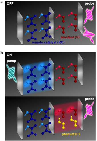
Figure 1: Optical microcavities enable remote control of infrared-induced conformational isomerization of HONO. a, Reaction is off. Without excitation of ‘remote catalyst’ (RC, blue molecule) Tc-glyoxylic acid, a ‘probe’ laser pulse impinging on the cavity containing reactant (R, red molecule) cis-HONO is off-resonant with polaritons and thereby reflected; no reaction occurs. b, Reaction is on. First, a ‘pump’ laser pulse impinging on the mirror of the RC cavity excites a polariton whose character is predominantly the RC cavity and the strongly coupled OH stretch (light blue bond) of RC. Next, the probe pulse is now able to efficiently excite a polariton whose character is predominantly the R cavity (light red) and the strongly coupled OH stretch (light red bond) of R; R subsequently converts into the product molecule (P, yellow molecule) trans-HONO.

Here we theoretically demonstrate ultrafast and remote tuning of reaction yields of the infrared-induced cis $\rightarrow$ trans fast isomerization channel of nitrous acid (HONO)Schanz et al. (2005). Observed in solid Kr matrices using ultrafast spectroscopy, this reaction is initiated by excitation of the OH stretch vibration of the cis (reactant) conformer. Product formation happens on a 20 ps timescale with an appreciable quantum yield of 10%. Therefore, this isomerization should serve as an ideal candidate to study photoinduced processes involving vibrational polaritons, given that typical infrared-optical microcavities are sufficiently long-lived ($\sim$1-10 ps)Dunkelberger et al. (2016, 2018); Xiang et al. (2018) to accommodate the described chemical transformation. We propose a polaritonic device (Fig. 1) that consists of two microcavities containing respectively ‘remote catalyst’ (RC) Tc-glyoxylic acidOlbert-Majkut et al. (2014a, b) (Supplementary Note 1) and reactant (R) cis-HONO. Strong coupling exists between the OH stretch ensembles of the molecules and their corresponding host microcavities, as well as between the microcavitiesStanley et al. (1994). The resulting polaritonic eigenstates are delocalized among both RC and R molecules. It follows that without any direct interaction between the two molecular species, pump-driven population of the RC dark-state reservoir can modify the energetics of R and thereby its reactivity in probe-driven conversion to product (P) trans-HONO (Fig. 1, cf. a and b). Specifically, the probe pulse—which impinges on the R cavity—can be set off-resonant with polaritons with R character such that pumping—with a pulse impinging on the RC cavity—shifts them into resonance (Fig. 2, cf. a and b). By increasing the pump field intensity, this nonlocal strategy can tune reaction efficiency by an order of magnitude.

Results

To model ultrafast tuning of the photoinitiated R $\rightarrow$ P conversion, we first describe the bare reaction (i.e., that without strong light-matter coupling) as comprising three steps. The first is absorption of light to create a single OH stretch excitation in R, which we label with $|\text{R}\rangle$ (see Methods). The second step is intramolecular vibrational redistribution (IVR, Nesbitt and Field (1996)) transition from $|\text{R}\rangle$ to the near-resonant seventh overtone mode of the torsional coordinate. Given the proximity of this highly excited state to the barrier of the torsional double-well potential energy surface and its consequent delocalization across R and PSchanz et al. (2005), the third step is relaxation into the R and P local well via interaction with matrix degrees of freedom. For simplicity of notation, we hereby refer to the product-yielding overtone state as $|\text{P}\rangle$, although it should be clear that it has mixed character of R and P. This mechanism is in line with that first proposed for the reaction induced by pulsedSchanz et al. (2005) and continuous-waveHall and Pimentel (1963) excitation, and is in qualitative agreement with mechanisms suggested by later studies (Supplementary Note 2).

Having addressed the main features of the reaction in the conventional photochemical setting, we next proceed to describe it within the context of the proposed device, where the probe absorption into the polariton states triggers IVR onto $|\text{P}\rangle$. Both absorption and IVR are treated with a version of input-output theoryGardiner and Collett (1985); Ciuti and Carusotto (2006); Li et al. (2017) adapted to pump-probe spectroscopy for vibrational polaritonsRibeiro et al. (2018b) (Supplementary Note 4). In this approach, the pump-induced population of dark reservoir states, denoted by an effective fraction $f_{\text{pump}}$ of the total number of molecules $N$ in the molecular ensemble, controls the nonlinear spectral features. The major qualitative and quantitative features of experimental transient spectra are captured within this theoryXiang et al. (2018); Ribeiro et al. (2018b)—including the frequencies and intensities of the resonances exhibited by the transient transmission of the probe. In this work, we disregard electrical anharmonicityRibeiro et al. (2018b) (and fine-structure contributions such as molecular rotationsĆwik et al. (2016); Szidarovszky et al. (2018)), whose inclusion should not qualitatively change our main findings.

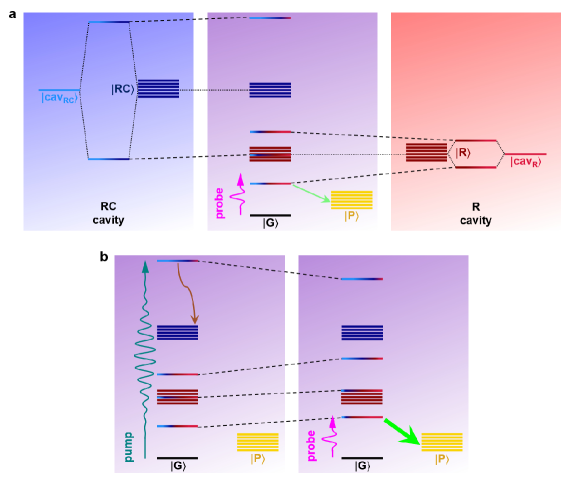
Figure 2: Pumping of the ‘remote catalyst’ (RC) modifies reaction energetics. a, (Blue and red panels) Represented by dotted lines, strong coupling between cavity photon $|\text{cav}_{\text{RC}}\rangle$ ($|\text{cav}_{\text{R}}\rangle$) and the OH stretch $|\text{RC}\rangle$ ($|\text{R}\rangle$) in $N$ molecules of RC (reactant, R) produces two polaritons and $N-1$ dark states; $N=6$ is depicted here for illustration. (Purple panel) Intercavity coupling further hybridizes (dashed lines) the photonic and vibrational states into polaritons of the entire light-matter device. A probe excitation is off-resonant with the lowest polariton, affording inefficient transfer (thin green arrow) into product-yielding state $|\text{P}\rangle$. b, (Left panel) Pump excitation of the highest polariton is followed by relaxation (brown arrow) into the RC dark states during a < 100 ps delay time. Owing to anharmonicities, this pumping reduces the collective $|\text{RC}\rangle$-$|\text{cav}_{\text{RC}}\rangle$ interaction and modifies (dashed lines) the polaritons within an ultrafast timescale. (Right panel) The probe excitation is now resonant with the lowest polariton, which has increased mixing fraction of R and its cavity, affording efficient transfer (thick green arrow) into $|\text{P}\rangle$. In both a and b, $|\text{G}\rangle$ is the molecular and photonic vacuum ground state (energy not drawn to scale), and the polariton vertical positions (color gradients) represents their energies (mixing fractions) (see Supplementary Note 6).

Before proceeding to analyze the dynamics of the remote-control device, we investigate its spectral features. In the first excitation manifold, the Hamiltonian for the polariton states in the basis of the constituent species is ($\hbar=1$)

$$H_{\text{system}}^{(\text{no pump})}=\begin{pmatrix}\omega_{\text{RC}}&g_{\text{RC}}\sqrt{N_{\text{RC}}}&0&0\\ g_{\text{RC}}\sqrt{N_{\text{RC}}}&\omega_{\text{cav}_{\text{RC}}}&g_{\text{cav}}&0\\ 0&g_{\text{cav}}&\omega_{\text{cav}_{\text{R}}}&g_{\text{R}}\sqrt{N_{\text{R}}}\\ 0&0&g_{\text{R}}\sqrt{N_{\text{R}}}&\omega_{\text{R}}\end{pmatrix},$$ (1)

where the entries from left to right (top to bottom) represent the OH stretch excitation in RC (labeled by $|\text{RC}\rangle$), the cavity hosting RC, the cavity hosting R, and $|\text{R}\rangle$, respectively. For simplicity, we take each cavity mode to be resonant with the hosted OH vibration: $\omega_{\text{cav}_{\text{RC}}}=\omega_{\text{RC}}=3455\text{ cm}^{-1}$ (the average frequency of the OH stretch of RCOlbert-Majkut et al. (2014b, a), see Supplementary Note 1) and $\omega_{\text{cav}_{\text{R}}}=\omega_{\text{R}}=3402\text{ cm}^{-1}$ (the frequency of the OH stretch vibration of RSchanz et al. (2005)). Let the collective light-matter couplingsRibeiro et al. (2018a) be $g_{\text{RC}}\sqrt{N_{\text{RC}}}=57\text{ cm}^{-1}$ and $g_{\text{R}}\sqrt{N_{\text{R}}}=11\text{ cm}^{-1}$ for numbers $N_{\text{RC}}$ and $N_{\text{R}}$ of RC and R molecules, respectively, per mode volume $V$ of each cavity; we have incorporated $V$ into the $g$ values for notational convenience. These couplings correspond to $\sim 1.7\%$ and $\sim 0.3\%$ of the transition energy of each interacting species, comparable to experimental values (0.2-2.2%) for mid-infrared vibrational polaritonsDunkelberger et al. (2018); Casey and Sparks (2016). With no cavity-cavity coupling ($g_{\text{cav}}=0$; Fig. 2a, blue and red panels), one pair of polaritons has character of only RC and its cavity (blue), and the other pair only R and its cavity (red). Upon introduction of intercavity coupling $g_{\text{cav}}=27\text{ cm}^{-1}$ (Fig. 2a, purple panel)—corresponding to $\sim 0.8\%$ of the cavity photon energiesStanley et al. (1994)—the three lowest polaritons from the $g_{\text{cav}}=0$ case hybridize into three states delocalized across RC, R, and their host cavities. This delocalization enables pumping of RC to remotely tune the energy of polaritons with R character and thereby the isomerization efficiency. In contrast, the highest polariton for $g_{\text{cav}}=0$ is spectrally isolated and does not change much in energy or character when intercavity coupling is introduced (Fig. 2a, cf. blue and purple panels).

Nevertheless, population of the dark RC states is achievable via excitation of this highest polariton with a pump pulse (Fig. 2b, left panel) impinging on the RC cavity (Fig. 1b, top panel). Given large enough $g_{\text{RC}}$ and $\omega_{\text{RC}}-\omega_{\text{R}}$, this highest level is essentially half RC and half RC cavity in character. Furthermore, by conservation of the number of energy levels, there are $N_{\text{RC}}-1$ RC dark reservoir states, significantly larger than 4, the number of polaritons. Downhill energy relaxation from the highest polariton is then most likely to occur into the relatively dense RC dark manifoldAgranovich et al. (2011); del Pino et al. (2015); Ribeiro et al. (2018a). In fact, this process is permitted in a matrix of Kr (Supplementary Fig. 3).

The resulting pump-dependent effective Hamiltonian isRibeiro et al. (2018b)

$$H_{\text{system}}^{(\text{pump})}=\begin{pmatrix}\omega_{\text{RC}}&0&g_{\text{RC}}\sqrt{(1-2f_{\text{pump}})N_{\text{RC}}}&0&0\\ 0&\omega_{\text{RC}}+2\Delta&g_{\text{RC}}\sqrt{2f_{\text{pump}}N_{\text{RC}}}&0&0\\ g_{\text{RC}}\sqrt{(1-2f_{\text{pump}})N_{\text{RC}}}&g_{\text{RC}}\sqrt{2f_{\text{pump}}N_{\text{RC}}}&\omega_{\text{cav}_{\text{RC}}}&g_{\text{cav}}&0\\ 0&0&g_{\text{cav}}&\omega_{\text{cav}_{\text{R}}}&g_{\text{R}}\sqrt{N_{\text{R}}}\\ 0&0&0&g_{\text{R}}\sqrt{N_{\text{R}}}&\omega_{\text{R}}\end{pmatrix}.$$ (2)

(see Supplementary Note 5 for derivation and interpretation). Though not utilized in calculations of absorption or reaction efficiency, this matrix provides physical intuition in that it characterizes the polaritonic transitions in the absence of lineshape broadening (our calculations do account for dissipative effects, see Methods): $|\text{RC}\rangle$, the $|\text{RC}\rangle$ 1 $\rightarrow$ 2 transition, the cavity with RC, the cavity with R, and $|\text{R}\rangle$, from left to right (top to bottom). $\Delta=-89\text{ cm}^{-1}$ is the mechanical anharmonicity of the OH stretch of RCOlbert-Majkut et al. (2014a, b) (Supplementary Note 1). It is evident from equation (2) that as the parameter $f_{\text{pump}}$ representing the degree of population of RC dark reservoir states is increased, the coupling between RC and the cavity is reduced, formalizing the qualitative arguments provided above. Taking the perspective that the hybrid states for $g_{\text{cav}}\neq 0$ are formed by mixing the polariton states of each cavity (when $g_{\text{cav}}=0$, Fig. 2a), pumping blueshifts the lower RC polariton away from the lower R polariton and reduces their mixing when $g_{\text{cav}}\neq 0$ (Fig. 2b, cf. left and right panels). Indeed, the lowest polariton for $g_{\text{cav}}\neq 0$ becomes predominantly R and its corresponding cavity upon pumping (Fig. 1b, right panel).

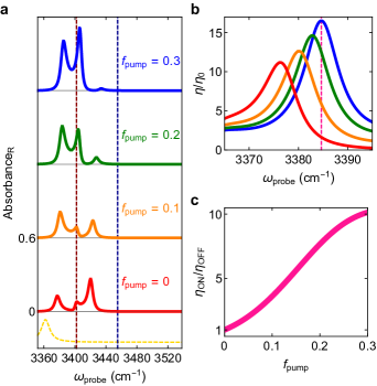
Figure 3: Pumping of the ‘remote catalyst’ (RC) turns on reaction with high tunability. a, Probe energy absorption into reactant (R) given various fractions $f_{\text{pump}}$ of pump-excited RC molecules. The dashed lines indicate the energies of the bare vibrations (i.e., those without strong light-matter coupling) of RC (dark blue) and R (dark red), as well as the arbitrarily scaled effective energy lineshape of the non-absorbing quantum state $|\text{P}\rangle$ (yellow) that first receives population from the strongly coupled R vibration via IVR and then relaxes into product (P) states (see main text). b, Relative reaction efficiency $\eta/\eta_{0}$ (i.e., compared to the bare efficiency) as a function of the ‘probe’ pulse energy. The color scheme for the solid lines follows that of a. c, Enhancement $\eta_{\text{ON}}/\eta_{\text{OFF}}$ of reaction efficiency (i.e., compared to $f_{\text{pump}}=0$) as a function of $f_{\text{pump}}$ at the probe energy ($\omega_{\text{probe}}\approx 3385\text{ cm}^{-1}$) is indicated by the pink dashed line in c.

The ability to shift its energy and increase its R character with pumping of RC renders this lowest polariton state promising for pump-enhancing the energy that eventually dissipates into R molecules, and thus the isomerization triggered when a probe pulse impinges on the R cavity (Fig. 2, cf. a and b). Spectra (Fig. 3a) computed from input-output theory (see Methods) reveal that probe absorption of the lowest polariton into R is stronger with more pumping. This trend is in agreement with the pump dependence of its R and R-cavity mixing fractions (Fig. 2b, cf. left and right panels). As a consistency check, we note that the energies and intensities of the other absorption peaks (Fig. 3a) also agree with the energies and R/R-cavity characters, respectively (Fig. 2).

Now we show that the reaction efficiency $\eta$ is highly pump-tunable (Fig. 3b). Also calculated from input-output theory (see Methods), $\eta$ (equation (14)) is the product of the probe absorbance into R and the quantum yield of isomerization from the excited polariton. Given that the peak absorption of the lowest polariton moves away in energy from $|\text{P}\rangle$ ($\omega_{\text{P}}=3362\text{ cm}^{-1}$Schanz et al. (2005), Supplementary Note 2) with pumping (Fig. 3a), it is somewhat counterintuitive that the corresponding peak value of $\eta$ increases. This behavior arises because for all values of $f_{\text{pump}}$, spectral overlap between any polariton and $|\text{P}\rangle$ is small (Fig. 3a). Thus, the peak $\eta$ is controlled by the position and intensity of the lowest-polariton absorption. It therefore makes sense that the maximum $\eta$ blueshifts and rises with higher pumping (Fig. 3b). Relative to the experimental bare reaction efficiency $\eta_{0}$ (see Methods), the $\eta$ values grow to an order of magnitude greater with increasing $f_{\text{pump}}$ (Fig. 3b). The reason for such high values is that the lowest polariton is a more efficient absorber (Fig. 3a) and is nearer in resonance to $|\text{P}\rangle$ compared to the bare $|\text{R}\rangle$ (peak absorbance = 0.07Schanz et al. (2005)). To realize remote tuning of reactivity, we focus on the probe frequency (Fig. 3b, pink dashed line) that corresponds to the peak $\eta$ for the highest explored fraction $f_{\text{pump}}=0.3$ of pump-excited RC molecules. Notably, pumping enhances the reaction efficiency $\eta_{\text{ON}}$ for this choice of $\omega_{\text{probe}}$ by over an order of magnitude compared to the efficiency $\eta_{\text{OFF}}$ with no pumping (Fig. 3c). As an aside, while uphill relaxation may happen from the lowest polariton to the dark R states, this interfering process can be minimized with lower temperatures. Even if the relaxation is significantly fast, e.g., compared to polariton decay, the isomerization and its enhancement can still be observed as long as polariton absorption is detectable.

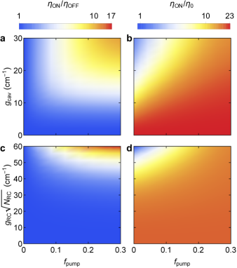
Figure 4: Pump-induced reaction enhancement can be remotely tuned by varying properties of the ‘remote catalyst’ (RC) and its host cavity. Reaction efficiencies $\eta_{\text{ON}}$ relative to those without pumping ($\eta_{\text{OFF}}$) or in the bare case (i.e., without strong light-matter coupling, $\eta_{0}$), respectively, as a function of either intercavity coupling strength $g_{\text{cav-cav}}$ (a and b) or collective cavity-RC coupling $g_{\text{RC}}\sqrt{N_{\text{RC}}}$ (c and d) and fraction $f_{\text{pump}}$ of pump-excited RC molecules. In b and d, notice the ability to control reaction efficiency even in the linear optical regime ($f_{\text{pump}}=0$).

So far, we have considered modifying a reaction by optical pumping of RC. We now briefly show further manipulation of the R $\rightarrow$ P isomerization efficiency via tuning of intercavity and cavity-RC couplings, both adjustable without any direct alteration of R. Thus, we also show remote control of the reaction in the linear probe-excitation regime, i.e., without pumping. When the intercavity coupling is manipulated (Fig. 4a), e.g., by varying the thickness of the middle mirrorSkolnick et al. (1998), the maximum boost in reaction efficiency with pumping ($\eta_{\text{ON}}$) over that without ($\eta_{\text{OFF}}$) reaches several tenfold as $g_{\text{cav}}$ rises from 0 to $30\text{ cm}^{-1}$. Such increase occurs because delocalization of the lowest polariton across RC, R, and their host cavities—and therefore potential for reactive modification— increases with intercavity coupling. Changing $g_{\text{cav}}$ raises too the absolute $\eta_{\text{ON}}$ (compared to bare efficiency $\eta_{0}$, Fig. 4b) by over an order of magnitude for fixed $f_{\text{pump}}$, especially when $f_{\text{pump}}=0$. Alternatively, $g_{\text{RC}}\sqrt{N_{\text{RC}}}$ can be tuned (Fig. 4c), e.g., by increasing the concentration of RC, to yield similar favorable pump-enhancements (Fig. 4, cf. a and c) and absolute efficiencies (Fig. 4, cf. b and d) for fixed pumping. Indeed, cavity-RC coupling too can regulate the efficiency of the single-pulse photoisomerization (Fig. 4b, $f_{\text{pump}}=0$). Notice though that $g_{\text{RC}}\sqrt{N_{\text{RC}}}$ must exceed $\sim 40\text{ cm}^{-1}$ to appreciably influence $\eta_{\text{ON}}/\eta_{\text{OFF}}$ (Fig. 4c) and $\eta_{\text{ON}}/\eta_{0}$ (Fig. 4d). The origin of this requirement is the same as that of the pump-induced modulation (with fixed cavity-RC coupling): adjusting $g_{\text{RC}}\sqrt{N_{\text{RC}}}$ changes the mixing between the polaritons of each cavity (when $g_{\text{cav}}=0$); control of reactivity is realizable when the lowest polariton of the entire device is sufficiently delocalized across the photonic and vibrational species associated with both RC and R. While pumping of RC provides a very versatile tuning mechanism, in the absence of ultrafast equipment and so long as increasing the thickness of the intercavity mirror or the concentration of RC is feasible, the linear optical experiments suggested provide an interesting alternative to our original proposal.

Discussion

We have theoretically demonstrated ultrafast remote control of the isomerization of cis-HONO to trans-HONO using an infrared polaritonic device. The proposed setup consists of two strongly interacting microcavities containing separate ensembles of ‘remote catalyst’ (RC) and reactant. The polaritons of the hybrid system are delocalized across both molecular species and their host cavities. Acting on the RC cavity, a pump pulse excites the highest polariton, followed by picosecond-timescale relaxation to the dark-state reservoir of RC. Due to anharmonicity, the 1 $\rightarrow$ 2 vibrational transitions of RC are significantly detuned from the RC cavity mode, hence inducing an effective weakening of the collective coupling (and hybridization) between RC and the remaining components of the device. The lowest polariton concomitantly acquires less character of RC and its respective cavity and more of reactant and its respective cavity. As a result, probe-pulse excitation acting on the reactant cavity yields enhanced efficiency of IVR into the product state compared to the no-pumping case. By raising the pump intensity, the reaction efficiency can be boosted by an order of magnitude. Remarkably, this tunability requires no spatial contact whatsoever between RC and reactant, challenging the paradigm of traditional chemical catalysis. We emphasize that additional manipulation of reactivity can be achieved by varying the intercavity or RC-cavity coupling strengths, e.g., by changing the distance between cavities or the concentration of RC, respectively. These adjustments extend remote control to the linear optical regime.

Although our results involve tuning a vibrational excited state that couples into the reaction coordinate, they can be generalized to electronic excited states, which feature a variety of photochemical reactions, some of which have been explored already in the polaritonic regimeEbbesen (2016); Feist et al. (2017); Ribeiro et al. (2018a); Flick et al. (2018). Success of the proposed strategies relies essentially on (1) the ability to couple RC and R to interacting cavity modes and (2) a difference in coupling between the fundamental and anharmonic transition of the former compound. Indeed, inorganicKhitrova et al. (1999) and organicVasa et al. (2013); Liu et al. (2015) excitons are satisfactory platforms for realization of the polaritonic device and the pump-dependent modulation of light-matter coupling studied here. Furthermore, remote control of reactivity can be extended to include plasmonic nanostructures, which have been well-studied in the strong coupling regimeBellessa et al. (2004); Törmä and Barnes (2015); Maxim and Abraham (2017) and also offer promising routes for ultrafast manipulation of nanoparticle-reactantFofang et al. (2011), plasmon-plasmonProdan et al. (2003), and photon-plasmon interactionsThakkar et al. (2017).

Beyond the application described here, the polaritonic device can be employed as a diagnostic tool for reaction mechanisms. For example, identification of states that afford high reactive tunability, when strongly coupled in the polaritonic device, can provide mechanistic insight. Such functionality would be especially attractive for processes that involve a series of state-to-state transitions, e.g., IVR or IVR-driven reactions such as the HONO isomerization studied here. More broadly, the proposed remote control represents a new class of molecular quantum technologies featuring manipulation of chemical processes through coherent interactionsShapiro and Brumer (2012). In addition, this technique to control reactions without direct catalyst-reactant interaction paves way for novel and possibly greener approaches to catalytic and separations chemistry.

Methods

Hamiltonian for polaritonic device

The Hamiltonian for the proposed polaritonic setup (Fig. 1) is $H=H_{\text{system}}+H_{\text{bath}}+H_{\text{system}-\text{bath}}$, where the latter two terms are provided in Supplementary Note 4, and

$$H_{\text{system}} =H_{\text{RC}}+H_{\text{cav}_{\text{RC}}}+H_{\text{cav}_{\text{RC}}-\text{RC}}$$

$$\quad+H_{\text{cav}_{\text{RC}}-\text{cav}_{\text{R}}}+H_{\text{R}}+H_{\text{cav}_{\text{R}}}+H_{\text{cav}_{\text{R}}-\text{R}}$$

$$\quad+H_{\text{P}}+H_{\text{R}-\text{P}},$$ (3)

from which Hamiltonian $H_{\text{system}}^{(\text{no pump})}$, equation (1), follows in the perturbative limit of $H_{\text{R}-\text{P}}$. From left to right and top to bottom, the terms of equation (1) respectively represent the contributions of RC, RC cavity, their coupling, intercavity coupling, R cavity, R, cavity-$|\text{R}\rangle$ coupling, P, and the $|\text{R}\rangle$-$|\text{P}\rangle$ IVR coupling. Explicitly, these terms read ($\hbar=1$)

$$H_{\text{RC}} =\omega_{\text{RC}}\sum_{i=1}^{N_{\text{RC}}}a_{\text{RC},i}^{\dagger}a_{\text{RC},i}$$ (4a)

$$\quad+\Delta\sum_{i=1}^{N_{\text{RC}}}a_{\text{RC},i}^{\dagger}a_{\text{RC},i}^{\dagger}a_{\text{RC},i}a_{\text{RC},i},$$ (4b)

$$H_{\text{cav}_{\text{RC}}} =\omega_{\text{cav}_{\text{RC}}}c_{\text{RC}}^{\dagger}c_{\text{RC}},$$ (5)

$$H_{\text{cav}_{\text{RC}}-\text{RC}} =g_{\text{RC}}\sum_{i=1}^{N_{\text{RC}}}(a_{\text{RC},i}^{\dagger}c_{\text{RC}}+\text{h.c.}),$$ (6)

$$H_{\text{cav}_{\text{RC}}-\text{cav}_{\text{R}}} =g_{\text{cav}}(c_{\text{R}}^{\dagger}c_{\text{RC}}+\text{h.c.}),$$ (7)

$$H_{\text{R}} =\omega_{\text{R}}\sum_{i=1}^{N_{\text{R}}}a_{\text{R},i}^{\dagger}a_{\text{R},i},$$ (8)

$$H_{\text{cav}_{\text{R}}} =\omega_{\text{cav}_{\text{R}}}c_{\text{R}}^{\dagger}c_{\text{R}},$$ (9)

$$H_{\text{P}} =\omega_{\text{P}}\sum_{i=1}^{N_{\text{R}}}|\text{$\text{P}_{i}\rangle$}\langle\text{P}_{i}|,$$ (10)

$$H_{\text{R}-\text{P}} =V_{\text{R}-\text{P}}\sum_{i=1}^{N_{\text{R}}}(|\text{P}_{i}\rangle\langle\text{G}|a_{\text{R},i}+\text{h.c.}).$$ (11)

Here, $a_{x,i}^{\dagger}$ ($a_{x,i}$) is the bosonic creation (annihilation) operator for an OH stretch excitation at the $i$th molecule of the $x=\text{RC},\,\text{R}$ species; $c_{x}^{\dagger}$ ($c_{x}$) is the bosonic creation (annihilation) operator for a photon in the cavity hosting $x$. Finally, $|\text{P}_{i}\rangle$ is the seventh overtone (eighth excited state) of HONO molecule $i$ that has mixed cis and trans character, and $|\text{G}\rangle$ is the molecular and photonic vacuum ground state. All energy and coupling parameters are defined in the main text, except for $V_{\text{R}-\text{P}}$ (see Supplementary Note 3). Given that population of just RC (but not R) is assumed to be excited by the pump, only its anharmonicity is relevant (see equation (4b)).

Input-output theory for simulating absorption and reaction efficiency

Following conventional input-output theoryGardiner and Collett (1985); Ciuti and Carusotto (2006); Li et al. (2017), as well as its adaptation to pump-probe spectroscopy of vibrational polaritonsRibeiro et al. (2018b), we write the Heisenberg-Langevin equations of motion for the probe-induced dynamics of the proposed polariton device (see Supplementary Note 4 for derivation and Supplementary Fig. 2 for schematic representation of the equations):

$$\frac{dP_{\text{RC}}(t)}{dt} =-i(\omega_{\text{RC}}-i\gamma_{\text{RC}}/2)P_{\text{RC}}(t)$$

$$\quad-ig_{\text{RC}}\sqrt{N_{\text{RC}}}c_{\text{RC}}(t)-2i\Delta P_{\text{RC},3}(t),$$ (12a)

$$\frac{dP_{\text{RC},3}(t)}{dt} =-i(\omega_{\text{RC}}+2\Delta-i3\gamma_{\text{RC}}/2)P_{\text{RC},3}(t)$$

$$\quad-2ig_{\text{RC}}f_{\text{pump}}\sqrt{N_{\text{RC}}}c_{\text{RC}}(t),$$ (12b)

$$\frac{dc_{\text{RC}}(t)}{dt} =-i(\omega_{\text{cav}_{\text{RC}}}-i\kappa_{\text{RC}}/2)c_{\text{RC}}(t)$$

$$\quad-ig_{\text{cav}}c_{\text{R}}(t)-ig_{\text{RC}}\sqrt{N_{\text{RC}}}P_{\text{RC}}(t),$$ (12c)

$$\frac{dc_{\text{R}}(t)}{dt} =-i(\omega_{\text{cav}_{\text{R}}}-i\kappa_{\text{R}}/2)c_{\text{R}}(t)-ig_{\text{cav}}c_{\text{RC}}(t)$$

$$\quad-ig_{\text{R}}\sqrt{N_{\text{R}}}P_{\text{R}}(t)-\sqrt{\kappa_{\text{R}}}c_{\text{R},\text{in}}(t),$$ (12d)

$$\frac{dP_{\text{R}}(t)}{dt} =-i(\omega_{\text{R}}-i\gamma_{\text{R}}/2)P_{\text{R}}(t)$$

$$\quad-ig_{\text{R}}\sqrt{N_{\text{R}}}c_{\text{R}}(t)-iV_{\text{R}-\text{P}}P_{\text{P}}(t),$$ (12e)

$$\frac{dP_{\text{P}}(t)}{dt} =-i[\omega_{\text{P}}-i(\Gamma_{cis}+\Gamma_{trans})/2]P_{\text{P}}(t)$$

$$\quad-iV_{\text{R}-\text{P}}P_{\text{R}}(t).$$ (12f)

Here, $P_{x}=\sum_{i=1}^{N_{x}}a_{x,i}/\sqrt{N_{x}}$ is the linear molecular polarization representing the collective bright molecular states $|\text{R}\rangle=P_{\text{R}}^{\dagger}|\text{G}\rangle$ and $|\text{RC}\rangle=P_{\text{RC}}^{\dagger}|\text{G}\rangle$ mentioned in the main text. $P_{x}$ is coupled to cavity polarization $c_{x}^{\dagger}$; $P_{\text{RC},3}=\sum_{i=1}^{N_{\text{RC}}}a_{\text{RC},i}^{\dagger}a_{\text{RC},i}a_{\text{RC},i}/\sqrt{N_{\text{RC}}}$ is the third-order polarization for RC that depends on the pump-induced excited-state fraction $f_{\text{pump}}$, a parameter that describes the extent of pumped RC population stored in the corresponding dark-state reservoir (see main text). The decay constants $\gamma_{\text{RC}}=\gamma_{\text{R}}=5\text{ cm}^{-1}$ approximate the absorption linewidth of the OH stretch excitation in RSchanz et al. (2005) and RCOlbert-Majkut et al. (2014b, a). The cavity photon lifetimes $\kappa_{\text{RC}}=\kappa_{\text{R}}=9.5\text{ cm}^{-1}$ are chosen such that $2\kappa_{x}/\omega_{x}$ (each cavity has only one mirror that couples to external photons, Fig. 1) approximately matches experimental parametersRibeiro et al. (2018b); Xiang et al. (2018). We have also defined the operator $P_{\text{P}}=\sum_{i=1}^{N_{\text{R}}}|\text{G}\rangle\langle\text{P}_{i}|/\sqrt{N_{\text{R}}}$ which keeps track of the IVR transferred population from $|\text{R}\rangle$ to $|\text{P}\rangle=P_{\text{P}}^{\dagger}|\text{G}\rangle$. The remaining decay rates $\Gamma_{cis}$ and $\Gamma_{trans}$ (Supplementary Note 3) represent relaxation of the HONO torsional state into the local R (cis) or P (trans) wells. The operator $c_{\text{R},\text{in}}$ represents the external probe field which couples into the system via the R cavity.

Carrying out the Fourier transform of equation (12), treating IVR as a perturbation in $V_{\text{R}-\text{P}}$ (Supplementary Note 4) and solving for $S_{\text{R}}(f_{\text{pump}},\omega)$ satisfying $P_{\text{R}}(\omega)=S_{\text{R}}(f_{\text{pump}},\omega)c_{\text{R},\text{in}}(\omega)$ allows for simulation (e.g., Fig. 3a in the main text) of the probe absorbance by R:

$$\text{absorbance}_{\text{R}}(f_{\text{pump}},\omega)=\gamma_{\text{R}}|S_{\text{R}}(f_{\text{pump}},\omega)|^{2}.$$ (13)

Doing the same steps with the P equation of motion gives the reaction efficiency

$$\eta(f_{\text{pump}},\omega)=\text{absorbance}_{\text{R}}(f_{\text{pump}},\omega)\text{QY}_{\text{R}\rightarrow\text{P}}(\omega),$$ (14)

where (Supplementary Note 3)

$$\text{QY}_{\text{R}\rightarrow\text{P}}(\omega) =\frac{\gamma_{\text{R}\rightarrow\text{P}}(\omega)}{\gamma_{\text{R}}}$$ (15)

is an isomerization quantum yield, and

$$\gamma_{\text{R}\rightarrow\text{P}}(\omega)=\frac{V_{\text{R}\rightarrow\text{P}}^{2}\Gamma_{trans}}{(\omega-\omega_{\text{P}})^{2}+[(\Gamma_{cis}+\Gamma_{trans})/2]^{2}}$$ (16)

is the transition rate from $|\text{R}\rangle$ to $|\text{P}\rangle$. The $\eta$ values discussed in the main text are defined as

$$\eta_{\text{ON}} =\eta(0.3,\omega_{\text{ON}}),$$ (17)

$$\eta_{\text{OFF}} =\eta(0,\omega_{\text{ON}}),$$ (18)

$$\eta_{0} \equiv\eta_{0}(\omega_{\text{R}}).$$ (19)

$\omega_{\text{ON}}$ (Fig. 3b, pink dashed line) is the frequency that maximizes $\eta(0.3,\omega)$ in the region $\omega\in[\omega_{\text{P}}-2\text{ cm}^{-1},\omega_{\text{R}}-g_{\text{R}}\sqrt{N_{\text{R}}}+2\text{ cm}^{-1}]$, containing the lowest polariton lineshape for all coupling strengths explored in this work. The derivation of $\eta_{0}(\omega)$ is given in Supplementary Note 3.

Author contributions

M.D. designed, carried out, and analyzed the calculations. R.F.R. guided the design and analysis of the calculations. J.Y.-Z. designed, conceived, and supervised the project. M.D. wrote the paper with input from all other authors.

Competing interests

The authors declare no competing interests.

Additional information

Supplementary information is available for this paper.
Correspondence and requests for materials should be addressed to J.Y.-Z.

Supplementary Notes for “Remote control of chemistry in optical cavities”

Matthew Du, Raphael F. Ribeiro, Joel Yuen-Zhou^∗

1 Tc-glyoxylic acid as choice of ‘remote catalyst’

The choice of the Tc conformer of glyoxylic acid Olbert-Majkut et al. (2014a, b) as the ‘remote catalyst’ (RC) is motivated by the following:

1. $|\text{RC}\rangle$ is an efficient absorber and should strongly couple to light given sufficient RC concentration,

2. the highest polariton of the device essentially has character of only RC and its cavity (Supplementary Fig. 4b),

3. solvent vibrational degrees of freedom mediate efficient relaxation between this highest polariton and RC dark states via one-phonon or multiphonon processes (Supplementary Fig. 3),

4. $|\text{RC}\rangle$ is photochemically stable (i.e., does not interconvert to conformers with different vibrational frequencies).

5. the lowest polariton of the device has significant character of R, RC, and their host cavities.

While excitation of the first overtone (second excited state) of Tc-glyoxylic acid induces a number of conformational reactions Olbert-Majkut et al. (2014b, a), these side processes can be safely neglected for this work. The 1$\rightarrow$2 $|\text{RC}\rangle$ transition of Tc-glyoxylic acid is sufficiently detuned from the 0 $\rightarrow$ 1 transitions of $|\text{R}\rangle$, $|\text{RC}\rangle$, and the strongly coupled cavity photons, such that the former transition contributes insignificantly to the polariton dynamics of the device.

To the best of our knowledge, the OH stretch frequency is not reported for Tc-glyoxylic acid in a Kr matrix, in which the fast-channel isomerization from R to P was observed Schanz et al. (2005). We thus approximate the frequency and anharmonic coupling constant of $|\text{RC}\rangle$ as averages of those for Tc-glyoxylic acid in Ar ($\omega_{10}=3473.5$ and $\Delta=-86$ $\text{cm}^{-1}$, respectively Olbert-Majkut et al. (2014b)) and Xe ($\omega_{10}=3436.5$ and $\Delta=-92$ $\text{cm}^{-1}$, respectively, for the conformer located in a ‘tight site’ of the Xe matrix Olbert-Majkut et al. (2014a)).

2 Isomerization model

In the main text, we considered the following mechanism for the fast isomerization pathway from R to P in a Kr matrix Schanz et al. (2005). Proceeding laser excitation, $|\text{R}\rangle$ first transfers energy via intramolecular vibrational redistribution (IVR) into $|\text{P}\rangle$, specifically the lower eigenstate that results (primarily) from mixing of the seventh localized torsional overtone of R and P Schanz et al. (2005). Then, $|\text{P}\rangle$ vibrationally relaxes into the localized potential wells of either R or P. This mechanism resembles those first proposed for the isomerization induced by pulsed Schanz et al. (2005) or continuous-wave Hall and Pimentel (1963) excitation. However, there is an alternative mechanism where $|\text{R}\rangle$ couples to a few discrete states that subsequently decay into continua, giving rise to P Hamm (2008). Nevertheless, the qualitative structure of the model is the same as the first one. Following the first mechanism for pulse-induced isomerization Schanz et al. (2005), we take $|\text{P}\rangle$ to be 40 cm^-1 lower in energy than $|\text{R}\rangle$. This energy gap (illustrated by the difference between the minima of potential energy curves 3 and 4 in Fig. 7 of Schanz et al. (2005)) was obtained by adjusting the barrier height of the torsional double well to a value ($3610\text{ cm}^{-1}$) that allows the potential energy curves of $|\text{R}\rangle$and $|\text{P}\rangle$ to cross Schanz et al. (2005).

3 Reaction efficiency in the absence of strong light-matter coupling

In this Supplementary Note, we calculate the efficiency of the fast isomerization from cis-HONO to trans-HONO in the bare case, i.e., in the absence of strong light-matter coupling. We apply input-output theory Gardiner and Collett (1985); Ciuti and Carusotto (2006); Steck (2007) to the reaction model described in the main text and in Supplementary Note 2. IVR from $|\text{R}\rangle$ to $|\text{P}\rangle$ is treated as a coupling between the two states, while the other reaction steps (e.g., absorption, relaxation into trans torsional potential well) are assumed to occur via coupling to a continuum of bath modes under the wide-band Nitzan (2006) approximation.

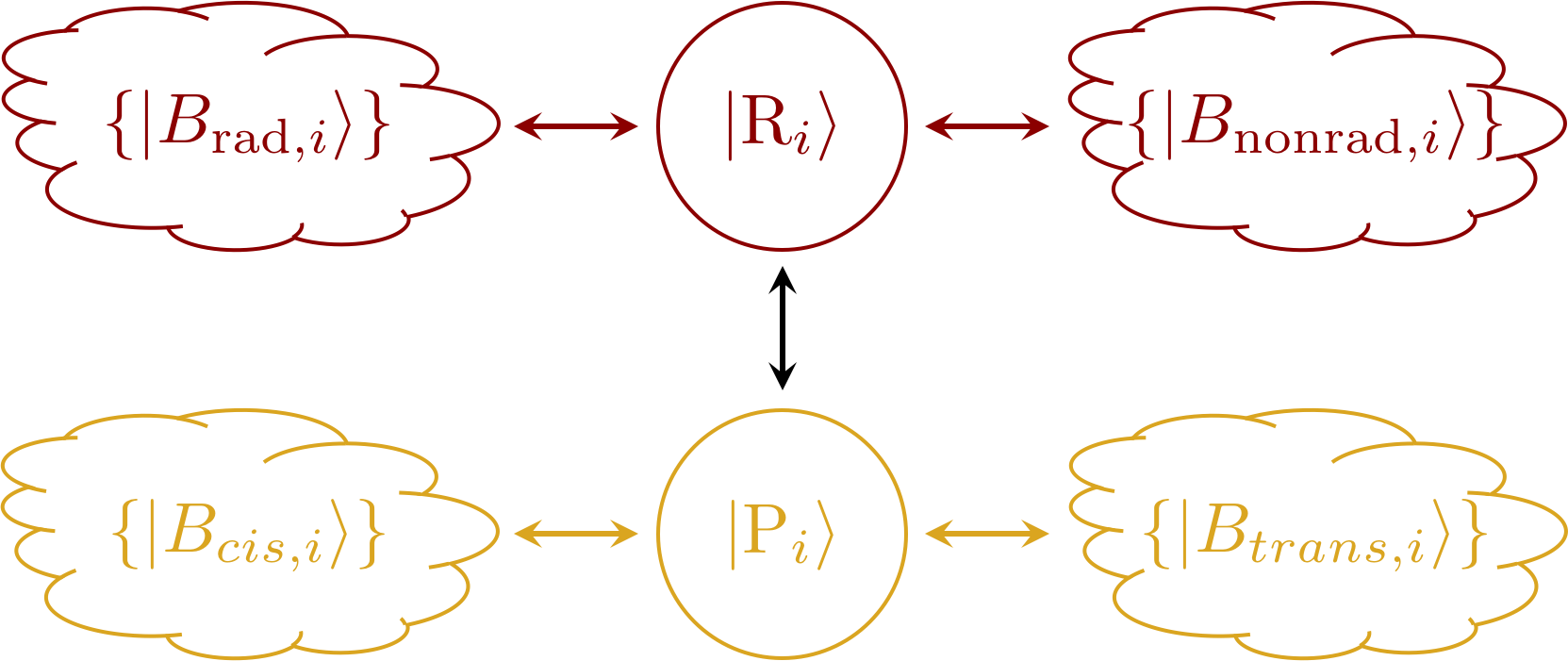
Supplementary Figure 1: Schematic of the system-bath interactions of the R $\rightarrow$ P fast isomerization channel in the absence of strong light-matter coupling. See equation (S1)) for the Hamiltonian $H_{0}$. The $i$th R molecule has an OH stretch $|\text{R}_{i}\rangle$ (dark red circle) which is coupled to a set ${|B_{\text{rad},i}\rangle}$ of radiative bath states (left dark red cloud) that contribute to its excitation and a set ${|B_{\text{nonrad},i}\rangle}$ of nonradiative bath states (right dark red cloud) that contribute to its decay. $|\text{R}_{i}\rangle$ is coupled to the torsional overtone state $|\text{P}_{i}\rangle$ (yellow circle), which can decay into either the $cis$ or $trans$ potential wells of HONO via coupling to ${|B_{cis,i}\rangle}$ (left yellow cloud) or ${|B_{trans,i}\rangle}$ (right yellow cloud), respectively.

Understanding that photonic bath modes induce excitation but nonradiative bath modes are the main contributors to relaxation of $|\text{R}\rangle$ Nitzan (2006), we can write the Hamiltonian as we did for the polaritonic device (Methods): $H_{0}=H_{\text{system},0}+H_{\text{bath},0}+H_{\text{system}-\text{bath},0}$. Specifically (hereafter, $\hbar=1$),

$$H_{\text{system},0} =H_{\text{R}}+H_{\text{P}}+H_{\text{R}-\text{P}},$$ (S1a)

$$H_{\text{bath},0} =\sum_{x=\text{rad},\text{nonrad}}\sum_{i=1}^{N_{\text{R}}}\int_{-\infty}^{\infty}d\omega\,\omega B_{x,i}^{\dagger}(\omega)B_{x,i}(\omega)+\sum_{y=cis,trans}\sum_{i=1}^{N_{\text{R}}}\int_{-\infty}^{\infty}d\omega\,\omega|B_{y,i}(\omega)\rangle\langle B_{y,i}(\omega)|,$$ (S1b)

$$H_{\text{system}-\text{bath},0} =\sum_{x=\text{rad},\text{nonrad}}\frac{\sqrt{\gamma_{x}}}{\sqrt{2\pi}}\sum_{i=1}^{N_{\text{R}}}\int_{-\infty}^{\infty}d\omega[a_{\text{R},i}^{\dagger}B_{x,i}(\omega)+\text{h.c.}]+\sum_{y=cis,trans}\frac{\sqrt{\Gamma_{y}}}{\sqrt{2\pi}}\sum_{i=1}^{N_{\text{R}}}\int_{-\infty}^{\infty}d\omega[|\text{P}_{i}\rangle\langle B_{y,i}(\omega)|+\text{h.c.}],$$ (S1c)

where $H_{\text{R}}$, $H_{\text{P}}$, and $H_{\text{R}-\text{P}}$ are defined respectively in equations (8), (10), and (11) of Methods. The various interactions between $|\text{R}_{i}\rangle=a_{\text{R},i}^{\dagger}|\text{G}\rangle$ , $|\text{P}_{i}\rangle$, and their baths are summarized in Fig. 1. $|\text{G}\rangle$ is the vacuum molecular ground state. The symbols $a_{\text{R},i}^{\dagger},|\text{P}_{i}\rangle$ and their Hermitian conjugates are defined in Methods. The bath modes are taken to be linearly coupled to $|\text{R}\rangle=\sum_{i=1}^{N_{\text{R}}}|\text{R}_{i}\rangle/\sqrt{N_{\text{R}}}$ and $|\text{P}\rangle=\sum_{i=1}^{N_{\text{R}}}|\text{P}_{i}\rangle/\sqrt{N_{\text{R}}}$ and are written in a form convenient for application of input-output theory Steck (2007). In particular, the operator $B_{x,i}^{\dagger}(\omega)$ ($B_{x,i}(\omega)$) creates (annihilates) an $|\text{R}\rangle$ bath mode of type $x$ and frequency $\omega$ on R molecule $i$ and satisfies the bosonic commutation relations $[B_{x,i}(\omega),B_{x^{\prime},i^{\prime}}^{\dagger}(\omega^{\prime})]=\delta_{x,x^{\prime}}\delta_{i,i^{\prime}}\delta(\omega-\omega^{\prime})$ and $[B_{x,i}(\omega),B_{x^{\prime},i^{\prime}}(\omega^{\prime})]=0$, where $\delta_{x,x^{\prime}},\delta_{i,i^{\prime}}$ are Kronecker deltas and $\delta(\cdot)$ is the Dirac delta function. The label $x=\text{rad}$ ($x=\text{nonrad}$) indicates a radiative (nonradiative) bath mode that excites (relaxes) R due to coupling to the OH stretch mode $|\text{R}\rangle$ with strength $\gamma_{\text{rad}}$ ($\gamma_{\text{nonrad}}$). Similarly, the state $|B_{y,i}(\omega)\rangle$, representing a $|\text{P}\rangle$ bath mode of type $y$ and frequency $\omega$, satisfies the relation $\langle B_{y,i}(\omega)|B_{y^{\prime},i^{\prime}}(\omega^{\prime})\rangle=\delta_{y,y^{\prime}}\delta_{i,i^{\prime}}\delta(\omega-\omega^{\prime})$. The label $y=cis$ ($y=trans$) indicates a bath that relaxes $|\text{P}\rangle$ into the cis (trans) well via coupling to $|\text{P}\rangle$ with strength $\Gamma_{cis}$ ($\Gamma_{trans}$).

We use state representation for $|\text{P}\rangle$ in equations (S1b) and (S1c) (as well as equations (10) and (11) of Methods) because this state is the seventh overtone of the torsional coordinate, i.e., $|\text{P}_{i}\rangle=\sum_{m=1}^{\infty}[c_{cis,m}(a_{\tau,cis,i}^{\dagger})^{m}/\sqrt{m!}+c_{trans,m}(a_{\tau,trans,i}^{\dagger})^{m}/\sqrt{m!}]|\text{G}\rangle$. The creation (annihilation) operator $a_{\tau,x,i}^{\dagger}$ ($a_{\tau,x,i}$) is associated with the diabatic torsional state $x=cis,trans$ for the $i$th HONO molecule . The $m$th state of this mode has expansion coefficient $c_{x.m}$. If $|\text{P}\rangle$ overlaps most with the seventh localized overtones of each conformational isomer, we can write $|\text{P}_{i}\rangle\approx[c_{cis,8}(a_{\tau,cis,i}^{\dagger})^{8}/\sqrt{8!}+c_{trans,8}(a_{\tau,trans,i}^{\dagger})^{8}/\sqrt{8!}]|\text{G}\rangle$. Likewise, the use of state representation for the bath modes of $|\text{P}\rangle$ is motivated by the fact they are also likely to be combination/overtone modes, given that they must be high in energy to efficiently couple to the torsional state and induce relaxation.

We next use input-output theory to calculate the reaction efficiency. For notational convenience, we define $\beta_{x}(\omega)=\sum_{i=1}^{N_{\text{R}}}B_{x,i}(\omega)/\sqrt{N_{\text{R}}}$ and $\beta_{y}(\omega)=\sum_{i=1}^{N_{\text{R}}}|\text{G}\rangle\langle B_{y,i}(\omega)|/\sqrt{N_{\text{R}}}$ , and use $\frac{d\mathcal{O}(t)}{dt}=-i[\mathcal{O},H_{0}]$ for any operator $\mathcal{O}$ which is time-independent in the Schrödinger picture. Then we obtain the following Heisenberg equations of motion:

$$\frac{dP_{\text{R}}(t)}{dt} =-i\omega_{\text{R}}P_{\text{R}}(t)-iV_{\text{R}-\text{P}}P_{\text{P}}(t)-i\sum_{x=\text{rad},\text{nonrad}}\frac{\sqrt{\gamma_{x}}}{\sqrt{2\pi}}\int_{-\infty}^{\infty}d\omega\beta_{x}(\omega)(t),$$ (S2)

$$\frac{dP_{\text{P}}(t)}{dt} =-i\omega_{\text{P}}P_{\text{P}}(t)-iV_{\text{R}-\text{P}}P_{\text{R}}(t)-i\sum_{y=cis,trans}\frac{\sqrt{\Gamma_{y}}}{\sqrt{2\pi}}\int_{-\infty}^{\infty}d\omega\beta_{y}(\omega)(t),$$ (S3)

$$\frac{d\beta_{x}(\omega)(t)}{dt} =-i\omega\beta_{x}(\omega)(t)-i\frac{\sqrt{\gamma_{x}}}{\sqrt{2\pi}}P_{\text{R}}(t),$$ (S4)

$$\frac{d\beta_{y}(\omega)(t)}{dt} =-i\omega\beta_{y}(\omega)(t)-i\frac{\sqrt{\Gamma_{y}}}{\sqrt{2\pi}}P_{\text{P}}(t),$$ (S5)

for polarization operators $P_{\text{R}}=\sum_{i=1}^{N_{\text{R}}}a_{\text{R},i}/\sqrt{N_{\text{R}}}$ and $P_{\text{P}}=\sum_{i=1}^{N_{\text{R}}}|\text{G}\rangle\langle\text{P}_{i}|/\sqrt{N_{\text{R}}}$ . Notice that

$$\frac{d[\beta_{x}(\omega)(t)e^{i\omega t}]}{dt} =-i\frac{\sqrt{\gamma_{x}}}{\sqrt{2\pi}}P_{\text{R}}(t)e^{i\omega t},$$ (S6)

$$\frac{d[\beta_{y}(\omega)(t)e^{i\omega t}]}{dt} =-i\frac{\sqrt{\Gamma_{y}}}{\sqrt{2\pi}}P_{\text{P}}(t)e^{i\omega t}.$$ (S7)

Defining $t_{\text{in}}<t$ and $t_{\text{out}}>t$, we integrate equation (S6) and obtain the relations

$$\beta_{x}(\omega)(t) =\beta_{x}(\omega)(t_{\text{in}})e^{-i\omega(t-t_{\text{in}})}-i\frac{\sqrt{\gamma_{x}}}{\sqrt{2\pi}}\int_{t_{\text{in}}}^{t}dt^{\prime}P_{\text{R}}(t^{\prime})e^{-i\omega(t-t^{\prime})},$$ (S8a)

$$\beta_{x}(\omega)(t) =\beta_{x}(\omega)(t_{\text{out}})e^{-i\omega(t-t_{\text{out}})}+i\frac{\sqrt{\gamma_{x}}}{\sqrt{2\pi}}\int_{t}^{t_{\text{out}}}dt^{\prime}P_{\text{R}}(t^{\prime})e^{-i\omega(t-t^{\prime})}.$$ (S8b)

Plugging in equation (S8) for $x=\text{rad}$ into (S2) yields Steck (2007)

$$\frac{dP_{\text{R}}(t)}{dt} =-i\omega_{\text{R}}P_{\text{R},1}(t)-iV_{\text{R}-\text{P}}P_{\text{P}}(t)-i\frac{\sqrt{\gamma_{\text{nonrad}}}}{\sqrt{2\pi}}\int_{-\infty}^{\infty}d\omega\beta_{\text{nonrad}}(\omega)(t)-\sqrt{\gamma_{\text{rad}}}P_{\text{R},\text{in},\text{rad}}(t)-(\gamma_{\text{rad}}/2)P_{\text{R}}(t),$$ (S9a)

$$\frac{dP_{\text{R}}(t)}{dt} =-i\omega_{\text{R}}P_{\text{R},1}(t)-iV_{\text{R}-\text{P}}P_{\text{P}}(t)-i\frac{\sqrt{\gamma_{\text{nonrad}}}}{\sqrt{2\pi}}\int_{-\infty}^{\infty}d\omega\beta_{\text{nonrad}}(\omega)(t)-\sqrt{\gamma_{\text{rad}}}P_{\text{R},\text{out},\text{rad}}(t)+(\gamma_{\text{rad}}/2)P_{\text{R}}(t),$$ (S9b)

where the input and output polarizations are

$$P_{\text{R},\text{in},z}(t) =\frac{i}{\sqrt{2\pi}}\int_{-\infty}^{\infty}d\omega\beta_{z}(\omega)(t_{\text{in}})e^{-i\omega(t-t_{\text{in}})},$$ (S10)

$$P_{\text{R},\text{out},z}(t) =\frac{i}{\sqrt{2\pi}}\int_{-\infty}^{\infty}d\omega\beta_{z}(\omega)(t_{\text{out}})e^{-i\omega(t-t_{\text{out}})},$$ (S11)

respectively, for $z=\text{rad},\text{nonrad},cis,trans$. Subtracting the second from the first row of equation (S9) gives

$$P_{\text{R},\text{out},\text{rad}}(t)-P_{\text{R},\text{in},\text{rad}}(t)=\sqrt{\gamma_{\text{rad}}}P_{\text{R}}(t).$$ (S12)

This is an example of input-output relation. We analogously obtain relations for the $x=\text{nonrad}$ and $y=cis,trans$ baths,

$$P_{\text{R},\text{out},\text{nonrad}}(t)-P_{\text{R},\text{in},\text{nonrad}}(t) =\sqrt{\gamma_{\text{nonrad}}}P_{\text{R}}(t),$$ (S13)

$$P_{\text{P},\text{out},y}(t)-P_{\text{P},\text{in},y}(t) =\sqrt{\Gamma_{y}}P_{\text{P}}(t).$$ (S14)

Equations (S13) and (S14) will prove useful below.

We want to express the output polarizations above in terms of $P_{\text{R},\text{in},\text{rad}}$. To proceed, we first substitute equation (S8a) for $x=\text{nonrad}$ into (S9a) Steck (2007),

$$\frac{dP_{\text{R}}(t)}{dt} =-i\omega_{\text{R}}P_{\text{R},1}(t)-iV_{\text{R}-\text{P}}P_{\text{P}}(t)-\sum_{x=\text{rad},\text{nonrad}}\sqrt{\gamma_{x}}P_{\text{R},\text{in},x}(t)-\sum_{x=\text{rad},\text{nonrad}}(\gamma_{x}/2)P_{\text{R}}(t).$$ (S15)

The analogous equation for $P_{\text{P}}$ is

$$\frac{dP_{\text{P}}(t)}{dt} =-i\omega_{\text{P}}P_{\text{P}}(t)-iV_{\text{R}-\text{P}}P_{\text{R},1}(t)-\sum_{y=cis,trans}\sqrt{\Gamma_{y}}P_{\text{P},\text{in},y}(t)-\sum_{y=cis,trans}(\Gamma_{y}/2)P_{\text{P}}(t).$$ (S16)

Recalling that $|\text{R}\rangle$ is only excited by the photonic bath via weak light-matter coupling and $|\text{P}\rangle$ is only excited by IVR coupling to $|\text{R}\rangle$, we hereafter take $P_{\text{R},1,\text{in},\text{nonrad}}(t),P_{\text{P},\text{in},y}(t)=0$ and $\gamma_{\text{rad}}\ll\gamma_{\text{nonrad}}$ to arrive at the Heisenberg-Langevin equations:

$$\frac{dP_{\text{R}}(t)}{dt} =-i(\omega_{\text{R}}-i\gamma_{\text{nonrad}}/2)P_{\text{R}}(t)-iV_{\text{R}-\text{P}}P_{\text{P}}(t)-\sqrt{\gamma_{\text{rad}}}P_{\text{R},\text{in},\text{rad}}(t)$$ (S17)

$$\frac{dP_{\text{P}}(t)}{dt} =-i[\omega_{\text{P}}-i(\Gamma_{cis}+\Gamma_{trans})/2]P_{\text{P}}(t)-iV_{\text{R}-\text{P}}P_{\text{R}}(t).$$ (S18)

We now solve for $P_{\text{R}}$ and $P_{\text{P}}$ in the frequency domain to calculate the (frequency-resolved) absorption of R and the reaction efficiency. Taking the Fourier transform $\mathcal{F}[f(t)]=\int_{-\infty}^{\infty}dt\,e^{i\omega t}f(t)$ of equations (S17) and (S18), we obtain

$$P_{\text{R}}(\omega) =S_{\text{R},0}(\omega)P_{\text{R},\text{in},\text{rad}}(\omega),$$ (S19)

$$P_{\text{P}}(\omega) =S_{\text{P},0}(\omega)P_{\text{R},\text{in},\text{rad}}(\omega),$$ (S20)

where

$$S_{\text{R},0}(\omega) =\frac{-i\sqrt{\gamma_{\text{rad}}}[\omega-\omega_{\text{P}}+i(\Gamma_{cis}+\Gamma_{trans})/2]}{(\omega-\omega_{\text{R}}+i\gamma_{\text{nonrad}}/2)[\omega-\omega_{\text{P}}+i(\Gamma_{cis}+\Gamma_{trans})/2]-V_{\text{R}-\text{P}}^{2}},$$ (S21)

$$S_{\text{P},0}(\omega) =S_{\text{R},0}(\omega)\frac{V_{\text{R}-\text{P}}}{\omega-\omega_{\text{P}}+i(\Gamma_{cis}+\Gamma_{trans})/2}.$$ (S22)

We proceed to calculate the absorption of R and the reaction efficiency. The steady-state absorbance of R, i.e., the fraction of the input energy that is dissipated by the nonradiative bath coupled to R, is

$$\text{absorbance}_{\text{R},0}(\omega) =\frac{\langle P_{\text{R},\text{out},\text{R}}^{\dagger}(\omega)P_{\text{R},\text{out},\text{R}}(\omega)\rangle}{\langle P_{\text{R},\text{in},\text{LM}}^{\dagger}(\omega)P_{\text{R},\text{in},\text{LM}}(\omega)\rangle}$$ (S23a)

$$=\gamma_{\text{nonrad}}|S_{\text{R},0}(\omega)|^{2}$$ (S23b)

$$=\frac{\gamma_{\text{rad}}\gamma_{\text{nonrad}}}{\left|\omega-\omega_{\text{R}}+i\gamma_{\text{nonrad}}/2-\frac{V_{\text{R}-\text{P}}^{2}}{\omega-\omega_{\text{P}}+i(\Gamma_{cis}+\Gamma_{trans})/2}\right|^{2}}$$ (S23c)

where we have used input-output equation (S13), as well as equations (S19), and (S21). In agreement with physical intuition, equation (S23c) says that the absorption of R peaks near $\omega_{\text{R}}$ but is slightly offset by an IVR-induced energy correction represented by the fraction in the denominator. Analogous to the absorbance of R, the steady-state reaction efficiency $\eta_{0}$ is the fraction of the input energy whose bath-induced dissipation relaxes $|\text{P}\rangle$ into the trans localized potential well. Thus,

$$\eta_{0}(\omega) =\frac{\langle P_{\text{P},\text{out},trans}^{\dagger}(\omega)P_{\text{P},\text{out},trans}(\omega)\rangle}{\langle P_{\text{R},\text{in},\text{rad}}^{\dagger}(\omega)P_{\text{R},\text{in},\text{rad}}(\omega)\rangle}$$ (S24a)

$$=\Gamma_{trans}|S_{\text{P},0}(\omega)|^{2}$$ (S24b)

$$=\frac{\text{absorbance}_{\text{R},0}(\omega)}{\gamma_{\text{nonrad}}}\gamma_{\text{R}\rightarrow\text{P}}(\omega).$$ (S24c)

We have used input-output equation (S14), as well as equations (S20), (S22), and (S23b). We also recognized that

$$\gamma_{\text{R}\rightarrow\text{P}}(\omega)=\frac{V_{\text{R}-\text{P}}^{2}\Gamma_{trans}}{(\omega-\omega_{\text{P}})^{2}+[(\Gamma_{cis}+\Gamma_{trans})/2]^{2}}$$ (S25)

is exactly the (quantum mechanical) steady-state rate of transition from the (energy-broadened) $|\text{R}\rangle$ state of frequency $\omega$ into the trans well Segal and Nitzan (2001); Nitzan (2006). Then the bare reaction efficiency can be intuitively expressed as

$$\eta_{0}(\omega)=\text{absorbance}_{\text{R},0}(\omega)\text{QY}_{\text{R}\rightarrow\text{P}}(\omega),$$ (S26)

where $\text{QY}_{\text{R}\rightarrow\text{P}}=\gamma_{\text{R}\rightarrow\text{P}}(\omega)/\gamma_{\text{nonrad}}$ is an isomerization quantum yield, though defined differently than in the experimental report of fast-channel HONO isomerization Schanz et al. (2005). Satisfyingly, equation (S26) says that the reaction efficiency depends on how well R first absorbs at $\omega$ into $|\text{R}\rangle$ and then isomerizes by IVR coupling into $|\text{P}\rangle$ at this same frequency. In the simulations shown in Figs. 3 and 4 of the main text, we use (see equation (19) in Methods) $\eta_{0}(\omega_{\text{R}})\approx 0.0023$, calculated from equation (S24c) with the previously reported $\text{absorbance}_{\text{R},0}(\omega_{\text{R}})\approx 0.07$ Schanz et al. (2005), absorption linewidth $\gamma_{\text{nonrad}}\approx 5\text{ cm}^{-1}$ Schanz et al. (2005), and isomerization rate $\gamma_{\text{R}\rightarrow\text{P}}(\omega_{\text{R}})\approx 0.167\text{ cm}^{-1}$ (or $5\text{ ns}^{-1}$) Schanz et al. (2005).

For $\omega\neq\omega_{\text{R}}$, computing $\eta_{0}(\omega)$ requires (see equation (S24c)) explicit evaluation of $\gamma_{\text{R}\rightarrow\text{P}}(\omega)$, equation (S25), and $\text{absorption}_{\text{R},0}(\omega)$, equation (S23c). For calculating $\gamma_{\text{R}\rightarrow\text{P}}(\omega)$, in both this and polaritonic (Supplementary Note 4) cases, we assign values to $\Gamma_{cis}+\Gamma_{trans}$ and $V_{\text{R}-\text{P}}^{2}\Gamma_{trans}$. First, we set $\Gamma_{cis}+\Gamma_{trans}$ to the rate of $|\text{P}\rangle$ population relaxation. Treating the process as one-phonon emission of the diabatic eighth-excited torsional state of cis-HONO in the harmonic limit, $\Gamma_{cis}+\Gamma_{trans}$ is 8 times the population relaxation rate of the singly excited torsion of cis-HONO Nitzan (2006). We make this harmonic approximation because the population decay rate of $|\text{P}\rangle$ is not reported (to the best of our knowledge), but that of the $v=1$ torsional state of cis-HONO can be estimated. Specifically, we assume that this single excitation relaxes at the same rate ($1.67\text{ cm}^{-1}$ , or $(20\text{ ps})^{-1}$ Schanz et al. (2005)) as $|\text{R}\rangle$, in analogy to the similarity of their absorption linewidths Khriachtchev et al. (2000). While anharmonicity, other relaxation channels (e.g., multiphonon processes), and pure dephasing may significantly contribute to the decay of $|\text{P}\rangle$, these contributions are not well-characterized (to the best of our knowledge). Furthermore, modeling these contributions is difficult and should not change the main conclusions of this work. Having set $\Gamma_{cis}+\Gamma_{trans}=8\times 1.67\text{ cm}^{-1}$, we assign $V^{2}\Gamma_{trans}\approx 275\text{ cm}^{-3}$ to afford the experimentally observed value $\gamma_{\text{R}\rightarrow\text{P}}(\omega_{\text{R}})=0.167\text{ cm}^{-1}$ Schanz et al. (2005) from equation (S25).

Like $\gamma_{\text{R}\rightarrow\text{P}}(\omega)$, explicit calculation of $\text{absorption}_{\text{R},0}(\omega)$ using equation (S23c) requires an unknown (to the best of our knowledge) parameter, namely $V_{\text{R}-\text{P}}$. Since the reported Schanz et al. (2005) $V_{\text{R}-\text{P}}\approx 15\text{ cm}^{-1}$ is incorrect Hamm (2008), we evaluate $\text{absorbance}_{\text{R},0}(\omega)$ (equation (S23c)) by assuming $V_{\text{R}-\text{P}}$ is small,

$$\text{absorbance}_{\text{R},0}(\omega)\approx\frac{\gamma_{\text{rad}}\gamma_{\text{nonrad}}}{(\omega-\omega_{\text{R}})^{2}+(\gamma_{\text{nonrad}}/2)^{2}},$$ (S27)

which intuitively is the Lorentzian lineshape for $|\text{R}\rangle$ in the absence of IVR. The criterion to justify equation (S27) can be derived as follows. From equations (S23b) and (S21), the poles of the absorption are given by

$$\omega_{\text{average}}\pm\frac{\sqrt{\omega_{\text{squared difference}}}}{2},$$ (S28)

as well as their complex conjugates. The frequency

$$\omega_{\text{average}}=\frac{\omega_{\text{R}}+\omega_{\text{P}}-i(\gamma_{\text{nonrad}}+\Gamma_{cis}+\Gamma_{trans})/2}{2}$$

is the average of the complex-valued energies $\omega_{\text{R}}-i\gamma_{\text{nonrad}}/2$ and $\omega_{\text{P}}+i(\Gamma_{cis}+\Gamma_{trans})/2$ of $|\text{R}\rangle$ and $|\text{P}\rangle$, respectively. When $V_{\text{R}-\text{P}}=0$, the squared difference of these energies is

$$\omega_{\text{squared difference}}=(\omega_{\text{R}}-\omega_{\text{P}})^{2}-(\gamma_{\text{nonrad}}-\Gamma_{cis}-\Gamma_{trans})^{2}/4-i(\omega_{\text{R}}-\omega_{\text{P}})(\gamma_{\text{nonrad}}-\Gamma_{cis}-\Gamma_{trans})-V_{\text{R}-\text{P}}^{2}.$$

By analogy with the criteria for strong interaction Törmä and Barnes (2015), the IVR energy correction in equation (S23c) can be neglected if the square of the IVR coupling is less than the ‘linewidth’ of $\omega_{\text{squared difference}}$:

$$V^{2}<|(\omega_{\text{R}}-\omega_{\text{P}})(\gamma_{\text{nonrad}}-\Gamma_{cis}-\Gamma_{trans})|.$$ (S29)

Using the values for $\Gamma_{cis}+\Gamma_{trans}$ and $V^{2}\Gamma_{trans}$ from the previous paragraph, this inequality is satisfied if the probability $\Gamma_{trans}/(\Gamma_{cis}+\Gamma_{trans})$ of decaying into the trans potential well is greater than $\approx 0.06$. This range of probabilities is reasonable, given that the measured isomerization quantum yield (as defined in Schanz et al. (2005)) is 10% Schanz et al. (2005).

4 Reaction efficiency for polaritonic device

In this Supplementary Note, we outline the derivation of the transient spectra and reaction efficiency for the proposed polaritonic device using input-output theory for pump-probe spectroscopy of vibrational polaritons Ribeiro et al. (2018b). Besides the subtleties introduced by the inclusion of nonlinear effects, this derivation follows the same steps as those of the bare case (Supplementary Note 3). In fact, the notation here is identical to that both Supplementary Note 3 and Methods, unless otherwise noted.

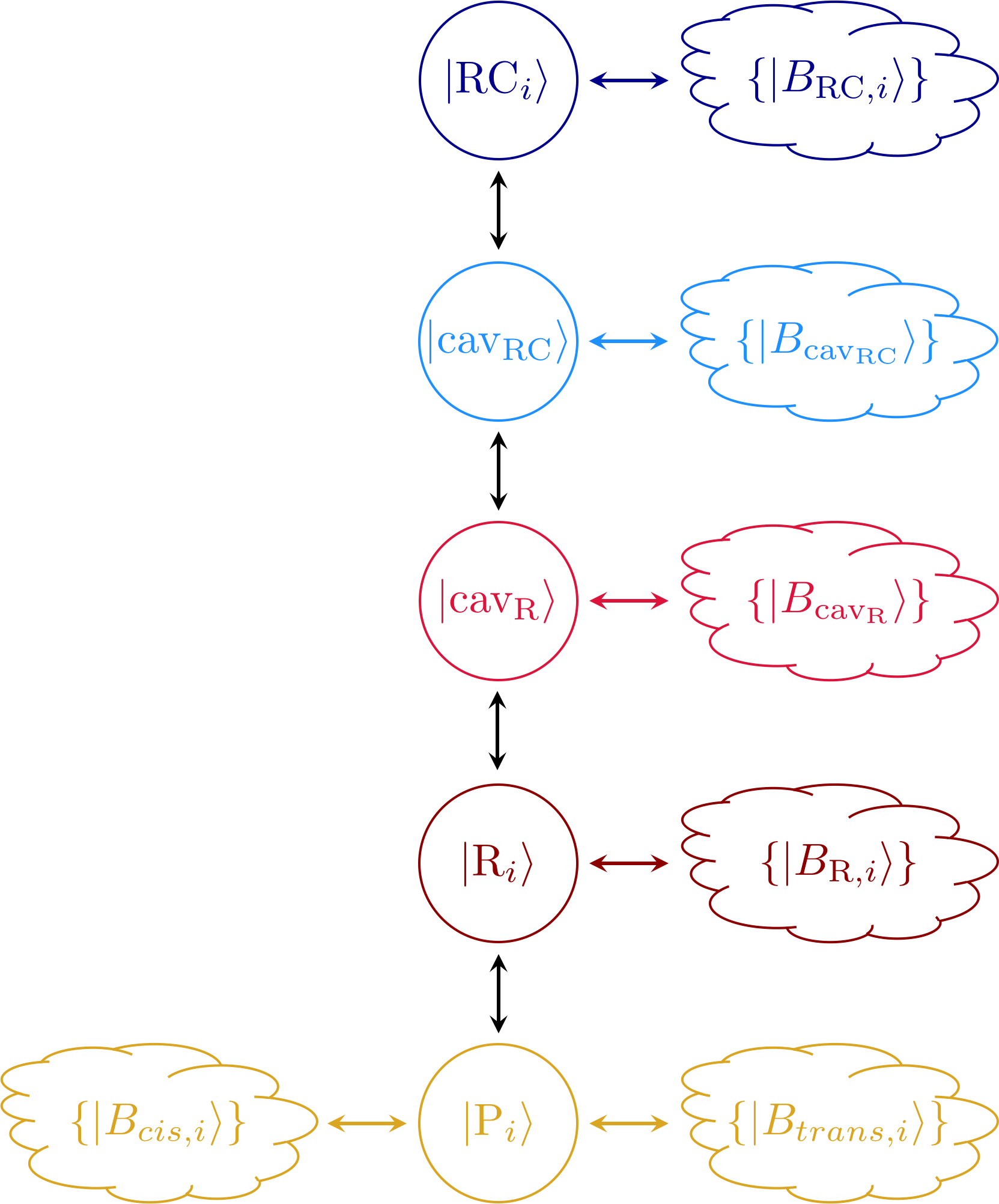
Supplementary Figure 2: Schematic of the system-bath interactions of the R $\rightarrow$ P fast isomerization channel for the polaritonic device. See equations (3), (S30), and those defining the terms therein, for Hamiltonian $H$. The $i$th molecule of compound $x=\text{RC},\text{R}$ has an OH stretch excitation $|x_{i}\rangle$ (dark blue, dark red circle), which is coupled to a set ${|B_{x}\rangle}$ of nonradiative bath states (dark blue, dark red clouds) that contributes to its decay. $|x_{i}\rangle$ is also coupled to photon $|\text{cav}_{x}\rangle$ of the cavity containing compound $x$. $|\text{cav}_{x}\rangle$ interacts with a set ${|B_{\text{cav}_{x}}\rangle}$ of radiative bath states, as well as with the other cavity state. For probe excitation of the polaritonic device, the states in ${|B_{\text{cav}_{\text{RC}}}\rangle}$ (light blue cloud) contribute to decay—in the form of transmission—of $|\text{cav}_{\text{R}C}\rangle$ (light blue circle), while the states in ${|B_{\text{cav}_{\text{R}}}\rangle}$ (light red cloud) contribute to decay—in the form of reflection—and excitation of $|\text{cav}_{\text{R}}\rangle$ (light red circle). Finally, $|\text{R}_{i}\rangle$ is coupled to another state, the torsional overtone $|\text{P}_{i}\rangle$ (yellow), which can concomitantly decay into either the $cis$ or $trans$ potential wells of HONO via coupling to ${|B_{cis,i}\rangle}$ or ${|B_{trans,i}\rangle}$, respectively.

As discussed in Methods, the Hamiltonian for the polaritonic device is $H=H_{\text{system}}+H_{\text{bath}}+H_{\text{system}-\text{bath}}$. The first term on the right-hand side is given by equation (3), as well as equation (4) in Methods. The latter two terms read

$$H_{\text{bath}} =\sum_{x=\text{RC},\,\text{cav}_{\text{RC}},\,\text{cav}_{\text{R}},\,\text{R},\,\text{P}}H_{\text{bath},x},$$ (S30a)

$$H_{\text{system}-\text{bath}} =\sum_{x=\text{RC},\,\text{cav}_{\text{RC}},\,\text{cav}_{\text{R}},\,\text{R},\,\text{P}}H_{\text{system}-\text{bath},x}.$$ (S30b)

In particular,

$$H_{\text{bath},x} =\sum_{i=1}^{N_{x}}\int_{-\infty}^{\infty}d\omega\,\omega B_{x,i}^{\dagger}(\omega)B_{x,i}(\omega),$$ (S31a)

$$H_{\text{bath},\text{cav}_{x}} =\int_{-\infty}^{\infty}d\omega\,\omega B_{\text{cav}_{x}}^{\dagger}(\omega)B_{\text{cav}_{x}}(\omega),$$ (S31b)

$$H_{\text{bath},\text{P}} =\sum_{y=cis,trans}\sum_{i=1}^{N_{\text{R}}}\int_{-\infty}^{\infty}d\omega\,\omega|B_{y,i}(\omega)\rangle\langle B_{y,i}(\omega)|,$$ (S31c)

and

$$H_{\text{system}-\text{bath},x} =\frac{\sqrt{\gamma_{x}}}{\sqrt{2\pi}}\sum_{i=1}^{N_{z}}\int_{-\infty}^{\infty}d\omega[a_{x,i}^{\dagger}B_{x,i}(\omega)+\text{h.c.}],$$ (S32a)

$$H_{\text{system}-\text{bath},\text{cav}_{x}} =\frac{\sqrt{\kappa_{x}}}{\sqrt{2\pi}}\int_{-\infty}^{\infty}d\omega[c_{x}^{\dagger}B_{\text{cav}_{x}}(\omega)+\text{h.c.}],$$ (S32b)

$$H_{\text{system}-\text{bath},\text{P}} =\sum_{y=cis,trans}\frac{\sqrt{\Gamma_{y}}}{\sqrt{2\pi}}\sum_{i=1}^{N_{\text{R}}}\int_{-\infty}^{\infty}d\omega[|\text{P}_{i}\rangle\langle B_{y,i}(\omega)|+\text{h.c.}]$$ (S32c)

for $x=\text{RC},\text{R}$. The various interactions between $|x_{i}\rangle=a_{x,i}^{\dagger}|\text{G}\rangle$, $|\text{cav}_{x}\rangle$, $|\text{P}_{i}\rangle$, and their baths are summarized in Fig. 2. In this Supplementary Note, $|\text{G}\rangle$ is the molecular and photonic vacuum ground state. The system-bath coupling parameters $\gamma_{x},\kappa_{x}$ are defined in Methods. Note that the bath modes for $|\text{R}\rangle$ only include the nonradiative degrees of freedom that induce its decay (cf. equations (S1b) and (S31a)). Since probe excitation of the polaritonic system would be carried out experimentally via laser impingement on the R cavity mirror, the radiative input is considered to couple only to the R cavity Ciuti and Carusotto (2006); Ribeiro et al. (2018b). The operators $a_{\text{RC},i}^{\dagger},a_{\text{RC},i}$ and $c_{x}^{\dagger},c_{x}$ for RC and the cavities, respectively, are defined in Methods. The operator $B_{\text{RC},i}^{\dagger}(\omega)$ ($B_{\text{RC},i}(\omega)$) creates (annihilates) an $|\text{RC}\rangle=\sum_{i=1}^{N_{\text{RC}}}|\text{RC}_{i}\rangle/\sqrt{N_{\text{RC}}}$ nonradiative bath mode of frequency $\omega$ on RC molecule $i$ and satisfies the bosonic commutation relations $[B_{\text{RC},i}(\omega),B_{\text{RC},i^{\prime}}^{\dagger}(\omega^{\prime})]=\delta_{i,i^{\prime}}\delta(\omega-\omega^{\prime})$ and $[B_{\text{RC},i}(\omega),B_{\text{RC},i^{\prime}}(\omega^{\prime})]=0$. Analogously, $B_{\text{cav}_{x}}^{\dagger}(\omega)$ ($B_{\text{cav}_{x}}(\omega)$) creates (annihilates) a $x$ cavity radiative bath mode of frequency $\omega$ and satisfies $[B_{\text{cav}_{x}}(\omega),B_{\text{cav}_{x}}^{\dagger}(\omega^{\prime})]=\delta(\omega-\omega^{\prime})$ and $[B_{\text{cav}_{x}}(\omega),B_{\text{cav}_{x}}(\omega^{\prime})]=0$.

To derive equations of motion for $|\text{RC}\rangle$, RC cavity, R cavity, $|\text{R}\rangle$, and $|\text{P}\rangle$, we first carry out standard input-output theory, specifically the steps taken in Supplementary Note 3 to obtain equations of motion (S15) and (S16) in the bare case. If we then account for the assumption made above that only the R cavity couples to an input field, we arrive at Heisenberg-Langevin equations (12a), (12c), (12d), (12e), and (12f), respectively, of Methods; in equation (12d), the term

$$c_{\text{R},\text{in}}(t)=\frac{i}{\sqrt{2\pi}}\int_{-\infty}^{\infty}d\omega B_{\text{cav}_{\text{R}}}(\omega)(t_{\text{in}})e^{-i\omega(t-t_{\text{in}})}$$ (S33)

is the R cavity input field that excites the R cavity at time $t_{\text{in}}$. Furthermore, applying this assumption and the steps invoked in 3 to obtain the bare input-output relations (equations (S12)-(S14)) yields the polaritonic input-output relations:

$$c_{\text{RC},\text{out}}(t) =\sqrt{\kappa_{\text{RC}}}c_{\text{RC}}(t),$$ (S34a)

$$c_{\text{R},\text{out}}(t)-c_{\text{R},\text{in}}(t) =\sqrt{\kappa_{\text{R}}}c_{\text{R}}(t),$$ (S34b)

$$P_{z,\text{out}}(t) =\sqrt{\gamma_{z}}P_{z}(t),$$ (S34c)

$$P_{\text{P},\text{out},y}(t) =\sqrt{\Gamma_{y}}P_{\text{P}}(t),$$ (S34d)

where

$$c_{x,\text{out}}(t) =\frac{i}{\sqrt{2\pi}}\int_{-\infty}^{\infty}d\omega B_{\text{cav}_{x}}(\omega)(t_{\text{out}})e^{-i\omega(t-t_{\text{out}})},$$ (S35)

$$P_{u,\text{out}}(t) =\frac{i}{\sqrt{2\pi}}\int_{-\infty}^{\infty}d\omega\beta_{u}(\omega)(t_{\text{out}})e^{-i\omega(t-t_{\text{out}})}$$ (S36)

annihilate output fields produced as energy is dissipated from the polaritonic system by bath modes at time $t_{\text{out}}>t$, and the different $\beta_{u}$ are defined as $\beta_{u}(\omega)=\sum_{i=1}^{N_{u}}B_{u,i}(\omega)/\sqrt{N_{u}}$ for $u=\text{R},\text{RC}$ and $\beta_{u}(\omega)=\sum_{i=1}^{N_{\text{R}}}|\text{G}\rangle\langle B_{u,i}(\omega)|/\sqrt{N_{\text{R}}}$ for $u=cis,trans$. Notice that for $|\text{P}\rangle$, the Heisenberg-Langevin equations (cf. equations (12f) and (S18)), input-output relations (cf. equations (S34d) and (S14)), and the associated notation are identical to those in the bare case (Supplementary Note 3). In contrast, the Heisenberg-Langevin equation (12a) contains the third-order RC polarization $P_{\text{RC},3}$ (defined in Methods), whose dynamics become relevant when the polaritonic device is pump-excited.

We now treat the dynamics of $P_{\text{RC},3}$, beginning with evaluation of the exact Heisenberg-Langevin equation for $a_{\text{RC},i}^{\dagger}a_{\text{RC},i}a_{\text{RC},i}$:

$$\frac{d[a_{\text{RC},i}^{\dagger}(t)a_{\text{RC},i}(t)a_{\text{RC},i}(t)]}{dt} =\frac{da_{\text{RC},i}^{\dagger}(t)}{dt}a_{\text{RC},i}(t)a_{\text{RC},i}(t)+a_{\text{RC},i}^{\dagger}(t)\frac{da_{\text{RC},i}(t)}{dt}a_{\text{RC},i}(t)+a_{\text{RC},i}^{\dagger}(t)a_{\text{RC},i}(t)\frac{da_{\text{RC},i}(t)}{dt}$$ (S37a)

$$=-i(\omega_{\text{RC}}-i3\gamma_{\text{RC}}/2+2\Delta)[a_{\text{RC},i}^{\dagger}(t)a_{\text{RC},i}(t)]a_{\text{RC},i}(t)-2ig_{\text{RC}}[a_{\text{RC},i}^{\dagger}(t)a_{\text{RC},i}(t)]c_{\text{RC}}(t)$$ (S37b)

$$\quad+ig_{\text{RC}}[c_{\text{RC}}^{\dagger}(t)a_{\text{RC},i}(t)]a_{\text{RC},j}(t)-2i\Delta[a_{\text{RC},i}^{\dagger}(t)a_{\text{RC},i}^{\dagger}(t)a_{\text{RC},i}(t)a_{\text{RC},i}(t)]a_{\text{RC},i}(t),$$ (S37c)

where in going from equations (S37a) to (S37b) and (S37c) we have used

$$\frac{da_{\text{RC},i}(t)}{dt}=-i(\omega_{\text{RC}}-i\gamma_{\text{RC}}/2)a_{\text{RC},i}(t)-ig_{\text{RC}}c_{\text{RC}}(t)-2i\Delta a_{\text{RC},i}^{\dagger}(t)a_{\text{RC},i}(t)a_{\text{RC},i}(t),$$ (S38)

obtainable by inspection of equation (12a). We now analyze the terms that contribute to the dynamics of the anharmonic-induced polarization. As written above, all terms in equation (S37b) and (S37c) are proportional to the product of a quantity in square brackets and a creation operator. In particular, the first (second) term in equation (S37b) is proportional to $[a_{\text{RC},i}^{\dagger}a_{\text{RC},i}]a_{\text{RC},i}$ ($[a_{\text{RC},i}^{\dagger}a_{\text{RC},i}]c_{\text{RC}}$) and interpretable as creation of a population in the first excited RC state followed by an RC (RC cavity) transition. On the other hand, the first (second) term in equation (S37c) is proportional to $[c_{\text{RC}}^{\dagger}a_{\text{RC},i}]a_{\text{RC},i}$ ($[a_{\text{RC},i}^{\dagger}a_{\text{RC},i}^{\dagger}a_{\text{RC},i}a_{\text{RC},i}]a_{\text{RC},i}$) and interpretable as the creation of a RC-cavity coherence (population of the second excited RC state) followed by an RC transition. Because we supposed that the pump pulse only creates singly excited RC population (in the form of dark RC states; see main text), we neglect both terms in equation (S37c) Ribeiro et al. (2018b). Moreover, we approximate the $a_{\text{RC},i}^{\dagger}a_{\text{RC},i}$ in the rightmost term of equation (S37b) as $f_{\text{pump}}=\sum_{i=1}^{N_{\text{RC}}}a_{\text{RC},i}^{\dagger}a_{\text{RC},i}/N_{\text{RC}}$, the effective fraction of total RC molecules populated via relaxation from polariton to RC dark states during the delay time Ribeiro et al. (2018b). With these steps, equation (S37) becomes equation (12b) in Methods.

We associate absorbance into RC, absorbance into R, and reaction efficiency $\eta$ with the fraction of the initial energy that is dissipated by the nonradiative bath of $|\text{RC}\rangle$, nonradiative bath of $|\text{R}\rangle$, and the bath inducing relaxation from $|\text{P}\rangle$ into the $trans$-HONO well, respectively. In analogy to using input-output equations (S13) and (S14) to obtain equations (S23) for R absorption and (S24) for reaction efficiency $\eta_{0}$ in the bare case, we employ polaritonic input-output equations (S34c) and (S34d) to write

$$\text{absorbance}_{\text{RC}}(f_{\text{pump}},\omega) =\gamma_{\text{R}}|S_{\text{RC}}(f_{\text{pump}},\omega)|^{2}$$ (S39)

$$\text{absorbance}_{\text{R}}(f_{\text{pump}},\omega) =\gamma_{\text{R}}|S_{\text{R}}(f_{\text{pump}},\omega)|^{2}$$ (S40)

$$\eta(f_{\text{pump}},\omega) =\Gamma_{trans}|S_{\text{P}}(f_{\text{pump}},\omega)|^{2}.$$ (S41)

The linear response functions $S_{\text{RC}}$, $S_{\text{R}}$, and $S_{\text{P}}$ are defined such that each multiplied by $c_{\text{R},\text{in}}(\omega)$ yields $P_{\text{RC}}(\omega)$, $P_{\text{R}}(\omega)$, and $P_{\text{P}}(\omega)$, respectively. From the Heisenberg-Langevin equations (12), it is evident that calculation of equations (S39)-(S41) requires knowledge of $V_{\text{R}-\text{P}}$. As we do in Supplementary Note 3 for the bare case, we perturbatively treat the IVR coupling in this Supplementary Note and neglect the terms containing $V_{\text{R}-\text{P}}$ in equations (S39) and (S40) for polaritonic spectra. The validity of this treatment can be shown by noticing that

$$P_{\text{R}}(\omega)=\frac{g_{\text{R}}\sqrt{N_{\text{R}}}[\omega-\omega_{\text{P}}+i(\Gamma_{cis}+\Gamma_{trans})/2]}{(\omega-\omega_{\text{R}}+i\gamma_{\text{nonrad}}/2)[\omega-\omega_{\text{P}}+i(\Gamma_{cis}+\Gamma_{trans})/2]-V_{\text{R}-\text{P}}^{2}}c_{\text{R}}(\omega),$$ (S42)

recognizing that the fraction on the right-hand side is equal to $S_{\text{R},0}(\omega)$ (equation (S21)) up to a constant, and analyzing the roots of the denominator of this fraction as done in the last paragraph of Supplementary Note 3.

Calculation of linear absorption spectra upon pumping the RC can be calculated in a fashion similar to equation (S34). There are two major procedural differences, which both arise in the Heisenberg-Langevin equations (12). For one, $f_{\text{pump}}$ is set to 0, and thus equation (12b) for the third-order polarization of RC can be neglected. Second, the only nonvanishing input operator is that of the RC cavity, not the R cavity. This change corresponds to dropping $c_{\text{R},\text{in}}$ in the Heisenberg-Langevin equation (12d) for the R cavity and adding

$$c_{\text{RC},\text{in}}(t)=\frac{i}{\sqrt{2\pi}}\int_{-\infty}^{\infty}d\omega B_{\text{cav}_{\text{RC}}}(\omega)(t_{\text{in}})e^{-i\omega(t-t_{\text{in}})}$$ (S43)

to the right-hand side of the corresponding equation (12c) for the RC cavity. Energy absorption of the pump pulse into R and RC is still calculated via equations (S40) and (S39), respectively, and is plotted in Fig. (3) for excitation of the highest polariton.

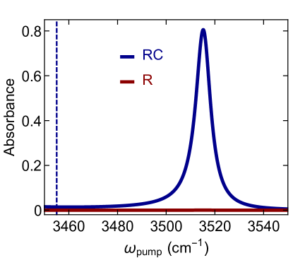
Supplementary Figure 3: Linear absorption of pump pulse due to RC and R. Spectra of energy absorption into RC and R upon excitation of the highest polariton (Supplementary Fig. 4b) with a pump pulse impinging on the mirror of the RC cavity (Fig. 1b). The dashed line indicates the energy of the bare OH stretch of RC (in the absence of strong light-matter coupling). Accounting for the lineshape broadening of the dark RC states and assuming this broadening is equal to that ($\gamma_{\text{RC}}$, see Methods) of the bare RC Du et al. (2018), there should exist bath degrees of freedom that mediate relaxation from the highest polariton to the dark RC states in a matrix of Kr, whose Debye frequency is $\sim 50\text{ cm}^{-1}$ Kittel (2004).

5 Derivation of pump-dependent effective Hamiltonian for polaritonic device

In this Supplementary Note, we outline the derivation for the pump-dependent effective Hamiltonian $H_{\text{system}}^{(\text{pump})}$ (equation (2)) for the polaritonic device. Although this Hamiltonian was not used for calculations of absorption and reaction efficiency, it provides an intuitive understanding of the associated Heisenberg-Langevin equation (12), on which these calculations are based as described in Methods. Precisely, $H_{\text{system}}^{(\text{pump})}$ describes the projection of the Heisenberg-Langevin equation on the system states, i.e., those acted on by $H_{\text{system}}$ (equation (3)), in the perturbative limit of $H_{\text{R}-\text{P}}$ (see equation (3)).

For reference, here we reproduce equation (12) disregarding $dP_{\text{P}}/dt$ and terms with $V_{\text{R}-\text{P}}$ and bath operator $c_{\text{R},\text{in}}(t)$ (equation (S33)):

$$\frac{dP_{\text{RC}}(t)}{dt} =-i(\omega_{\text{RC}}-i\gamma_{\text{RC}}/2)P_{\text{RC}}(t)$$

$$\quad-ig_{\text{RC}}\sqrt{N_{\text{RC}}}c_{\text{RC}}(t)-2i\Delta P_{\text{RC},3}(t),$$ (S44)

$$\frac{dP_{\text{RC},3}(t)}{dt} =-i(\omega_{\text{RC}}+2\Delta-i3\gamma_{\text{RC}}/2)P_{\text{RC},3}(t)$$

$$\quad-2ig_{\text{RC}}f_{\text{pump}}\sqrt{N_{\text{RC}}}c_{\text{RC}}(t),$$ (S45)

$$\frac{dc_{\text{RC}}(t)}{dt} =-i(\omega_{\text{cav}_{\text{RC}}}-i\kappa_{\text{RC}}/2)c_{\text{RC}}(t)$$

$$\quad-ig_{\text{cav}}c_{\text{R}}(t)-ig_{\text{RC}}\sqrt{N_{\text{RC}}}P_{\text{RC}}(t),$$ (S46)

$$\frac{dc_{\text{R}}(t)}{dt} =-i(\omega_{\text{cav}_{\text{R}}}-i\kappa_{\text{R}}/2)c_{\text{R}}(t)-ig_{\text{cav}}c_{\text{RC}}(t)$$

$$\quad-ig_{\text{R}}\sqrt{N_{\text{R}}}P_{\text{R}}(t),$$ (S47)

$$\frac{dP_{\text{R}}(t)}{dt} =-i(\omega_{\text{R}}-i\gamma_{\text{R}}/2)P_{\text{R}}(t)$$

$$\quad-ig_{\text{R}}\sqrt{N_{\text{R}}}c_{\text{R}}(t).$$ (S48)

Define

$$P_{\text{RC}}^{\prime} =\frac{P_{\text{RC}}-P_{\text{RC},3}}{\sqrt{(1-2f_{\text{pump}})}}$$ (S49a)

$$=\frac{\sum_{i=1}^{N_{\text{RC}}}(1-a_{i}^{\dagger}a_{i})a_{i}}{\sqrt{(1-2f_{\text{pump}})N_{\text{RC}}}}$$ (S49b)

and

$$P_{\text{RC},3}^{\prime} =\frac{P_{\text{RC},3}}{\sqrt{2f_{\text{pump}}}}$$ (S50a)

$$=\frac{\sum_{i=1}^{N_{\text{RC}}}(a_{i}^{\dagger}a_{i})a_{i}}{\sqrt{2f_{\text{pump}}N_{\text{RC}}}}.$$ (S50b)

It is possible to check that

$$i\partial_{t}\vec{v}=[H_{\text{system}}^{(\text{pump})}+H_{\text{system}}^{(\text{pump}),\text{non-Hermitian}}]\vec{v},$$ (S51)

where $\vec{v}=(P_{\text{RC}}^{\prime},P_{\text{RC},3}^{\prime},c_{\text{RC}},c_{\text{R}},P_{\text{R}})$, and $H_{\text{system}}^{(\text{pump})}$ and $H_{\text{system}}^{(\text{pump}),\text{non-Hermitian}}$ are respectively Hermitian and non-Hermitian parts,

$$H_{\text{system}}^{(\text{pump})} =\begin{pmatrix}\omega_{\text{RC}}&0&g_{\text{RC}}\sqrt{(1-2f_{\text{pump}})N_{\text{RC}}}&0&0\\ 0&\omega_{\text{RC}}+2\Delta&g_{\text{RC}}\sqrt{2f_{\text{pump}}N_{\text{RC}}}&0&0\\ g_{\text{RC}}\sqrt{(1-2f_{\text{pump}})N_{\text{RC}}}&g_{\text{RC}}\sqrt{2f_{\text{pump}}N_{\text{RC}}}&\omega_{\text{cav}_{\text{RC}}}&g_{\text{cav}}&0\\ 0&0&g_{\text{cav}}&\omega_{\text{cav}_{\text{R}}}&g_{\text{R}}\sqrt{N_{\text{R}}}\\ 0&0&0&g_{\text{R}}\sqrt{N_{\text{R}}}&\omega_{\text{R}}\end{pmatrix},$$ (S52)

$$H_{\text{system}}^{(\text{pump}),\text{non-Hermitian}} =\begin{pmatrix}-i\gamma_{\text{RC}}/2&i\gamma_{\text{RC}}\sqrt{2f_{\text{pump}}/(1-2f_{\text{pump}})}&0&0&0\\ 0&-i3\gamma_{\text{RC}}/2&0&0&0\\ 0&0&-i\kappa_{\text{RC}}/2&0&0\\ 0&0&0&-i\kappa_{\text{R}}/2&0\\ 0&0&0&0&-i\gamma_{\text{R}}/2\end{pmatrix}.$$ (S53)

Since only $H_{\text{system}}^{(\text{pump})}$ depends on parameters of $H_{\text{system}}$, while only $H_{\text{system}}^{(\text{pump}),\text{non-Hermitian}}$ depends on dissipative parameters$\gamma_{x},\kappa_{x}$ for $x=\text{R},\text{RC}$, equation (S51) provides the appealing effective physical interpretation that $H_{\text{system}}^{(\text{pump})}$ governs the coherent dynamics of the pumped system while $H_{\text{system}}^{(\text{pump}),\text{non-Hermitian}}$ characterizes its losses. In particular, we deduce Ribeiro et al. (2018b) that $P_{\text{RC}}^{\prime}$ represents the 0 $\rightarrow$ 1 $|\text{RC}\rangle$ transition whose light-matter coupling reflects the combined amplitudes of ground-state absorption and stimulated emission, whereas $P_{\text{RC},3}^{\prime}$ represents the 1 $\rightarrow$ 2 $|\text{RC}\rangle$ transition whose light-matter coupling reflects the amplitudes of excited-state absorption. Although this interpretation was heuristically obtained in previous work Ribeiro et al. (2018b), equations (S49) and (S50) provide a formal justification for it. Additionally, all other results in this work that follow from $H_{\text{system}}^{(\text{pump})}$—including Figs. 2 and 4 and associated discussion—are for qualitative understanding only, precluding the need to ever specify which of $P_{\text{RC}}$ or $P_{\text{RC}}^{\prime}$ ($P_{\text{RC},3}$ or $P_{\text{RC},3}^{\prime}$) these results pertain when referring to the 0 $\rightarrow$ 1 (1 $\rightarrow$ 2) $|\text{RC}\rangle$ transition.

6 Representations of mixing fractions and energies for polaritonic device

In Supplementary Fig. 4, the plotted polariton mixing fractions and energies are determined by diagonalization of system Hamiltonian $H_{\text{system}}^{(\text{no pump})}$ (equation (1)) for no pumping (a,b) or effective Hamiltonian $H_{\text{system}}^{(\text{pump})}$ (equation (2), see Supplementary Note 5 for derivation and interpretation) for pumping (c).

In Fig. 2, color gradients and vertical positions of the polariton line segments represent the mixing fractions and relative energies, respectively, from Supplementary Fig. 4. Specifically, [a, red and blue panels], [a, purple panel, and b, left panel], and [b, right panel] of the former figure correspond respectively to a, b, and c of the latter. To produce the (continuum) color gradients in Fig. 2, we use the following algorithms to create significant resemblance to the discrete color gradients in Fig. 4.

First consider the case without pumping. Denote the mixing fraction of species $i=1,2,3,4$—corresponding to $|\text{cav}_{\text{RC}}\rangle,|\text{RC}\rangle,|\text{R}\rangle,|\text{cav}_{\text{R}}\rangle$, respectively—for polariton $n=1,2,3,4$ as $f_{x}^{(i)}$, where the polaritons are indexed from highest energy ($i=1$) to lowest energy ($i=4$), and $\sum_{i}f_{i}^{(n)}=\sum_{n}f_{i}^{(n)}=1$. Then we define quantities $g_{i}^{(n)}$ to indicate the positions of gradient markers for polariton $i$ and species $x$:

$$g_{i}^{(n)}=\begin{cases}\text{round}\left(100\times(f_{i}^{(n)}+f_{i+1}^{(n)})/2\right)&i=1,2,3\\ \text{round}\left((100\times(f_{i}^{(n)}+1)/2)\right)&i=4\end{cases}$$

where $\text{round}(x)=\lceil x-0.5\rceil$ maps $x\in\mathbb{R}$ to the nearest integer (and odd multiples of 0.5 to the lower of the two equally close nearest integers). For each $n$ and a gradient scale that ranges from 0-100, a marker is at position $g_{i}^{(n)}\neq 0$ with the color assigned to species $i$; if $g_{i}^{(n)}=0$, no marker is placed.

The case with pumping is similar. Due to the large anharmonicity of $|\text{RC}\rangle$, the lowest-energy eigenstate of the effective Hamiltonian equation (2) essentially represents just the $|\text{RC}\rangle$ 1 $\rightarrow$ 2 transition. The remaining eigenstates, which correspond to the polaritons, have insignificant character of this transition (Fig. 4c). We therefore combine the mixing fraction of the $|\text{RC}\rangle$ 1 $\rightarrow$ 2 transition with that of $|\text{RC}\rangle$. The gradient markers are then placed as described above for the case without pumping.

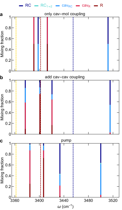
Supplementary Figure 4: Effects of strong coupling and pumping on hybridization. The eigenstates and mixing fractions of the polaritonic device (Fig. 1) under different circumstances for parameters used in the simulations of Fig. 3: a, with strong coupling between each cavity and the 0 $\rightarrow$ 1 OH stretches of its hosted molecules, b, with cavity-molecule and cavity-cavity strong coupling, and c, after a pump pulse acting on the system described by b excites 30% of RC molecules into the $v=1$ OH state. In each plot, the dashed lines indicate the bare energies of the 0 $\rightarrow$ 1 vibrational transitions of RC (dark blue) and reactant (R, dark red), as well as that of the quantum state $|\text{P}\rangle$ (yellow) that first receives population from $|\text{R}\rangle$ via IVR and then relaxes into P states (see main text).

References

- Törmä and Barnes (2015) P. Törmä and W. L. Barnes, Rep. Prog. Phys. 78, 013901 (2015).
- Agranovich et al. (2011) V. M. Agranovich, Y. N. Gartstein, and M. Litinskaya, Chem. Rev. 111, 5179 (2011).
- Neuman and Aizpurua (2018) T. Neuman and J. Aizpurua, arXiv preprint arXiv:1804.08878 (2018).
- Ebbesen (2016) T. W. Ebbesen, Acc. Chem. Res. 49, 2403 (2016).
- Ribeiro et al. (2018a) R. F. Ribeiro, L. A. Martínez-Martínez, M. Du, J. Campos-Gonzalez-Angulo, and J. Yuen-Zhou, Chem. Sci. 9, 6325 (2018a).
- Feist et al. (2017) J. Feist, J. Galego, and F. J. Garcia-Vidal, ACS Photonics 5, 205 (2017).
- Flick et al. (2018) J. Flick, N. Rivera, and P. Narang, Nanophotonics 7, 1479 (2018).
- Schäfer et al. (2018) C. Schäfer, M. Ruggenthaler, and A. Rubio, Phys. Rev. A 98, 043801 (2018).
- Hutchison et al. (2012) J. A. Hutchison, T. Schwartz, C. Genet, E. Devaux, and T. W. Ebbesen, Angew. Chem., Int. Ed. 51, 1592 (2012).
- Stranius et al. (2018) K. Stranius, M. Hertzog, and K. Börjesson, Nat. Commun. 9, 2273 (2018).
- Munkhbat et al. (2018) B. Munkhbat, M. Wersäll, D. G. Baranov, T. J. Antosiewicz, and T. Shegai, Sci. Adv. 4 (2018).
- Polak et al. (2018) D. Polak, R. Jayaprakash, A. Leventis, K. J. Fallon, H. Coulthard, A. J. Petty, II, J. Anthony, H. Bronstein, D. G. Lidzey, J. Clark, and A. J. Musser, arXiv preprint arXiv:1806.09990 (2018).
- Shi et al. (2018) X. Shi, K. Ueno, T. Oshikiri, Q. Sun, K. Sasaki, and H. Misawa, Nat. Nanotechnol. 13, 953 (2018).
- Herrera and Spano (2016) F. Herrera and F. C. Spano, Phys. Rev. Lett. 116, 238301 (2016).
- Groenhof and Toppari (2018) G. Groenhof and J. J. Toppari, J. Phys. Chem. Lett. , 4848 (2018).
- Kowalewski et al. (2016) M. Kowalewski, K. Bennett, and S. Mukamel, J. Phys. Chem. Lett. 7, 2050 (2016).
- Vendrell (2018) O. Vendrell, Chem. Phys. 509, 55 (2018).
- Galego et al. (2016) J. Galego, F. J. Garcia-Vidal, and J. Feist, Nat. Commun. 7, 13841 (2016).
- Martínez-Martínez et al. (2018) L. A. Martínez-Martínez, M. Du, R. F. Ribeiro, S. Kéna-Cohen, and J. Yuen-Zhou, J. Phys. Chem. Lett. 9, 1951 (2018).
- Zhong et al. (2017) X. Zhong, T. Chervy, L. Zhang, A. Thomas, J. George, C. Genet, J. A. Hutchison, and T. W. Ebbesen, Angew. Chem., Int. Ed. 56, 9034 (2017).
- Du et al. (2018) M. Du, L. A. Martínez-Martínez, R. F. Ribeiro, Z. Hu, V. M. Menon, and J. Yuen-Zhou, Chem. Sci. 9, 6659 (2018).
- Sáez-Blázquez et al. (2018) R. Sáez-Blázquez, J. Feist, A. I. Fernández-Domínguez, and F. J. García-Vidal, Phys. Rev. B 97, 241407 (2018).
- Reitz et al. (2018) M. Reitz, F. Mineo, and C. Genes, Sci. Rep. 8, 9050 (2018).
- Schachenmayer et al. (2015) J. Schachenmayer, C. Genes, E. Tignone, and G. Pupillo, Phys. Rev. Lett. 114, 196403 (2015).
- Dunkelberger et al. (2016) A. D. Dunkelberger, B. T. Spann, K. P. Fears, B. S. Simpkins, and J. C. Owrutsky, Nat. Commun. 7, 13504 (2016).
- Dunkelberger et al. (2018) A. D. Dunkelberger, R. B. Davidson II, W. Ahn, B. S. Simpkins, and J. C. Owrutsky, J. Phys. Chem. A 122, 965 (2018).
- Xiang et al. (2018) B. Xiang, R. F. Ribeiro, A. D. Dunkelberger, J. Wang, Y. Li, B. S. Simpkins, J. C. Owrutsky, J. Yuen-Zhou, and W. Xiong, Proc. Natl. Acad. Sci. U. S. A. 115, 4845 (2018).
- Ribeiro et al. (2018b) R. F. Ribeiro, A. D. Dunkelberger, B. Xiang, W. Xiong, B. S. Simpkins, J. C. Owrutsky, and J. Yuen-Zhou, J. Phys. Chem. Lett. 9, 3766 (2018b).
- del Pino et al. (2015) J. del Pino, J. Feist, and F. J. Garcia-Vidal, New J. Phys. 17, 053040 (2015).
- Schanz et al. (2005) R. Schanz, V. Boţan, and P. Hamm, J. Chem. Phys. 122, 044509 (2005).
- Olbert-Majkut et al. (2014a) A. Olbert-Majkut, M. Wierzejewska, and J. Lundell, Chem. Phys. Lett. 616-617, 91 (2014a).
- Olbert-Majkut et al. (2014b) A. Olbert-Majkut, J. Lundell, and M. Wierzejewska, J. Phys. Chem. A 118, 350 (2014b).
- Stanley et al. (1994) R. P. Stanley, R. Houdré, U. Oesterle, M. Ilegems, and C. Weisbuch, Appl. Phys. Lett. 65, 2093 (1994).
- Nesbitt and Field (1996) D. J. Nesbitt and R. W. Field, J. Phys. Chem. 100, 12735 (1996).
- Hall and Pimentel (1963) R. T. Hall and G. C. Pimentel, J. Chem. Phys. 38, 1889 (1963).
- Gardiner and Collett (1985) C. W. Gardiner and M. J. Collett, Phys. Rev. A 31, 3761 (1985).
- Ciuti and Carusotto (2006) C. Ciuti and I. Carusotto, Phys. Rev. A 74, 033811 (2006).
- Li et al. (2017) H. Li, A. Piryatinski, J. Jerke, A. R. S. Kandada, C. Silva, and E. R. Bittner, Quantum Sci. Technol. 3, 015003 (2017).
- Ćwik et al. (2016) J. A. Ćwik, P. Kirton, S. De Liberato, and J. Keeling, Phys. Rev. A 93, 033840 (2016).
- Szidarovszky et al. (2018) T. Szidarovszky, G. J. Halász, A. G. Császár, L. S. Cederbaum, and A. Vibók, J. Phys. Chem. Lett. , 6215 (2018).
- Casey and Sparks (2016) S. R. Casey and J. R. Sparks, J. Phys. Chem. C 120, 28138 (2016).
- Skolnick et al. (1998) M. S. Skolnick, T. A. Fisher, and D. M. Whittaker, Semicond. Sci. Technol. 13, 645 (1998).
- Khitrova et al. (1999) G. Khitrova, H. M. Gibbs, F. Jahnke, M. Kira, and S. W. Koch, Rev. Mod. Phys. 71, 1591 (1999).
- Vasa et al. (2013) P. Vasa, W. Wang, R. Pomraenke, M. Lammers, M. Maiuri, C. Manzoni, G. Cerullo, and C. Lienau, Nat. Photonics 7, 128 (2013).
- Liu et al. (2015) B. Liu, P. Rai, J. Grezmak, R. J. Twieg, and K. D. Singer, Phys. Rev. B 92, 155301 (2015).
- Bellessa et al. (2004) J. Bellessa, C. Bonnand, J. C. Plenet, and J. Mugnier, Phys. Rev. Lett. 93, 036404 (2004).
- Maxim and Abraham (2017) S. Maxim and N. Abraham, J. Phys.: Condens. Matter 29, 443003 (2017).
- Fofang et al. (2011) N. T. Fofang, N. K. Grady, Z. Fan, A. O. Govorov, and N. J. Halas, Nano Lett. 11, 1556 (2011).
- Prodan et al. (2003) E. Prodan, C. Radloff, N. J. Halas, and P. Nordlander, Science 302, 419 (2003).
- Thakkar et al. (2017) N. Thakkar, M. T. Rea, K. C. Smith, K. D. Heylman, S. C. Quillin, K. A. Knapper, E. H. Horak, D. J. Masiello, and R. H. Goldsmith, Nano Lett. 17, 6927 (2017).
- Shapiro and Brumer (2012) M. Shapiro and P. Brumer, Quantum Control of Molecular Processes (Wiley, 2012).
- Hamm (2008) P. Hamm, Chem. Phys. 347, 503 (2008).
- Steck (2007) D. A. Steck, Quantum and atom optics, Vol. 47 (Oregon Center for Optics and Department of Physics, University of Oregon, Eugene, Oregon, 2007).
- Nitzan (2006) A. Nitzan, Chemical Dynamics in Condensed Phases: Relaxation, Transfer and Reactions in Condensed Molecular Systems (OUP Oxford, 2006).
- Segal and Nitzan (2001) D. Segal and A. Nitzan, Chem. Phys. 268, 315 (2001).
- Khriachtchev et al. (2000) L. Khriachtchev, J. Lundell, E. Isoniemi, and M. Räsänen, J. Chem. Phys. 113, 4265 (2000).
- Kittel (2004) C. Kittel, Introduction to Solid State Physics (Wiley, 2004).