Model Selection for Nonnegative Matrix Factorization by Support Union Recovery

Abstract

Nonnegative matrix factorization (NMF) has been widely used in machine learning and signal processing because of its non-subtractive, part-based property which enhances interpretability. It is often assumed that the latent dimensionality (or the number of components) is given. Despite the large amount of algorithms designed for NMF, there is little literature about automatic model selection for NMF with theoretical guarantees. In this paper, we propose an algorithm that first calculates an empirical second-order moment from the empirical fourth-order cumulant tensor, and then estimates the latent dimensionality by recovering the support union (the index set of non-zero rows) of a matrix related to the empirical second-order moment. By assuming a generative model of the data with additional mild conditions, our algorithm provably detects the true latent dimensionality. We show on synthetic examples that our proposed algorithm is able to find an approximately correct number of components.

I Introduction

In a nonnegative matrix factorization (NMF) problem, we are given a data matrix $\mathbf{V}\in\mathbb{R}^{F\times N}$, and we seek non-negative factor matrices $\mathbf{W}\in\mathbb{R}^{F\times K}$, $\mathbf{H}\in\mathbb{R}^{K\times N}$ such that a certain distance between $\mathbf{V}$ and $\mathbf{W}\mathbf{H}$ is minimized. To reduce the data dimension and for the purpose of efficient computation, the integer $K$, which is said to be the latent dimensionality or the number of components, is usually chosen such that $K(F+N)\ll FN$. Since the publication of the seminar paper [1] in 2000, NMF has been a popular topic in machine learning [2] and signal processing [3]. There are many fundamental algorithms to approximately solve the NMF problem [1, 4, 5] with the implicit assumption that an effective number of the latent dimensionality is known a priori.

Despite the practical success of these fundamental algorithms, the estimation of the latent dimensionality remains an important issue. For example, researchers may wonder whether we can achieve better approximation accuracy with significantly less running time by selecting a better $K$ as the input of the algorithm. Unfortunately, there is generally little literature discussing the model selection problem for NMF. Moreover, the methods proposed in papers about detecting latent dimensionality for NMF [6, 7, 8, 9] either lack theoretical guarantees or require rather stringent conditions on the generative model of data.

I-A Main Contributions

We assume that each column $\mathbf{v}$ of the data matrix $\mathbf{V}=[\mathbf{v}_{1},\mathbf{v}_{2},\ldots,\mathbf{v}_{N}]\in\mathbb{R}^{F\times N}$ is sampled from the following generative model

$$\mathbf{v}=\mathbf{W}\mathbf{h}+\mathbf{z},$$ (1)

where $\mathbf{W}=[\mathbf{w}_{1},\mathbf{w}_{2},\ldots,\mathbf{w}_{K}]\in\mathbb{R}^{F\times K}_{+}$ is the mixing matrix (or the ground-truth non-negative dictionary matrix) and we assume that $\operatorname{rank}(\mathbf{W})=K$. $\mathbf{h}\in\mathbb{R}^{K}$ is a latent random vector with independent coordinates, and $\mathbf{z}\in\mathbb{R}^{F}$ is a multivariate Gaussian random vector. $\mathbf{z}$ is assumed to be independent with $\mathbf{h}$. We write $\mathbf{H}=[\mathbf{h}_{1},\mathbf{h}_{2},\ldots,\mathbf{h}_{N}]\in\mathbb{R}^{K\times N}$. In the context of this generative model, our goal is to find the number of columns of $\mathbf{W}$ from the observed matrix $\mathbf{V}$. This generative model can be viewed as a non-negative variant of that for independent component analysis (ICA) [11].

For the data matrix $\mathbf{V}\in\mathbb{R}^{F\times N}$ generated from the above model, we first calculate an empirical second-order moment, denoted as $\hat{\mathbf{M}}_{2}\in\mathbb{R}^{F\times F}$, from the empirical fourth-order cumulant tensor. We prove that $\hat{\mathbf{M}}_{2}$ approximates its expectation, denoted as $\mathbf{M}_{2}$, well with high probability when $N$ is sufficiently large. We also show that $\mathbf{M}_{2}$ can be written as $\mathbf{M}_{2}=\mathbf{M}_{2}\mathbf{X}^{*}$, where $\mathbf{X}^{*}\in\mathbb{R}^{F\times F}$ contains exactly $K$ non-zero rows. Finally, we prove that under certain conditions, an $\ell_{1}/\ell_{2}$ block norm minimization problem (cf. (63) to follow) over $\hat{\mathbf{M}}_{2}$ is able to detect the correct number of column of $\mathbf{W}$ from the recovery of a support union.

I-B Notations

We use capital boldface letters to denote matrices and we use lower-case boldface letters to denote vectors. We use $a_{ij}$ or $[\mathbf{A}]_{ij}$ to denote the $(i,j)$-th entry of $\mathbf{A}$. $\left[N\right]$ represents $\{1,2,\cdots,N\}$ for any positive integer $N$. For $\mathbf{X}\in\mathbb{R}^{L\times M}$ and any $l\in[L]$, $m\in[M]$, we use $\underline{\mathbf{x}}_{l}$, $\mathbf{x}_{m}$ to denote the $l$-th row and the $m$-th column of $\mathbf{X}$, respectively. We write $\underline{\mathbf{V}}_{\mathscr{K}}:=\mathbf{V}(\mathscr{K},\colon)$ as the rows of $\mathbf{V}$ indexed by $\mathscr{K}$, and $\mathbf{V}_{\mathscr{K}}:=\mathbf{V}\left(\colon,\mathscr{K}\right)$ denotes the columns of $\mathbf{V}$ indexed by $\mathscr{K}$. $\|\mathbf{V}\|_{1},\|\mathbf{V}\|_{2},\|\mathbf{V}\|_{\infty},\|\mathbf{V}\|_{\mathrm{F}}$ represents the $1$-norm, the spectral norm, the infinity norm and the Frobenius norm of $\mathbf{V}$, respectively. Let $\mathbf{V}_{1}\in\mathbb{R}^{F_{1}\times N}$ and $\mathbf{V}_{2}\in\mathbb{R}^{F_{2}\times N}$. We denote by $\left[\mathbf{V}_{1};\mathbf{V}_{2}\right]$ the vertical concatenation of the two matrices. $\mathrm{Diag}(\mathbf{w})$ represents the diagonal matrix whose diagonal entries are given by $\mathbf{w}$. The support of a vector $\mathbf{x}$ is denoted as $\mathrm{supp}(\mathbf{x}):=\{i:x_{i}\neq 0\}$. The support union of a matrix $\mathbf{X}$ with $N$ columns is defined as $\mathrm{Supp}(\mathbf{X}):=\cup_{n=1}^{N}\mathrm{supp}(\mathbf{x}_{n})$.

II Tensor Methods

In this section, we calculate an empirical second moment $\hat{\mathbf{M}}_{2}$ using a tensor method, and we prove that the empirical second moment is close to its expectation $\mathbf{M}_{2}$ with high probability when the sample size $N$ is sufficiently large.

II-A The Derivation of $\mathbf{M}_{2}$ and $\hat{\mathbf{M}}_{2}$

Let $\mathbf{v}$ be a random vector corresponding to the generative model (1) with $\mathbb{E}[h_{k}]=0$ and $\mathbb{E}[z_{f}]=0$ for $k\in[K],f\in[F]$. We have the following lemma which says that $\mathbf{M}_{2}$ can be written in a nice form.

Lemma 1 ([12, 13])

Define

$$\mathcal{M}_{4}:=\mathbb{E}[\mathbf{v}\otimes\mathbf{v}\otimes\mathbf{v}\otimes\mathbf{v}]-\mathcal{T},$$ (2)

where $[\mathbf{v}\otimes\mathbf{v}\otimes\mathbf{v}\otimes\mathbf{v}]_{ijlm}=v_{i}v_{j}v_{l}v_{m}$ and $\mathcal{T}$ is the fourth-order tensor with

$$[\mathcal{T}]_{ijlm} :=\mathbb{E}[v_{i}v_{j}]\mathbb{E}[v_{l}v_{m}]+\mathbb{E}[v_{i}v_{l}]\mathbb{E}[v_{j}v_{m}]$$

$$+\mathbb{E}[v_{i}v_{m}]\mathbb{E}[v_{j}v_{l}]$$ (3)

for all $i,j,l,m\in[F]$. Let $\kappa_{k}=\mathbb{E}[h_{k}^{4}]-3\mathbb{E}[h_{k}^{2}]$ for each $k\in[K]$. Then

$$\mathcal{M}_{4}=\sum_{k=1}^{K}\kappa_{k}\mathbf{w}_{k}\otimes\mathbf{w}_{k}\otimes\mathbf{w}_{k}\otimes\mathbf{w}_{k}.$$ (4)

In addition, we have that

$$\mathbf{M}_{2}:=\mathcal{M}_{4}(\mathbf{I},\mathbf{I},\mathbf{s},\mathbf{t})=\sum_{k=1}^{K}\kappa_{k}(\mathbf{s}^{T}\mathbf{w}_{k})(\mathbf{t}^{T}\mathbf{w}_{k})\mathbf{w}_{k}\otimes\mathbf{w}_{k}$$ (5)

for any $\mathbf{s},\mathbf{t}\in\mathbb{R}^{F}$. Here for matrices $\mathbf{V}_{1}\in\mathbb{R}^{F\times F_{1}},\mathbf{V}_{2}\in\mathbb{R}^{F\times F_{2}},\mathbf{V}_{3}\in\mathbb{R}^{F\times F_{3}},\mathbf{V}_{4}\in\mathbb{R}^{F\times F_{4}}$, $\mathcal{M}_{4}(\mathbf{V}_{1},\mathbf{V}_{2},\mathbf{V}_{3},\mathbf{V}_{4})$ is defined as the tensor whose $(i_{1},i_{2},i_{3},i_{4})$-th entry is

$$\left[\mathcal{M}_{4}(\mathbf{V}_{1},\mathbf{V}_{2},\mathbf{V}_{3},\mathbf{V}_{4})\right]_{i_{1},i_{2},i_{3},i_{4}}=$$

$$\sum_{j_{1},j_{2},j_{3},j_{4}}\left[\mathcal{M}_{4}\right]_{j_{1},j_{2},j_{3},j_{4}}[\mathbf{V}_{1}]_{j_{1},i_{1}}[\mathbf{V}_{2}]_{j_{2},i_{2}}[\mathbf{V}_{3}]_{j_{3},i_{3}}[\mathbf{V}_{4}]_{j_{4},i_{4}}.$$ (6)

We calculate $\hat{\mathbf{M}}_{2}$ from the sample matrix $\mathbf{V}$. Let

$$\hat{\mathcal{M}}_{4}:=\frac{\sum_{n=1}^{N}\mathbf{v}_{n}\otimes\mathbf{v}_{n}\otimes\mathbf{v}_{n}\otimes\mathbf{v}_{n}}{N}-\hat{\mathcal{T}},$$ (7)

where for $1\leq i,j,l,m\leq F$,

$$[\hat{\mathcal{T}}]_{ijlm}=\frac{\sum_{n=1}^{N}v_{i,n}v_{j,n}}{N}\frac{\sum_{n=1}^{N}v_{l,n}v_{m,n}}{N}+$$

$$\frac{\sum_{n=1}^{N}v_{i,n}v_{l,n}}{N}\frac{\sum_{n=1}^{N}v_{j,n}v_{m,n}}{N}+\frac{\sum_{n=1}^{N}v_{i,n}v_{m,n}}{N}\frac{\sum_{n=1}^{N}v_{j,n}v_{l,n}}{N}.$$ (8)

Denoting $\hat{\mathbf{M}}_{2}$ as

$$\hat{\mathbf{M}}_{2}=\hat{\mathcal{M}}_{4}(\mathbf{I},\mathbf{I},\mathbf{s},\mathbf{t}).$$ (9)

We have that $\mathbb{E}[\hat{\mathbf{M}}_{2}]=\mathbf{M}_{2}$. For simplicity, we take $\mathbf{s}=\mathbf{t}=\mathbf{e}\in\mathbb{R}^{F}$, where $\mathbf{e}$ is the vector of all ones. For any $k\in[K]$, because $\mathbf{w}_{k}\neq\mathbf{0}$, we have that $\mathbf{e}^{T}\mathbf{w}_{k}>0$. In addition, if $\kappa_{k}\neq 0$, let $\alpha_{k}=\kappa_{k}(\mathbf{e}^{T}\mathbf{w}_{k})^{2}$, we have $\alpha_{k}\neq 0$ and

$$\mathbf{M}_{2}=\sum_{k=1}^{K}\alpha_{k}\mathbf{w}_{k}\mathbf{w}_{k}^{T}.$$ (10)

Moreover, now we have that

$$[\hat{\mathbf{M}}_{2}]_{ij}=\sum_{l=1}^{F}\sum_{m=1}^{F}[\hat{\mathcal{M}}_{4}]_{ijlm}.$$ (11)

II-B Bounding the Distance between $\mathbf{M}_{2}$ and $\hat{\mathbf{M}}_{2}$

Let $\mathbf{E}=\hat{\mathbf{M}}_{2}-\mathbf{M}_{2}$, and assume that all the coordinates of $\mathbf{h}$ are identically and independently distributed with $m_{p}:=\mathbb{E}[h_{k}^{p}]$ for all $k\in[K]$, $p\in\mathbb{N}$. In particular, we assume that $m_{1}=0$ and $m_{4}\neq 3m_{2}$. Let $M_{8}=m_{8}+m_{7}m_{1}+m_{6}m_{2}+m_{6}m_{1}^{2}+\ldots+m_{2}^{4}+m_{2}^{3}m_{1}^{2}+m_{2}^{2}m_{1}^{4}+m_{2}m_{1}^{6}+m_{1}^{8}$, $M_{4}=m_{4}+m_{3}m_{1}+m_{2}^{2}+m_{2}m_{1}^{2}+m_{1}^{4}$ and $M=\max\{M_{8},M_{4}^{2}\}$. Denote $W_{\max}$ as $W_{\max}:=\max_{f,k}{w_{fk}}$. Suppose that $\mathbf{z}\sim\mathcal{N}(\mathbf{0},\sigma^{2}\mathbf{I})$ and let $\Delta=\max\{\sigma,1\}$. From the following lemma, we can see that if $N$ is sufficiently large, the distance between $\mathbf{M}_{2}$ and $\hat{\mathbf{M}}_{2}$ (with respect to Frobenius norm) is sufficiently small with high probability.

Lemma 2

For any $\delta\in(0,1)$, we have that with probability at least $1-\delta$,

$$\|\mathbf{E}\|_{\mathrm{F}}<\frac{117\sqrt{70M}W_{\max}^{4}K^{4}\Delta^{4}F^{3}}{\sqrt{\delta N}}.$$ (12)

Proof:

We have

$$\mathbb{E}[\|\mathbf{E}\|_{\mathrm{F}}^{2}] =\sum_{i\neq j}\mathbb{E}[e_{ij}^{2}]+\sum_{i}\mathbb{E}[e_{ii}^{2}]$$ (13)

$$=\sum_{i\neq j}\mathrm{Var}[e_{ij}]+\sum_{i}\mathrm{Var}[e_{ii}]$$ (14)

$$=\sum_{i\neq j}\mathrm{Var}\left[\sum_{l,m}[\hat{\mathcal{M}}_{4}]_{ijlm}\right]$$

$$+\sum_{i}\mathrm{Var}\left[\sum_{l,m}[\hat{\mathcal{M}}_{4}]_{iilm}\right].$$ (15)

First, we consider $\mathrm{Var}\left[[\hat{\mathcal{M}}_{4}]_{ijlm}\right]$ for $i,j,l,m\in[F]$. Let $A=\frac{\sum_{n}v_{in}v_{jn}v_{ln}v_{mn}}{N}$, $B_{1}=\frac{(\sum_{n}v_{in}v_{jn})(\sum_{n}v_{ln}v_{mn})}{N^{2}}$, $B_{2}=\frac{(\sum_{n}v_{in}v_{ln})(\sum_{n}v_{jn}v_{mn})}{N^{2}}$ and $B_{3}=\frac{(\sum_{n}v_{in}v_{mn})(\sum_{n}v_{jn}v_{ln})}{N^{2}}$. Let $U=5670W_{\max}^{8}K^{8}\Delta^{8}M$, we have that for any $n\in[N]$,

$$\mathrm{Var}[A] =\frac{1}{N}\mathrm{Var}\left[v_{in}v_{jn}v_{ln}v_{mn}\right]\leq\frac{1}{N}\mathbb{E}\left[v_{in}^{2}v_{jn}^{2}v_{ln}^{2}v_{mn}^{2}\right]$$ (16)

$$\leq\frac{1}{N}3^{4}\binom{8}{4}W_{\max}^{8}K^{8}\Delta^{8}M_{8}$$ (17)

$$\leq\frac{5670W_{\max}^{8}K^{8}\Delta^{8}M}{N}=\frac{U}{N}.$$ (18)

In addition, we have

$$\mathrm{Var}[B_{1}] =\frac{1}{N^{4}}\mathrm{Var}\left[(\sum_{n_{1}}v_{i,n_{1}}v_{j,n_{1}})(\sum_{n_{2}}v_{l,n_{2}}v_{m,n_{2}})\right].$$ (19)

When $n_{1}\neq n_{2}$, similarly, we have

$$\mathrm{Var}\left[v_{i,n_{1}}v_{j,n_{1}}v_{l,n_{2}}v_{m,n_{2}}\right]\leq\mathbb{E}\left[v_{i,n_{1}}^{2}v_{j,n_{1}}^{2}v_{l,n_{2}}^{2}v_{m,n_{2}}^{2}\right]$$ (20)

$$=\mathbb{E}\left[v_{i,n_{1}}^{2}v_{j,n_{1}}^{2}\right]\mathbb{E}\left[v_{l,n_{2}}^{2}v_{m,n_{2}}^{2}\right]$$ (21)

$$\leq\left(3^{2}\binom{4}{2}W_{\max}^{4}K^{4}\Delta^{4}M_{4}\right)^{2}$$ (22)

$$\leq U.$$ (23)

In addition, by $|\mathrm{Cov}(X,Y)|\leq\sqrt{\mathrm{Var}(X)\mathrm{Var}(Y)}$, the absolute value of each covariance in $\mathrm{Var}[B_{1}]$ is also upper bounded by $U$. Furthermore, there are less than $16N^{3}-N^{2}$ non-zero covariance terms in $\mathrm{Var}[B_{1}]$. Therefore, we have

$$\mathrm{Var}[B_{1}]\leq\frac{1}{N^{4}}16N^{3}U=\frac{16U}{N}.$$ (24)

Symmetrically, we have that $\mathrm{Var}[B_{2}]$ and $\mathrm{Var}[B_{3}]$ are also upper bounded by $\frac{16U}{N}$. Then

$$\mathrm{Var}\left[[\hat{\mathcal{M}}_{4}]_{ijlm}\right]=\mathrm{Var}\left[A+B_{1}+B_{2}+B_{3}\right]$$ (25)

$$\leq\left(\sqrt{\mathrm{Var}[A]}+\sqrt{\mathrm{Var}[B_{1}]}+\sqrt{\mathrm{Var}[B_{2}]}+\sqrt{\mathrm{Var}[B_{3}]}\right)^{2}$$ (26)

$$\leq\frac{169U}{N}.$$ (27)

For any $1\leq i,j\leq F$, we have

$$\mathbb{E}[e_{ij}^{2}]=\mathrm{Var}\left[\sum_{l,m}[\hat{\mathcal{M}}_{4}]_{ijlm}\right]\leq\frac{169UF^{4}}{N}.$$ (28)

Thus

$$\mathbb{E}\left[\|\mathbf{E}\|_{\mathrm{F}}^{2}\right]\leq\frac{169UF^{6}}{N}.$$ (29)

By Markov inequality, we have that for any $\delta\in(0,1)$,

$$\mathbb{P}(\|\mathbf{E}\|_{\mathrm{F}}^{2}\geq\frac{1}{\delta}\mathbb{E}\left[\|\mathbf{E}\|_{\mathrm{F}}^{2}\right])\leq\delta.$$ (30)

That is, with probability at least $1-\delta$,

$$\|\mathbf{E}\|_{\mathrm{F}} \leq\frac{\sqrt{\mathbb{E}\left[\|\mathbf{E}\|_{\mathrm{F}}^{2}\right]}}{\sqrt{\delta}}\leq\frac{13F^{3}\sqrt{U}}{\sqrt{\delta N}}$$ (31)

$$=\frac{117\sqrt{70M}W_{\max}^{4}K^{4}\Delta^{4}F^{3}}{\sqrt{\delta N}}.$$ (32)

∎∎

III Support Union Recovery

In this section, we first show that $\mathbf{M}_{2}$ can also be written as $\mathbf{M}_{2}=\mathbf{M}_{2}\mathbf{X}^{*}$, where the cardinality of the support union of $\mathbf{X}^{*}$ is $|\mathrm{Supp}(\mathbf{X}^{*})|=K$. This motivates us to consider approaches for support union recovery or multiple measurement vectors [14, 15, 16, 17, 19]. We then present theoretical guarantees for support union recovery for an $\ell_{1}/\ell_{2}$ block norm minimization problem (cf. (43) to follow).

III-A Another Formulation of $\mathbf{M}_{2}$

Recall that from (10), we have

$$\mathbf{M}_{2}=\sum_{k=1}^{K}\alpha_{k}\mathbf{w}_{k}\mathbf{w}_{k}^{T}=\mathbf{W}\mathrm{Diag}(\bm{\alpha})\mathbf{W}^{T},$$ (33)

where $\bm{\alpha}:=[\alpha_{1};\ldots;\alpha_{K}]\in\mathbb{R}^{K}$. We know that $\bm{\alpha}$ contains all non-zero entries if $m_{4}\neq 3m_{2}$. Because we assume that $\operatorname{rank}(\mathbf{W})=K$, there exists an index set $\mathscr{K}$ for rows of $\mathbf{W}$ such that $|\mathscr{K}|=K$ and $\operatorname{rank}(\underline{\mathbf{W}}_{\mathscr{K}})=K$. Let $\mathbf{R}\in\mathbb{R}^{K\times(F-K)}$ be the matrix such that

$$\underline{\mathbf{W}}_{\mathscr{K}^{c}}=\mathbf{R}^{T}\underline{\mathbf{W}}_{\mathscr{K}}.$$ (34)

Or equivalently,

$$\mathbf{R}^{T}=\underline{\mathbf{W}}_{\mathscr{K}^{c}}(\underline{\mathbf{W}}_{\mathscr{K}})^{-1}.$$ (35)

Let $\mathbf{\Pi}$ be the permutation matrix corresponding to the index set $\mathscr{K}$. We have that

$$\mathbf{M}_{2} =\mathbf{W}\mathrm{Diag}(\bm{\alpha})\mathbf{W}^{T}=\mathbf{W}\mathrm{Diag}(\bm{\alpha})[\underline{\mathbf{W}}_{\mathscr{K}}^{T},\underline{\mathbf{W}}_{\mathscr{K}^{c}}^{T}]\mathbf{\Pi}$$ (36)

$$=\mathbf{W}\mathrm{Diag}(\bm{\alpha})[\underline{\mathbf{W}}_{\mathscr{K}}^{T},\underline{\mathbf{W}}_{\mathscr{K}}^{T}\mathbf{R}]\mathbf{\Pi}$$ (37)

$$=\mathbf{W}\mathrm{Diag}(\bm{\alpha})\underline{\mathbf{W}}_{\mathscr{K}}^{T}[\mathbf{I},\mathbf{R}]\mathbf{\Pi}$$ (38)

$$=\mathbf{M}_{2}\bm{\Pi}\begin{bmatrix}\mathbf{I}&\mathbf{R}\\ \mathbf{0}&\mathbf{0}\end{bmatrix}\bm{\Pi}=\mathbf{M}_{2}\mathbf{X}^{*},$$ (39)

where $\mathbf{X}^{*}:=\bm{\Pi}\begin{bmatrix}\mathbf{I}&\mathbf{R}\\ \mathbf{0}&\mathbf{0}\end{bmatrix}\bm{\Pi}$. Note that the number of non-zero rows in $\mathbf{X}^{*}$ is exactly $K$, i.e., $|\mathrm{Supp}(\mathbf{X}^{*})|=|\mathscr{K}|=K$.

III-B Lemmas for Support Union Recovery

For $1\leq a\leq b<\infty$ and any matrix $\mathbf{A}\in\mathbb{R}^{m\times n}$, the $\ell_{a}/\ell_{b}$ block norm of $\mathbf{A}$ is defined as follows:

$$\|\mathbf{A}\|_{\ell_{a}/\ell_{b}}=\left(\sum_{i=1}^{m}\|\underline{\mathbf{a}}_{i}\|_{b}^{a}\right)^{1/a},$$ (40)

where $\underline{\mathbf{a}}_{i}$ is the $i$-th row of $\mathbf{A}$. In particular, we define

$$\|\mathbf{A}\|_{\ell_{\infty}/\ell_{2}}=\max_{i\in[m]}\|\underline{\mathbf{a}}_{i}\|_{2}.$$ (41)

Assume that an observed data matrix $\mathbf{Y}\in\mathbb{R}^{m\times n}$ can be written as

$$\mathbf{Y}=\mathbf{A}\mathbf{B}^{*}+\mathbf{L},$$ (42)

where $\mathbf{A}\in\mathbb{R}^{m\times p}$ is the dictionary matrix, $\mathbf{B}^{*}\in\mathbb{R}^{p\times n}$ is block sparse. Let $\underline{\mathbf{b}}^{*}_{i}$ be the $i$-th row of $\mathbf{B}^{*}$, we write the support union of $\mathbf{B}^{*}$ as $\mathcal{S}:=\mathrm{Supp}(\mathbf{B}^{*})$. Considering the following $\ell_{1}/\ell_{2}$ block norm minimization problem,

$$\min_{\mathbf{B}\in\mathbb{R}^{p\times n}}\frac{1}{2}\|\mathbf{Y}-\mathbf{A}\mathbf{B}\|_{\mathrm{F}}^{2}+\lambda\|\mathbf{B}\|_{\ell_{1}/\ell_{2}}.$$ (43)

Note that if we denote $\underline{\mathbf{b}}_{i}$ as the $i$-th row of $\mathbf{B}$, the subdifferential of the $\ell_{1}/\ell_{2}$-block norm over row $i$ takes the form

$$\left[\partial\|\mathbf{B}\|_{\ell_{1}/\ell_{2}}\right]_{i}=\left\{\begin{array}[]{lr}\frac{\underline{\mathbf{b}}_{i}}{\|\underline{\mathbf{b}}_{i}\|_{2}},&\underline{\mathbf{b}}_{i}\neq 0;\\ \underline{\mathbf{z}}_{i}\text{ such that }\|\underline{\mathbf{z}}_{i}\|_{2}\leq 1,&\text{otherwise}.\end{array}\right.$$ (46)

Define the matrix $\zeta(\underline{\mathbf{B}}_{\mathcal{S}})\in\mathbb{R}^{s\times n}$ with the $i$-th row being

$$\zeta(\underline{\mathbf{b}}_{i})=\frac{\underline{\mathbf{b}}_{i}}{\|\underline{\mathbf{b}}_{i}\|_{2}},$$ (47)

when $\underline{\mathbf{b}}_{i}\neq 0$, and we set $\zeta(\underline{\mathbf{b}}_{i})=0$ otherwise. We have the following lemma by Lemma 2 in [17].

Lemma 3

Suppose there exists a primal-dual pair $(\hat{\mathbf{B}},\hat{\mathbf{Z}})$ that satisfies the conditions

1. $\underline{\hat{\mathbf{Z}}}_{\mathcal{S}}=\zeta(\underline{\hat{\mathbf{B}}}_{\mathcal{S}})$;

2. $-\lambda\underline{\hat{\mathbf{Z}}}_{\mathcal{S}}=\mathbf{A}_{\mathcal{S}}^{T}\mathbf{A}_{\mathcal{S}}(\underline{\hat{\mathbf{B}}}_{\mathcal{S}}-\underline{\mathbf{B}}^{*}_{\mathcal{S}})-\mathbf{A}_{\mathcal{S}}^{T}\mathbf{L}$;

3. $\lambda\|\underline{\hat{\mathbf{Z}}}_{\mathcal{S}^{c}}\|_{\ell_{\infty}/\ell_{2}}:=\|\mathbf{A}_{\mathcal{S}^{c}}^{T}\mathbf{A}_{\mathcal{S}}(\underline{\hat{\mathbf{B}}}_{\mathcal{S}}-\underline{\mathbf{B}}^{*}_{\mathcal{S}})-\mathbf{A}_{\mathcal{S}^{c}}^{T}\mathbf{L}\|_{\ell_{\infty}/\ell_{2}}<\lambda$;

4. $\underline{\hat{\mathbf{B}}}_{\mathcal{S}^{c}}=0$.

Then $(\hat{\mathbf{B}},\hat{\mathbf{Z}})$ is a primal-dual optimal solution to the block-regularized problem (43) with $\mathrm{Supp}(\hat{\mathbf{B}})=\mathcal{S}$ by construction. If $\mathbf{A}_{\mathcal{S}}^{T}\mathbf{A}_{\mathcal{S}}$ is positive definite, then $\hat{\mathbf{B}}$ is the unique solution.

Let $b^{*}_{\min}=\min_{i\in\mathcal{S}}\|\underline{\mathbf{b}}^{*}_{i}\|_{2}$. According to the above lemma, we can prove the following lemma which ensures the recovery of support union under certain conditions.

Lemma 4

Assume that $\mathbf{A}_{\mathcal{S}}^{T}\mathbf{A}_{\mathcal{S}}$ is invertible, and there exists a fixed parameter $\gamma\in(0,1]$, such that

$$\|\mathbf{A}_{\mathcal{S}^{c}}\mathbf{A}_{\mathcal{S}}\left(\mathbf{A}_{\mathcal{S}}^{T}\mathbf{A}_{\mathcal{S}}\right)^{-1}\|_{\infty}\leq 1-\gamma.$$ (48)

Let $D_{\max}=\|\left(\mathbf{A}_{\mathcal{S}}^{T}\mathbf{A}_{\mathcal{S}}\right)^{-1}\|_{\infty}>0$. If

• $D_{\max}(\lambda+\|\mathbf{A}_{\mathcal{S}}\|_{1}\|\mathbf{L}\|_{\ell_{\infty}/\ell_{2}})\leq\frac{1}{2}b_{\min}^{*}$,

• $\|\mathbf{A}_{\mathcal{S}^{c}}\|_{1}\|\mathbf{L}\|_{\ell_{\infty}/\ell_{2}}\leq\frac{\lambda\gamma}{2}$,

then there is a unique optimal solution $\hat{\mathbf{B}}$ for (43) such that $\mathrm{Supp}(\hat{\mathbf{B}})=\mathcal{S}$. Moreover, $\hat{\mathbf{B}}$ satisfies the bound

$$\|\hat{\mathbf{B}}-\mathbf{B}^{*}\|_{\ell_{\infty}/\ell_{2}}\leq D_{\max}(\lambda+\|\mathbf{A}_{\mathcal{S}}\|_{1}\|\mathbf{L}\|_{\ell_{\infty}/\ell_{2}})\leq\frac{1}{2}b_{\min}^{*}.$$ (49)

Proof:

We set $\underline{\hat{\mathbf{B}}}_{\mathcal{S}^{c}}=0$ so that the fourth condition in Lemma 3 is satisfied. Then we set $\underline{\hat{\mathbf{B}}}_{\mathcal{S}}$ as the optimal solution of the following restricted version of (43).

$$\underline{\hat{\mathbf{B}}}_{\mathcal{S}}=\arg\min_{\underline{\mathbf{B}}_{\mathcal{S}}}\frac{1}{2}\|\mathbf{Y}-\mathbf{A}_{\mathcal{S}}\underline{\mathbf{B}}_{\mathcal{S}}\|_{\mathrm{F}}^{2}+\lambda\|\underline{\mathbf{B}}_{\mathcal{S}}\|_{\ell_{1}/\ell_{2}}.$$ (50)

Since $\mathbf{A}_{\mathcal{S}}^{T}\mathbf{A}_{\mathcal{S}}$ is invertible, the restricted optimization problem is strictly convex and therefore has a unique optimum $\underline{\hat{\mathbf{B}}}_{\mathcal{S}}$. We choose $\underline{\hat{\mathbf{Z}}}_{\mathcal{S}}$ such that the second condition in in Lemma 3 is satisfied. Since any such $\underline{\hat{\mathbf{Z}}}_{\mathcal{S}}$ is also a dual solution to the restricted version of (43), it must be an element of the subdifferential $\partial\|\underline{\hat{\mathbf{B}}}_{\mathcal{S}}\|_{\ell_{\infty}/\ell_{2}}$. Note that by the second equality in the KKT condition in Lemma 3, we have that

$$\underline{\hat{\mathbf{B}}}_{\mathcal{S}}-\underline{\mathbf{B}}^{*}_{\mathcal{S}}=\left(\mathbf{A}_{\mathcal{S}}^{T}\mathbf{A}_{\mathcal{S}}\right)^{-1}(\mathbf{A}_{\mathcal{S}}^{T}\mathbf{L}-\lambda\underline{\hat{\mathbf{Z}}}_{\mathcal{S}}).$$ (51)

Because that we have for any two matrices $\mathbf{C}$ and $\mathbf{D}$, $\|\mathbf{C}\mathbf{D}\|_{\ell_{\infty}/\ell_{2}}\leq\|\mathbf{C}\|_{\infty}\|\mathbf{D}\|_{\ell_{\infty}/\ell_{2}}$, then

$$\|\left(\mathbf{A}_{\mathcal{S}}^{T}\mathbf{A}_{\mathcal{S}}\right)^{-1}(\mathbf{A}_{\mathcal{S}}^{T}\mathbf{L}-\lambda\underline{\hat{\mathbf{Z}}}_{\mathcal{S}})\|_{\ell_{\infty}/\ell_{2}}$$

$$\leq D_{\max}(\lambda+\|\mathbf{A}_{\mathcal{S}}\|_{1}\|\mathbf{L}\|_{\ell_{\infty}/\ell_{2}})\leq\frac{1}{2}b_{\min}^{*}.$$ (52)

We have that for any $i\in\mathcal{S}$,

$$\|\hat{\underline{\mathbf{b}}}_{i}\|_{2} \geq\|\underline{\mathbf{b}}^{*}_{i}\|_{2}-\|\left(\mathbf{A}_{\mathcal{S}}^{T}\mathbf{A}_{\mathcal{S}}\right)^{-1}(\mathbf{A}_{\mathcal{S}}^{T}\mathbf{L}-\lambda\underline{\hat{\mathbf{Z}}}_{\mathcal{S}})\|_{\ell_{\infty}/\ell_{2}}$$ (53)

$$\geq\frac{1}{2}b_{\min}^{*}>0.$$ (54)

Then we obtain that the first condition in Lemma 3 is also satisfied. And now we also obtain the equality of the support unions and the error bound. Finally, we check whether the third condition in Lemma 3 also holds. It is true because we have

$$\|\mathbf{A}_{\mathcal{S}^{c}}^{T}\mathbf{A}_{\mathcal{S}}(\underline{\hat{\mathbf{B}}}_{\mathcal{S}}-\underline{\mathbf{B}}^{*}_{\mathcal{S}})-\mathbf{A}_{\mathcal{S}^{c}}^{T}\mathbf{L}\|_{\ell_{\infty}/\ell_{2}}$$

$$=\|\mathbf{A}_{\mathcal{S}^{c}}^{T}\mathbf{A}_{\mathcal{S}}\left(\mathbf{A}_{\mathcal{S}}^{T}\mathbf{A}_{\mathcal{S}}\right)^{-1}(\mathbf{A}_{\mathcal{S}}^{T}\mathbf{L}-\lambda\underline{\hat{\mathbf{Z}}}_{\mathcal{S}})-\mathbf{A}_{\mathcal{S}^{c}}^{T}\mathbf{L}\|_{\ell_{\infty}/\ell_{2}}$$ (55)

$$=\|\mathbf{A}^{T}_{\mathcal{S}^{c}}\bm{\Pi}_{\mathcal{S}^{\perp}}(\mathbf{L})+\lambda\mathbf{A}^{T}_{\mathcal{S}^{c}}\mathbf{A}_{\mathcal{S}}\left(\mathbf{A}_{\mathcal{S}}^{T}\mathbf{A}_{\mathcal{S}}\right)^{-1}\underline{\hat{\mathbf{Z}}}_{\mathcal{S}}\|_{\ell_{\infty}/\ell_{2}}$$ (56)

$$\leq\|\mathbf{A}_{\mathcal{S}^{c}}\|_{1}\|\mathbf{L}\|_{\ell_{\infty}/\ell_{2}}+\lambda\|\mathbf{A}^{T}_{\mathcal{S}^{c}}\mathbf{A}_{\mathcal{S}}\left(\mathbf{A}_{\mathcal{S}}^{T}\mathbf{A}_{\mathcal{S}}\right)^{-1}\|_{\infty}$$ (57)

$$\leq\frac{\gamma\lambda}{2}+\lambda(1-\gamma)<\lambda,$$ (58)

where $\bm{\Pi}_{\mathcal{S}^{\perp}}=\mathbf{I}-\mathbf{A}_{\mathcal{S}}(\mathbf{A}_{\mathcal{S}}^{T}\mathbf{A}_{\mathcal{S}})^{-1}\mathbf{A}_{\mathcal{S}}^{T}$ is an orthogonal projection matrix.∎∎

IV The Main Theorem

Recall that from Section III-A, we obtain

$$\|\mathbf{X}^{*}\|_{\ell_{\infty}/\ell_{2}}=\sqrt{1+\|\mathbf{R}\|_{\ell_{\infty}/\ell_{2}}^{2}}=\sqrt{1+r_{\max}^{2}},$$ (59)

where $r_{\max}=\max_{k}\|\underline{\mathbf{r}}_{k}\|_{2}$ with $\underline{\mathbf{r}}_{k}$ being the $k$-th row of $\mathbf{R}$. In addition, let $r_{\min}=\min_{k}\|\underline{\mathbf{r}}_{k}\|_{2}$. We have

$$\min_{i\in\mathscr{K}}\|\underline{\mathbf{x}}_{i}^{*}\|_{2}=\sqrt{1+r_{\min}^{2}},$$ (60)

where $\underline{\mathbf{x}}_{i}^{*}$ is the $i$-th row of $\mathbf{X}^{*}$. Let

$$\mathbf{W}_{1}:=\underline{\mathbf{W}}_{\mathscr{K}}\mathrm{Diag}(\bm{\alpha})\mathbf{W}^{T}\mathbf{W}\mathrm{Diag}(\bm{\alpha})\underline{\mathbf{W}}_{\mathscr{K}}^{T},$$ (61)

$$\mathbf{W}_{2}:=\underline{\mathbf{W}}_{\mathscr{K}^{c}}\mathrm{Diag}(\bm{\alpha})\mathbf{W}^{T}\mathbf{W}\mathrm{Diag}(\bm{\alpha})\underline{\mathbf{W}}_{\mathscr{K}}^{T}.$$ (62)

We consider the $\ell_{1}/\ell_{2}$ block norm minimization problem over $\hat{\mathbf{M}}_{2}$.

$$\min_{\mathbf{X}\in\mathbb{R}^{F\times F}}\frac{1}{2}\|\hat{\mathbf{M}}_{2}-\hat{\mathbf{M}}_{2}\mathbf{X}\|_{\mathrm{F}}^{2}+\lambda\|\mathbf{X}\|_{\ell_{1}/\ell_{2}}.$$ (63)

We have the following main theorem which guarantees the discovering of the correct $K$.

Theorem 5

Let $\lambda_{\min}\left(\mathbf{W}_{1}\right):=C_{\min}>0$, where $\lambda_{\min}\left(\mathbf{W}_{1}\right)$ is the the minimal eigenvalue of $\mathbf{W}_{1}$. Let $D_{\max}:=\|\mathbf{W}_{1}\|_{\infty}>0$. Suppose there is a $\gamma\in(0,1]$ such that

$$\|\mathbf{W}_{2}\mathbf{W}_{1}^{-1}\|_{\infty}\leq 1-\gamma.$$ (64)

Let

$$\zeta=\min\{\frac{\sqrt{C_{\min}}}{2},\frac{\|\mathbf{M}_{2}\|_{1}}{\sqrt{F}},\zeta_{1},\zeta_{2}\}.$$ (65)

For any $\delta\in(0,1)$, let

$$l_{\lambda}=\frac{936\sqrt{70M}W_{\max}^{4}K^{4}\Delta^{4}F^{3}}{\sqrt{\delta N}}\frac{\|\mathbf{M}_{2}\|_{1}\left(1+\sqrt{F(1+r_{\max}^{2})}\right)}{\gamma}$$ (66)

and

$$u_{\lambda}=\frac{2\sqrt{1+r_{\min}^{2}}}{(4+\gamma)\left(D_{\max}+6\|\mathbf{M}_{2}\|_{1}^{2}D_{\max}^{2}\right)}.$$ (67)

Then if

$$N\geq\frac{958230MW_{\max}^{2}K^{8}\Delta^{8}F^{6}}{\delta\zeta^{2}},$$ (68)

and

$$l_{\lambda}\leq\lambda\leq u_{\lambda},$$ (69)

we have that with probability at least $1-\delta$, there exists a unique optimal solution $\hat{\mathbf{X}}$ for (63) such that $\mathrm{Supp}(\hat{\mathbf{X}})=\mathscr{K}$. In addition, we have the error bound

$$\|\mathbf{X}^{*}-\hat{\mathbf{X}}\|_{\ell_{\infty}/\ell_{2}}\leq\frac{\sqrt{1+r_{\min}^{2}}}{2}.$$ (70)

If the conditions of Theorem 5 are satisfied, the optimal solution $\hat{\mathbf{X}}$ for (63) satisfies that $|\mathrm{Supp}(\hat{\mathbf{X}})|=K$, and thus we can count the number of non-zero rows of $\hat{\mathbf{X}}$ to obtain the true $K$. The whole procedure of our algorithm is summarized in Algorithm 1.

Algorithm 1 Model selection for NMF by support union recovery

Input: Data matrix $\mathbf{V}\in\mathbb{R}^{F\times N}$, $\lambda>0$, $\epsilon>0$

Output: The estimated value of $K$, denoted as $\hat{K}$

1) Calculate $\hat{\mathbf{M}}_{2}$ from (91).

2) Obtain $\hat{\mathbf{X}}$ by optimizing (63).

3) $\hat{K}:=|\{f\in[F]:\|\hat{\underline{\mathbf{x}}}_{f}\|_{2}>\epsilon\}|$.

IV-A The Proof of Theorem 5

Before presenting the proof of our main theorem, we provide following useful lemmas. The next lemma can be found in [18], and it is used in Lemma 7 to follow.

Lemma 6

If $\mathbf{A}$ is invertible and $r=\|\mathbf{A}^{-1}\mathbf{L}\|_{\infty}<1$, then $\mathbf{A}+\mathbf{L}$ is invertible and $\|(\mathbf{A}+\mathbf{L})^{-1}-\mathbf{A}^{-1}\|_{\infty}\leq\frac{\|\mathbf{L}\|_{\infty}\|\mathbf{A}^{-1}\|_{\infty}^{2}}{1-r}$

The following lemma says that if the perturbation is sufficiently small, the perturbed matrix inherits certain nice properties of the original matrix.

Lemma 7

Assume that we have $\mathbf{Y}=\bar{\mathbf{Y}}+\mathbf{L}\in\mathbb{R}^{m\times n}$. Let $\mathcal{S}$ be the index set of columns in $\bar{\mathbf{Y}}$ such that $\bar{\mathbf{Y}}_{\mathcal{S}}^{T}\bar{\mathbf{Y}}_{\mathcal{S}}$ is invertible. Furthermore, assume that the minimal eigenvalue of $\bar{\mathbf{Y}}_{\mathcal{S}}^{T}\bar{\mathbf{Y}}_{\mathcal{S}}$ is $\lambda_{\min}\left(\bar{\mathbf{Y}}_{\mathcal{S}}^{T}\bar{\mathbf{Y}}_{\mathcal{S}}\right)=C_{\min}>0$, and there is a $\gamma\in(0,1]$ such that $\|\bar{\mathbf{Y}}_{\mathcal{S}^{c}}^{T}\bar{\mathbf{Y}}_{\mathcal{S}}\left(\bar{\mathbf{Y}}_{\mathcal{S}}^{T}\bar{\mathbf{Y}}_{\mathcal{S}}\right)^{-1}\|_{\infty}\leq 1-\gamma$. Let $D_{\max}=\|\left(\bar{\mathbf{Y}}_{\mathcal{S}}^{T}\bar{\mathbf{Y}}_{\mathcal{S}}\right)^{-1}\|_{\infty}>0$, $U_{\mathbf{L}}=\max\{\|\mathbf{L}\|_{1},\|\mathbf{L}\|_{\infty}\}$, and $U_{\bar{\mathbf{Y}}}=\max\{\|\bar{\mathbf{Y}}\|_{1},\|\bar{\mathbf{Y}}\|_{\infty}\}$. Then if the noise matrix $\mathbf{L}$ satisfies that

• $\|\mathbf{L}_{\mathcal{S}}\|_{2}\leq\frac{\sqrt{C_{\min}}}{2}$;

• $\eta:=\|\left(\bar{\mathbf{Y}}_{\mathcal{S}}^{T}\bar{\mathbf{Y}}_{\mathcal{S}}\right)^{-1}\left(\mathbf{L}_{\mathcal{S}}^{T}\mathbf{Y}_{\mathcal{S}}+\mathbf{Y}_{\mathcal{S}}^{T}\mathbf{L}_{\mathcal{S}}+\mathbf{L}_{\mathcal{S}}^{T}\mathbf{L}_{\mathcal{S}}\right)\|_{\infty}<1$;

• $D_{\max}U_{\mathbf{L}}(2U_{\bar{\mathbf{Y}}}+U_{\mathbf{L}})\left[1+\frac{(U_{\bar{\mathbf{Y}}}+U_{\mathbf{L}})^{2}D_{\max}}{1-\eta}\right]\leq\frac{\gamma}{2}$;

we have that the following conditions are satisfied:

• $\mathbf{Y}_{\mathcal{S}}^{T}\mathbf{Y}_{\mathcal{S}}$ is invertible;

• $\|\mathbf{Y}_{\mathcal{S}^{c}}^{T}\mathbf{Y}_{\mathcal{S}}\left(\mathbf{Y}_{\mathcal{S}}^{T}\mathbf{Y}_{\mathcal{S}}\right)^{-1}\|_{\infty}\leq 1-\frac{\gamma}{2}$;

• $\|\left(\mathbf{Y}_{\mathcal{S}}^{T}\mathbf{Y}_{\mathcal{S}}\right)^{-1}\|_{\infty}\leq D_{\max}^{*}$,

where $D_{\max}^{*}=D_{\max}+\frac{U_{\mathbf{L}}(2U_{\bar{\mathbf{Y}}}+U_{\mathbf{L}})D_{\max}^{2}}{1-\eta}$.

Proof:

We have that

$$|\sigma_{|\mathcal{S}|}(\mathbf{Y}_{\mathcal{S}})-\sigma_{|\mathcal{S}|}(\bar{\mathbf{Y}}_{\mathcal{S}})|\leq\|\mathbf{L}_{\mathcal{S}}\|_{2}\leq\frac{\sqrt{C_{\min}}}{2},$$ (71)

where $\sigma_{|\mathcal{S}|}(\cdot)$ denotes the $|\mathcal{S}|$-th largest singular value of a matrix. Because $\sigma_{|\mathcal{S}|}(\bar{\mathbf{Y}}_{\mathcal{S}})=\sqrt{C_{\min}}$, we have that $\sigma_{|\mathcal{S}|}(\mathbf{Y}_{\mathcal{S}})\geq\frac{\sqrt{C_{\min}}}{2}$. Or equivalent, $\mathbf{Y}_{\mathcal{S}}^{T}\mathbf{Y}_{\mathcal{S}}$ is invertible with $\lambda_{\min}\left(\mathbf{Y}_{\mathcal{S}}^{T}\mathbf{Y}_{\mathcal{S}}\right)\geq\frac{C_{\min}}{4}$. In addition, by Lemma 6, if $\eta<1$, we have that

$$\|\left(\mathbf{Y}^{T}_{\mathcal{S}}\mathbf{Y}_{\mathcal{S}}\right)^{-1}-\left(\bar{\mathbf{Y}}_{\mathcal{S}}^{T}\bar{\mathbf{Y}}_{\mathcal{S}}\right)^{-1}\|_{\infty}$$

$$\leq\frac{\|\mathbf{L}_{\mathcal{S}}^{T}\mathbf{Y}_{\mathcal{S}}+\mathbf{Y}_{\mathcal{S}}^{T}\mathbf{L}_{\mathcal{S}}+\mathbf{L}_{\mathcal{S}}^{T}\mathbf{L}_{\mathcal{S}}\|_{\infty}D_{\max}^{2}}{1-\eta}$$ (72)

$$\leq\frac{U_{\mathbf{L}}(2U_{\bar{\mathbf{Y}}}+U_{\mathbf{L}})D_{\max}^{2}}{1-\eta}.$$ (73)

And we have $\|\left(\mathbf{Y}^{T}_{\mathcal{S}}\mathbf{Y}_{\mathcal{S}}\right)^{-1}\|_{\infty}\leq\frac{U_{\mathbf{L}}(2U_{\bar{\mathbf{Y}}}+U_{\mathbf{L}})D_{\max}^{2}}{1-\eta}+D_{\max}=D_{\max}^{*}$. Then we have

$$\|\mathbf{Y}_{\mathcal{S}^{c}}^{T}\mathbf{Y}_{\mathcal{S}}\left(\mathbf{Y}_{\mathcal{S}}^{T}\mathbf{Y}_{\mathcal{S}}\right)^{-1}-\bar{\mathbf{Y}}_{\mathcal{S}^{c}}^{T}\bar{\mathbf{Y}}_{\mathcal{S}}\left(\bar{\mathbf{Y}}_{\mathcal{S}}^{T}\bar{\mathbf{Y}}_{\mathcal{S}}\right)^{-1}\|_{\infty}$$

$$\leq\|\left(\mathbf{Y}_{\mathcal{S}^{c}}^{T}-\bar{\mathbf{Y}}_{\mathcal{S}^{c}}^{T}\right)\bar{\mathbf{Y}}_{\mathcal{S}}\left(\bar{\mathbf{Y}}_{\mathcal{S}}^{T}\bar{\mathbf{Y}}_{\mathcal{S}}\right)^{-1}\|_{\infty}$$

$$+\|\mathbf{Y}_{\mathcal{S}^{c}}^{T}\left(\mathbf{Y}_{\mathcal{S}}\left(\mathbf{Y}_{\mathcal{S}}^{T}\mathbf{Y}_{\mathcal{S}}\right)^{-1}-\bar{\mathbf{Y}}_{\mathcal{S}}\left(\bar{\mathbf{Y}}_{\mathcal{S}}^{T}\bar{\mathbf{Y}}_{\mathcal{S}}\right)^{-1}\right)\|_{\infty}$$ (74)

$$\leq U_{\mathbf{L}}U_{\bar{\mathbf{Y}}}D_{\max}+$$

$$(U_{\mathbf{L}}+U_{\bar{\mathbf{Y}}})\|\mathbf{Y}_{\mathcal{S}}\left(\mathbf{Y}_{\mathcal{S}}^{T}\mathbf{Y}_{\mathcal{S}}\right)^{-1}-\bar{\mathbf{Y}}_{\mathcal{S}}\left(\bar{\mathbf{Y}}_{\mathcal{S}}^{T}\bar{\mathbf{Y}}_{\mathcal{S}}\right)^{-1}\|_{\infty}$$ (75)

$$\leq U_{\mathbf{L}}U_{\bar{\mathbf{Y}}}D_{\max}+(U_{\mathbf{L}}+U_{\bar{\mathbf{Y}}})\times$$

$$[\|(\mathbf{Y}_{\mathcal{S}}-\bar{\mathbf{Y}}_{\mathcal{S}})\left(\bar{\mathbf{Y}}_{\mathcal{S}}^{T}\bar{\mathbf{Y}}_{\mathcal{S}}\right)^{-1}\|_{\infty}+$$

$$\|\mathbf{Y}_{\mathcal{S}}\left(\mathbf{Y}^{T}_{\mathcal{S}}\mathbf{Y}_{\mathcal{S}}\right)^{-1}-\left(\bar{\mathbf{Y}}_{\mathcal{S}}^{T}\bar{\mathbf{Y}}_{\mathcal{S}}\right)^{-1}\|_{\infty}]$$ (76)

$$\leq U_{\mathbf{L}}U_{\bar{\mathbf{Y}}}D_{\max}+(U_{\mathbf{L}}+U_{\bar{\mathbf{Y}}})\times$$

$$\left(U_{\mathbf{L}}D_{\max}+(U_{\mathbf{L}}+U_{\bar{\mathbf{Y}}})\|\left(\mathbf{Y}^{T}_{\mathcal{S}}\mathbf{Y}_{\mathcal{S}}\right)^{-1}-\left(\bar{\mathbf{Y}}_{\mathcal{S}}^{T}\bar{\mathbf{Y}}_{\mathcal{S}}\right)^{-1}\|_{\infty}\right)$$ (77)

$$\leq D_{\max}U_{\mathbf{L}}(2U_{\bar{\mathbf{Y}}}+U_{\mathbf{L}})\left[1+\frac{(U_{\bar{\mathbf{Y}}}+U_{\mathbf{L}})^{2}D_{\max}}{1-\eta}\right].$$ (78)

If $D_{\max}U_{\mathbf{L}}(2U_{\bar{\mathbf{Y}}}+U_{\mathbf{L}})\left[1+\frac{(U_{\bar{\mathbf{Y}}}+U_{\mathbf{L}})^{2}D_{\max}}{1-\eta}\right]\leq\frac{\gamma}{2}$, we obtain that

$$\|\mathbf{Y}_{\mathcal{S}^{c}}^{T}\mathbf{Y}_{\mathcal{S}}\left(\mathbf{Y}_{\mathcal{S}}^{T}\mathbf{Y}_{\mathcal{S}}\right)^{-1}\|_{\infty}\leq 1-\frac{\gamma}{2}.$$ (79)

∎∎

Now we present the proof of our main theorem.

Proof:

Note that $\hat{\mathbf{M}}_{2}=\mathbf{M}_{2}+\mathbf{E}$, and $\|\mathbf{E}\|_{2}\leq\|\mathbf{E}\|_{\mathrm{F}}$, $\|\mathbf{E}\|_{\ell_{\infty}/\ell_{2}}\leq\|\mathbf{E}\|_{\mathrm{F}}$, $\|\mathbf{E}\|_{1}=\|\mathbf{E}\|_{\infty}\leq\sqrt{F}\|\mathbf{E}\|_{\mathrm{F}}$. Then if

$$\|\mathbf{E}\|_{\mathrm{F}}\leq\min\{\frac{\sqrt{C_{\min}}}{2},\frac{\|\mathbf{M}_{2}\|_{1}}{\sqrt{F}},\zeta_{1}\},$$ (80)

we have that

• $\|\mathbf{E}_{\mathscr{K}}\|_{2}\leq\frac{\sqrt{C_{\min}}}{2}$;

• Let $\mathbf{T}=\mathbf{E}_{\mathscr{K}}^{T}(\hat{\mathbf{M}}_{2})_{\mathscr{K}}+(\hat{\mathbf{M}}_{2})_{\mathscr{K}}^{T}\mathbf{E}_{\mathscr{K}}+\mathbf{E}_{\mathscr{K}}^{T}\mathbf{E}_{\mathscr{K}}$, we have that $\eta:=\|\left((\mathbf{M}_{2})_{\mathscr{K}}^{T}(\mathbf{M}_{2})_{\mathscr{K}}\right)^{-1}\mathbf{T}\|_{\infty}\leq\frac{1}{2}<1$;

• $D_{\max}\|\mathbf{E}\|_{1}(2\|\mathbf{M}_{2}\|_{1}+\|\mathbf{E}\|_{1})\left[1+\frac{(\|\mathbf{M}_{2}\|_{1}+\|\mathbf{E}\|_{1})^{2}D_{\max}}{1-\eta}\right]\leq\frac{\gamma}{2}$.

By Lemma 7, the following conditions are satisfied:

• $(\hat{\mathbf{M}}_{2})_{\mathscr{K}}^{T}(\hat{\mathbf{M}}_{2})_{\mathscr{K}}$ is invertible;

• $\|(\hat{\mathbf{M}}_{2})_{\mathscr{K}^{c}}^{T}(\hat{\mathbf{M}}_{2})_{\mathscr{K}}\left((\hat{\mathbf{M}}_{2})_{\mathscr{K}}^{T}(\hat{\mathbf{M}}_{2})_{\mathscr{K}}\right)^{-1}\|_{\infty}\leq 1-\frac{\gamma}{2}$;

• $\|\left((\hat{\mathbf{M}}_{2})_{\mathscr{K}}^{T}(\hat{\mathbf{M}}_{2})_{\mathscr{K}}\right)^{-1}\|_{\infty}\leq D_{\max}^{*}$,

where $D_{\max}^{*}=D_{\max}+\frac{\|\mathbf{E}\|_{1}(2\|\mathbf{M}_{2}\|_{1}+\|\mathbf{E}\|_{1})D_{\max}^{2}}{1-\eta}$.

In addition, note that $\hat{\mathbf{M}}_{2}=\mathbf{M}_{2}+\mathbf{E}=\mathbf{M}_{2}\mathbf{X}^{*}+\mathbf{E}=\hat{\mathbf{M}}_{2}\mathbf{X}^{*}+\mathbf{E}^{*}$, where $\mathbf{E}^{*}:=\mathbf{E}+\mathbf{E}\mathbf{X}^{*}$. We have

$$\|\mathbf{E}^{*}\|_{\ell_{\infty}/\ell_{2}}\leq\|\mathbf{E}\|_{\ell_{\infty}/\ell_{2}}+\|\mathbf{E}\|_{1}\|\mathbf{X}^{*}\|_{\ell_{\infty}/\ell_{2}}$$ (81)

$$\leq\|\mathbf{E}\|_{\mathrm{F}}+\sqrt{F}\|\mathbf{E}\|_{\mathrm{F}}\sqrt{1+r_{\max}^{2}}.$$ (82)

When $\|\mathbf{E}\|_{\mathrm{F}}\leq\frac{\|\mathbf{M}_{2}\|_{1}}{\sqrt{F}}$, we have

$$D_{\max}^{*}\leq D_{\max}+6\|\mathbf{M}_{2}\|_{1}^{2}D_{\max}^{2}.$$ (83)

Then if

$$\|\mathbf{E}\|_{\mathrm{F}}\leq\zeta_{2},$$ (84)

we can choose $\lambda$ such that

$$\frac{8\|\mathbf{M}_{2}\|_{1}\|\mathbf{E}\|_{\mathrm{F}}\left(1+\sqrt{F}\sqrt{1+r_{\max}^{2}}\right)}{\gamma}\leq\lambda\leq u_{\lambda}.$$ (85)

For such $\lambda$, we obtain that

$$D_{\max}^{*}(\lambda+(\|\mathbf{E}\|_{1}+\|\mathbf{M}_{2}\|_{1})(\|\mathbf{E}\|_{\ell_{\infty}/\ell_{2}}+\|\mathbf{E}\|_{1}\|\mathbf{X}^{*}\|_{\ell_{\infty}/\ell_{2}}))$$

$$\leq\frac{1}{2}\min_{i\in\mathscr{K}}\|\underline{\mathbf{x}}_{i}^{*}\|_{2}=\frac{1}{2}\sqrt{1+r_{\min}^{2}}$$ (86)

and

$$(\|\mathbf{E}\|_{1}+\|\mathbf{M}_{2}\|_{1})(\|\mathbf{E}\|_{\ell_{\infty}/\ell_{2}}+\|\mathbf{E}\|_{1}\|\mathbf{X}^{*}\|_{\ell_{\infty}/\ell_{2}})\leq\frac{\lambda\gamma}{4}.$$ (87)

Then by Lemmas 2 and 4, for $N$ and $\lambda$ in the ranges given in the statement of the theorem, there exists a unique optimal solution $\hat{\mathbf{X}}$ for (63) such that $\mathrm{Supp}(\hat{\mathbf{X}})=\mathscr{K}$ with the desired error bound. ∎∎

V Numerical Results

To demonstrate the efficacy of Algorithm 1 for estimating $K$, we perform numerical simulations on synthetic datasets. We need to obtain $\hat{\mathbf{M}}_{2}$ in the first step of Algorithm 1. The time complexity of calculating $\hat{\mathbf{M}}_{4}$ is $O(F^{4}N)$. However, note that we do not need to calculate $\hat{\mathbf{M}}_{4}$ explicitly before calculating $\hat{\mathbf{M}}_{2}$. Let $p_{n}=\sum_{f=1}^{F}v_{f,n}$ and $q_{n}=p_{n}^{2}$ for $n\in[N]$. Let $\hat{\mathcal{A}}=\frac{\sum_{n=1}^{N}\mathbf{v}_{n}\otimes\mathbf{v}_{n}\otimes\mathbf{v}_{n}\otimes\mathbf{v}_{n}}{N}$. We have that

$$\sum_{l=1}^{F}\sum_{m=1}^{F}[\hat{\mathcal{A}}]_{ijlm}$$

$$=\frac{\sum_{n=1}^{N}v_{i,n}v_{j,n}(\sum_{l=1}^{F}v_{l,n})(\sum_{m=1}^{F}v_{m,n})}{N}$$

$$=\frac{\sum_{n=1}^{N}p_{n}^{2}v_{i,n}v_{j,n}}{N}.$$ (88)

Let $\mathbf{S}=(s_{ij})\in\mathbb{R}^{F\times F}$ be the matrix such that

$$s_{ij}=\sum_{l=1}^{F}\sum_{m=1}^{F}[\hat{\mathcal{A}}]_{ijlm}.$$ (89)

We have that

$$\mathbf{S}=\frac{\mathbf{V}\mathrm{Diag}(\mathbf{q})\mathbf{V}^{T}}{N}.$$ (90)

Considering similar reformulations for the summation over components of $\hat{\mathcal{T}}$, we obtain that

$$\hat{\mathbf{M}}_{2}=\frac{\mathbf{V}\mathrm{Diag}(\mathbf{q})\mathbf{V}^{T}}{N}-\left(\frac{\sum_{n=1}^{N}q_{n}}{N^{2}}\mathbf{V}\mathbf{V}^{T}+2\frac{\mathbf{V}\mathbf{p}\mathbf{p}^{T}\mathbf{V}^{T}}{N^{2}}\right).$$ (91)

The time complexity for calculating $\hat{\mathbf{M}}_{2}$ is reduced to $O(F^{2}N)$. In the second step of Algorithm 1, we use CVX [20] to obtain a solution $\hat{\mathbf{X}}$ for (63). $\epsilon$ is set to be $10^{-6}$ in the third step of Algorithm 1.

V-A Synthetic Datasets

We fix $K=10$ and vary $F$ between 20 and 50. We vary the number of samples $N$ from 100 to 10000. We set the dictionary matrix $\mathbf{W}\in\mathbb{R}^{F\times K}$ as $[\mathbf{I}_{K};\tau\mathbf{W}_{c}]$, where $\mathbf{I}_{K}$ is the identity matrix in $\mathbb{R}^{K\times K}$ and $\mathbf{W}_{c}\in\mathbb{R}^{(F-K)\times K}$ is a random non-negative matrix generated from the command rand(F-K,K) in Matlab. $\tau>0$ is properly chosen such that $\|\mathbf{W}_{2}\mathbf{W}_{1}^{-1}\|_{\infty}<1$ (cf. (64)). Each entry $h$ of $\mathbf{H}$ is generated from an exponential distribution $\mathrm{Exp}(u)$ with parameter $u=1$, and then is centralized by $h\leftarrow h-\frac{1}{u}$. The regularization parameter $\lambda$ is set to be $10$. The data matrix $\mathbf{V}=\mathbf{W}\mathbf{H}+\mathbf{Z}$ and each entry of the noise matrix $\mathbf{Z}$ is sampled from a Gaussian distribution $\mathcal{N}(0,\sigma^{2})$ with $\sigma=0.01$. For each setting of the parameters, we generate 20 data matrices $\mathbf{V}$ independently. From Fig. 1, we observe that when $F=20$, the algorithm cannot detect the true $K$ until $N$ is sufficiently large (e.g., $N\geq 6\times 10^{3}$). When $F=50$, we need a smaller $\tau$ such that $\|\mathbf{W}_{2}\mathbf{W}_{1}^{-1}\|_{\infty}<1$, and the algorithm works well even when the sample size is relatively small.

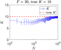
(a)

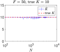
(b)

Figure 1: Estimated number of components $K$ with different $F$ for exponential distribution. The error bars denote one standard deviation away from the mean.

V-B The Swimmer Dataset

We perform experiments on the well-known swimmer [21] dataset, which is widely used for benchmarking NMF algorithms. The swimmer dataset we use contains $256$ binary images ($20$-by-$11$ pixels) which depict figures with four limbs, each can be in four different positions. The latent dimensionality of the corresponding data matrix is $16$. From the regularization path for this dataset presented in Fig. 2, we observe that the estimated latent dimensionality $\hat{K}$ is always $14$ when $10^{-5}\leq\lambda\leq 10^{9}$. In addition, the relative error $\frac{\|\hat{\mathbf{M}}_{2}-\hat{\mathbf{M}}_{2}\hat{\mathbf{X}}\|_{\mathrm{F}}}{\|\hat{\mathbf{M}}_{2}\|_{\mathrm{F}}}$ is close to $0$ when $\lambda\leq 10^{4}$ and becomes intolerably large (larger than $0.75$) when $\lambda\geq 10^{8}$. Therefore, a reasonable estimate for the latent dimensionality is $14$, which is close to the true latent dimensionality.

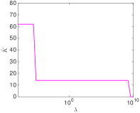
(a)

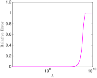
(b)

Figure 2: Estimated number of components and relative error with different $\lambda$ for the swimmer dataset.

VI Future Work

We would like to extend our theoretical analysis to other latent variable models, such as Gaussian mixture models [22, 23] and latent Dirichlet allocation [24, 25]. The parameter $F$ plays an important role in the time complexity of Algorithm 1 and $F$ is very large for certain real data. We may consider combining dimensionality reduction techniques with Algorithm 1 to reduce the running time. Finally, we hope to provide sufficient conditions for the existence of the index set $\mathscr{K}$ such that $\|\mathbf{W}_{2}\mathbf{W}_{1}^{-1}\|_{\infty}<1$ (cf. (64)).

References

• [1] D. D. Lee and H. S. Seung, “Algorithms for non-negative matrix factorization,” in NIPS, 2001, pp. 556–562.
• [2] A. Cichocki, R. Zdunek, A. H. Phan, and S. Amari, Nonnegative matrix and tensor factorizations: applications to exploratory multi-way data analysis and blind source separation, John Wiley & Sons, 2009.
• [3] I. Buciu, “Non-negative matrix factorization, a new tool for feature extraction: Theory and applications,” Int. J. Comput. Commun., vol. 3, no. 3, pp. 67–74, 2008.
• [4] H. Kim and H. Park, “Nonnegative matrix factorization based on alternating nonnegativity constrained least squares and active set method,” SIAM J. Matrix Anal. Appl., vol. 30, no. 2, pp. 713–730, 2008.
• [5] A. Cichocki, R. Zdunek, and S. Amari, “Hierarchical als algorithms for nonnegative matrix and 3D tensor factorization,” in ICA. Springer, 2007, pp. 169–176.
• [6] V. Y. F. Tan and C. Fevotte, “Automatic relevance determination in nonnegative matrix factorization with the $\beta$-divergence,” IEEE Trans. Pattern Anal. Mach. Intell., vol. 35, no. 7, pp. 1592–1605, 2013.
• [7] A. T. Cemgil, “Bayesian inference for nonnegative matrix factorisation models,” Comput. Intell. Neurosci., vol. 2009, 2009.
• [8] O. Winther and K. B. Petersen, “Bayesian independent component analysis: Variational methods and non-negative decompositions,” Digit. Signal Process., vol. 17, no. 5, pp. 858–872, 2007.
• [9] Z. Liu and V. Y. F. Tan, “Rank-one NMF-based initialization for NMF and relative error bounds under a geometric assumption,” IEEE Trans. Signal Process., vol. 65, no. 18, pp. 4717–4731, 2017.
• [10] Y. Li, Y. Liang, and A. Risteski, “Recovery guarantee of non-negative matrix factorization via alternating updates,” in NIPS, 2016, pp. 4987–4995.
• [11] A. Hyvärinen, J. Karhunen, and E. Oja, Independent component analysis, vol. 46, John Wiley & Sons, 2004.
• [12] P. Comon and C. Jutten, Handbook of Blind Source Separation: Independent component analysis and applications, Academic press, 2010.
• [13] A. Anandkumar, R. Ge, D. Hsu, S. M. Kakade, and M. Telgarsky, “Tensor decompositions for learning latent variable models,” J. Mach. Learn. Res., vol. 15, no. 1, pp. 2773–2832, 2014.
• [14] M. E. Davies and Y. C. Eldar, “Rank awareness in joint sparse recovery,” IEEE Trans. Inf. Theory, vol. 58, no. 2, pp. 1135–1146, 2012.
• [15] J. Ziniel and P. Schniter, “Efficient high-dimensional inference in the multiple measurement vector problem,” IEEE Trans. Signal Process., vol. 61, no. 2, pp. 340–354, 2013.
• [16] M. M. Hyder and K. Mahata, “Direction-of-arrival estimation using a mixed $\ell_{2,0}$ norm approximation,” IEEE Trans. Signal Process., vol. 58, no. 9, pp. 4646–4655, 2010.
• [17] G. Obozinski, M. J. Wainwright, and M. I. Jordan, “Support union recovery in high-dimensional multivariate regression,” Ann. Stat., vol. 39, no. 1, pp. 1–47, 2011.
• [18] G. H. Golub and C. F. Van Loan, Matrix computations, vol. 3, JHU Press, 2012.
• [19] D. Malioutov, M. Cetin, and A. S. Willsky, “A sparse signal reconstruction perspective for source localization with sensor arrays,” IEEE Trans. Signal Process., vol. 53, no. 8, pp. 3010–3022, 2005.
• [20] M. Grant and S. Boyd, “CVX: Matlab software for disciplined convex programming, version 2.1,” http://cvxr.com/cvx, Mar. 2014.
• [21] N. Gillis and R. Luce, “Robust near-separable nonnegative matrix factorization using linear optimization,” J. Mach. Learn. Res., vol. 15, no. 1, pp. 1249–1280, 2014.
• [22] D. M. Titterington, A. F. M. Smith, and U. E. Makov, Statistical analysis of finite mixture distributions, Wiley Series in Probability and Statistics, 1985.
• [23] Z. Liu and V. Y. F. Tan, “The informativeness of $k$-means and dimensionality reduction for learning mixture models,” arXiv preprint arXiv:1703.10534, 2017.
• [24] D. M. Blei, A. Y. Ng, and M. I. Jordan, “Latent dirichlet allocation,” J. Mach. Learn. Res., vol. 3, no. Jan, pp. 993–1022, 2003.
• [25] D. Cheng, X. He, and Y. Liu, “Model selection for topic models via spectral decomposition,” in AISTATS, 2015, pp. 183–191.