Climate Modeling of a Potential ExoVenus

Abstract

The planetary mass and radius sensitivity of exoplanet discovery capabilities has reached into the terrestrial regime. The focus of such investigations is to search within the Habitable Zone where a modern Earth-like atmosphere may be a viable comparison. However, the detection bias of the transit and radial velocity methods lies close to the host star where the received flux at the planet may push the atmosphere into a runaway greenhouse state. One such exoplanet discovery, Kepler-1649b, receives a similar flux from its star as modern Venus does from the Sun, and so was categorized as a possible exoVenus. Here we discuss the planetary parameters of Kepler-1649b with relation to Venus to establish its potential as a Venus analog. We utilize the general circulation model ROCKE-3D to simulate the evolution of the surface temperature of Kepler-1649b under various assumptions, including relative atmospheric abundances. We show that in all our simulations the atmospheric model rapidly diverges from temperate surface conditions towards a runaway greenhouse with rapidly escalating surface temperatures. We calculate transmission spectra for the evolved atmosphere and discuss these spectra within the context of the James Webb Space Telescope (JWST) Near-Infrared Spectrograph (NIRSpec) capabilities. We thus demonstrate the detectability of the key atmospheric signatures of possible runaway greenhouse transition states and outline the future prospects of characterizing potential Venus analogs.

1 Introduction

Exoplanetary science lies at the threshold of atmospheric characterization for terrestrial planets. The plethora of exoplanet discoveries from the Kepler mission (Borucki, 2016) revealed that the occurrence rate of planetary sizes increases toward smaller masses (Fressin et al., 2013; Howard, 2013; Petigura et al., 2013) and that there are gaps in the radii distribution that hearken to the effects of planet formation mechanisms (Fulton et al., 2017). The launch of the Transiting Exoplanet Survey Satellite (TESS) will likely find numerous transiting terrestrial planets around bright host stars that are amenable to transmission spectroscopy follow-up observations (Ricker et al., 2015; Sullivan et al., 2015). These planets will produce an unprecedented sample of terrestrial atmospheres from which to study the demographics of comparative planetology (Leconte et al., 2015).

A primary focus of the exoplanet science community is to identify key targets for follow-up observations with ground and space-based survey missions. In particular, the James Webb Space Telescope (JWST) is anticipated to become a major contributor to the measurement and study of exoplanetary atmospheres (Gardner et al., 2006; Bean et al., 2018). With such a large sample of potential targets, it is necessary to apply criteria to decide how valuable follow-up resources will be utilized (Kempton et al., 2018). One such criterion for narrowing the number of follow-up targets is their position relative to the Habitable Zone (HZ), which will allow for atmospheric characterization to focus on planets that may have temperate surface environments (Kasting et al., 1993; Kopparapu et al., 2013, 2014). The methodology of selecting terrestrial planets within the HZ was applied to the Kepler discoveries to construct a catalog of HZ planets for further investigations (Kane et al., 2016). Combining such HZ planet discoveries with statistical techniques with respect to Kepler data sensitivity results in estimates of HZ planet occurrence rates (Kopparapu, 2013; Dressing & Charbonneau, 2015).

However, exoplanet detections using the transit method are intrinsically biased toward short orbital periods (Kane & von Braun, 2008), resulting in a rarity of HZ exoplanet transit detections (except for those planets orbiting very low-mass stars). The vast majority of transit detections lie interior to the HZ where the incident flux on the planet can be many times the solar flux. Thus, many of the exoplanets that will be favorable targets for atmospheric characterization are far more likely to be Venus analogs (exoVenuses) rather than Earth analogs. The frequency of terrestrial planets that may exhibit runaway greenhouse spectral features was quantified with the Venus Zone (VZ) by Kane et al. (2014), with occurrence rates of $0.32^{+0.05}_{-0.07}$ and $0.45^{+0.06}_{-0.09}$ for M dwarfs and GK dwarfs respectively. Several potential Venus analogs were identified, such as Kepler-69b (Kane et al., 2013) and Kepler-1649b (Angelo et al., 2017). The confirmation of a runaway greenhouse hypothesis for these planets, and others like them, depends upon reliable transmission spectroscopy analysis (Kane et al., 2013; Bean et al., 2017).

In order to determine the detectability of particular atmospheric characteristics, we present the results of an exhaustive climate simulation analysis based on the properties of the Kepler-1649 system. In Section 2, we describe the exoplanet Kepler-1649b in detail, highlighting the properties that make it a viable exoVenus candidate. Section 3 details the full range of our climate simulations and the results of that analysis. From our climate models, we generate simulated transmission spectra and identify key spectral features, presented in Section 4. Implications of our study are discussed in Section 5, and we provide concluding remarks in Section 6 including prospects for future observations.

2 A Potential ExoVenus

Considering habitable conditions which would permit the existence of life, Venus-type planets are of particular interest. Although Venus is similar to the Earth in size, density, and composition, the divergence of atmospheric conditions between Venus and Earth has rendered Venus uninhabitable. Thus, studying Venus analogs can elucidate constraints on habitability since such planets can serve as a template for runaway greenhouse conditions that may be the most common scenario of atmospheric evolution for Venus/Earth-size planets, due to the irreversible nature of a runaway greenhouse (Kasting, 1988; Leconte et al., 2013). Furthermore, there are still many features regarding the interior, surface, and atmospheric evolution of Venus that are currently unknown, and a deeper understanding of our sister planet is essential to our interpretation of terrestrial exoplanet data. The present state of Venus knowledge is summarized by Taylor et al. (2018).

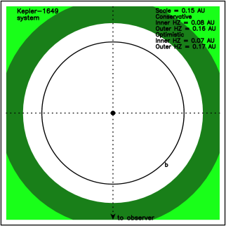
Figure 1: A top-down view of the Kepler-1649 system, showing the host star (intersection of the dotted cross-hairs), orbit of the ‘b’ planet (solid line), conservative HZ (light-green), and optimistic HZ (dark-green). The scale of the figure is 0.15 AU along one edge of the box.

One of the most prominent potential Venus analogs discovered from Kepler observations is Kepler-1649b. The planet has a measured radius of $R_{p}=1.08\pm 0.15$ $R_{\oplus}$ and receives a flux of $F_{p}=2.30\pm 0.65$ $F_{\oplus}$ from its M dwarf host star (Angelo et al., 2017), placing the planet firmly within the VZ of the system. Shown in Figure 1 is a top-down view of the Kepler-1649 system, indicating the relative locations of the planetary orbit (solid line) with respect to the star (intersection of the dotted cross-hairs). The locations of the HZ regions are shown as light-green for the ‘conservative’ HZ and dark-green for the ‘optimistic’ extension to the HZ (Kopparapu et al., 2013; Kane et al., 2016). The inner edge of the optimistic HZ is based on the assumption that Venus could have had surface liquid water as recently as 1 Gya. However, because the surface record has been substantially erased via resurfacing events (Taylor et al., 2018), it is not possible to confirm this hypothesis with currently available in-situ data. Since Kepler-1649b is both similar in size and incident flux to present-day Venus (1.9 versus 2.3 times present-day Earth insolation), it may be considered an archetype of an exoVenus candidate. However, like all VZ and HZ exoplanets, deductions regarding true surface conditions are theories to be tested through climate modeling and further observation.

3 Climate Modeling and Surface Temperature

We attempt to model the atmosphere of Kepler-1649b using an atmosphere with modern Earth constituents quite removed from that of modern Venus. In fact, modeling the climate of Venus is non-trivial due to the dramatic change in atmospheric chemistry that occurs at atmospheric pressures above $\sim$10 bar and the lack of high-temperature line lists for a large range of atomic and molecular species (e.g. Rothman et al., 2013). Numerous climate models have been adapted to the modern Venusian environment in an attempt to model its dynamics and the temperature-pressure variations (Lebonnois et al., 2010; Ando et al., 2016; Lebonnois et al., 2018). Recently, similar such models have been applied to a young, potentially habitable, Venus environment (Way et al., 2016, hereafter Way16). Here we utilize the climate package ‘Resolving Orbital and Climate Keys of Earth and Extraterrestrial Environments with Dynamics’ (ROCKE-3D), described in detail by Way et al. (2017). ROCKE-3D has been used to model a variety of terrestrial planet scenarios, such as synchronous rotation (Fujii et al., 2017) and the effects of variable eccentricity (Way & Georgakarakos, 2017).

A large number of our initial simulations failed because the limit of our radiation tables was rapidly reached. The upper limit is approximately 400 K because we use the HITRAN 2012 database as discussed below. We tested a total of 27 different scenarios in an attempt to reach model stability as close as possible to estimates of Kepler-1649b’s insolation and rotation rate. To that end we slowed the orbital period ($P$), lowered the incident flux ($F_{p}$), decreased the initial CO₂ and CH₄ atmospheric composition, and adjusted the topography and initial surface water. For all scenarios, we assumed that the planet is tidally locked. Tidal locking can have a profound effect on the climate circulation (Kite et al., 2011; Wordsworth, 2015; Koll & Abbot, 2016; Carone et al., 2018; Lewis et al., 2018), and likely occurs on shorter timescales and for longer-period planets than previously determined (Barnes, 2017). Given the relatively short tidal locking timescale for short-period planets, the assumption of tidal locking is sufficiently justified. A list of 10 key selected simulations (from a total of 27), and their final surface conditions is shown in Table 1. These simulations give a summary of our attempts to bring the model to a state as close to Kepler-1649b as possible with ROCKE-3D.

Table 1: Parameters of ROCKE-3D simulations.

ID	$P$	$F_{p}$	Topoa	CO2	CH4	Orbitsb	$T_{\mathrm{mean}}$c	$T_{\mathrm{min}}$	$T_{\mathrm{max}}$	Bald	H2Ostrate	H2Osurff
	(days)	($F_{\oplus}$)		(ppmv)	(ppmv)		(∘C)	(∘C)	(∘C)	(W $\mathrm{m}^{-2}$)	($\mathrm{kg\ kg}^{-1}$)	($\mathrm{kg\ kg}^{-1}$)
1	8.6	2.3	1	400	1	300	90.2	81.2	112.5	103	0.379	0.4845
2	8.6	2.3	3	400	1	66	84.3	42.4	212.4	214	0.099	0.1168
3	8.6	2.3	3	100	0	116	128.9	67.3	285.4	137	0.271	0.3456
4	8.6	2.0	1	400	1	486	91.8	83.5	111.8	77	0.423	0.5214
5	8.6	1.8	1	400	1	634	90.8	83.1	110.2	63	0.434	0.5061
6	8.6	1.6	1	400	1	752	88.0	81.3	102.7	59	0.411	0.4562
7	8.6	1.4	1	400	1	2031	64.1	57.7	72.0	35	0.026	0.1623
8	8.6	1.0	2	400	1	2345	4.3	-54.1	46.9	-3	0.000078	0.0064
9	16.0	1.47	2	400	1	2055	58.3	33.5	91.7	9	0.038	0.1052
10	50.0	1.4	1	376	0	6354	59.0	56.3	61.9	0.3	0.027	0.1226

The ‘Orbits’ column indicates the number of planetary orbits the simulation survived before the climate dynamics became unstable due to the radiation tables moving beyond the valid boundaries of the model. The upper bounds of the ROCKE-3D radiation tables are set by the HITRAN 2012 (Rothman et al., 2013) line list which becomes invalid above 400 K for the gases used in this study. However, in practice, heating rate errors between atmospheric layers will start to grow for temperatures above $\sim$340 K. We use 12 long-wave spectral bands and 24 short-wave bands which allow higher precision than the default SOCRATES Earth specific ga7 spectral files (Edwards, 1996; Edwards & Slingo, 1996). The spectral files were specifically designed for the atmospheres of planets around M dwarfs with higher temperatures and high specific humidities. Typically, once the 400 K limit is reached, the radiation tables start to produce temperature values out of bounds that are indentified by the dynamics code that calculate the heating rates between atmospheric layers (derived from the calculated radiation fluxes). The dynamics code has preset bounds in place that purposely stop the model when these bounds are exceeded.

The mean surface temperatures of the models at the end of the simulations (regardless of whether the bounds were exceeded) are shown in the column labeled ‘$T_{\mathrm{mean}}$’. The topographical model used in each simulation is indicated by the ‘Topo’ column, where the three different categories are defined as follows: aquaplanet (899 m deep all ocean planet), Venus (modern Venus topography, described in Way16), and Venus bath (paleo-Venus topography with all-ocean grid cells set to 1360m in depth). All simulations utilize a Kepler-1649b specific BT-Settl (Allard et al., 2012) spectral distribution file with $T_{\mathrm{eff}}$ = 3200 K, $\log g=5$, and [Fe/H] = 0.

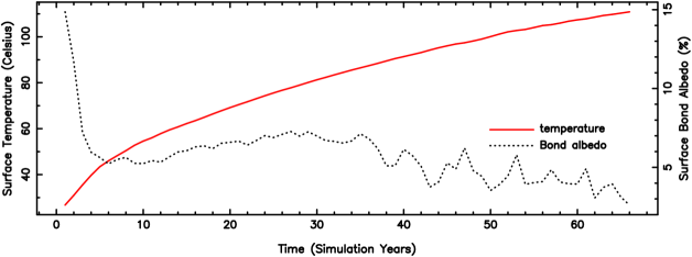
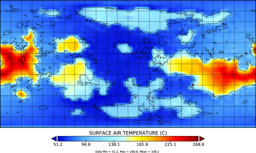
Figure 2: Results from ROCKE-3D Simulation 2 (see Table 1) that utilizes the orbital period and incident flux from Angelo et al. (2017). We adopt a 400/1 CO₂/CH₄ atmosphere and a Venus topography with a liquid water ocean. Top panel: the change in surface temperature (red solid line) and Bond albedo (dotted black line) of the surface as a function of simulation years (orbits). The mean surface temperature at the end of the simulation is 108.2° C. Bottom panel: heat map of the planetary surface at the conclusion of the simulation with the Venus topography overlay. The initial jump in Bond albedo (less so for temperature) is due to the fact that the model starts out with modern Earth initial conditions and it takes time for the model to adjust to the higher insolation being received. See Appendix B “Equilibrium” in Way et al. (2018) for more details regarding how ROCKE-3D comes into net radiative balance, or what we term temperature “equilibrium.”

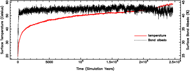
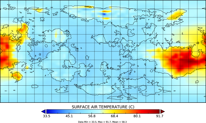
Figure 3: Results from ROCKE-3D Simulation 9 (see Table 1) that utilizes the orbital period and incident flux from Angelo et al. (2017). We adopt a 400/1 CO₂/CH₄ atmosphere and a Venus topography with a liquid water ocean. Top panel: the change in surface temperature (red solid line) and Bond albedo (dotted black line) of the surface as a function of simulation years (orbits). Bottom panel: heat map of the planetary surface at the conclusion of the simulation with the Venus topography overlay. As in Figure 2 the large initial jump in Bond albedo and temperature is due to the fact that the model starts out with modern Earth initial conditions. The mean surface temperature at the end of the simulation is 58.3° C. Note that the length of the simulation and surface air temperature limits are distinct from those in Figure 2.

Our strategy with the simulations in Table 1 was to see whether ROCKE-3D might reach a stable state as we decreased the insolation, adjusted the orbital period, or changed the topography. ROCKE-3D is not capable of accurately modeling the present-day climate of Kepler-1649b, but we demonstrate where the model reaches stable conditions without exceeding the valid ROCKE-3D boundaries (as described above) for a similar system with lower insolation and a longer orbital period. We describe the simulations in detail below.

Simulation 1. Present-day estimates of Kepler-1649b’s insolation and orbital parameters with an aquaplanet topography. The model ran for 300 orbits before errors in the radiative heating fluxes became too great for the radiative transfer scheme and the model crashed.

Simulation 2. The same as Simulation 1, but changed from an aquaplanet to a paleo-Venus-like topography (see Way16) with a $\sim$900m deep bathtub ocean. Different topographies were attempted (not shown herein) because Way16 showed that topography can make a large difference in the climate dynamics and hence surface temperatures. The temperatures in Simulation 2 were similar to those in Simulation 1. The model completed only 66 orbits before crashing for the same reasons as Simulation 1. Figure 2 contains the evolution of the surface temperature and Bond albedo as a function of the orbit number (top panel), and a heat map of the surface temperature with a Venus topography overlay (bottom panel).

The rapid rise in surface temperature (Figure 2, top panel) causes substantial surface H₂O to transfer to the lower atmosphere, and even to the stratosphere. This H₂O transfer process occurs for all of the simulations to varying degrees, as seen in the last two columns of Table 1. As long as surface reservoirs of H₂O exist (lakes and/or oceans) the lower atmosphere will always have more water vapor than the upper atmosphere as it takes time for convection to transport water upward in the atmosphere. The low Bond albedo is probably due to the fact that the only clouds present are at the eastern terminator. It is otherwise a cloud-free sky and this tends to reduce the albedo, as seen in planetary albedo maps produced from the simulation.

Simulation 3. The same as Simulation 2, but with CO₂=100ppmv and CH₄=0 to test how a change in major greenhouse gases would affect the surface temperatures. No improvement was apparent and the model crashed in the radiation after 116 orbits.

Simulations 4–7. The same as Simulation 1, but with insolation lowered from 2.0 times that of present-day Earth to 1.4. As the insolation was lowered, the model completed more orbits while getting closer to equilibrium, yet ultimately still crashed in the radiation.

Simulation 8. The insolation was lowered to present-day Earth (1367 W m^-2) and utilized the same shallow ocean Venus land/sea mask as in Way16. The model completed more orbits and the radiative balance was far closer to our ideal of $\pm$0.2 W m^-2. In this case, the high latitudes began to experience quite low temperatures. ROCKE-3D’s ocean component crashed when a shallow-ocean grid cell at high latitude froze to the bottom. However, unlike the previous simulations, this simulation has the most accurate climate state prediction given its input parameters (columns 2–6 in Table 1) as it is closer to radiative balance than the others.

Simulation 9. To compare with one of the paleo-Venus simulations in Way16 (see Simulation D), we lowered the orbital period to 16 Earth days in length and set the insolation to the same value Venus would have experienced at 2.9 Gya ($F_{p}=1.47$). In the Way16 case, the mean surface temperature reached 56^∘C, while the max was 84^∘C. In Simulation 9 the mean and max were slightly higher at values of 58.3^∘C and 91.7^∘C. Unlike Simulation D in Way16, this simulation crashed as the surface temperatures climbed to values outside the bounds of the ROCKE-3D radiation tables. Figure 3 demonstrates that the surface temperature of Simulation 9 was possibly beginning to stabilize along with the albedo. So this simulation may not be far from equilibrium. Regardless, there are two probable causes for the differences between Simulation D in Way16 and Simulation 9. First, each simulation uses a very different solar spectrum. The Kepler-1649b spectrum is heavily weighted toward the infrared, unlike that of our own sun at 2.9 Gya. There are a number of large water vapor absorption bands in the infrared and these play a role in the increased temperatures (leading to greater heating in the atmosphere and a lower ocean/lake albedo at the surface). Second, while the orbital period of Simulation 9 is 16 Earth days in length, it is not exactly the same as the 16 day long rotation period of Simulation D in Way16. Simulation 9 is tidally locked, and hence the far side of the planet remains in perpetual darkness, whereas Simulation D is not. This will have some influence on the climate dynamics of the model as shown in a suite of ROCKE-3D simulations in Way et al. (2018) Figure 1. The tidally locked world of Simulation 9 will fall more into the regime of the slow rotators of Way et al. (2018) Figure 1 (those with rotation periods of 64 days and longer). There is a transition from circulation that transports heat poleward (rotation periods less 64 days) to a circulation of rising motion on the day side and sinking motion on the night side where transport from day to night occurs over the poles and at the terminator. Yang et al. (2013) has also shown this to be true for tidally locked planets, as is the case for Simulation 9.

Simulation 10. This was a continuation of Simulation 7 with the same insolation, but to see whether the climate dynamics would change substantially if the orbital period was significantly slowed to 50 Earth days in length. Indeed it had a markedly strong effect and this simulation is essentially in equilibrium. Here we see the effect of the single equator-to-pole Hadley cells and the subsequent large cloud bank at the substellar point that increases the planetary albedo and shields the planet from the high insolation of the host star, as first shown in Yang et al. (2014) and explicitly demonstrated for a slowly rotating ancient Venus in Way16.

There are two major caveats to consider when examining the simulations of Table 1. First, the second-to-last column demonstrates the fact that, with the exception of Simulation 8, all of these simulations are well within the moist-greenhouse limit as defined by Kasting (1988); Kasting et al. (1993). Values of the stratospheric water vapor mixing ratio $f$(H₂O) greater than $3\times 10^{−3}$ H₂O to air (kg) push one to this moist-greenhouse limit and most simulations are well above that limit. This implies, according to Kasting et al. (1993) that the timescale for the loss of all of Earth’s ocean water is less than the age of the present-day Earth.

Secondly, we have to consider whether the specific humidity at any atmospheric level is above $\sim$10%. This would indicate that H₂O has become a non-negligible part of the atmospheric mass and errors in the dynamics will begin to increase markedly (see Section 2.1 in Way et al. 2018). Normally the highest values of specific humidity are found at the surface and indeed, with the exception of Simulations 8 and 9, they are all well above 10%.

4 Transmission Spectra and Detectability

The transmission spectrum of Venus has been observed and simulated on numerous occasions. Analysis of transmission spectra from the 2004 transit of Venus by Hedelt et al. (2011) resulted in the detection of CO₂ absorption and was discussed within the context of exoplanets. Similarly, the 2012 transit of Venus afforded an additional opportunity to study a high signal-to-noise transmission spectrum and compare with synthetic spectra of the Venusian atmosphere (García Muñoz & Mills, 2012). Near-infrared observations of Venus have detected water vapor in the Venusian troposphere (Chamberlain et al., 2013). The role of transmission spectra in characterizing exoplanets was discussed by Barstow et al. (2016), emphasizing the effect of clouds in producing ambiguous results. Further simulation of Venusian transmission spectra by Ehrenreich et al. (2012) identified absorption features that originated above the cloud deck that may be used as Venus analog identifiers for exoplanets.

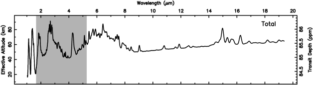
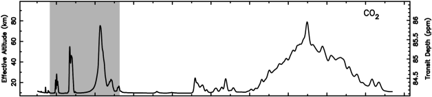
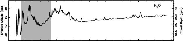
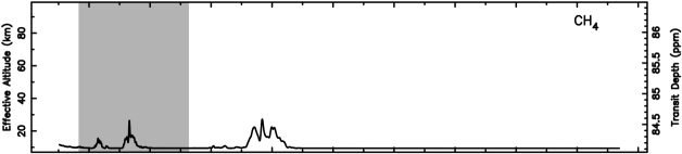
Figure 4: Synthetic 1–20 micron transmission spectra of the Kepler-1649b atmosphere using the results of Simulation 2 (see Section 3 and Table 1). The top panel is the total transmission spectrum including all molecular species. The lower panels, from top to bottom, show the contributions of CO₂, H₂O, CH₄, and N₂ respectively. The shaded region shows the extent of the JWST/NIRSpec passband.

We utilize a publicly available code that was designed to produce transmission spectra from ROCKE-3D output files. The code reads the vertical profiles at the terminator and computes the transmission spectrum, probing each grid cell separately, and accounting for Rayleigh scattering, refraction, and molecular absorption based on HITRAN2012 (Rothman et al., 2013). We applied this code to Simulation 2 (as described in Section 3) since the incident flux for the simulation most closely represents the measurements provided by Angelo et al. (2017) and the Venus topography allows direct comparison with early Venus. The simulated 1–20 $\mu$m transmission spectrum based on the outputs of Simulation 2 is shown in the top panel of Figure 4. The figure also shows the spectrum contributions from the individual components of CO₂, H₂O, CH₄, and N₂. As described in Section 3 and shown in the top panel of Figure 2, the rapid rise in surface temperature results in the transfer of H₂O from the oceans to the atmosphere. This is why the total spectrum shown in Figure 4 is dominated by water vapor. The CO₂ atmospheric content produces substantial absorption features in the 1.5–5.5 $\mu$m range as well as strong absorption effects centered at $\sim$15 $\mu$m. The contributions of both CH₄ and N₂ are negligible apart from small absorption features from CH₄ between 1 and 9 $\mu$m and from a slightly positive N₂ gradient from smaller to longer wavelengths. An important aspect of this transmission spectrum is that it represents the spectrum of a potential transition state of the atmosphere since the climate simulation did not achieve radiative balance. Though the simulation ended before radiative balance was achieved, the clear rise in temperature incidates that the final state of the atmosphere is a runaway greenhouse.

Future prospects are promising for detecting key atmospheric signatures in exoplanets that can help distinguish between Earth and Venus analogs. JWST will revolutionize the field of exoplanet atmospheres by virtue of nearly continuous, long-baseline observations, broader wavelength coverage, and higher spectral resolution than existing ground and space-based facilities (Green et al., 2016). While HST’s Wide-Field Camera 3 (0.8–1.7 $\mu$m) has enabled transit spectroscopy atmospheric characterization for dozens of planets, it is primarily sensitive to water features (Deming et al., 2013), and the interpretation of spectra is highly degenerate and model-dependent (Bean et al., 2018). With broader wavelength coverage and high spectral resolution, JWST will be able to probe a much wider range of chemical species with fewer model assumptions, including the components shown in Figure 4 (CO₂, H₂O, CH₄, and N₂).

JWST is equipped with four visible to mid-IR instruments (NIRCam, NIRISS, NIRSpec, and MIRI) that span 0.6–28 $\mu$m. JWST will have an Early Release Science (ERS) program focused on transiting exoplanets to explore these instruments and exercise their various modes in order to demonstrate their capabilities and characterize their systematics (Bean et al., 2018). The ERS Panchromatic Transmission Program will use NIRISS (0.6–2.8 $\mu$m), NIRCam (2.4–4.0 $\mu$m), and NIRSpec (1.66–5.27 $\mu$m; see Figure 4) to obtain a panchromatic near-IR transmission spectrum of a single planet to calibrate the instruments and establish the best strategies for obtaining transit spectra for future cycles. This program will be particularly important for probing the atmospheres of small exoplanets. This will require knowledge of the noise and systematics and ultimately determine the number of transit observations required to build sufficient precision to detect atmospheric features.

Several studies have investigated the optimal observing strategies for detecting molecular species of small planets orbiting low-mass stars, and have found consistent signal-to-noise requirements of about 10 transits (Morley et al., 2017; Louie et al., 2018; Batalha et al., 2018). These requirements are dependent on both stellar (distance, magnitude, size) and planetary (size, mass) parameters. For the nearby (12 pc) star TRAPPIST-1, which is 18% the mass of the sun, five transit observations are planned with the NIRSpec Prism mode for two of its Earth-sized planets in the HZ (under the JWST Guaranteed Time Observations program). While Kepler-1649b is a prime Venus analog in terms of size and incident flux, the star is comparable in size to TRAPPIST-1 but resides about 67 pc from the sun and is thus relatively faint (Kepler magnitude of 17), which will make it a challenge for follow-up even for JWST. TESS is expected to discover dozens of small planets, including Venus analogs like Kepler-1649b, that orbit nearby bright M-dwarfs (Ricker et al., 2015; Barclay et al., 2018). Many of these planets will be amenable to mass measurements and will be excellent targets for JWST (Kempton et al., 2018) and future Venus analog studies.

5 Discussion

There are numerous proposed causes which can lead atmospheric evolution into a runaway greenhouse state. These include an increase in stellar luminosity (Leconte et al., 2013), an increase in greenhouse gases (Goldblatt et al., 2013), tidal heating for planets in eccentric orbits (Barnes et al., 2013), and a dependence on the latitudinal surface water distribution (Kodama et al., 2018). The simulations presented in this paper primarily focus on the atmospheric evolution after initial conditions that explore a range of atmospheric compositions and surface water initial states. The transition from a surface liquid water state to a full runaway greenhouse is not easily modeled by any 3D climate model, but our simulations do show the transition into a moist greenhouse. It is unclear how long such transitional atmospheric states persist and the synthetic transmission spectra produced for these states, such as the example described in Section 4, may help identify planets which are undergoing such transitions. Note that the transition to a moist greenhouse need not guarantee that a runaway greenhouse will be the final outcome. Indeed it was pointed out by Wordsworth & Pierrehumbert (2013) that a moist greenhouse triggered relatively late in the evolution of the host star such that atmospheric erosion and water loss due to XUV radiation is minimized, could result in a CO₂/H₂O-rich atmosphere that retains surface liquid water.

The follow-up of suitable potential Venus analog targets will require a concerted effort that will utilize the capabilities of such facilities as JWST. There are numerous teams producing simulations using observation times required to fully characterize exoplanet atmospheric signatures, such as the observing strategies proposed by Batalha et al. (2018) and the prioritization framework described by Kempton et al. (2018). As noted earlier, the relative faintness of Kepler-1649 ($J=13.379$) presents a significant challenge in achieving the needed signal-to-noise ratio (S/N) for atmospheric characterization. Equation 1 of Kempton et al. (2018) describes a transmission spectroscopy metric that approximates the S/N for a 10 hr observation with JWST/NIRISS, where Kempton et al. (2018) recommend a S/N $>10$ for terrestrail targets. Using the measured properties of the Kepler-1649 system and the methodology of Kempton et al. (2018), we calculate a transmission spectrum S/N of $\sim$2.1. For a brighter star of $J=10$ ($d=14.1$ pcs), the S/N is $\sim$10.2, and for $J=8$ ($d=5.6$ pcs), the S/N is $\sim$25.6. Therefore, discoveries of similar systems that are much closer to our Sun, such as the discoveries from the TESS mission, will present viable targets to more fully investigate the characteristics of potential runaway greenhouse atmospheres.

6 Conclusions

The celestial sphere has been subjected to intensive monitoring from transit surveys, both from the ground and from space. The photometric precision of these surveys combined with the continuous coverage provided by space-based facilities has changed the shape of the known exoplanet demographics and revealed numerous terrestrial exoplanets. The bias of the transit method toward shorter period planets means that terrestrial planets with incident fluxes substantially higher than that received by the Earth comprise the bulk of the current and near-future discovery space. Hence, in the near term, the majority of the terrestrial exoplanet inventory will reside in a radiation environment that more closely matches that of Venus than of the Earth. This presents a significant challenge since the atmosphere, surface, and interior of Venus have many fundamental questions that have yet to be answered (Taylor et al., 2018). The vast number of terrestrial planet discoveries in the VZ of their host stars makes it imperative that stellar astronomers collaborate with planetary scientists to understand Venusian environments and correctly interpret exoplanet data.

We have presented here a detailed study of the potential Venus analog Kepler-1649b using the ROCKE-3D climate package and adopting a range of starting conditions. Our simulations show that the planetary surface environment is highly likely to exist in a runaway greenhouse state since all of our simulations show a rapid and significant rise in surface temperature when adopting the measured values for the system (Kasting, 1988). These simulations then validate the initial speculation by Angelo et al. (2017) that the planet may indeed be a Venus analog. Our synthetic transmission spectrum for the planetary atmosphere will provide a useful basis for interpreting data acquired for similar planets orbiting brighter host stars that are accessible via future space-based instrumentation. The identification of such Venus analogs will provide invaluable insight into the diversity of exoplanet demographics, evolution of planetary atmospheres, the conditions for runaway greenhouses, and the inner boundaries of habitable planetary surface environments.

References

- Allard et al. (2012) Allard, Y.F., Homeier, D., Freytag, B. 2012, Phil. Trans. R. Soc. A, 370, 2765
- Ando et al. (2016) Ando, H., Sugimoto, N., Takagi, M., et al. NatCo, 7, 10398
- Angelo et al. (2017) Angelo, I., Rowe, J.F., Howell, S.B., et al. 2017, AJ, 153, 162
- Barclay et al. (2018) Barclay, T., Pepper, J., Quintana, E.V. 2018, ApJS, 239, 2
- Barnes et al. (2013) Barnes, R. Mullins, K., Goldblatt, C., et al. 2013, AsBio, 13, 225
- Barnes (2017) Barnes, R. 2017, CeMDA, 129, 509
- Barstow et al. (2016) Barstow, J.K., Aigrain, S., Irwin, P.G.J., Kendrew, S., Fletcher, L.N. 2016, MNRAS, 458, 2657
- Batalha et al. (2018) Batalha, N.E., Lewis, N.K., Line, M.R., Valenti, J., Stevenson, K. 2018, ApJ, 856, L34
- Bean et al. (2017) Bean, J.L., Abbot, D.S., Kempton, E.M.-R. 2017, ApJ, 841, L24
- Bean et al. (2018) Bean, J.L., Stevenson, K.B., Batalha, N.M., et al. 2018, PASP, 130, 114402
- Borucki (2016) Borucki, W.J. 2016, Rep on Prog in Physics, 79, 036901
- Carone et al. (2018) Carone, L., Keppens, R., Decin, L., Henning, Th. 2018, MNRAS, 473, 4672
- Chamberlain et al. (2013) Chamberlain, S., Bailey, J, Crisp, D., Meadows, V. 2013, Icarus, 222, 364
- Deming et al. (2013) Deming, D., Wilkins, A., McCullough, P., et al. 2013, ApJ, 774, 95
- Dressing & Charbonneau (2015) Dressing, C.D., Charbonneau, D. 2015, ApJ, 807, 45
- Edwards (1996) Edwards, J.M. 1996, JAtS, 53, 1921
- Edwards & Slingo (1996) Edwards, J.M., Slingo, A. 1996, QJRMS, 122, 689
- Ehrenreich et al. (2012) Ehrenreich, D., Vidal-Madjar, A., Widemann, T., et al. 2012, A&A, 537, L2
- Fressin et al. (2013) Fressin, F., Torres, G., Charbonneau, D., et al. 2013, ApJ, 766, 81
- Fujii et al. (2017) Fujii, Y., Del Genio, A.D., Amundsen, D.S. 2017, ApJ, 848, 100
- Fulton et al. (2017) Fulton, B.J., Petigura, E.A., howard, A.W., et al. 2017, AJ, 154, 109
- García Muñoz & Mills (2012) García Muñoz, A., Mills, F.P. 2012, A&A, 547, A22
- Gardner et al. (2006) Gardner, J.P., Mather, J.C., Clampin, M., et al. 2006, SSRv, 123, 485
- Goldblatt et al. (2013) Goldblatt, C., Robinson, T.D., Zahnle, K.J., Crisp, D. 2013, Nature Geoscience, 6, 661
- Green et al. (2016) Green, T.P., Line, M.R., Montero, C., et al. 2016, ApJ, 817, 17
- Hedelt et al. (2011) Hedelt, P., Alonso, R., Brown, T., et al. 2011, A&A, 533, A136
- Howard (2013) Howard, A.W. 2013, Science, 340, 572
- Kane & von Braun (2008) Kane, S.R., von Braun, K. 2008, ApJ, 689, 492
- Kane et al. (2013) Kane, S.R., Barclay, T., Gelino, D.M. 2013, ApJ, 770, L20
- Kane et al. (2014) Kane, S.R., Kopparapu, R.K., Domagal-Goldman, S.D. 2014, ApJ, 794, L5
- Kane et al. (2016) Kane, S.R., Hill, M.L., Kasting, J.F., et al. 2016, ApJ, 830, 1
- Kasting (1988) Kasting, J.F. 1988, Icarus, 74, 472
- Kasting et al. (1993) Kasting, J.F., Whitmire, D.P., Reynolds, R.T. 1993, Icarus, 101, 108
- Kempton et al. (2018) Kempton, E.M.-R., Bean, J.L., Louie, D.R., et al. 2018, PASP, 130, 114401
- Kite et al. (2011) Kite, E.S., Gaidos, E., Manga, M. 2011, ApJ, 743, 41
- Kodama et al. (2018) Kodama, T., Nitta, A., Genda, H., et al. 2018, JGRE, 123, 559
- Koll & Abbot (2016) Koll, D.D.B., Abbot, D.S. 2016, ApJ, 825, 99
- Kopparapu (2013) Kopparapu, R.K. 2013, ApJ, 767, L8
- Kopparapu et al. (2013) Kopparapu, R.K., Ramirez, R., Kasting, J.F., et al. 2013, ApJ, 765, 131
- Kopparapu et al. (2014) Kopparapu, R.K., Ramirez, R.M., SchottelKotte, J., et al. 2014, ApJ, 787, L29
- Lebonnois et al. (2010) Lebonnois, S., Hourdin, F., Eymet, V. et al. 2010, JGRE, 115, E06006
- Lebonnois et al. (2018) Lebonnois, S., Schubert, G., Forget, F., Spiga, A. Icarus, 314, 149
- Leconte et al. (2013) Leconte, J., Forget, F., Charnay, B., Wordsworth, R., Pottier, A. 2013, Nature, 504, 268
- Leconte et al. (2015) Leconte, J., Forget, F., Lammer, H. 2015, ExA, 40, 449
- Lewis et al. (2018) Lewis, N.T., Lambert, F.H., Boutle, I.A., et al. 2018, ApJ, 854, 171
- Louie et al. (2018) Louie, D.R., Deming, D., Albert, L., et al. 2018, PASP, 130, 044401
- Morley et al. (2017) Morley, C.V., Kreidberg, L., Rustamkulov, Z., Robinson, T., Fortney, J.J. 2017, ApJ, 850, 121
- Petigura et al. (2013) Petigura, E.A., Marcy, G.W., Howard, A.W. 2013, ApJ, 770, 69
- Ricker et al. (2015) Ricker, G.R., Winn, J.N., Vanderspek, R., et al. 2015, JATIS, 1, 014003
- Rothman et al. (2013) Rothman, L.S., Gordon, I.E., Babikov, Y., et al. 2013, JQSRT, 130, 4
- Sullivan et al. (2015) Sullivan, P.W., Winn, J.N., Berta-Thompson, Z.K., et al. 2015, ApJ, 809, 77
- Taylor et al. (2018) Taylor, F.W., Svedhem, H., Head, J.W. 2018, SSRv, 214, 35
- Way et al. (2016) Way, M.J., Del Genio, A.D., Kiang, N.Y., et al. 2016, GeoRL, 43, 8376
- Way & Georgakarakos (2017) Way, M.J., Georgakarakos, N. 2017, ApJ, 835, L1
- Way et al. (2017) Way, M.J., Aleinov, I., Amundsen, D.S., et al. 2017, ApJS, 231, 12
- Way et al. (2018) Way, M.J., Del Genio, T., Aleinov, I., Clune, T., Kelley, M., Kiang, N. 2018, ApJS, in press (arXiv:1808.06480)
- Wordsworth & Pierrehumbert (2013) Wordsworth, R.D., Pierrehumbert, R.T. 2013, ApJ, 778, 154
- Wordsworth (2015) Wordsworth, R.D. 2015, ApJ, 806, 180
- Yang et al. (2013) Yang, J., Cowan, N.B., Abbot, D.S. 2013, ApJL, 771, L45
- Yang et al. (2014) Yang, J., Boué, G., Fabrycky, D.C., Abbot, D.S. 2014, ApJL, 787, L2
- Young (1980) Young, L.G. 1980, Icarus, 43, 102
- Young (1982) Young, L.G. 1982, Icarus, 51, 606