Back to “Normal” for the Disintegrating Planet Candidate KIC 12557548 b

Abstract

KIC 12557548 b is first of a growing class of intriguing disintegrating planet candidates, which lose mass in the form of dust particles . Here, we follow up two perplexing observations of the system: 1) the transits appeared shallower than average in 2013 and 2014 and 2) the parameters derived from a high resolution spectrum of the star differed from other results using photometry and low resolution spectroscopy. We observe 5 transits of the system with the 61-inch Kuiper telescope in 2016 and show that they are consistent with photometry from the Kepler spacecraft in 2009-2013. We also evaluate high resolution archival spectra from the Subaru HDS spectrograph and find them to be consistent with a main-sequence T_eff=4440 $\pm$70 K star in agreement with the photometry and low resolution spectroscopy. This disfavors the hypothesis that planet disintegration affected the analysis of prior high resolution spectra of this star. We apply Principal Component Analysis to the Kepler long cadence data to understand the modes of disintegration. There is a tentative 491 day periodicity of the second principal component, which corresponds to possible long-term evolution of the dust grain sizes, though the mechanism on such long timescales remains unclear.

1 Introduction

Rappaport et al. (2012) first reported the discovery of a highly unusual system in the Kepler field, KIC 12557548. Its light curve exhibits flux dips with a period of 0.654 days. Surprisingly, the flux dips are neither symmetric in shape nor constant in amplitude, varying from $\sim$0% to $\sim$1.2%. The amplitudes of the flux dips are highly stochastic and unpredictable from one event to the next 0.654 days later. This is radically different from a transiting planet, where the planet absorbs the same amount of light from the star each orbit and does so symmetrically about the star, modulo stellar inhomogenities. The time variability of the flux dips indicates that material with a projected area $\sim$1% of the stellar surface is created and cleared in $\lesssim$ 1 day timescales in order to extinct $\sim$1% of starlight at one epoch and $\sim$0% at another. These unusual light curve behaviors are best explained as dust extinction from a comet-like tail of material that is escaping a rocky planet (KIC 12557548 b, hereafter KIC 1255 b) in a short period orbit. The comet-like shape of the dust explains the asymmetric shape of the light curve profile. The KIC 12557548/KOI-3794/Kepler-1520 system (hereafter KIC 1255) has the exciting possibility of being an opportunity to study a planet that has been peeled away layer by layer to reveal an interior core.

After the discovery of KIC 1255, other systems were found to show similar light curve behavior: K2-22 (Sanchis-Ojeda et al., 2015), WD 1145+017 (Vanderburg et al., 2015) and KOI 2700 (Rappaport et al., 2014) . A collection, albeit small, of several different disintegrating planet systems makes for a useful laboratory for understanding planet evolution and composition. Multi-wavelength light curve measurements show that the dust particles inferred to be escaping from these objects can have wavelength-dependent transmission, as predicted for sub-micron dust particles (Bochinski et al., 2015; Sanchis-Ojeda et al., 2015).

Furthermore, there are perplexing systems that also display stochastic transit behavior but for which there are still no fully agreed-upon explanations: KIC 8462852 (ie. Boyajian’s star) (Boyajian et al., 2016), RIK-210/EPIC 205483258 (David et al., 2017) and PTFO 8-8695 (van Eyken et al., 2012). KIC 8462852 may be a family of comets from one or more parent bodies that recently broke apart (Boyajian et al., 2016; Bodman & Quillen, 2016; Wright & Sigurdsson, 2016). RIK-210 and PTFO 8-8695 are both in young systems ($\lesssim$ 10 and $\lesssim$3 Myr, respectively), so they may be proto-planet candidates or structures within a protoplanetary disk (Stauffer et al., 2017; Yu et al., 2015). RIK-210 could be accreting material that causes variable extinction while PTFO 8-8695’s orbit may be precessing and causing variations in transit depth depending on its longitude, though only portions of the lightcurve are explained this way (Barnes et al., 2013; Yu et al., 2015).

The Kepler spacecraft performed near-continuous long cadence photometry of KIC 12557548 during its entire main mission lifetime from 2009 to 2013. During this time, the transit depths averaged around $\sim$0.6% but varied stochastically from just one 15.7 hour orbit to the next. van Werkhoven et al. (2014) analyzed 15 of the total 17 quarters of data and calculated every transit depth during this period. There were two intervals near obits 50 and 1950 that showed shallower (0.1%) than average transit depths for roughly one month in duration.

The underlying planet candidate KIC 1255 b has not been detected directly, but several observational constraints have placed upper limits on its size and mass. High precision radial velocity measurements of the host star with Keck/HIRES put an upper limit on the reflex motion due to the planet and constrains the mass to be $\lesssim 1.2M_{\mathrm{J}up}$ (Croll et al., 2014). Masuda et al. (2018) find that the upper limit on the radial velocity semi-amplitude is 86 m/s corresponding to a planet mass $\lesssim 0.28M_{\mathrm{J}up}$ using the Subaru High Dispersion Spectrometer (HDS). There is no detection of secondary eclipses of KIC 1255 b with a 3$\sigma$ upper limit of $5\times 10^{-5}$ in the Kepler bandpass, which means that for an albedo of 0.5, the radius of the planet must be smaller than 4600 km (van Werkhoven et al., 2014). A radiative-hydrodynamic wind model predicts that the mass loss rate will be a strong function of planet mass and for the present-day mass loss rate of $\sim$ M${}_{\oplus}/Gyr$ (determined by the mass of dust needed to absorb and scatter 10^-2 of star light per orbit), the modeled mass is 0.014 $M_{\oplus}$ (Perez-Becker & Chiang, 2013).

One possible explanation for the planet disintegration is that it is tied to stellar activity. Kawahara et al. (2013) found an anti-correlation between stellar flux and the depth of transit events and suggested that the alignment of the planet’s position (true anomaly) with active regions on the star causes disintegration. The alignment of spots and disintegration activity could be due to XUV photoevaporation or magnetic reconnection events. The anti-correlation between stellar flux and transit depth was confirmed by Croll et al. (2015), though the authors find that occultations of star spots can also modulate the transit depth at the 22.9 day rotation period of the star.

The Kepler data was used to put constraints on the particle size distribution and composition of the dust particles. Budaj (2013) and Brogi et al. (2012) modeled the light curve, which includes a slight increase in flux before the transit begins. This pre-ingress flux increase is caused by forward scattering dust particles and the scattering function is sensitive to particle size modulo composition. Budaj (2013) and Brogi et al. (2012) find particle sizes $\sim$0.1 to $\sim$1.0$\mu$m in size based on this method. The tail length can also be used to constrain the composition of the particles and van Lieshout et al. (2014) find that the sublimation times of corundum and iron-rich silicates are consistent with the observed tail lengths.

Multiple wavelength monitoring can also constrain the dust particle sizes because the scattering by dust is a strong function of wavelength. Bochinski et al. (2015) observed wavelength dependence in the transits by KIC 1255 b and find that the extinction is similar to the ISM particles with sizes from 0.25 to 1 $\mu$m. Subsequently, Croll et al. (2014) obtained a $K^{\prime}$-band light curve simultaneously with the Kepler spacecraft to put a constraint on the dust extinction as a function of wavelength. Croll et al. (2014) find a particle size distribution of $\gtrsim 0.5\mu$m. Recent modeling by Ridden-Harper et al. (2018) shows that the wavelength-dependent extinction function could be due to the tail’s changing optical thickness.

Schlawin et al. (2016) observed 8 total transits of the system for 4 nights in 2013 and 4 nights in 2014 for the $r^{\prime}$ band using the MORIS imager (Gulbis et al., 2011) on SpeX/IRTF (Rayner et al., 2003). The SpeX/IRTF spectrum, though affected by systematic noise, confirmed the Croll et al. (2014) result that particle sizes are $\gtrsim 0.5$ $\mu$m for a pyroxene composition. Schlawin et al. (2016) found that the optical transit depths were all weaker than $0.43\%$ and that the probability of this randomly occurring based on random behavior from Kepler statistics was around 0.2%. This was evidence that the observations occurred during weaker periods (as found in van Werkhoven et al. (2014)’s 15 Kepler quarter analysis) or that the disintegration activity was falling off with time. We performed follow-up $R$ band photometry of the KIC 1255 system to explore these two hypotheses and see if the the disintegration has returned to the levels found in the Kepler mission and discuss this in Section 2. We also re-analyzed the Kepler photometry in order to quantify the light curve behavior in comparison to ground-based photometry in Section 3.

The high resolution spectrum of KIC 1255 (Kawahara et al., 2013) showed a different temperature and gravity than photometric methods (e.g. Brown et al., 2011; Huber et al., 2014). van Lieshout et al. (2016) suggest that one exciting possibility is that gases from the disintegrating planet contaminate the high resolution spectrum. This would enable compositional and kinematic studies of the disintegrating planet. In Section 4, we examine archival Subaru High Dispersion Spectrograph (HDS) spectra of the star to assess the stellar parameters and explore the possibility that sublimated gases appear in the high resolution spectrum. We conclude in Section 5.

Table 1: List of photometric observations

Date	Weather	Airmass	Seeing	Amplitude, $A$
UT			(″)
2016 Jun 10	Cloudy	$\cdots$	$\cdots$	$\cdots$
2016 Jun 12	Clear	1.29 $\rightarrow$ 1.06 $\rightarrow$ 1.10	1.3	0.94 $\pm$ 0.16
2016 Jun 14	Clear	1.47 $\rightarrow$ 1.06 $\rightarrow$ 1.12	1.4	0.70 $\pm$ 0.18
2016 Jul 12	Clear	1.19 $\rightarrow$ 1.06 $\rightarrow$ 1.63	1.2	0.78 $\pm$ 0.14
2016 Jul 14	Mostly clear	1.24 $\rightarrow$ 1.06 $\rightarrow$ 1.55	1.2	1.33 $\pm$ 0.14
2016 Jul 16	Clear	1.36 $\rightarrow$ 1.06 $\rightarrow$ 1.26	1.4	2.14 $\pm$ 0.19

2 Photometric Observations

We attempted to observe 6 transit events of KIC 1255 b with the Mont4k imager on the 61-inch Kuiper telescope located on Mt Bigelow, Arizona in 2016 using the f/13.5 Cassegrain focus. On all nights we used 90 second exposures using a Harris-R filter to best approximate the $r^{\prime}$ filter used in Schlawin et al. (2016). 5 of the 6 nights were clear with the exception of a few passing clouds on UT 2016 Jul 14. Cloudy skies on UT 2016 Jun 10 prevented high precision time series. Table 1 shows a summary of our observations and the UT dates. The data was taken in a 3x3 binning mode resulting in an effective 0.43”/pixel plate scale.

2.1 Photometric Pipeline

For the photometric reduction, we used the Python ccdproc package (Craig et al., 2015) to generate master flat field and bias files. They were combined with an average with a low threshold of 2$\sigma$ and a high threshold of 5$\sigma$.

We used the Python photutils v0.3 (Bradley et al., 2016) package to centroid and extract fluxes of the KIC 1255 and the reference stars. We used a photometric aperture of 9 pixels (3.9”) and a background annulus from 9 to 12 pixels (3.9” to 5.2”) on all stars and nights. 12 stable reference stars with similar R band brightnesses were used to construct a reference time series to correct for variable telluric and instrument throughput. The reference stars are identified Figure 1 across the 9.7′$\times$ 9.7 ′ Mont4K field of view. These 12 reference stars’ time series were combined with a weighted average and this combined time series was divided into the target, KIC 1255.

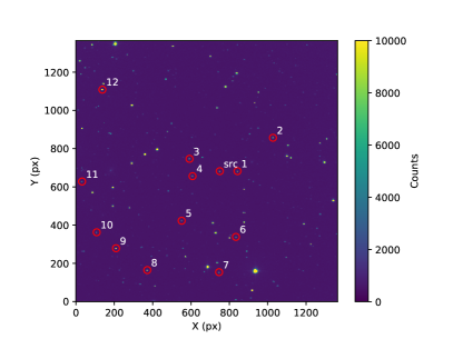
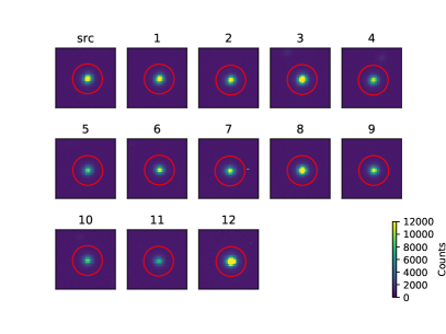
Figure 1: Left: KIC 1255 (src) and reference stars (numbered) used on UT 2016-07-14 are shown over the full 9.8′$\times$ 9.8′ Field of View of Mont4K . Right: Postage stamp zoom-ins for the source and reference stars show the point spread functions for each star. The reference stars were chosen to have similar count levels as KIC 1255.

All light curves for KIC 1255 and the 12 reference stars are shown in Figure 2. These are the same reference stars shown in Figure 1. The two nights 2016 Jun 12 and 2016 Jun 14 show greater overall stability than the 3 nights in July, 2016. We suspect that the higher moisture levels and occasional cloud passages (such as the ones that caused huge drops in flux on UT 2016 Jul 14) affected the later observations.

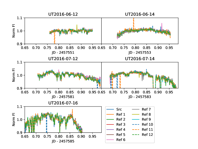
Figure 2: Time series photometry for all stars and all nights. The nights in July appear more strongly affected by cloud/and or seeing variations, whereas the two nights in June are stable to within a few percent. All source radius, background start and background annulus end parameters were 9, 9 and 12 pixels respectively.

2.2 Transit Depth Fitting

Figure 3 shows the reference-corrected time series for KIC 1255 for all nights. We use the planet transit ephemeris from Croll et al. (2015) where the Kepler flux minimum is the “transit center”:

$$T=T_{0}+nP$$ (1)

where $T_{0}=2454968.9820\pm 0.0007$ BJD_TDB and $P=0.6535534\pm 0.0000002$ days. The expected transit epochs from this ephemeris are shown for reference as vertical red bars. Typical uncertainties for the Kepler ephemeris are $\sim$ 1 minute at these dates due to the large number of transits measured by the Kepler observatory over nearly 4 years. The “transit duration” from Kepler light curves is about 0.06 days, which is consistent with these transit durations.

We find the best fit to each light curve using the average Kepler short cadence light curve as a model. We include a linear baseline so that the model is

$$F(t)=\left(A\cdot f_{SC}(t)+1\right)(1+B+C\cdot t),$$ (2)

where $F(t)$ is the normalized flux at orbital phase $t$, $A$ is the amplitude parameter, $f_{SC}(t)$ is average Kepler short cadence light curve linearly interpolated at an orbital phase $t$, $B$ is the baseline offset and $C$ is the baseline slope. We construct $f_{SC}(t)$ by phasing the Kepler time series with Equation 1, dividing by a quadratic baseline from each transit, averaging the results and subtracting 1.0 to get the differential flux. We use the Markov Chain Monte Carlo (MCMC) package emcee (Foreman-Mackey et al., 2013) to find the transit depth amplitude and uncertainty. We use 50 MCMC chains with 500 burn-in points and 1500 points to sample the posterior distribution. The best-fit light curves are shown in Figure 3 and the best-fit amplitudes are listed in Table 1.

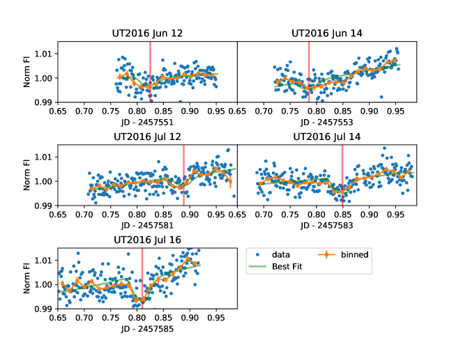
Figure 3: Reference-corrected time series photometry of KIC 1255 for all nights (blue circles). Orange squares mark 20 minute flux bins for visual clarity. The expected transit epochs from the Kepler-based ephemeris (Croll et al., 2015) are shown as vertical red bars. We also fit each light curve with a model that scales the average Kepler short cadence data (Equation 2) shown in green. Transits are clearly visible for all nights except for UT 2016 Jun 14.

To ease the visual comparison of the models and measured data, we bin the 61-inch Mont4K data into 20 minute long bins, shown in Figure 3. Obvious cosmic ray outliers were discarded by removing points (at any epoch within the reference-corrected time series) with fluxes below 0.98 and above 1.02 times the median flux for the night. The error bars for the binned data are calculated from the standard error in the mean for each bin. When calculating the best fit model and posterior distribution of parameter, however, the un-binned data is used.

In contrast to Schlawin et al. (2016), the transit depths in 2016 June and 2016 July are similar to the distribution measured by the Kepler spacecraft from 2009 to 2013. Schlawin et al. (2016) found significantly weaker transit depths that the Kepler spacecraft in 2013 Aug-Sep and 2014 Aug-Sep, which indicated that either disintegration activity was slowing down or that there were quiescent periods during those observations. The transit depths listed in Table 1 are “back to normal” in that they are consistent with the Kepler results. We will revisit the statistics of these events in Section 3.4.

3 Kepler Re-analysis

We examine the 17 total quarters of Kepler data to understand the statistics of the transits and put the 2013-2016 observations in context. Mainly, we sought to evaluate the likelihood of the weak transits observed in 2013-2014 and normal transits in 2016. We downloaded all 17 quarters of Kepler Long-Cadence data from the MAST archive beginning on 2009 May 13 and ending on 2013 April 08 for a total of 1425 days or 2181.5 orbits. The Kepler data were examined for one transit or secondary eclipse at a time with a window of $\pm$0.28 in orbital phase. A quadratic baseline is fit to all the points before a phase of -0.12 and after a phase of 0.15 within the $\pm$ 0.28 phase window. The -0.12 and 0.28 phases are set from the points within the average Kepler light curve that are within $\pm$ 200 ppm from the median out-of-transit flux. All points are divided by this baseline to produce a normalized flux transit or eclipse profile. The secondary eclipses are used to quantify the noise in the transit depths.

3.1 Kepler Secondary Eclipse

We confirm the result of van Werkhoven et al. (2014) that no secondary eclipse is detected at f_p/f_∗ $\lesssim 50$ ppm, where f_p/f_∗ is the relative flux of the planet to star in the Kepler bandpass, as seen in Figure 4. We then use the secondary eclipses as a way to characterize the noise of the primary transits. Both have the same quadratic baseline removal process over the same time intervals.

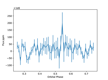
Figure 4: No secondary eclipse (f_p/f_∗ $\lesssim$ 50 ppm) is detected from a phase range of 0.25 to 0.75, even with 17 quarters (4 years) of Kepler Long Cadence data. Here, the data are binned to orbital phases of 0.016 (15 minutes) and errors calculated from the standard error in the mean of the data within a bin.

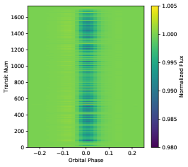
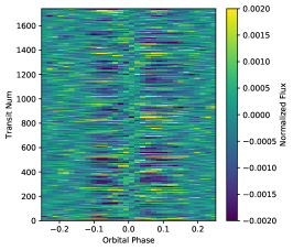
Figure 5: Cleaned Kepler Long-cadence data (Left) and model fit using the average light curve (Middle). The residuals (Right) show significant deviations near phases of -0.05 and 0.05.

3.2 Average Light Curve Analysis

In order to perform some analysis techniques on the data and to study the transit depth behavior, we first create a uniform cleaned two dimensional array of the time series. We linearly interpolated the Kepler long-cadence data set onto a fixed phase grid with a spacing of 15 minutes (to Nyquist sample the 30 minute observation cadence) and put together all the time series that have no gaps into this two dimensional grid. This cleaned Kepler long-cadence array is shown in Figure 5.

We start by taking the average transit light curve of all the long cadence data (the mean of the 2D grid along the transit number axis). We then take the dot product ($\bullet$) with this average light curve to create an amplitude time series.

$$A^{\prime}\equiv\frac{(f-1)\bullet\vec{a}}{\vec{a}\bullet\vec{a}},$$ (3)

where $\vec{a}$ is the amplitude vector, $f$ is the flux matrix with x indices of time and y indices of transit number and $a$ is the average spectrum. This dot product, $A^{\prime}$ is comparable to the transit amplitude $A$ in Equation 2.

This dot product is then multiplied by the average transit light curve to create a 2D model grid. The residual of this model (Figure 5) shows significant $\pm$0.2% deviations from white noise, indicating that the dusty tail surrounding KIC 1255 b changes in shape (or scattering properties) with time. We explore more sophisticated models than the average light curve below that are based on principal component analysis. However, this average model serves as a useful comparison to fitting the transit depth for ground-based photometry, as performed in Section 2.2. The 0.2% residuals with this average model are comparable with the typical photometric scatter of $\sim$ 0.1% to 0.2% for 20 minute timescales in Schlawin et al. (2016) and this work. We statistically compare the transit depths from the Kepler mission from 2009 to 2013 to the ground-based measurements from 2013 through 2016 in Section 3.4.

3.3 Principal Component Analysis

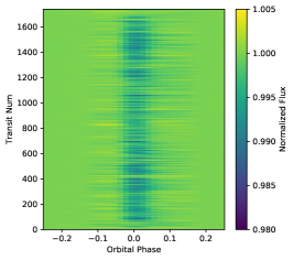
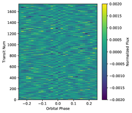
Figure 6: Cleaned Kepler Long-cadence data (Left) and model fit using 4 Principal Components (Middle). The residuals are $\lesssim 0.1\%$ (Right), significantly smaller than the $\sim 0.2\%$ residuals when using the average-light curve method shown in Figure 5.

As another way of analyzing the light curve data, we apply Principal Component Analysis (PCA) to this two dimensional grid. Here, we are assuming that the grid of orbital phases (spaced by 15 minutes) contains random correlated variables with different realizations along the transit number axis. The first principal component eigenvector is the linear combination of these random variables that maximizes the variance in the flux. The second principal component eigenvector is the linear combination of these random variables with the next-highest variance while being orthogonal to the first principal component. This continues up to some finite number of principal components, with the hope that we can use a few orthogonal light curves to adequately describe the data (e.g. Jolliffe, 2002). We use the Python package scikit-learn (Pedregosa et al., 2011) to calculate the principal components and eigenvectors.

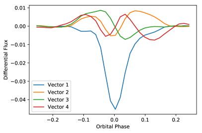
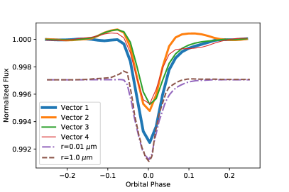
Figure 7: The principal component eigenvectors scaled by their eigenvalues (Left), shows that the first eigenvector largely describes the extinction while the second shows the contributions from forward scattering. When the eigenvectors are transformed into light curves (Right), it can be seen that the first eigenvector corresponds to small dust particle sizes with negligible forward scattering (dash-dot purple model Budaj, 2013). The second eigenvector resembles models with large dust particle sizes with pronounced forward scattering before and after the transit mid-point (dashed brown model Budaj, 2013). The models are offset vertically for clarity.

We use a covariance matrix as opposed to correlation matrix to calculate the principal component eigenvectors. In other uses of PCA, the variables are often scaled so that they all have a variance of 1.0 to ensure that variables with intrinsically larger variance (such as height in inches over weight in kilograms) do not get higher loadings in the principal component eigenvectors (Jolliffe, 2002). However, we do not scale the variables (columns) by variance and use a covariance matrix because all of our variables are the same units (normalized flux). If we scaled each column in this 2D grid by its standard deviation or used a correlation matrix, this would magnify the contribution of photon noise to out-of-transit data over the real astrophysical variability of the inner phases (between $\sim$ -0.12 to $\sim$0.15).

The model using the first 4 principal components shown in Figure 6 better matches the data and has residuals much closer to white noise than the model that uses the dot product with the average light curve.

Figure 7 shows the first 4 eigenvectors as a function of orbital phase. For the eigenvectors plot, we multiply each eigenvector by its eigenvalue to emphasize the relative covariances between the principal components and phase grid variables. The first 4 eigenvectors explain 62%, 12%, 6% and 3% of the variance (a total of 84%) for the 32 points (variables) in the phase grid from -0.25 to 0.25. We also transform the eigenvectors into light curves by multiplying each eigenvector by the standard deviation of principal components and adding it to the average light curve, as shown in the right side of Figure 7.

The first eigenvector largely corresponds to models of small dust grains with more isotropic scattering so that the light curve is dominated by extinction (Budaj, 2013; Brogi et al., 2012). We also note that the second eigenvector resembles models of large dust grains of pyroxene from Budaj (2013), where the particles that are a similar order of magnitude as the wavelength exhibit forward scattering, which causes a pronounced pre-ingress flux increase. The second eigenvector has a broader forward scattering peak than the Budaj (2013) models, so it may be the result of a broader distribution of particles. The fact that the pre-ingress flux increase is not found in the first eigenvector and instead is pronounced in orthogonal eigenvectors suggests that the dust particle sizes may be changing in time. We would expect that a dust tail with a variable number of particles but a constant grain size would exhibit a forward scattering in the first principal component because the forward scattering flux would scale proportionally with the number of particles and transit depth. The implication of the PCA then is that the dust particle sizes may be changing with time.

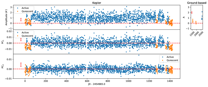
Figure 8: Time series of the transit amplitude and principals components of the Kepler data (Left panel). We also show the ground-based photometry from Schlawin et al. (2016) and this work (Right upper plot). Quiescent intervals with low transit activity are identified from the amplitude The first principal component tracks closely with the amplitude. The second principal component shows periodicity at 491 days, indicating possible long-term evolution of dust grain particle sizes.

Figure 8 shows the time series of the first two principal components (PC₁ and PC₂). We highlight the quiescent periods, which are also discussed in Kawahara et al. (2013), van Werkhoven et al. (2014) and Croll et al. (2015). The first principal component largely tracks closely with the dot product of the average light curve ($A^{\prime}$). The quiescent periods show up as 14 to 36 day long intervals of low amplitude events. The second principal component shows some sinusoidal behavior at a $\sim$500 day period, indicating that the large particles may be evolving. However, the timescale of these sinusoidal modulations of PC₂ is much longer than dynamical time (t${}_{dyn}\sim$ P = 0.65 days) and sublimation times ($t_{sub}\sim$1 day Rappaport et al., 2012) for this system.

In Figure 9 we show the periodogram of the principal components. The first component, corresponding to the transit depth, has peaks at 22.9, 153 and 750 days. The 22.9 day peak is consistent with the Kawahara et al. (2013) and Croll et al. (2015) that shows amplitudes are anti-correlated with stellar flux. As suggested in Kawahara et al. (2013), the anti-correlation points to a physical mechanism for the disintegration - such as magnetic activity or high energy flux associated with spots causing disintegration on the planet. The second principal component’s periodogram has a strong peak at 491 days. This singly-peaked periodogram implies that PC₂ is nearly sinusoidal. As shown in Figure 7, the second principal component resembles models with larger dust grains, so the dust grain sizes could be evolving on long-term 491-day timescales. This is much longer than the dynamical and sublimation times of the system, so there is no obvious mechanism for the dust grain size evolution. It is also possible that red noise such as 1/$f$ noise contributes to these long term oscillations.

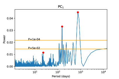
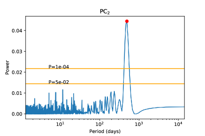
Figure 9: Periodograms of the principal component time series shown in Figure 8, with peaks marked with red circles. PC₁ peaks at 22.9, 153 and 750 days. The 22.9 day peak is consistent with Kawahara et al. (2013), who notice that this period is co-incident with the stellar rotation period. The second principal components shows one dominant peak at 491 days, indicating possible long term evolution of the dust particle sizes.

3.4 Statistical Analysis of Ground-based Photometry

We calculate and evaluate the Kepler transit amplitudes to compare to ground-based results and to understand the long-term behavior of KIC 1255 b’s disintegration. We take the histogram of transit amplitudes as measured by the Kepler light curves (shown in Figure 10) and compare these to the ground-based photometry from Schlawin et al. (2016) and this work. The histogram of secondary eclipse amplitudes from the Kepler light curves is also plotted in Figure 10, which shows the spread due to photon noise. The intrinsic astrophysical variation of the planet disintegration is convolved by this photometric scatter in the data.

We compare the distribution of amplitudes from Schlawin et al. (2016) from the Kepler long cadence data from 2009 to 2013. A Kolmogorov-Smirnov (KS) test gives a $p$ value of 0.001 of the null hypothesis that the Schlawin et al. (2016) results are drawn from the same distribution as the Kepler Long Cadence data. This indicated a possible slowdown of disintegration activity. However, the distribution from this work taken in 2016 shows consistency with the Kepler histogram, with the KS test $p$ value of 0.5 of the null hypothesis. We therefore conclude that the disintegration activity is stochastic with no long-term slowdown measurable from ground-based photometry.

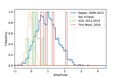
Figure 10: Normalized frequency of 4 different amplitude distributions: 1) all of the Kepler Long Cadence data during transit from 2009 to 2013, 2) the secondary eclipse amplitudes from the Kepler spacecraft over this same period, 3) the 8 night ground-based IRTF transit campaign in the summers of 2013 and 2014 from Schlawin et al. (2016) (S16) and 4) the 5 night Kuiper telescope transit campaign in the summer of 2016. The Schlawin et al. (2016) (S16) events give a KS-test $p$ value of 0.001 when comparing to the Kepler data. In contrast, the 2016 photometric results in this work are consistent with the Kepler Long Cadence data, giving a $p$ value of 0.5. This indicates that the transit depths are back to normal and there is no slowdown of disintegration activity over time.

4 Stellar Characterization

4.1 Previous Observations

Table 2: Observational estimates of the stellar parameters of KIC 1255, adapted from van Lieshout et al. (2016)

Reference	$T_{\mathrm{eff,*}}$	$\log(g)$	Evolutionary Status	Method
	(K)	$\log$(cm s-2)
Brown et al. (2011)	4400 $\pm$ 200	4.6 $\pm$ 0.5	main-sequence star	photometry
Rappaport et al. (2012)	4300 $\pm$ 250		main-sequence star	low-resolution spectroscopy
Kawahara et al. (2013)	4950 $\pm$ 70	3.9 $\pm$ 0.2	sub-giant	high-resolution spectroscopy
Huber et al. (2014)	4550${}^{+140}_{-131}$	4.622${}^{+0.043}_{-0.036}$	main-sequence star	photometry
Morton et al. (2016)	4677	4.61	main-sequence star	photometry
van Lieshout et al. (2016)		$\gtrsim 4.4$	main-sequence star	transit light curve
This work - Specmatch	4440 $\pm$70	4.63 $\pm$ 0.12	main-sequence star	high-resolution spectroscopy
This work - BOSZ	4500	4.5	main-sequence star	high-resolution spectroscopy

The host star KIC 1255 has been characterized by both photometry and spectroscopy to better understand the system and parameters of the disintegrating planet and debris. Table 2 shows the summary of observations and analyses compiled in van Lieshout et al. (2016) for the stellar properties, re-produced here with additional results added from Morton et al. (2016) and this work. In the photometric analysis and low resolution spectroscopy, the spectra are consistent with a 4500 K main sequence K-type star. High resolution spectra, however, indicated a higher temperature 4900 K lower log(g) sub-giant star (Kawahara et al., 2013). van Lieshout et al. (2016) analyzed the light curve with a dust model to put constraints on the semi-major axis in terms of stellar radii, which can be combined with Kepler’s third law to calculate the stellar density (Seager & Mallén-Ornelas, 2003). van Lieshout et al. (2016) find that the stellar density is only consistent with a main-sequence star with log(g) $\gtrsim 4.4\log($cm s${}^{-2})$. van Lieshout et al. (2016) suggest an intriguing possibility that the high resolution spectrum of KIC 1255 has contamination from dusty debris from the planet and thus appears as a sub-giant star. If true, high resolution spectra would be valuable tool to study the composition and dynamics of the material escaping KIC 1255 b. In this section, we analyze archival high resolution spectra to put new constraints on the stellar temperature and surface gravity.

4.2 Subaru HDS Spectra

We evaluate the stellar parameters by examining the archival spectra taken with the High Definition Spectrograph (HDS) on the Subaru telescope (Noguchi et al., 2002). An observing log of the 3 nights is summarized in Table 3. There is one set of data taken on 2013 June 22 (UT) discussed in Kawahara et al. (2013), including 2 exposures each 2700 seconds in duration. For these 2013 exposures, the instrument was configured to use an image slicer unit #2, which has a resolving power R$\approx$80,000. Additionally, there are two sets of observations from 2015 Aug 28 (UT) and 2015 Aug 29 (UT) that were taken to test if the planet could be on a high eccentricity grazing orbit (Masuda et al., 2018), with exposure durations of 2400 seconds each. The instrument was configured with a 0.3 mm (0.6″) wide and 30 mm long (60″) slit, which has a resolving power of R $\approx$60,000. The second set of observations happened after the reaction wheel failure on 2013 May 11 that ended photometry of the main Kepler field, so no simultaneous Kepler photometry was available with the high dispersion spectroscopy to assess disintegration activity preceding or following the spectra. None of the observations were timed during a primary transit (phase = 0.0) or secondary eclipse (phase = 0.5 for a circular orbit). Future high resolution spectroscopy at an orbital phase of 0.0 may be useful for searching for gaseous planetary debris in absorption against the star.

Table 3: List of Spectroscopic Observations

Exposure Number	ExpTime	UT Date	UT Start	Image Slicer	Slit Width	Orbital Phase	Resolving Power
	(s)				(mm)		R
94085	2700	2013 Jun 22	12:32	2	2.0	0.621	80,000
94087	2700	2013 Jun 22	13:18	2	2.0	0.670	80,000
111345	2400	2015 Aug 28	05:37	N	0.3	0.667	60,000
111349	2303	2015 Aug 28	06:19	N	0.3	0.712	60,000
111355	2400	2015 Aug 28	07:33	N	0.3	0.790	60,000
111359	2400	2015 Aug 28	08:15	N	0.3	0.835	60,000
111373	2400	2015 Aug 28	09:17	N	0.3	0.901	60,000
111525	2400	2015 Aug 29	05:34	N	0.3	0.194	60,000
111529	2400	2015 Aug 29	06:17	N	0.3	0.240	60,000
111533	2400	2015 Aug 29	07:00	N	0.3	0.285	60,000
111549	2400	2015 Aug 29	08:31	N	0.3	0.382	60,000
111553	2400	2015 Aug 29	09:14	N	0.3	0.428	60,000

4.3 Data Reduction

For the 2015 data, we use the same spectra, as in Masuda et al. (2018). All telluric emission features and outliers are masked in this analysis to remove these components. Time-variable outliers, such as cosmic rays, are removed by measuring deviations from the median spectrum for the night. The night-sky emissions from OH and O₂ are removed by using the Osterbrock et al. (1996) night sky atlas. All OH and O₂ lines are removed regardless if they are visible in the spectrum of KIC 1255. The wavelength of each spectrum is shifted to correct for the observatory’s motion about the Solar Systems barycenter as well as the systematic -36.3 km/s velocity (Croll et al., 2014). We combined the normalized spectra from UT dates 2015 Aug 28 and 2015 Aug 29 with a median in the time direction, which is more robust to cosmic rays than an average.

For the 2013 data, we follow the iraf reduction techniques from the instrument manual V2.0.0 . Some modifications to the manual were made, including a more aggressive -50/+50 lower and upper window for bad pixel identification with mkbadpx on the red CCD. We applied bad pixel masks and bias files to each CCD (red and blue sides) separately. We performed wavelength calibration with a Thorium Argon reference spectrum. The final wavelength calibration fit was performed with a chebyshev polynomial, 5th order in the x direction and 3th order in the y direction. This polynomial fit has a RMS error of 0.002$\AA$.

We compare the 2013 and 2015 data to search for any variability in the absorption lines, as seen in Figure 11. Absorption line variability could be caused by disintegration activity of the planet that escapes as dusty material and then sublimates into gas. This gas absorption could provide kinematic information on escaping material provided that the sublimated gas has sufficient optical depth. We find no statistically significant differences between the 2013 and 2015 spectra, as shown in Figure 11. We then proceed with the 2015 data to constrain stellar models since it has 6.7 hours of total exposure time (compared to 1.5 hours in 2013).

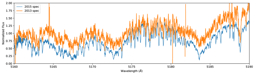
Figure 11: Comparison between the 2013 spectrum and 2015 median spectrum of KIC 1255 near the Mg I triplet. The two are consistent within the larger noise of the 2013 data.

4.4 Comparison to BOSZ

We first evaluate stellar parameters by comparing the high resolving power ($R=100,000$) BOSZ grids of ATLAS-APOGEE ATLAS9 models (Bohlin et al., 2017) to the median spectrum from 2015. Because the discrepancies in the literature are mostly differences in the surface gravity (see Table 2), we study the gravity-sensitive Mg triplet near 517 nm. The $R=100,000$ models are convolved with a Gaussian kernel that has a standard deviation $\sigma_{K}=\lambda/161,000\approx 0.03\AA$ to best match the data. This was slightly broader than we expected from combining inverse resolving powers in quadrature, which would imply that an $R_{expected}=75,000$ kernel convolved with an $R=100,000$ spectrum would result in a $R=60,000$ spectrum.

We start by comparing the measured spectrum with two BOSZ models in Figure 12. Here, the two BOSZ models are broadly representative of the two types of results in Table 2 (log(g)=4.5 and log(g)=4.0). The higher gravity log(g)=4.5 model appears to match the data better in terms of line ratios but does not explain all of the line depths in the spectrum.

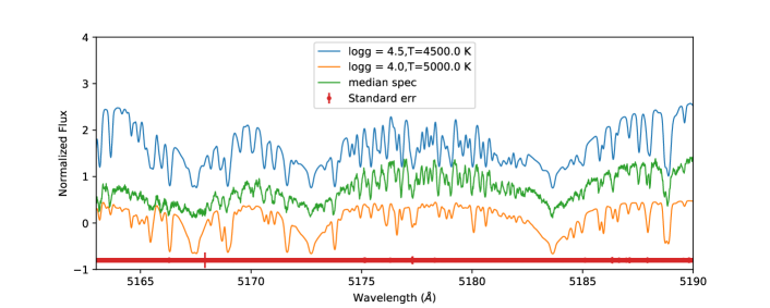
Figure 12: Median spectrum of KIC 1255 (Masuda et al., 2018) near the Mg triplet (green) compared to 4500 K BOSZ models with two different log(g)s (blue and orange). The standard error in the mean is shown at an arbitrary Y location as a red line.

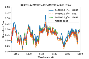
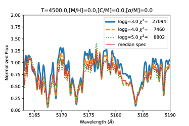
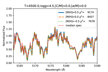
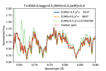
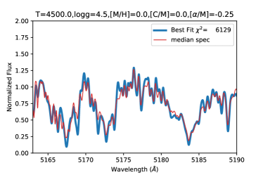
Figure 13: The BOSZ models are explored over the parameter space to search for a best fit as well as visualize how much each parameter affects the spectrum. The bottom right plot shows the best-fit BOSZ model, but it still under-predicts and over-predicts some line strengths.

We explore the 5 parameters in the BOSZ models: T_eff, log(g), [M/H], [$\alpha$/M] and [C/M] to constrain these parameters in KIC 1255. The sensitivity to each parameter for the BOSZ models are shown in Figure 13. For each parameter, we change the models by about 2 steps in the BOSZ grid. For a quantitative measure of the goodness-of-fit, we calculate a $\chi^{2}$ over the Mg triplet lines from 5160 to 5190 $\AA$. The errors are estimated from the standard deviation of the spectra over the night.

After initial constraints on the models from the sensitivity to parameters search, we downloaded a grid of BOSZ models with effective temperatures ranging from 4250 K to 4750 K, Log(g) from 4.0 to 4.5, [M/H] from 0.0 to 0.5, [C/M]=0.0 and [$\alpha$/M] = -0.25 to 0.0. We found the model with the $\chi^{2}$ statistic over the Mg I triplet lines from 5160 to 5190 $\AA$. The minimum $\chi^{2}$ model for this entire grid is the same as shown in Figure 13 on the Bottom Right: T_eff=4500 K, Log(g)=4.5, [M/H]=0.0, [C/M]=0.0, $\alpha=-0.25$. This is similar to the log(g)$\approx$4.6, T_eff=4500 stellar parameters derived from photometry and low resolution spectroscopy listed in Table 2.

4.5 SpecMatch-Emp

We also use the open-source SpecMatch-Emp tool (Yee et al., 2017) to estimate the stellar parameters using the Subaru spectrum. SpecMatch-Emp uses a library of Keck HIRES spectra to match the spectrum and derive stellar parameters. We cut the default HIRES library and Subaru spectra to the wavelengths from 5000 $\AA$ to 5900 $\AA$, which includes the gravity-sensitive Mg I triplet.

Figure 14 shows the chi-squared differences between the median Subaru spectrum and the models. The effective temperature and radius parameters show clear global $\chi^{2}$ minima for the HIRES spectral libraries. However, the metallicity is less well constrained. The resulting best-fit parameters from SpecMatch-Emp are T_eff=4440 K $\pm$ 70 K, [Fe/H]=-0.08$\pm$0.09, log(g)=4.63$\pm$0.12, R=0.69 $\pm$ 0.10 R_⊙ and Mass=0.70 $\pm 0.08~{}$M_⊙. Figure 15 shows the linear combination of spectra that best-fit KIC 1255 from SpecMatch-Emp over a subset of the wavelengths near the Mg I triplet.

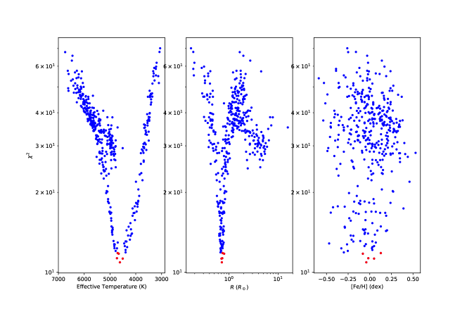
Figure 14: $\chi^{2}$ as a function of stellar parameters found by SpecMatch-Emp. The effective temperature and radii show clear global minima.

We summarize these SpecMatch-Emp and BOSZ results in Table 2, which both favor a main-sequence log(g) $\approx$ 4.6 star. Our analysis of the median 2015 spectrum therefore indicates that the stellar spectrum shows no strong contamination from planet disintegration activity . Unfortunately, this makes diagnosing the gaseous material evaporating from sublimated dust grains challenging to detect. A brighter transiting disintegrating system may reveal itself more strongly, if discovered in the TESS field.

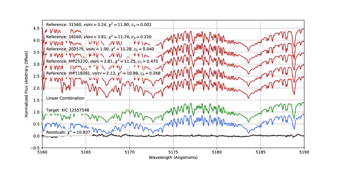
Figure 15: Linear combination of templates that best matches KIC 1255 near the Mg I triplet.

We posit that the initial analysis of the 2013 Subaru spectrum (Kawahara et al., 2013) that found a temperature and log(g) of 4950 K and 3.9 log(cm/s^-2) was affected by insufficient signal to noise in the spectrum. The 2013 data has a 30% smaller count rate (in e^-/s) than the 2015 data likely because the 2013 weather and guiding were sub-optimal. On top of that, the total exposure time for the 2013 observations was only 1.5 hours. The consequence of the increased noise in the 2013 spectra affected the interpretation of this high resolution spectrum. For example, the SNR of the Na D lines was $\sim$ 30, which is near the threshold needed for the Takeda et al. (2005) equivalent width method employed in the initial analysis. We therefore conclude that the noise in the spectrum affected the stellar parameters rather than gas absorption from sublimating dust grains.

5 Conclusions

We obtained ground-based R band photometry from the Kuiper 61-inch telescope to follow up a possible slowdown in disintegration activity observed in 2013 and 2014. Schlawin et al. (2016) found shallow transits that were all below the Kepler observatory average in August-September 2013 and August-September 2014. One possibility was a long term evolution of the disintegration activity, such as a reduction of available dusty material of the planet or a slowdown in the disintegration mechanism. Our transit depths from June-July 2016 are instead consistent with the depths from the Kepler observatory from 2009 to 2013, with a KS-test between the two distributions resulting in a p-value of 0.5 that depths are drawn from the same distribution. This indicates that the shallow transit depths observed in August-September 2013 and August-September 2014 likely fell into the 14-36 day long quiescent intervals of disintegration activity as observed in Kepler photometry (Kawahara et al., 2013; van Werkhoven et al., 2014; Croll et al., 2015).

We re-analyzed the existing Kepler photometry with PCA to better understand the time dependence and statistics of the light curves. We found that the first eigenvector corresponds to the overall transit depth whereas the second eigenvector corresponds to models of forward-scattering from large-sized dust grains. The first principal component tracks closely with the transit depths and exhibits modulations at periods of 22.9, 153 and 750 days. The second principal component is nearly sinusoidal with a 491 day period, indicating possible long term evolution of the dust particle sizes. The 22.9 day period matches the rotation period of the host star, which has previously been used to tie disintegration to stellar activity (Kawahara et al., 2013) or occultations of star spots (Croll et al., 2015). The remaining periodicities are longer than the dynamical and sublimation times of the planet and grains, so a different mechanism would be required to modulate the activity over these timescales.

van Lieshout et al. (2016) compiled the stellar parameters reported in the literature via photometric and spectroscopic methods and note that the high resolution spectrum show that KIC 1255 has the gravity of a sub-giant, whereas all other methods find that it is a main sequence star. One exciting possibility suggested in van Lieshout et al. (2016) is that the planet disintegration affects the spectral lines of the star and affects the high resolution spectrum from Kawahara et al. (2013). We explore this possibility by examining archival Subaru HDS spectra of KIC 1255. We find that the high resolution spectra are consistent with previous photometry and spectroscopy and that the host star is on the main sequence with T_eff=4440 $\pm$ 70 K, log(g) = 4.63 $\pm$ 0.12, [Fe/H]=-0.08$\pm$0.09, R=0.69$\pm$0.10 R_⊙ and M=0.70 $\pm$0.08 M_⊙. Therefore, the optical depth of any gas sublimating off dust grains is too small to affect the high resolution spectrum. We argue that low signal to noise in the initial Subaru HDS spectra affected previous interpretations of the stellar parameters.

6 Acknowledgements

The authors thank to Kento Masuda for sharing the 2015 Subaru spectrum of KIC 1255 and giving helpful comments on this work. Funding for E Schlawin is provided by NASA Goddard Spaceflight Center. The authors thank Saul Rappaport for helpful comments. The results reported herein benefited from collaborations and/or information exchange within NASA?s Nexus for Exoplanet System Science (NExSS) research coordination network sponsored by NASA?s Science Mission Directorate.

References

- Astropy Collaboration et al. (2013) Astropy Collaboration, Robitaille, T. P., Tollerud, E. J., et al. 2013, A&A, 558, A33 [ADS]
- Barnes et al. (2013) Barnes, J. W., van Eyken, J. C., Jackson, B. K., Ciardi, D. R., & Fortney, J. J. 2013, ApJ, 774, 53 [ADS]
- Berdyugina (2005) Berdyugina, S. V. 2005, Living Reviews in Solar Physics, 2, 8 [ADS]
- Bochinski et al. (2015) Bochinski, J. J., Haswell, C. A., Marsh, T. R., Dhillon, V. S., & Littlefair, S. P. 2015, ApJ, 800, L21 [ADS]
- Bodman & Quillen (2016) Bodman, E. H. L., & Quillen, A. 2016, ApJ, 819, L34 [ADS]
- Bohlin et al. (2017) Bohlin, R. C., Mészáros, S., Fleming, S. W., et al. 2017, AJ, 153, 234 [ADS]
- Boyajian et al. (2016) Boyajian, T. S., LaCourse, D. M., Rappaport, S. A., et al. 2016, MNRAS, 457, 3988 [ADS]
- Bradley et al. (2016) Bradley, L., Sipocz, B., Robitaille, T., et al. 2016, astropy/photutils: v0.3, doi:10.5281/zenodo.164986 [LINK]
- Brogi et al. (2012) Brogi, M., Keller, C. U., de Juan Ovelar, M., et al. 2012, A&A, 545, L5 [ADS]
- Brown et al. (2011) Brown, T. M., Latham, D. W., Everett, M. E., & Esquerdo, G. A. 2011, AJ, 142, 112 [ADS]
- Budaj (2013) Budaj, J. 2013, A&A, 557, A72 [ADS]
- Cardelli et al. (1989) Cardelli, J. A., Clayton, G. C., & Mathis, J. S. 1989, ApJ, 345, 245 [ADS]
- Castelli & Kurucz (2004) Castelli, F., & Kurucz, R. L. 2004, ArXiv Astrophysics e-prints, astro-ph/0405087 [ADS]
- Craig et al. (2015) Craig, M. W., Crawford, S. M., Deil, C., et al. 2015, ccdproc: CCD data reduction software, Astrophysics Source Code Library, ascl:1510.007 [ADS]
- Croll et al. (2015) Croll, B., Rappaport, S., & Levine, A. M. 2015, MNRAS, 449, 1408 [ADS]
- Croll et al. (2014) Croll, B., Rappaport, S., DeVore, J., et al. 2014, ApJ, 786, 100 [ADS]
- David et al. (2017) David, T. J., Petigura, E. A., Hillenbrand, L. A., et al. 2017, ApJ, 835, 168 [ADS]
- Foreman-Mackey et al. (2013) Foreman-Mackey, D., Hogg, D. W., Lang, D., & Goodman, J. 2013, PASP, 125, 306 [ADS]
- Gaia Collaboration et al. (2016) Gaia Collaboration, Prusti, T., de Bruijne, J. H. J., et al. 2016, A&A, 595, A1 [ADS]
- Gaia Collaboration et al. (2018) Gaia Collaboration, Brown, A. G. A., Vallenari, A., et al. 2018, A&A, 616, A1 [ADS]
- Gary et al. (2017) Gary, B. L., Rappaport, S., Kaye, T. G., Alonso, R., & Hambschs, F.-J. 2017, MNRAS, 465, 3267 [ADS]
- Gulbis et al. (2011) Gulbis, A. A. S., Bus, S. J., Elliot, J. L., et al. 2011, PASP, 123, 461 [ADS]
- Huber et al. (2014) Huber, D., Silva Aguirre, V., Matthews, J. M., et al. 2014, ApJS, 211, 2 [ADS]
- Jolliffe (2002) Jolliffe, I. 2002, Principal Component Analysis, Springer Series in Statistics (Springer) [LINK]
- Kawahara et al. (2013) Kawahara, H., Hirano, T., Kurosaki, K., Ito, Y., & Ikoma, M. 2013, ApJ, 776, L6 [ADS]
- Kite et al. (2016) Kite, E. S., Fegley, Jr., B., Schaefer, L., & Gaidos, E. 2016, ApJ, 828, 80 [ADS]
- Lim et al. (2015) Lim, P. L., Diaz, R. I., & Laidler, V. 2015, PySynphot User’s Guide, http://ssb.stsci.edu/pysynphot/docs/
- Luri et al. (2018) Luri, X., Brown, A. G. A., Sarro, L. M., et al. 2018, A&A, 616, A9 [ADS]
- Masuda et al. (2018) Masuda, K., Hirano, T., Kawahara, H., & Sato, B. 2018, Research Notes of the American Astronomical Society, 2, 50 [ADS]
- McQuillan et al. (2014) McQuillan, A., Mazeh, T., & Aigrain, S. 2014, ApJS, 211, 24 [ADS]
- Morton et al. (2016) Morton, T. D., Bryson, S. T., Coughlin, J. L., et al. 2016, ApJ, 822, 86 [ADS]
- Noguchi et al. (2002) Noguchi, K., Aoki, W., Kawanomoto, S., et al. 2002, PASJ, 54, 855 [ADS]
- Ochsenbein et al. (2000) Ochsenbein, F., Bauer, P., & Marcout, J. 2000, Astronomy and Astrophysics Supplement Series, 143, 23 [ADS]
- Osterbrock et al. (1996) Osterbrock, D. E., Fulbright, J. P., Martel, A. R., et al. 1996, PASP, 108, 277 [ADS]
- Pedregosa et al. (2011) Pedregosa, F., Varoquaux, G., Gramfort, A., et al. 2011, Journal of Machine Learning Research, 12, 2825
- Perez-Becker & Chiang (2013) Perez-Becker, D., & Chiang, E. 2013, MNRAS, 433, 2294 [ADS]
- Rackham et al. (2018a) Rackham, B. V., Apai, D., & Giampapa, M. S. 2018a, ApJ, 853, 122 [ADS]
- Rackham et al. (2018b) —. 2018b, AAS Journals, Submitted
- Rappaport et al. (2014) Rappaport, S., Barclay, T., DeVore, J., et al. 2014, ApJ, 784, 40 [ADS]
- Rappaport et al. (2018a) Rappaport, S., Gary, B. L., Vanderburg, A., et al. 2018a, MNRAS, 474, 933 [ADS]
- Rappaport et al. (2012) Rappaport, S., Levine, A., Chiang, E., et al. 2012, ApJ, 752, 1 [ADS]
- Rappaport et al. (2018b) Rappaport, S., Vanderburg, A., Jacobs, T., et al. 2018b, MNRAS, 474, 1453 [ADS]
- Rayner et al. (2003) Rayner, J. T., Toomey, D. W., Onaka, P. M., et al. 2003, PASP, 115, 362 [ADS]
- Ridden-Harper et al. (2018) Ridden-Harper, A. R., Keller, C. U., Min, M., van Lieshout, R., & Snellen, I. A. G. 2018, ArXiv e-prints, arXiv:1807.07973 [ADS]
- Sanchis-Ojeda et al. (2015) Sanchis-Ojeda, R., Rappaport, S., Pallè, E., et al. 2015, ApJ, 812, 112 [ADS]
- Schlawin et al. (2016) Schlawin, E., Herter, T., Zhao, M., Teske, J. K., & Chen, H. 2016, ApJ, 826, 156 [ADS]
- Seager & Mallén-Ornelas (2003) Seager, S., & Mallén-Ornelas, G. 2003, ApJ, 585, 1038 [ADS]
- Stassun et al. (2017) Stassun, K. G., Collins, K. A., & Gaudi, B. S. 2017, AJ, 153, 136 [ADS]
- Stauffer et al. (2017) Stauffer, J., Collier Cameron, A., Jardine, M., et al. 2017, AJ, 153, 152 [ADS]
- Strassmeier (2009) Strassmeier, K. G. 2009, A&A Rev., 17, 251 [ADS]
- Takeda et al. (2005) Takeda, Y., Ohkubo, M., Sato, B., Kambe, E., & Sadakane, K. 2005, Publications of the Astronomical Society of Japan, 57, 27 [ADS]
- van Eyken et al. (2012) van Eyken, J. C., Ciardi, D. R., von Braun, K., et al. 2012, ApJ, 755, 42 [ADS]
- van Lieshout et al. (2014) van Lieshout, R., Min, M., & Dominik, C. 2014, A&A, 572, A76 [ADS]
- van Lieshout et al. (2016) van Lieshout, R., Min, M., Dominik, C., et al. 2016, A&A, 596, A32 [ADS]
- van Werkhoven et al. (2014) van Werkhoven, T. I. M., Brogi, M., Snellen, I. A. G., & Keller, C. U. 2014, A&A, 561, A3 [ADS]
- Vanderburg et al. (2015) Vanderburg, A., Johnson, J. A., Rappaport, S., et al. 2015, Nature, 526, 546 [ADS]
- Wright & Sigurdsson (2016) Wright, J. T., & Sigurdsson, S. 2016, ApJ, 829, L3 [ADS]
- Yee et al. (2017) Yee, S. W., Petigura, E. A., & von Braun, K. 2017, ApJ, 836, 77 [ADS]
- Yu et al. (2015) Yu, L., Winn, J. N., Gillon, M., et al. 2015, ApJ, 812, 48 [ADS]