${\bf H_{2}}$ self–shielding with non-LTE rovibrational populations: implications for cooling in protogalaxies

Abstract

The abundance of molecular hydrogen (${\rm H_{2}}$), the primary coolant in primordial gas, is critical for the thermodynamic evolution and star–formation histories in early protogalaxies. Determining the photodissociation rate of ${\rm H_{2}}$ by an incident Lyman-Werner (LW) flux is thus crucial, but prohibitively expensive to calculate on the fly in simulations. The rate is sensitive to the ${\rm H_{2}}$ rovibrational distribution, which in turn depends on the gas density, temperature, and incident LW radiation field. We use the publicly available cloudy package to model primordial gas clouds and compare exact photodissociation rate calculations to commonly–used fitting formulae. We find the fit from Wolcott-Green et al. (2011) is most accurate for moderate densities ${\rm n\sim 10^{3}cm^{-3}}$ and temperatures, $T\sim 10^{3}$K, and we provide a new fit, which captures the increase in the rate at higher densities and temperatures, owing to the increased excited rovibrational populations in this regime. Our new fit has typical errors of a few percent percent up to ${\rm n\leq 10^{7}~{}cm^{-3}}$, ${\rm T\leq 8000}$K, and ${\rm H_{2}}$ column density ${\rm N_{H2}\leq 10^{17}~{}cm^{-2}}$, and can be easily utilized in simulations. We also show that pumping of the excited rovibrational states of ${\rm H_{2}}$ by a strong LW flux further modifies the level populations when the gas density is low, and noticeably decreases self-shielding for $J_{21}>10^{3}$ and ${\rm n<10^{2}cm^{-3}}$. This may lower the “critical flux” at which primordial gas remains ${\rm H_{2}}$–poor in some protogalaxies, enabling massive black hole seed formation.

1 Introduction

It has long been known that the cooling of metal–free primordial gas, from which the first generation of stars form in protogalaxies, is dominated by ${\rm H_{2}}$ molecules (Saslaw & Zipoy, 1967). Once these first (“Population III”) stars begin to shine, however, the UV radiation they emit begins to photodissociate ${\rm H_{2}}$ via the Lyman–Werner (LW) bands (${\rm E_{\nu}=11.1-13.6eV})$. Photodissociation feedback is non–trivial to model, particularly when the ${\rm H_{2}}$–column density becomes sufficiently high for it to become self–shielding (${\rm N_{H_{2}}}\mathrel{\hbox to0.0pt{\lower 4.0pt\hbox{\hskip 1.0pt$\sim$}\hss}\raise 1.0pt\hbox{$>$}}10^{13}{\rm cm}^{-2})$. Accurate modeling is important because the thermodynamic and star formation histories in early protogalaxies depend sensitively on the ${\rm H_{2}}$ abundance.

An example of this sensitivity occurs in the well–known “direct collapse” scenario, in which a protogalaxy may avoid fragmentation (and thereby Pop III star formation) if exposed to a sufficiently strong UV flux from a near neighbor (e.g. Regan et al., 2017, and references therein). In this case, the ${\rm H_{2}}$–abundance remains too low to cool below the virial temperature of the halo, preventing fragmentation on stellar scales. It has been proposed that the resulting rapid accretion possible in this scenario may lead to the formation of massive black holes (${\rm M_{BH}\mathrel{\hbox to0.0pt{\lower 4.0pt\hbox{\hskip 1.0pt$\sim$}\hss}\raise 1.0pt\hbox{$>$}}10^{4-5}M_{\odot}}$) that seed the earliest quasars (see reviews by Volonteri, 2010; Haiman, 2013; Wise, 2018). The predicted “critical” UV–flux to keep protogalactic [gas ${\rm H_{2}}$–poor (commonly denoted $J_{\rm crit}$) depends sensitively on the detailed calculation of the optically–thick ${\rm H_{2}}$–photodissociation rate.

Calculating the full optically–thick photodissociation rate on the fly is prohibitively expensive in simulations due to the large number of LW transitions. There are a total of 301 rovibrational states of the ground electronic state (X) and over half a million allowed electronic transitions. Previous studies have relied, therefore, on fitting formulae for the optically–thick ${\rm H_{2}}$ photodissociation rate provided by Draine & Bertoldi (1996). Their fit models the behavior well when primarily the ground (ortho and para) states of the molecule are populated, Alternatively, some studies use the modifed fit provided by Wolcott-Green et al. (2011, hereafter WGHB11), which is more accurate at higher densities and temperatures, when the rotational levels of the ground vibrational state are in, or close to, LTE.

Both of these approximations are gross simplifications of the true rovibrational level populations, which in general are time-dependent and sensitive to the gas density, temperature, and rate of UV excitation. As discussed in WGHB11, the optically–thick rate can be quite sensitive to changes in the level populations, and in particular to the number of states that contribute to self–shielding, as more states becoming signficantly populated reduces the effective self–shielding column density.

In this paper, we use the publicly available cloudy package (Ferland et al., 2017) to calculate the ${\rm H_{2}}$ rovibrational populations under conditions similar to those in a pristine protogalactic gas cloud irradiated by UV. We compare the resulting optically–thick photodissociation rate to that predicted by the commonly used fitting formulae. We find that the fitting formula provided by WGHB11 is accurate in a narrow range of densities and temperatures (${\rm n\approx 10^{3}cm^{-3}}$ and a few$\times 10^{3}$K), and we provide an improved fitting formula that is accurate for a larger swath of the parameter space. In particular, our improved fit matches the true rate of only a few percent up to $T=8000$K, ${\rm n=10^{7}~{}cm^{-3}}$, ${\rm N_{H2}=10^{16}~{}cm^{-2}}$, and with typical errors of order ten per cent up to higher column density, ${\rm N_{H2}=10^{17}~{}cm^{-2}}$.

In the case of a protogalactic candidate for direct collapse, there is an additional modfication to the rovibrational distribution and thus to the optically–thick ${\rm H_{2}}$– photodissociation rate that may be important, and which has not been considered in this context previously. When irradiated in the UV, decays following electronic excitation populate excited rovibrational levels of the ground electronic state (X), which subsequently decay through infrared emission in a radiative cascade. In the presence of a very strong UV flux, the radiative cascade of the UV–pumped ${\rm H_{2}}$ molecules can be interrupted by absorption of another UV photon. Shull (1978) found this “re-pumping” affects the radiative cascade $J_{21}\mathrel{\hbox to0.0pt{\lower 4.0pt\hbox{\hskip 1.0pt$\sim$}\hss}\raise 1.0pt\hbox{$>$}}10^{3}$, and is more likely than decay of the molecule to a lower rovibrational state when the incident UV flux exceeds $J_{21}\sim 10^{5}$, with $J_{21}$ defined in the usual way: $J_{\nu}=J_{21}\times 10^{-21}{\rm~{}erg~{}s^{-1}~{}cm^{-2}~{}sr^{-1}~{}Hz^{-1}}$.

We find in our cloudy models that pumping from excited rovibrational states, leading to reduced effective column density, can decrease self–shielding by up to an order of magnitude at fluxes as low as $J_{21}=$ a few $\times 10^{3}$ when the density is low ${\rm n<10^{3}~{}cm^{-3}}$. Importantly, this is similar to the common determinations of $J_{\rm crit,21}\sim 10^{3}$ (e.g. WGHB11). At higher densities ($>10^{3}~{}{\rm cm^{-3}}$), the rovibrational level populations tend toward their LTE values and we find there is no effect on the self–shielding behavior even for the strongest UV flux we consider, $J_{21}\sim 10^{5}$.

This paper is organised as follows: In § 2 we describe the details of our numerical modeling; in § 3 we discuss our results using a variety of cloudy models, and an updated fitting formulae for the optically–thick ${\rm H_{2}}$ photodissociation rate. We summarize our results and offer conclusions in § 4.

2 Numerical Modeling

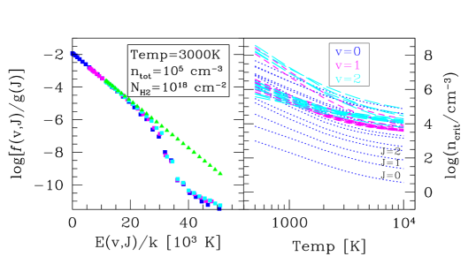
Figure 1: Left The fractional populations of ${\rm H_{2}}$ in rovibrational states with ${\rm v=0-2}$ and energy ${\rm E_{v,J}}$ predicted by the cloudy “Large ${\rm H_{2}}$” model. Green triangles show the LTE populations while the resolved (non–LTE) populations in ${\rm v=0,1,2}$ are shown by dark blue, magenta, and cyan squares, respectively. Right: The temperature dependence of the critical density (for LTE) is shown for each of the states ${\rm v=(0-2),J}$ (with dotted, short–dash, and long–dash lines, respectively.) As illustrated in this panel, $T=3,000$K, ${\rm n=10^{5}~{}cm^{-3}}$ exceeds the critical density of the lowest $\sim 35$ states, and the populations of these states, shown in the left–hand panel, are indeed near their LTE values, as expected.

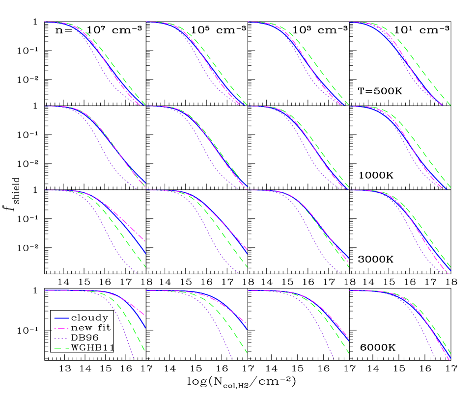
Figure 2: The optically–thick ${\rm H_{2}}$–photodissociation rate is shown, parameterized by the self–shielding factor, ${\it f}_{\rm shield}(N_{H2},T)=k{\rm{}_{LW}(N_{H2},T)/{\it k}{{}_{LW}(N_{H2}=0,T)}}$. Dark blue (solid) curves show results with fully–resolved rovibrational populations from cloudy models (at fixed density and temperature, as indicated on the figure). Green (dashed) and purple (dotted) curves show the fitting formulae for $f_{\rm sh}$ provided by Wolcott-Green et al. (2011) and Draine & Bertoldi (1996), respectively. Magenta (dot-dash) curves show results of the more accurate revised fitting formula in Equations 7-LABEL:Eq:NewAlpha.

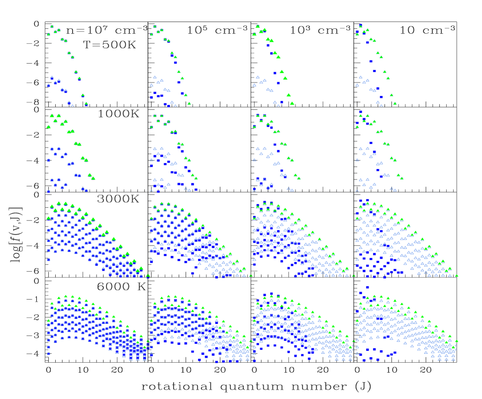
Figure 3: The fractional populations of ${\rm H_{2}}$ in our cloudy models are shown for each rovibrational state (v¡5,J). Dark blue squares are used for the fully–resolved (non-LTE) results while grey (open) triangles are the full LTE populations. Green (filled) triangles show a Boltzmann distribution for populations in the ground vibrational state only ${\rm v=0}$, which was the basis for a commonly used fitting formulas for $f_{\rm shield}$ provided by Wolcott-Green et al. (2011).

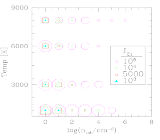
Figure 4: The densities and temperatures of cloudy models in which the a strong UV flux increases the optically–thick ${\rm H_{2}}$ photodissociation rate by more than a threshold factor $x$ are shown for three threshold values $x=1.25,2,10$ with small, medium, and large (circles) respectively. Results with four UV–intensities are shown, as indicated in the figure legend.

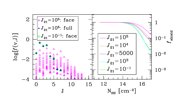
Figure 5: Left: The fractional population of ${\rm H_{2}}$ in rovibrational states (v,J) are shown for two different cloudy models with the same temperature (${\rm T=6000}$K) and density (${\rm n=1~{}cm^{-3}}$). Blue (filled) triangles show the cumulative populations of a cloud with ${\rm N_{H2}=10^{17}~{}cm^{-2}}$and irradiated by a strong–UV flux ($J_{21}=10^{5}$, in the usual units). Magenta (open) triangles show only the populations at the illuminated face of the same cloud. Green (open) circles show the populations at the face of a cloud irradiated by a much weaker UV flux ($J_{21}=0.1$). The panel shows that significant UV–pumping of excited rovibrational states occurs at the illuminated face, while the populations deeper in the cloud are unaffected by the strong incident UV flux. Right: the optically–thick photodissociation rate, parameterized by a shield factor $f_{\rm shield}$, at varying UV flux levels (see legend). As expected for the strong–UV case ($J_{21}=10^{5}$), self–shielding is weaker due to pumping of ${\rm H_{2}}$ to a larger number of rovibrational states, while at $J_{21}=10^{3}$, the shielding is much closer to the “no–pumping”case ($J_{21}=0.1$). As in the left panel, the cloudy models have constant temperature ${\rm T=6000}$K and density ${\rm n=1~{}cm^{-3}}$.

2.1 Cloudy Models

We use the most recent version of the publicly available package cloudy (v17.01) to calculate the rovibrational level populations of ${\rm H_{2}}$ in a gas of primordial composition and illuminated on one face (plane parallel geometry). We use a grid of densities and temperatures in the range $n=10^{0-7}~{}{\rm cm^{-3}}$ and $T=500-10^{5}$K. We hold both constant in our models, in order to tease apart the effects on the rovibrational distribution and the resulting photodissociation rate.

We use the Draine & Bertoldi (1996) galactic background spectrum for the incident radiation in our fiducial models (see their Equation 23), but our results are not sensitive to this choice. If we use the Black & van Dishoeck (1987) interstellar radiation field instead, the photodisosciation is nearly unchanged. (However, neither of these spectra have prior processing in the LW bands; Wolcott-Green et al. 2017 show that if the incident radiation originates from an older stellar population, absorption lines in the spectrum can change the resulting photodissociation rate by a factor of two or more.)

We use the “large ${\rm H_{2}}$” model, details of which can be found in Shaw et al. (2005); this model resolves all 301 bound levels of the ${\rm H_{2}}$ electronic ground state and six excited electronic states. Several thousand energy levels of the molecule and approximately $5\times 10^{5}$ permitted transitions are included. In order to explore the results at high UV flux and low density, we decreased the threshold fractional abundance of ${\rm H_{2}}$ at which the resolved populations are calculated (“H2-to-H-limit” in cloudy) from its default ($10^{-8}$) to $10^{-12}$.

2.2 The Rate Calculation

Photodissociation of ${\rm H_{2}}$ occurs primarily via the two–step Solomon process, in which the molecule is first electronically pumped by a UV photon ($11.1-13.6$ eV) from the ground state ${\rm X}^{1}\Sigma^{+}_{g}$ to the ${\rm B}^{1}\Sigma^{+}_{u}$ (Lyman) or ${\rm C}^{1}\Pi_{u}$ (Werner) states. The subsequent decay to the vibrational continuum results in dissociation $\sim 15$ per cent of the time. The “pumping rate” from a given rovibrational state ($v,J$) to an excited electronic state ($v^{\prime},J^{\prime}$) is:

$$\zeta_{\it{v,J,v^{\prime},J^{\prime}}}=\int_{\it{\nu_{\rm th}}}^{\nu_{13.6~{}eV}}4\pi\sigma_{\nu}\frac{J_{\nu}}{h_{\rm P}\nu}{\rm d}\nu,$$ (1)

where $\sigma_{\nu}$ is the frequency dependent cross–section and $h_{\rm P}$ is Plank’s constant. The frequency threshold, $\nu_{\rm th}$, corresponds to the lowest energy photons capable of efficiently dissociating ${\rm H_{2}}$, with $h\nu=11.18$ eV. We do not include photons with energies above the Lyman limit, which are likely to have been absorbed by the neutral IGM at the relevant redshifts (prior to reionization). In the direct collapse scenario with irradiation from a bright neighbor, the escape fraction of ionizing photons may be small anyway (see e.g. Wise et al., 2014). Including ${\rm E>13.6}$eV radiation would cause increased hydrogen ionization in the collapsing gas, which is not included in the present context.

The dissociation rate from a given ($v,J$) is the product of the pumping rate and the fraction of decays that result in dissociation (summed over all excited states, $v^{\prime},J^{\prime}$):

$$k_{{\rm diss},v,J}=\sum_{\it v^{\prime},J^{\prime}}\zeta_{\it v,J,v^{\prime},J^{\prime}}{\it f}_{{\rm diss},v^{\prime},J^{\prime}}.$$ (2)

The dissociation probabilities $f_{{\rm diss},v^{\prime},J^{\prime}}$, are provided by Abgrall et al. 2000.

While cloudy outputs the optically–thick dissociation rate itself, we re–calculate the rate in order to remove the effect of HI shielding ${\rm H_{2}}$ and isolate the self–shielding only. This also allows us to test the effects of changing one variable at a time, including the incident spectrum, the rovibrational distribution, and the temperature. WGHB11 found that the total shielding of ${\rm H_{2}}$ can be modeled with good accuracy by including a simple multiplcative factor that depends only on the HI column density: $f_{\rm shield,tot}{\rm(N_{H2},N_{HI},T)}=f_{\rm shield}{\rm(N_{H2})}\times f_{\rm HI(N_{HI})}$. Therefore, the effects we quantify for self–shielding are directly applicable to the total shielding, though HI is not included in our fiducial calculations.

We initiate the calculation with the cloudy incident spectrum at the irradiated face, and step through each discrete zone, summing the contributions to the frequency–dependent optical depth from the ${\rm H_{2}}$ transitions. In each zone, we use the resolved rovibrational populations from cloudy, ${\it f}_{v,J}$. The total rate in a given zone is then:

$$k_{\rm diss}=\sum_{\it v,J}k_{{\rm diss},{\it v,J}}\times{\it f}_{v,J}$$ (3)

2.3 Critical Densities for LTE in ${\bf H_{2}}$ Rovibrational States

One of the primary challenges in calculating the optically–thick photodissociation rate of ${\rm H_{2}}$ is determining the rovibrational level population distribution. In the non-LTE case, the distribution is time-dependent and sensitive to the gas temperature, density, as well as the UV pumping rate.

In a low–density gas, collisional de-excitation is slow and the radiative decay rates entirely determine the cascade to lower states; however, the radiative lifetimes are long enough that even at moderate densities collisional de-excitation begins to have an effect (Draine, 2010). The lowest energy states (${\rm v=0,J}$) reach LTE at critical densities of ${\rm n_{H}\mathrel{\hbox to0.0pt{\lower 4.0pt\hbox{\hskip 1.0pt$\sim$}\hss}\raise 1.0pt\hbox{$<$}}10~{}cm^{-3}}$ at ${\rm T=10^{4}K}$ (see Figure 1). The critical density for a given transition is:

$$n_{c}\left(u\rightarrow l\right)=\frac{A\left(u\rightarrow l\right)}{\gamma\left(u\rightarrow l\right)}$$ (4)

here $\gamma\left(u\rightarrow l\right)$ is the collisional de-excitation rate and ${A\left(u\rightarrow l\right)}$ is the spontaneous decay transition probability. Above the critical density, the fractional population of the state approaches its LTE value and is then dependent only on the temperature. Because ${\rm A\left(u\rightarrow l\right)\propto E_{lu}^{5}}$ (where ${\rm E_{lu}}$ is the energy of the transition between upper and lower states), the critical density increases rapidly with J within a vibrational manifold while it decreases rapidly with temperature. Figure 1 shows the temperature dependence of the critical densities of the lowest energy levels (${\rm v=0-2}$,J). We use the fitting formulae for the collisional rates provided by Le Bourlot et al. (1999), which do not include all of the highest energy levels, but are nonetheless useful for the present purpose.

The left panel of Figure 1 shows the ${\rm H_{2}}$ fractional level populations (${\rm v=0-2}$,J) determined by cloudy for a gas at T$=3000$K and ${\rm n=10^{5}~{}cm^{-3}}$. Resolved (non–LTE) populations (squares) diverge from the LTE values (triangles) for states with energies above ${\rm E_{v,J}/k_{B}\sim 2\times 10^{4}}$K, for which the critical densities exceed ${\rm n=10^{5}~{}cm^{-3}}$. In the right panel of this figure, we show the temperature dependence of the critical density for the same states ${\rm v=(0-2),J}$. From this figure, we see that the critical densities of the lowest $\sim 35$ states are less than ${\rm n=10^{5}~{}cm^{-3}}$ at ${\rm T=3000}$K, and the populations of these states (shown in the left panel) are indeed near their LTE values, as expected.

2.4 Analytical Fitting Formulae for the Shielding Factor

Because of the computational expense of calculating the full optically–thick ${\rm H_{2}}$–photodissociation rate, several analytic fits have been suggested, parameterized by a “shielding factor:”

$$f_{\rm shield}{\rm(N_{H2},T)}=k_{\rm diss}{\rm(N_{H2},T)}/k_{\rm diss}{\rm(N_{H2}=0,T)}.$$ (5)

Draine & Bertoldi (1996) (hereafter DB96) provided two useful fitting formulae for this purpose, the more accurate of which (their equation 37) has the form:

$$f_{\rm shield,DB}\left(N_{\rm H_{2}},T\right)=\frac{0.965}{\left(1+x/b_{5}\right)^{\alpha}}+\frac{0.035}{\left(1+x\right)^{0.5}}\\ \times\exp\left[-8.5\times 10^{-4}\left(1+x\right)^{0.5}\right].$$ (6)

DB96 set $\alpha=2,x\equiv N_{\rm H_{2}}/5\times 10^{14}~{}{\rm cm^{-2}}$, $b_{5}\equiv b/10^{5}~{}{\rm cm~{}s^{-1}}$, where $b$ is the Doppler broadening parameter.

WGBH11 showed that this fit is only accurate for low-density gas at temperatures of $\sim$a few hundred K. They modified it by setting $\alpha=1.1$ in order to better fit the population results in gas at $\sim$a few thousand Kelvin and densities $\sim 10^{3}{\rm cm^{-3}}$– relevant for a gravitationally– collapsing protogalactic halo. With this modification, self–shielding is weaker than the original DB96, appropriate for ${\rm H_{2}}$ populations that are spread out over more (v,J) states, as explained above.

3 Results and Discussion

3.1 How accurate are fitting formulae for $\it{f_{shield}}$?

With our cloudy models, we can evaluate the accuracy of the DB96 and WGHB11 fits compared to the “true” photodissociation rate over a wide swath of the parameter space. We include higher denities (${\rm n\leq 10^{7}cm^{-3}}$) and temperatures (${\rm T\leq 8000}$K) than in those previous studies, so that we can quantify the changes in the rate when the excited vibrational states become populated and eventually reach LTE. WGHB11 considered gas with density up to only ${\rm n\mathrel{\hbox to0.0pt{\lower 4.0pt\hbox{\hskip 1.0pt$\sim$}\hss}\raise 1.0pt\hbox{$<$}}10^{3}~{}cm^{-3}}$, and the DB96 fits were designed for much lower temperatures, ${\rm T\sim 100}$K.

In Figure 2 we show our $f_{\rm shield}$ results in cloudy models with low flux $J_{21}=0.1$ (dark blue curves). The DB96 fitting formula (gray curves) significantly overestimates shielding compared to cloudy at all but the lowest temperatures and densities (${\rm T=500K,n=10~{}cm^{-3}}$), as expected. The WGHB11 fit (green dashed curves) is more accurate up to higher temperature and density ${\rm T\approx 3000K}$, ${\rm n\approx 10^{3}~{}cm^{-3}}$); however, it also gives $f_{\rm shield}$ that is far too small (underestimates the actual photodissociation rate) at ${\rm T>3000K}$, ${\rm n>10^{3}~{}cm^{-3}}$. While this regime may not be relevant for the direct–collapse scenario, in which the gas thermodynamic evolution is determined at lower density ${\rm n\sim 10^{2}}$, it could be important for simulations of “Pop III” star formation in the presence of a strong incident UV flux.

Figure 3 shows the origin of the discrepancy of the WGHB11 fit. The resolved level populations for each of the cloudy models (dark blue squares) are shown in comparison to the predicted LTE populations (light blue triangles). The WGHB11 fit was based on a Boltzmann distribution only in the ground vibrational state, shown in the figure by green triangles. This $v=0$ model is a good approximation up to ${\rm T\sim 3000}$K. At higher temperatures and densities, however, the populations in $v>0$ states increase. Because the number of populated states is what matters for $f_{\rm shield}$ – a greater number of populated states leads to lower effective column density for shielding – the $v=0$ assumption for $f_{\rm shield}$ is erroneously small.

3.2 A New Fitting Formula for $\it{f_{\rm shield}}$

In order to find a more accurate fitting formula for $f_{\rm shield}$, we need to increase the sensitivity to temperature for densities above ${\rm n>10~{}cm^{-3}}$, reflecting the strong temperature dependence of the critical densities.

We make use of the original form provided by DB96, which WGHB11 modified with a new factor $\alpha$. Here, we introduce a density and temperature dependence of $\alpha$, so that the effect of spreading populations over more levels at high n/T is captured:

$$f_{\rm shield}\left(N_{\rm H_{2}},T\right)=\frac{0.965}{\left(1+x/b_{5}\right)^{\alpha(n,T)}}+\frac{0.035}{\left(1+x\right)^{0.5}}\\ \times\exp\left[-8.5\times 10^{-4}\left(1+x\right)^{0.5}\right].$$ (7)

$$\alpha{\rm\left(n,T\right)=A_{1}(T)\times dexp\left(-c_{1}\times log\left(n/cm^{-3}\right)\right)+A_{2}(T)}\\ {\rm A_{1}(T)=c_{2}\times log\left(T/K\right)-c_{3}}\\ {\rm A_{2}(T)=-c_{4}\times log\left(T/K\right)+c_{5}}\\$$ (8)

The best fit parameters, optimized using the amoeba routine in Numerical Recipes (Press et al., 1993), are as follows: $c_{1}=0.2856,~{}c_{2}=0.8711,~{}c_{3}=1.928,~{}c_{4}=0.9639,~{}c_{5}=3.892$. The accuracy of the new fit is improved over the entire parameter space compared to the previous fits, as shown in Figure 2, with typical errors of a few percent for $f_{\rm shield}$ up to ${\rm N_{H2}=10^{17}~{}cm^{-2}}$.

It is worth noting that Richings et al. (2014) also used cloudy models similar to ours to investigate the accuracy of various fitting formulae compared to the “true” optically–thick rate. However, in that study, the true rate is calculated by cloudy itself, which includes HI–shielding of ${\rm H_{2}}$ along with self–shielding. Therefore, their results are particular to those cloudy models and their specific HI/${\rm H_{2}}$ profiles. As a result, we have not compared our results to the fitting formula they provide.

3.3 Is pumping important at the relevant flux strength?

In order to quantify the effect of a strong incident UV flux on the optically–thick ${\rm H_{2}}$–photodissociation rate in a primordial cloud, we have run a grid of cloudy models with a range of flux intensities, $J_{21}=\left(0.1,10^{5}\right)$, gas temperatures, ${\rm T=(500,8000)K}$, and densities ${\rm n=10^{0-7}~{}cm^{-3}}$. In Figure 4 we show the combinations for which a strong flux changes the shielding by more than a threshold factor $f_{\rm shield}\left(J_{21}\right)/f_{\rm shield}\left(J_{21}=0.1\right)>x$, for three threshold values $x=1.25,2,10$. Our results are shown if the above criterion is fulfilled at any column density up to ${\rm N_{H2}=10^{17}~{}cm^{-2}}$.

In the majority of cases, there is no signficant change in the self-shielding except at very high intensity, $J_{21}=10^{5}$. However, at low densities ${\rm n\leq 10^{2}~{}cm^{-3}}$, even a “moderate” UV intensity increases the dissociation rate, For example, an incident flux of only $J_{21}=5,000$ reduces shielding by a factor $>2$ for a gas ${\rm n=10~{}cm^{-3}}$ and by more than an order of magnitude when ${\rm n=1~{}cm^{-3}}$. Even a flux of just $J_{21}=10^{3}$ leads to a $40-50$ per cent decrease in the shielding in the lowest density cases ${\rm n\leq 10~{}cm^{-3}}$.

Why is there a pronounced difference in self–shielding in the low–density, high–flux cases? Figure 5 shows the origin of this effect. The fractional populations of the ${\rm H_{2}}$ rovibrational levels are shown, in the left–hand panel in both the strong– and weak–UV cases, for a low density cloudy model (${\rm n=10~{}cm^{-3}}$). Because pumping has the greatest effect near the edge of the cloud, where there is the least shielding, we show the level populations at the irradiated face. In the strong–UV case (magenta open triangles), many excited states ${\rm v>0}$ populated. This is to be expected for a low–density gas, wherein strong UV pumping leads to a radiative cascade through excited states that are not populated by collisional processes alone. In contrast, in the weak–UV case, (green circles) only a few states are populated. We also show the cumulative populations (blue filled triangles) in the strong–UV case, which are nearly identical to those with weak–UV. This illustrates that pumping does not affect the bulk populations, as is expected due to shielding.

As discussed above, the spreading out of ${\rm H_{2}}$ column density in more (v,J) states by pumping decreases the effective self–shielding column density, since each molecule “sees” fewer molecules in the same (v,J) state between it and the irradiated face of the cloud. The right panel of Figure 5 shows the “pumped” shielding factor $f_{\rm shield}$ ($J_{21}=5,000$) is three times larger than for small $J_{21}$ at $N{\rm{}_{H2}=10^{17}~{}cm^{-2}}$. With $J_{21}=10^{5}$, the optically–thick photodissociation rate is $\sim$ an order of magnitude larger than the same for small $J_{21}$. At $J_{21}=10^{3}$, the largest change in the shield factor is $\sim 40$ per cent at ${\rm N_{H2}}\sim$ a few $\times 10^{15}{\rm cm^{-3}}$. In both panels of Figure 5, all of the cloudy models have constant ${\rm T=6000}$K and ${\rm n=1~{}cm^{-3}}$.

In higher density models, ${\rm n>10^{3}~{}cm^{-3}}$, there is no pumping effect on the ${\rm H_{2}}$ rovibrational populations. This is because the populations in the first few vibrational states (the most important for self–shielding) are already tending toward (or in) LTE at these densities (see Figure 3). In addition, larger neutral hydrogen column densities likely decrease the UV pumping more in these higher density cases, even near the illuminated face of the cloud.

It is worth noting that the density/temperature/$J_{21}$ space where pumping modifies the self–shielding behavior is very similar to that relevant for determining the critical flux to keep the halo ${\rm H_{2}}$–poor, and thus for potential direct collapse to a supermassive–black hole seed. For example, Omukai (2001); Shang et al. (2010), show that the bifurcation in the cooling history of DCBH candidate halos occurs when collapsing gas reaches ${\rm n\sim 10^{2}~{}cm^{-3}}$ and ${\rm T=8000}$K and the critical flux is $J_{21}\sim 10^{3-4}$ (WGBH11 and references therein). Therefore, it is likely that weaker shielding caused by UV–pumping at densities ${\rm n=10^{0-2}~{}cm^{-3}}$ is indeed relevant in the direct–collapse case, and pumping may well lead to a smaller $J_{\rm crit}$ if accounted for in simulations.

4 Conclusions

Using cloudy non-LTE models of pristine gas, we calculate the optically–thick ${\rm H_{2}}$ photodissociation rate using the resolved level populations and compare to the fitting formulae most commonly used in simulations. We find that the formula provided by Wolcott-Green et al. (2011) is most accurate at moderate densities, $n\mathrel{\hbox to0.0pt{\lower 4.0pt\hbox{\hskip 1.0pt$\sim$}\hss}\raise 1.0pt\hbox{$<$}}10^{3}~{}{\rm cm^{-3}}$, but fails to capture the weakening of shielding at higher densities and temperatures, when the populations in ${\rm v>0}$ tend to LTE. We provide a new modification to the fitting formula that increases its accuracy at all densities and temperatures and is a good fit up to ${\rm n\sim 10^{7}~{}{\rm cm^{-3}}}$, T$=8000$K, ${\rm N_{H2}=10^{17}~{}cm^{-2}}$. This new analytical fit can be easily used in simulations and one–zone models to better approximate the optically–thick photodissociation rate.

We also find that the photodissociation rate can be significantly increased in the presence of a strong UV flux, $J_{21}\mathrel{\hbox to0.0pt{\lower 4.0pt\hbox{\hskip 1.0pt$\sim$}\hss}\raise 1.0pt\hbox{$>$}}$ a few $\times 10^{3}$ due to pumping of molecules to excited rovibrational states. Increasing the number of populated states decreases the effective self–shielding column density that each molecule “sees,” and thus increases the optically–thick rate. This effect occurs only in gas at relatively low densities, ${\rm n\leq 10^{2}~{}{\rm cm^{-3}}}$, which happen to be similar to those important for the determination of $J_{\rm crit}$ for direct–collapse black hole formation. We find shielding is decreased by as much as an order of magnitude in some cases for an incident flux $J_{21}\sim 10^{4}$, and even a flux as low as $J_{21}\sim 10^{4}$ can cause a change $>40$ per cent in some cases.

References

- Abgrall et al. (2000) Abgrall H., Roueff E., Drira I., 2000, A&AS, 141, 297
- Black & van Dishoeck (1987) Black J. H., van Dishoeck E. F., 1987, ApJ, 322, 412
- Draine (2010) Draine B., 2010, in Physics of the Interstellar and Intergalactic Medium Molecular Hydrogen. pp 346–351
- Draine & Bertoldi (1996) Draine B. T., Bertoldi F., 1996, ApJ, 468, 269
- Ferland et al. (2017) Ferland G. J., Chatzikos M., Guzmán F., Lykins M. L., van Hoof P. A. M., Williams R. J. R., Abel N. P., Badnell N. R., Keenan F. P., Porter R. L., Stancil P. C., 2017, Rev. Mex. Astron. Astrofis, 53, 385
- Haiman (2013) Haiman Z., 2013, in Wiklind T., Mobasher B., Bromm V., eds, Astrophysics and Space Science Library Vol. 396 of Astrophysics and Space Science Library, The Formation of the First Massive Black Holes. p. 293
- Le Bourlot et al. (1999) Le Bourlot J., Pineau des Forêts G., Flower D. R., 1999, MNRAS, 305, 802
- Omukai (2001) Omukai K., 2001, ApJ, 546, 635
- Press et al. (1993) Press W. H., Teukolsky S. A., Vetterling W. T., Flannery B. P., Lloyd C., Rees P., 1993, The Observatory, 113, 214
- Regan et al. (2017) Regan J. A., Visbal E., Wise J. H., Haiman Z., Johansson P. H., Bryan G. L., 2017, Nature Astronomy, 1, 0075
- Richings et al. (2014) Richings A. J., Schaye J., Oppenheimer B. D., 2014, MNRAS, 442, 2780
- Saslaw & Zipoy (1967) Saslaw W. C., Zipoy D., 1967, Nature, 216, 976
- Shang et al. (2010) Shang C., Bryan G. L., Haiman Z., 2010, MNRAS, 402, 1249
- Shaw et al. (2005) Shaw G., Ferland G. J., Abel N. P., Stancil P. C., van Hoof P. A. M., 2005, ApJ, 624, 794
- Shull (1978) Shull J. M., 1978, ApJ, 219, 877
- Volonteri (2010) Volonteri M., 2010, Nature, 466, 1049
- Wise (2018) Wise J. H., 2018, ArXiv e-prints
- Wise et al. (2014) Wise J. H., Demchenko V. G., Halicek M. T., Norman M. L., Turk M. J., Abel T., Smith B. D., 2014, MNRAS, 442, 2560
- Wolcott-Green et al. (2011) Wolcott-Green J., Haiman Z., Bryan G. L., 2011, MNRAS, 418, 838
- Wolcott-Green et al. (2017) Wolcott-Green J., Haiman Z., Bryan G. L., 2017, MNRAS, 469, 3329