Lattice quantum gravity with scalar fields
Abstract:
We consider the four-dimensional Euclidean dynamical triangulations lattice model of quantum gravity based on triangulations of . We couple it minimally to a scalar field in the quenched approximation. Our results suggest a multiplicative renormalization for the mass of the scalar field which is consistent with the shift symmetry of the discretized lattice action. We discuss the possibility of measuring the mass anomalous dimension and the gravitational binding energy between two scalar test particles, where a negative bound state energy would imply that this model has an attractive gravitational force.
1 Introduction
The problem of constructing a quantum theory of gravity in four dimensions is notoriously difficult because the theory is perturbatively non-renormalizable in four dimensions. However, it was conjectured by Weinberg in [1] that the quantum theory of gravity might be asymptotically safe in the ultraviolet (UV) by possessing an interacting fixed point with finite dimensional critical surface. There is no proof that this is true, but there is non-trivial evidence in its support ; see [2, 3] and references therein. However, there are arguments that argue that gravity cannot be described by a renormalizable quantum field theory in four dimensions based on the inconsistency between entropy scaling of black holes in the high-energy spectrum and that of a scale invariant theory [4, 5]. The argument goes that the entropy of a renormalizable theory must scale as . For gravity, the high-energy spectrum must be dominated by black holes. The black hole entropy area law tells us that . However, these scalings are consistent for the value , which curiously is also the value of the fractal (spectral) dimension obtained from lattice gravity simulations at short distances in both Euclidean dynamical triangulations (EDT) and Causal dynamical triangulations (CDT) [6, 7].
In this proceedings, we work under the assumption that there is merit in understanding gravity as a quantum field theory in four dimensions. In the 1990s, using the discretization of the Einstein-Hilbert action due to Regge, the phase diagram of dynamical triangulations was explored and it was hoped that one would find a second-order critical point, which could be identified as the asymptotically safe fixed point of Weinberg’s conjecture. This is crucial for the continuum extrapolation of the lattice model. However, the order of the phase transition turned out to be first-order [8, 9]. The approach we follow here introduces a non-trivial measure term which alters the structure of the phase diagram where it appears that the continuum limit can be taken.
2 Action and discretization
The Einstein-Hilbert action for a metric has the form,
| (1) |
where R is the Ricci scalar and and G are the cosmological constant and Newton’s constant respectively. On a triangulation, we discretize the volume according to
| (2) |
The Euclidean Einstein-Regge discrete action is given by :
| (3) |
where is the number of simplices of dimension , and are related to Newton’s constant and the cosmological constant . In our lattice simulations, must be tuned to a critical value such that an infinite lattice volume can be taken. This leaves two parameters in the theory, and . Note that for a fixed topology with fixed four-volume , the number of 0-simplices and 2-simplices i.e and are not independent but related by
where is the Euler characteristic. It is customary to start with the discrete Euclidean-Regge action [10]
| (4) |
where , and . Also, the volume of a d-simplex is given by :
| (5) |
Rewriting and above in terms of and and using the relation between them () and using Eq. (5), we can write Eq. (4) as,
| (6) |
Defining new variables and = , we recover the form written above in Eq. (3). The continuum path integral can be written as,
| (7) |
which we discretize by writing the grand canonical (i.e. volume can fluctuate) partition function as,
| (8) |
where is a symmetry factor which mods out the number of equivalent ways of labelling the vertices in a given triangulation . Note that the term in paranthesis is the contribution from a non-trivial measure term. It was shown [11] that this term is crucial in four dimensions unlike in lower dimensions. This term was absent in much of past work [12] which implicitly assumed triangulations. Another difference from what was done in the past is that we use degenerate triangulations [13] as opposed to the combinatorial ones used in [12]. The reason we employ degenerate triangulations is that it leads to a substantial reduction in finite-size effects compared to combinatorial triangulations.
3 Coupling to the scalar field
We introduce the scalar field as a matter field minimally coupled to gravity. In the continuum, the action coupled to the scalar field ignoring the self-interaction terms can be written as
| (9) |
where,
| (10) |
Here, is a test particle and the back reaction of the metric is ignored. The notion of distance is non-trivial to define on the lattice that itself is dynamical, but the geodesic distance can be understood via the propagation of massive particle as suggested in [14, 15] The propagator for the scalar field in a fixed background of constant curvature decays as,
| (11) |
where is the geodesic distance between two points. It is noted that , is the physical mass of the particle with multiplicative gravitational renormalization. The multiplicative renormalization follows from the shift symmetry of the discrete lattice action [16] and can be seen as follows,
| (12) | |||||
| (13) |
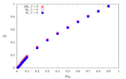
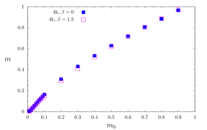
where is the simplex neighbor (or connectivity) matrix, is the bare mass and is the space-time dimension. For zero bare mass, there is a shift symmetry, , which implies that the renormalized mass should vanish in the limit that the bare mass is sent to zero.
4 Computation and results
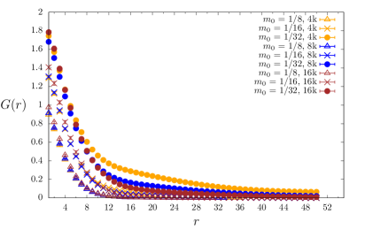
We restrict our analysis to the ensembles close to the critical line of the phase transition, where it was shown that the geometry has semi-classical properties, and on each degenerate dynamical triangulation, we calculate the propagator using,
| (14) |
The definition of the discrete Laplacian is given by,
| (15) |
Here, is the coordination number of a -simplex, which is 5 in our case. Unlike the combinatorial case studied in [12, 17], here we study degenerate triangulations. In such a setting, a given four-simplex can have non-unique neighbors. This enables us to construct the laplacian for configurations such that the sum of any particular row is just . In the limit of vanishing bare mass (), we have an exact zero mode of the operator corresponding to the zero eigenvalue of the Laplacian. It should be noted that there exists an alternate geometric description of the laplacian in terms of boundary () 111The action of on a given p-simplex yields an directed sum of (p - 1)-simplices on its boundary, whereas, yields directed sum of (p + 1)-simplices and co-boundary operators (). We can then write the laplacian as, , where we have used . See [18] for details and its role in gravitational systems coupled to fermions.
Similar to the continuum definition of the massive lattice scalar propagator, we can define the same quantity on the lattice as,
| (16) | |||||
| (17) |
where, is the renormalized mass. Unlike the previous study [12], we have not used smeared sources for the inversion of the matrix. However, it might be crucial for the future calculation of binding energy. In calculating the propagator over all configurations, we have considered five sources () per configuration and checked that our results are unaffected by this choice.
| Physical volume | ||||
|---|---|---|---|---|
| 1.47(10) | 1.5 | 0.5886 | 4000 | 0.054 |
| 1 | 0.0 | 1.669 | 4000 | 0.25 |
| 1 | 0.0 | 1.7024 | 8000 | 0.125 |
| 1 | 0.0 | 1.7325 | 16000 | 0.0625 |
4.1 Binding energy and Mass anomalous dimension of scalar fields
The calculation of the one-particle and two-particle propagators on generated ensembles can be fitted to the form as given below
| (18) | |||||
| (19) |
where is the energy of the two-particle state. The coefficient of the fits can then be used to calculate the binding energy associated as
| (20) |
such that at long distances, i.e. , the negative value of the binding energy, would represent an attractive force.
We now discuss the calculation of the mass anomalous dimension from a determination of the mass renormalization factor at the same physical volume but different lattice spacings. The bare and renormalized lagrangians are
| (21) |
| (22) |
Comparing them we get,
| (23) |
and,
| (24) |
Taking the log of ( 24) and then taking the derivative with respect to and identifying , we get:
| (25) |
where we have used the shorthand . Then, the mass anomalous dimension is given by,
| (26) |
In the future, we will explore additional volumes and lattice spacings and report on the results for gravitational binding energy and anomalous dimensions.
Acknowledgments: This research was supported by the US Department of Energy (DOE), Office of Science, Office of High Energy Physics, under Award Number DE-SC0009998.
References
- [1] S. Weinberg, “ULTRAVIOLET DIVERGENCES IN QUANTUM THEORIES OF GRAVITATION,” in General Relativity: An Einstein Centenary Survey, pp. 790–831. 1980.
- [2] D. F. Litim, “Fixed points of quantum gravity,” Phys. Rev. Lett. 92 (2004) 201301, arXiv:hep-th/0312114 [hep-th].
- [3] M. Niedermaier, “The Asymptotic safety scenario in quantum gravity: An Introduction,” Class. Quant. Grav. 24 (2007) R171–230, arXiv:gr-qc/0610018 [gr-qc].
- [4] O. Aharony and T. Banks, “Note on the quantum mechanics of M theory,” JHEP 03 (1999) 016, arXiv:hep-th/9812237 [hep-th].
- [5] A. Shomer, “A Pedagogical explanation for the non-renormalizability of gravity,” arXiv:0709.3555 [hep-th].
- [6] J. Laiho and D. Coumbe, “Evidence for Asymptotic Safety from Lattice Quantum Gravity,” Phys. Rev. Lett. 107 (2011) 161301, arXiv:1104.5505 [hep-lat].
- [7] D. N. Coumbe and J. Jurkiewicz, “Evidence for Asymptotic Safety from Dimensional Reduction in Causal Dynamical Triangulations,” JHEP 03 (2015) 151, arXiv:1411.7712 [hep-th].
- [8] P. Bialas, Z. Burda, A. Krzywicki, and B. Petersson, “Focusing on the fixed point of 4-D simplicial gravity,” Nucl. Phys. B472 (1996) 293–308, arXiv:hep-lat/9601024 [hep-lat].
- [9] B. V. de Bakker, “Further evidence that the transition of 4-D dynamical triangulation is first order,” Phys. Lett. B389 (1996) 238–242, arXiv:hep-lat/9603024 [hep-lat].
- [10] T. Regge, “GENERAL RELATIVITY WITHOUT COORDINATES,” Nuovo Cim. 19 (1961) 558–571.
- [11] B. Bruegmann and E. Marinari, “4-d simplicial quantum gravity with a nontrivial measure,” Phys. Rev. Lett. 70 (1993) 1908–1911, arXiv:hep-lat/9210002 [hep-lat].
- [12] B. V. de Bakker and J. Smit, “Gravitational binding in 4-D dynamical triangulation,” Nucl. Phys. B484 (1997) 476–494, arXiv:hep-lat/9604023 [hep-lat].
- [13] S. Bilke and G. Thorleifsson, “Simulating four-dimensional simplicial gravity using degenerate triangulations,” Phys. Rev. D59 (1999) 124008, arXiv:hep-lat/9810049 [hep-lat].
- [14] F. David, “What is the intrinsic geometry of two-dimensional quantum gravity?,” Nuclear Physics B 368 (Jan., 1992) 671–700.
- [15] H. W. Hamber and R. M. Williams, “Simplicial gravity coupled to scalar matter,” Nucl. Phys. B415 (1994) 463–496, arXiv:hep-th/9308099 [hep-th].
- [16] M. E. Agishtein and A. A. Migdal, “Critical behavior of dynamically triangulated quantum gravity in four-dimensions,” Nucl. Phys. B385 (1992) 395–412, arXiv:hep-lat/9204004 [hep-lat].
- [17] B. V. de Bakker and J. Smit, “Correlations and binding in 4-D dynamical triangulation,” Nucl. Phys. Proc. Suppl. 47 (1996) 613–616, arXiv:hep-lat/9510041 [hep-lat].
- [18] S. Catterall, J. Laiho, and J. Unmuth-Yockey, “Topological fermion condensates from anomalies,” JHEP 10 (2018) 013, arXiv:1806.07845 [hep-lat].
- [19] J. Laiho, S. Bassler, D. Coumbe, D. Du, and J. T. Neelakanta, “Lattice Quantum Gravity and Asymptotic Safety,” Phys. Rev. D96 no.~6, (2017) 064015, arXiv:1604.02745 [hep-th].