Most Probable Transition Pathways and Maximal Likely Trajectories in a Genetic Regulatory System

Abstract

We study the most probable transition pathways and maximal likely trajectories in a genetic regulation model of the transcription factor activator’s concentration evolution, with Gaussian noise and non-Gaussian stable Lévy noise in the synthesis reaction rate taking into account, respectively. We compute the most probable transition pathways by the Onsager-Machlup least action principle, and calculate the maximal likely trajectories by spatially maximizing the probability density of the system path, i.e., the solution of the associated nonlocal Fokker-Planck equation. We have observed the rare most probable transition pathways in the case of Gaussian noise, for certain noise intensity, evolution time scale and system parameters. We have especially studied the maximal likely trajectories starting at the low concentration metastable state, and examined whether they evolve to or near the high concentration metastable state (i.e., the likely transcription regime) for certain parameters, in order to gain insights into the transcription processes and the tipping time for the transcription likely to occur. This enables us: (i) to visualize the progress of concentration evolution (i.e., observe whether the system enters the transcription regime within a given time period); (ii) to predict or avoid certain transcriptions via selecting specific noise parameters in particular regions in the parameter space. Moreover, we have found some peculiar or counter-intuitive phenomena in this gene model system, including: (a) A smaller noise intensity may trigger the transcription process, while a larger noise intensity can not, under the same asymmetric Lévy noise. This phenomenon does not occur in the case of symmetric Lévy noise; (b) The symmetric Lévy motion always induces transition to high concentration, but certain asymmetric Lévy motions do not trigger the switch to transcription.

These findings provide insights for further experimental research, in order to achieve or to avoid specific gene transcriptions, with possible relevance for medical advances.

Key words: Most probable transition pathways; Maximal likely evolution trajectories; Brownian motion and Lévy motion; Nonlocal Fokker-Planck equation;  Onsager-Machlup action functional; Stochastic genetic regulation system

1 Introduction

Random fluctuations have been extensively considered in the modeling and analysis of genetic regulatory systems [1, 2, 3, 4, 5, 6]. These fluctuations may lead to switching between gene expression states [7, 8, 9, 10, 11, 12, 13]. To characterize this switching behaviour, researchers have been developing stochastic models [11, 12, 13, 14, 15] by taking noises into account in deterministic differential equations. Noisy fluctuations are mostly considered as Gaussian white noise in terms of Brownian motion [10, 11, 16, 17, 18]. But it has been observed that the transcriptions of DNA from genes and translations into proteins occur in a intermittent, bursty way [19, 20, 21, 22, 23]. This evolutionary manner [24, 25, 26, 27, 28, 29, 30] resembles the features of trajectories or solution paths of a stochastic differential equation with a Lévy motion. In contrast to the(Gaussian) Brownian motion, Lévy motion is a non-Gaussian process with heavy tails and occasional jumps.

For further information about noisy gene regulation, see [14, 17, 19, 20, 31, 32, 33, 34, 35, 36] and also [16, 37, 38, 39, 40].

In this present paper, we consider a genetic regulatory model for the evolution of the concentration for a transcription factor activator (TF-A), developed by Smolen et al.[41], with the synthesis reaction rate perturbed by stable Lévy fluctuations. Liu and Jia [11] investigated the effect of fluctuations arise from the Gaussian noise in the degradation and the synthesis reaction rate of the transcription factor activator, and found that a successive switch process occurred with the increase of the cross-correlation intensity between noises. In addition, Zheng et al. [13] used the mean first exit time and the first escape probability to examine the mean time scale and the likelihood for the concentration profile to evolve from low concentration regime to high concentration regime (indicating the transcription status).

Unlike the existing works in examining transition possibility and time scales under noises (e.g., [11, 13]), the objective of this present paper is to study the most probable transition pathways and maximal likely trajectories for concentration states themselves of the transcription factor activator (a protein) as time goes on. This offers the following information for the gene regulation system:
(i) The concentration transition pathways and evolution trajectories from low concentration to (or arriving near) high concentration, indicating the evolutionary routes to transcription.
(ii) The tipping time for the most probable transition pathways and maximal likely trajectories to pass the barrier between the low concentration state and the high concentration state.

To this end, we compute the most probable transition pathways (in the case of Gaussian noise), and the maximal likely trajectories (in the case of non-Gaussian noise) for this stochastic gene model, in order to gain insights into the concentration trajectories from the low concentration state to the high concentration state (i.e., the likely transcription regime), and the tipping time for these trajectories passing a threshold state between low and high concentration. Especially, we try to characterize the dependence of these dynamical behaviors on the noise parameters.

This paper is organized as follows. In Section 2, we introduce the TF-A monomer concentration model in a gene regulation system excited by a (Gaussian) Brownian motion and (non-Gaussian) Lévy motion, and propose our method on most probable transition pathways and maximal likely trajectories. In Section 3, we present the most probable transition pathways for the gene system under Gaussian noise. Further, we consider the maximal likely trajectories for the gene system with various non-Gaussian noise parameters, and examine which kind of noise is more beneficial for transcription. Finally, we summarize the above results in Section 4. The Appendix contains basic facts about a stable Lévy motion, and the nonlocal Fokker-Planck equation formulation for a stochastic differential equation with a stable Lévy motion.

2 Model and Method

We first introduce the TF-A monomer concentration model in a gene regulation system excited by the (Gaussian) Brownian motion and (non-Gaussian) stable Lévy motions, and then show most probable transition pathways for gene system under Gaussian noise and maximal likely trajectories.

2.1 Model: Stochastic gene regulation

We consider a model for the transcription factor activator (TF-A) of a genetic regulatory system, established by Smolen et al. [41]. A single transcriptional activator TF-A is considered as part of a pathway mediating a cellular response to a stimulus. The TF forms a homodimer bound to responsive elements (TF-REs). The TF-A gene incorporates one of these responsive elements, where binding to this element of homodimers will increase TF-A transcription. Only phosphorylated dimers can activate transcription. As shown in Fig 1(a), the phosphorylated (P) transcription factor activator (TF-A) activates transcription with a maximal rate $k_{f}$, with $k_{d}$ and $R_{bas}$ the degradation and synthesis rate of the TF-A monomer, respectively. The dissociation concentration of the TF-A dimer from TF-REs is denoted by $K_{d}$. Then the evolution of the TF-A concentration $x$ obeys the following differential equation [41]:

$$\dot{x}=\frac{k_{f}x^{2}}{x^{2}+K_{d}}-k_{d}x+R_{bas},$$ (1)

(a)

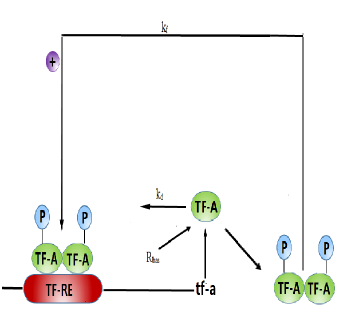
(b)

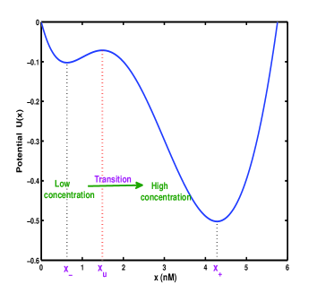
Fig 1: (a) Genetic regulatory model with a feedforward (Eq (1)); (b) The bistable potential $U$ for the TF-A monomer concentration model.

The system (1) can be rewritten as $\dot{x}=f(x)$, where $f(x)=\frac{k_{f}x^{2}}{x^{2}+K_{d}}-k_{d}x+R_{bas}$. The vector field $f(x)$ is also equal to $-U^{\prime}(x)$, with the potential function $U(x)=k_{f}\sqrt{K_{d}}\ \arctan\frac{x}{\sqrt{K_{d}}}+\frac{k_{d}}{2}x^{2}-(R_{bas}+k_{f})x$. This system has two stable states and one unstable state, when the parameters satisfy the condition: $[-(\frac{k_{f}+R_{bas}}{3k_{d}})^{3}+\frac{K_{d}(k_{f}+R_{bas})}{6k_{d}}-\frac{K_{d}R_{bas}}{2k_{d}}]^{2}+[\frac{K_{d}}{3}-(\frac{k_{f}+R_{bas}}{3k_{d}})^{2}]^{3}<0$. As in [11], we select suitable parameters: $k_{f}=6\;{\rm min}^{-1},~{}K_{d}=10,~{}k_{d}=1\;{\rm min}^{-1}$, and $R_{bas}=0.4\;{\rm min^{-1}}$. Then two stable states are $x_{-}\approx 0.62685\;{\rm nM}$ and $x_{+}\approx 4.28343\;{\rm nM}$ and the unstable state (a saddle point) is $x_{u}\approx 1.48971\;{\rm nM}$. See Fig 1(b).

The dynamical system (1) is a deterministic model. Some experiments indicated that basal synthesis rate $R_{bas}$ is influenced by random fluctuations arising from the biochemical reactions, the concentrations of other proteins, and gene mutations [24, 42, 11]. So as in [11], we consider the system (1) with Gaussian noise in terms of Brownian motion

$$\dot{X}_{t}=\frac{k_{f}X_{t}^{2}}{X_{t}^{2}+K_{d}}-k_{d}X_{t}+(R_{bas}+\epsilon\dot{B_{t}}),\qquad X_{0}=x_{0},$$ (2)

However, there exists powerful evidences indicating that gene expression with small diffusion and large bursting resembles the composition of systems with Lévy noise [24, 25, 26, 27]. Furthermore, some stochastic models of gene expression illustrate that transcriptional bursts display a heavily skewed distribution [24]. Zheng et al. [13] model random behaviour of the synthesis rate $R_{bas}$ on the genetic regulatory system (1) by a symmetric stable Lévy noise. But this symmetry is quite an idealized, special situation and does not have the property of the skewness. Hence, we take an asymmetric stable Lévy noise with skewness characteristic as a random perturbation of the synthesis rate $R_{bas}$. Then the model (1) becomes the following scalar stochastic gene regulation model with additive stable noise:

$$\dot{X}_{t}=\frac{k_{f}X_{t}^{2}}{X_{t}^{2}+K_{d}}-k_{d}X_{t}+(R_{bas}+\dot{\tilde{L_{t}}}^{\alpha,\beta}),\qquad X_{0}=x_{0},$$ (3)

where the scalar stable Lévy motion $\tilde{L_{t}}^{\alpha,\beta}$, with non-Gaussianity index $\alpha(0<\alpha<2)$, skewness index $\beta(-1\leq\beta\leq 1)$, scaling index $\sigma(\sigma>0)$ and shift index zero, is recalled in A1 Asymmetric stable Lévy motion $L_{t}^{\alpha,\beta}$ at the end of this paper. We denote $\epsilon\triangleq\sigma^{\alpha}$ the noise intensity. It is worth noting that we are concerned with the internal noise [43, 44], which can be realized as additive noise. In stochastic dynamical systems, it is customary to denote a system variable by a capital letter with time as subscript ($X_{t}$). A stable Lévy motion is asymmetric when $\beta\neq 0$ and symmetric when $\beta=0$. A solution orbit (also called a solution trajectory) $X_{t}$ has occasional (up to countable) jumps for almost all samples (i.e., realizations), except in the case with Brownian motion $B_{t}$ for which almost all the solution trajectories are continuous in time [45].

Without noise, the low concentration stable state $x_{-}$ and high concentration stable state $x_{+}$ are resilient (see Fig 1(b)): the TF-A concentration states will locally be attracted $x_{-}$ or $x_{+}$, as time increases for the deterministic system (1). It is known that stochastic fluctuations may induce switches between two stable states [41, 11]. The TF-A concentration, starting near the low concentration state $x_{-}$ in $D=(0,x_{u})$, arrives at a high concentration state (near $x_{+}$) by passing through the unstable saddle state $x_{u}$ (see Fig 1(b)). The threshold time instant when the system passes the unstable saddle state $x_{u}\approx 1.48971$ is called the ‘tipping time’ for a specific solution trajectory.

We now examine these system trajectories or orbits for the gene regulation model:
(i) How does the system evolve from low concentration (near $x_{-}$) to high concentration (near $x_{+}$), indicating the system in a transcription regime?
(ii) What is the tipping time while evolving from the low concentration state to the high concentration state?

2.2 Method

We first discuss the most probable transition pathways for the genetic system with (Gaussian) Brownian motion, and then consider the maximal likely trajectories for this system with (non-Gaussian) Lévy motion.

2.2.1 Most probable transition pathway

For the stochastic gene system (2) with Brownian motion, we obtain the most probable transition pathway [46] from the low concentration metastable state $x_{-}$ to the high concentration metastable state $x_{+}$, by minimizing the Onsager-Machlup action functional. This approach is not yet available for stochastic systems with Lévy motions. The most probable transition pathway $z_{m}(t)$ can be obtained by the least action principle

$$\delta\int_{0}^{T}OM(\dot{z},z)dt=0,$$ (4)

where the Onsager-Machlup function $OM(\dot{z},z)$ is defined by

$$OM(\dot{z},z)=\left(\frac{f(z)-\dot{z}}{\epsilon}\right)^{2}+f^{\prime}(z),$$ (5)

and the integral $\int_{0}^{T}OM(\dot{z},z)dt$ is called the Onsager-Machlup action functional. It needs to satisfy the Euler-Lagrange equation

$$\frac{d}{dt}\frac{\partial OM(\dot{z},z)}{\partial\dot{z}}=\frac{\partial OM(\dot{z},z)}{\partial z}$$ (6)

as the differential equation for $z_{m}(t)$. Hence, the most probable transition pathway $z_{m}(t)$ satisfies the following equation

$$\ddot{z}_{m}(t)=\frac{\epsilon^{2}}{2}f^{\prime\prime}(z_{m})+f^{\prime}(z_{m})f(z_{m}),~{}~{}~{}t\in(0,T),$$ (7)

$$z_{m}(0)=x_{-},~{}~{}z_{m}(T)=x_{+}.$$ (8)

Note that the Onsager-Machlup function given in (5) is convex in the variable $\dot{z}$. Thus, by Theorem 10 in Section 8.2.5 of [9, Page 481], if there exists a $C^{2}$ solution to the Euler-Lagrange equation, then it is indeed a (local) minimizer. We adopt a shooting method in [47] to numerically solve two-point boundary value problem (7)-(8). As this boundary value problem may not have a solution, the most probable transition pathway may not exist.

2.2.2 Maximal likely trajectory

The Onsager-Machlup action functional approach, in the previous subsection, for the most probable transition pathway is not yet available for stochastic systems with Lévy motions. Instead, we consider the maximal likely trajectory for the stochastic system (3) with non-Gaussian Lévy motion, starting at an initial state $x_{0}$ (but we will take it as the low concentration metastable state $x_{-}$). This is reminiscent of studying a deterministic dynamical system by examining the evolution of its trajectory starting from an initial state. Each sample solution path starting at this initial state is a possible outcome of the solution path $X_{t}$. What is the maximal likely trajectory of $X_{t}$? In order to answer the question, we need to decide on the maximal likely position $x_{m}(t)$ of the system (starting at the initial point $x_{0}$) at every given future time $t$, but this is the maximizer for the probability density function $p(x,t)\triangleq p(x,t;x_{0},0)$ of solution $X_{t}$. We first numerically solve the nonlocal Fokker-Planck equation (A.2), and then we find the maximal likely position $x_{m}(t)$ as the maximizer of $p(x,t)$ at every given time $t$. The probability density function $p(x,t)$ is a surface in the $(x,t,p)-$space. At a given time instant $t$, the maximizer $x_{m}(t)$ for $p(x,t)$ indicates the maximal likely location of this orbit at time $t$. The trajectory (or orbit) traced out by $x_{m}(t)$ is called the maximal likely trajectory starting at $x_{0}$. Thus, $x_{m}(t)$ follows the top ridge or plateau of the surface in the $(x,t,p)-$space as time goes on. Starting at every initial point, we may thus compute its maximal likely trajectory for the evolution of concentration for the transcription factor activator (and thus we occasionally call it the maximal likely evolution trajectory). The maximal likely trajectories [48, 49] are also called ‘paths of mode’ in climate dynamics and data assimilation [50, 51]. They may have jumps, as the solution sample paths of the stochastic system (3) have jumps due to Lévy motion.

As in [52], the maximal likely equilibrium state is defined as a state which either attracts or repels all nearby orbits. When it attracts all nearby orbits, it is called a maximal likely stable equilibrium state, while if it repels all nearby orbits, it is called a maximal likely unstable equilibrium state. Maximal likely equilibrium states depend on noise parameters $\alpha,\beta$, noise intensity $\epsilon$ as well as the genetic system parameters.

Fig 2 also shows one or two maximal likely equilibrium states. We observe that the maximal likely equilibrium state in high concentration is between $4$ and $5$, depending on $\alpha,\beta,\epsilon$, and it differs from the deterministic stable state $x_{+}\approx 4.28343$ due to the effect of noise.

(c)

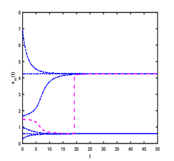
(d)

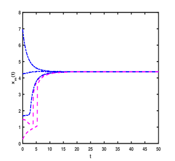
Fig 2: (Online color) Maximal likely evolution trajectories of stochastic system (3) starting at various initial concentration $x_{0}$. (a) With Lévy motion: $\alpha=1.5,\beta=0,\epsilon=0.02$. (b) With Lévy motion: $\alpha=1.5,\beta=0,\epsilon=0.4$.

In the following, we are especially interested in the maximal likely trajectories starting at the low concentration stable state $x_{-}\approx 0.62685$ and approaching (or arriving in a small neighborhood of) the maximal likely equilibrium stable state in the high concentration regime (more likely for transcription). Fig 2 also shows the maximal likely evolution trajectories for certain parameters. This definition of maximal likely evolution trajectories is based on maximizing the solution’s probability density at every time instant. We use a similar efficient numerical finite difference method developed by us in Gao et al. [53] to simulate the nonlocal Fokker-Planck equation (A.2). This applies to stochastic systems with finite as well as small noise intensity.

In summary, there are significant differences between most probable transition pathway and maximal likely trajectory. Firstly, the most probable transition pathway is a continuous trajectory from one metastable state to another metastable state. The maximal likely trajectory is a trajectory starting from one initial state. Secondly, the former is obtained via numerically solving the two-point boundary value problem (i.e., shooting method). The latter is calculated by solving an initial value problem. Thirdly, the former can be understood as the probability maximizer that sample solution paths lie within a tube with $z_{m}(t)$ as the center. The latter is determined by maximizing the probability density function (i.e., the solution of the Fokker-Planck equation) at every time instant.

3 Results

In the following section, we compute the most probable transition pathways and maximal likely evolution trajectories, in order to analyze how the TF-A concentration evolves from the low concentration state to the high concentration state. The most probable transition pathways $z_{m}(t)$ starting from $x_{-}\approx 0.62685$ and ending at $x_{+}\approx 4.28343$ and maximal likely trajectories $x_{m}(t)$ starting at $x_{-}\approx 0.62685$, are deterministic estimators as time goes on. The tipping time is the time needed (counting from the start) for this most probable transition pathways $z_{m}(t)$ and maximal likely evolution trajectories $x_{m}(t)$ to pass through the saddle point $x_{u}$. The tipping time for the most probable transition pathways and maximal likely evolution trajectories provides the threshold time instant at which the system enters the high concentration regime.

3.1 Gene regulation under Gaussian Brownian motion: Most probable transition pathway

For gene regulation system (2), we now examine the most probable transition pathway $z_{m}(t)$ starting at the low concentration metastable state $x_{-}\approx 0.62685$ and ending at the high concentration metastable state $x_{+}\approx 4.28343$. As seen in Fig 3, as time increases, for four different noise intensities $\epsilon=0.25,~{}0.5,~{}0.75,~{}1$, the most probable concentration increases to the high concentration quickly, and remains a nearly constant level (in transcription regime), then decreases to the high stable concentration state $x_{+}$ at $T=50$. Moreover, we clearly observe that the most probable concentration passes the ‘barrier’ $x_{u}\approx 1.48971$ faster for larger $\epsilon$. That is, the tipping time is shorter for larger noise intensity. The existence of such rare most probable transition pathways depends crucially on the system running time $T$, system parameters, and the noise intensity.

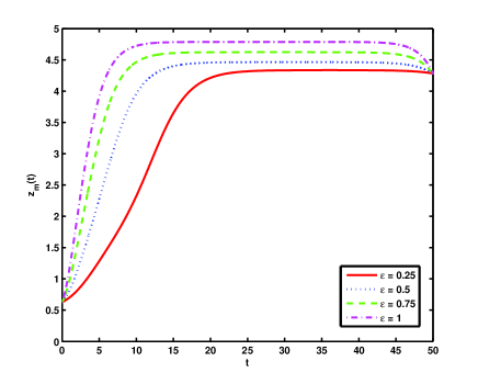
Fig 3: Most probable transition pathways $z_{m}(t)$ starting at the low concentration metastable state $x_{-}\approx 0.62685$ and ending at the high concentration metastable state $x_{+}\approx 4.28343$ under Gaussian noise with different noise intensities: $\epsilon=0.25,~{}0.5,~{}0.75,~{}1$.

3.2 Gene regulation under non-Gaussian Lévy motion: Maximal likely trajectory

For gene regulation system (3)with Lévy motion, the Onsager-Machlup action functional approach is not yet available. Therefore, we here focus on its maximal likely trajectories. We now investigate the influence of symmetric (see Fig 4(a)) and asymmetric (see Fig 4(b)) Lévy noise on maximal likely evolution trajectories. In Fig 4(a), as time increases, for four different noise intensities $\epsilon=0.25,~{}0.5,~{}0.75,~{}1$, the maximal likely concentration decreases a bit at the beginning, increases to the high concentration quickly, and finally remains a nearly constant level (in transcription regime). These dynamical behaviors, in the symmetric noise case, may appear intuitively correct, but this is not true in the asymmetric noise case as we now discuss.

In Fig 4(b), we notice that the maximal likely concentration goes through the saddle state $x_{u}$ and arrives at the high concentration state for smaller noise intensities $\epsilon=0.25,~{}0.5,~{}0.75$, but counter-intuitively decrease to a nearly constant low concentration for larger noise intensity $\epsilon=1$. In this work, we take time $t=50$ as the tipping time if the maximal likely concentration does not pass through the saddle point $x_{u}$ by time $t=50$. This suggests that the asymmetric Lévy noise with $\alpha=0.5,~{}\beta=-0.5$, and $\epsilon=1,~{}x_{0}=0.62685$, does not induce the switch mechanism for transcription.

(a)

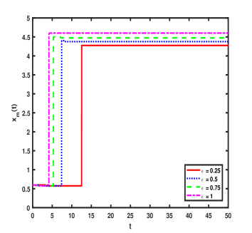
(b)

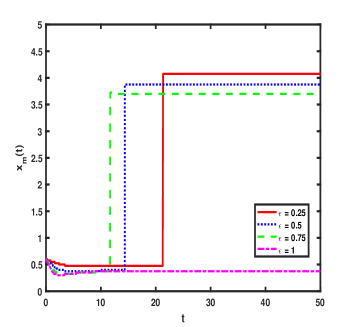
Fig 4: (Online color) Maximal likely evolution trajectories under symmetric ($\beta=0$) and asymmetric ($\beta\neq 0$) Lévy noise for various parameters. (a) Dependence on $\epsilon$: $\alpha=0.5,~{}\beta=0$. (b) Dependence on $\epsilon$: $\alpha=0.5,~{}\beta=-0.5$.

The reason for no possible transcription may be explained by the stability of two deterministic stable states $x_{-},~{}x_{+}$ in system (1), under the influence of noise. As shown in Fig 5(a), the state near $x_{-}$ is attracted to the maximal likely equilibrium stable state in high concentration domain and thus we have possible transcription for the smaller noise intensity $\epsilon=0.25$. But in Fig 5(b), the state near $x_{-}$ is attracted to the maximal likely equilibrium stable state in the low concentration state, and this offers an explanation for the counter-intuitive phenomenon of no possible transcription for the larger noise intensity $\epsilon=1$.

(a)

(b)

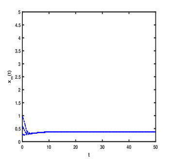
Fig 5: (Online color) Maximal likely evolution trajectories starting at various initial concentration $x_{0}$. (a) With Lévy motion: $\alpha=0.5,\beta=-0.5,\epsilon=0.25$. (b) With Lévy motion: $\alpha=0.5,\beta=-0.5,\epsilon=1$.

In summary, by examining the maximal likely trajectory starting from the low concentration metastable state $x_{-}$ , we have thus found that the symmetric ($\beta=0$) Lévy noise appears to induce transition to transcription, while asymmetric ($\beta\neq 0$) Lévy noise with certain parameters do not trigger the switch to transcription. Furthermore, we have explained the reason for no apparent transcription, due to the system stability change for some asymmetric stable Lévy noise. In the next subsection, we will further show effects of stable Lévy noise by computing the tipping time and the concentration values for maximal likely evolution trajectories at the end of computation ($t=50$).

3.3 Maximal likely transcription and tipping time

In this subsection, we investigate which kind of stable Lévy noise has a significant impact on the transcriptional activities, via the maximal likely concentration state value at $t=50$ (see Fig 6(a)) on the maximal likely evolution trajectories and the tipping time (see Fig 6(b)) for these trajectories.

(a)

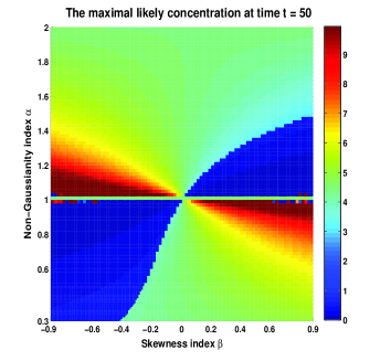
(b)

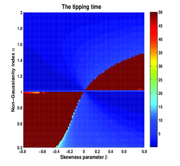
Fig 6: (Online color) The effects of noise parameters $\alpha,\beta$ on the maximal likely concentration and the tipping time. (a) The maximal likely concentration at $t=50$ with initial concentration $x_{0}=0.62685,~{}\epsilon=1$. (b) The tipping time for the maximal likely evolution trajectories with initial concentration $x_{0}=0.62685,~{}\epsilon=1$.

The red region in Fig 6(a) presents the valid transcription region corresponding to the gene regulation system with the noise within the parameter plane $(\beta,\alpha)$, as it shows the high concentration values (indicating transcription). Note that the symmetric ($\beta=0$) Lévy noise induces transition to transcription, but asymmetric ($\beta\neq 0$) Lévy noise with certain parameters do not trigger the switch to transcription.

The dark blue region indicates the situation with no transcription.

Likewise, as seen in Fig 6(b) about tipping time in the noise case in the parameter plane $(\beta,\alpha)$, the red region illustrates that no transcription has occurred by the time $t=50$ as there is no tipping from the low concentration to the high concentration state (i.e., the maximal likely trajectory does not pass through the saddle state $x_{u}$).

In addition, the critical line $\alpha=1$ helps form a part of the boundary between the transcription and no-transcription regions in the parameter plane. With this divided parameter plane, we can select combined parameters $\alpha$ and $\beta$, in order to achieve transcription within an appropriate time scale.

4 Conclusion

In this work, we have investigated the transcription factor activator’s concentration evolution in a prototypical gene regulation model, focusing on the effects of Gaussian Brownian noise and non-Gaussian Lévy noise in the synthesis reaction rate. We examine the most probable transition pathways under Gaussian noise and maximal likely trajectories under non-Gaussian noise, i.e., we visualize the trajectories from low concentration to high concentration. We also compute the tipping time from the low concentration state to (or arriving near) the high concentration state. The most probable transition pathways are computed by numerically solving a two-point boundary value problem. The maximal likely trajectories are calculated via numerically solving the nonlocal Fokker-Planck equation for the stochastic gene regulation model (3).

For a gene regulation system under Gaussian noise, we examine the most probable transition pathways $z_{m}(t)$ from the low concentration metastable state $x_{-}$ to the high concentration metastable state $x_{+}$, by minimizing the Onsager-Machlup action functional. For this same gene regulation system under non-Gaussian noise, the Onsager-Machlup least action principle is not yet available and we thus compute the maximal likely evolution trajectory $x_{m}(t)$ starting from the low concentration metastable state $x_{-}$. Both enable us to visualize the progress of the transcription factor activator’s concentration evolution as time goes on (i.e., observe whether the system enters the transcription regime).

We have indeed observed that the most probable transition pathway exists under Gaussian noise for certain evolution time scale and system parameters. Furthermore, we have characterized the concentration evolution with varying noise parameters: non-Gaussianity index $\alpha$, skewness index $\beta$ and noise intensity $\epsilon$. Therefore, we can predict the concentration level (or an appropriate transcription status) at a given future time, depending on the specific noise parameters in divided regions in the parameter plane (see Fig 6). We have also noticed some peculiar or counter-intuitive phenomena. For example, a smaller noise intensity may trigger the transcription process, while a larger noise intensity can not, in this gene system with the same asymmetric Lévy noise (see Fig 4(b) ). This phenomenon does not occur in the case of symmetric Lévy noise. Moreover, the symmetric ($\beta=0$) Lévy noise induces transition to transcription for all non-Gaussianity index $\alpha$, but asymmetric ($\beta\neq 0$) Lévy noise with certain non-Gaussianity index $\alpha$ do not trigger the switch to transcription.

These findings may provide helpful insights for further experimental research, in order to achieve or to avoid specific gene transcriptions.

Appendix

We recall the definition of a scalar stable Lévy motion $L_{t}^{\alpha,\beta}$ and the nonlocal Fokker-Planck equation for the probability density evolution of the solution to the stochastic system (3).

A1 Asymmetric stable Lévy motion $L_{t}^{\alpha,\beta}$

A scalar stable Lévy motion $L_{t}^{\alpha,\beta}$ is a stochastic process with the following properties [45, 48, 54, 55]:
(i) $L_{0}^{\alpha,\beta}=0$, almost surely (a.s.);
(ii) $L_{t}^{\alpha,\beta}$ has independent increments;
(iii)$L_{t}^{\alpha,\beta}$ has stationary increments: $L_{t}^{\alpha,\beta}-L_{s}^{\alpha,\beta}\sim S_{\alpha}((t-s)^{\frac{1}{\alpha}},\beta,0)$, for all $s$ and $t$ with $0\leq s\leq t$;
(iv) $L_{t}^{\alpha,\beta}$ has stochastically continuous sample paths, i.e., for every $s>0$, $L_{t}^{\alpha,\beta}\rightarrow L_{s}^{\alpha,\beta}$ in probability, as $t\rightarrow s$.

Here $S_{\alpha}(\sigma,\beta,\mu)$ is the so-called stable distribution [48, 55] and is determined by four indexes: non-Gaussianity index $\alpha(0<\alpha<2)$, skewness index $\beta(-1\leq\beta\leq 1)$, shift index $\mu(-\infty<\mu<+\infty)$ and scale index $\sigma(\sigma>0)$. A stable Lévy motion has jumps and its probability density function has heavy-tails (i.e., the tails decrease for large spatial variable like a power function [48, 54, 55]). The non-Gaussianity index $\alpha$ decides the thickness of the tail, as shown in Fig A.1(a). As seen in Fig A.1(b), the skewness index $\beta$ measures the asymmetry (i.e., non-symmetry) of the probability density function. The distribution is right-skewed if $\beta>0$, left-skewed if $\beta<0$, and symmetric for $\beta=0$ [48, 54, 55].

Especially, Brownian motion $B_{t}$ (corresponding to $\alpha=2,\beta=0$) has light tails (i.e., the tails decrease exponentially fast).

(a)

(b)

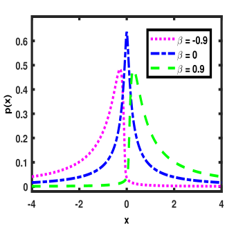
Fig A.1: (Online color) The probability density function $p(x)$ of $L_{t}^{\alpha,\beta}$ at time $t=1$. (a) Non-Gaussianity indexes $\alpha=0.4,~{}1.2,~{}2$ for $\beta=0$. (b) Skewness indexes $\beta=-0.9,~{}0,~{}0.9$ for $\alpha=0.5$.

A path for $L_{t}^{\alpha,\beta}$, although stochastically continuous, has occasional (up to countable) jumps for almost all samples (i.e., realizations), while almost all paths of Brownian motion $B_{t}$ are continuous in time. Figs A.2(a) and A.2(b) show two sample paths of $X_{t}$ for the stochastic gene regulation system (2) and (3), starting at low concentration state $x_{-}\approx 0.62685$. Unlike the phase portraits for deterministic dynamical systems [56, 57], these sample paths (‘orbit’ or ‘trajectories’) mingled together and can not provide much information. Most probable phase portraits [49, 48, 52] for the stochastic gene regulation system (3) is a powerful tool to understand the stochastic system.

(a)

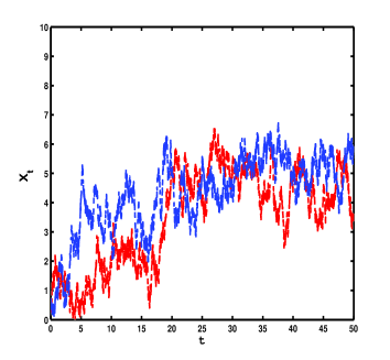
(b)

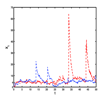
Fig A.2: (Online color) Two stochastic TF-A concentration sample paths $X_{t}$ starting at $X_{0}=x_{-}\approx 0.62685$ with noise intensity $\epsilon=1$.(a) Stochastic TF-A concentration sample paths $X_{t}$ with (Gaussian) Brownian motion. (b) Stochastic TF-A concentration sample paths $X_{t}$ with (non-Gaussian) Lévy motion at $\alpha=1.2,\beta=0$.

A2 Nonlocal Fokker-Planck equation

For the stochastic gene regulation system (3), let us recall the Fokker-Planck equation for the probability density function $p(x,t)\triangleq p(x,\!t;\;x_{0},\!0)$ of its solution $X_{t}$, with initial condition $X_{0}=x_{0}$. The generator $A$ for the solution process $X_{t}$ is ([41, 45, 48])

$$\begin{array}[]{l}Ap(x,t)=(f(x)+\epsilon M_{\alpha,\beta})\partial_{x}{p(x,t)}\\[8.61108pt] +\displaystyle\epsilon\int_{\mathbb{R}^{1}\backslash\{0\}}\left[p(x+y,t)-p(x,t)-I_{\{|y|<1\}}(y)y\partial_{x}{p(x,t)}\right]\nu_{\alpha,\beta}(dy),\end{array}$$ (A.1)

where $I$ is the indicator function and

$$M_{\alpha,\beta}=\left\{\begin{array}[]{ll}\frac{C_{1}-C_{2}}{1-\alpha},&\hbox{$\alpha\neq 1$,}\\ \left(\int_{1}^{\infty}{\frac{\sin(x)}{x^{2}}}dx+\int_{0}^{1}{\frac{\sin(x)-x}{x^{2}}}dx\right)\left(C_{2}-C_{1}\right),&\hbox{$\alpha=1$.}\end{array}\right.$$

Then the nonlocal Fokker-Planck equation for stochastic gene system (3) is

$$\frac{\partial}{\partial t}{p(x,t)}=A^{\ast}p(x,t),~{}~{}~{}~{}~{}p(x,0)=\delta(x-x_{0}),$$ (A.2)

where $A^{\ast}$ is the adjoint operator of $A$ and $\delta$ is the Dirac function. The adjoint operator $A^{\ast}$ can be further written as

$$\begin{array}[]{l}A^{\ast}p(x,t)=-{\partial}_{x}\left((f(x)+\epsilon M_{\alpha,\beta})p(x,t)\right)\\[8.61108pt] \displaystyle+\epsilon\int_{\mathbb{R}^{1}\backslash\{0\}}\left[p(x+y,t)-p(x,t)-I_{\{|y|<1\}}(y)y\partial_{x}p(x,t)\right]\nu_{\alpha,-\beta}(dy),\end{array}$$ (A.3)

where $\nu_{\alpha,\beta}(dy)=\frac{C_{1}I_{\{0<y<+\infty\}}(y)+C_{2}I_{\{-\infty<y<0\}}(y)}{\mid y\mid^{1+\alpha}}dy,$ $C_{1}=\frac{H_{\alpha}(1+\beta)}{2}$, $C_{2}=\frac{H_{\alpha}(1-\beta)}{2}.$ Here,

$$H_{\alpha}=\left\{\begin{array}[]{ll}\frac{\alpha(1-\alpha)}{\Gamma(2-\alpha)\cos(\frac{\pi\alpha}{2})},{}{}{}&\alpha\neq 1,\\ 2/\pi,{}{}{}&\alpha=1.\end{array}\right.$$

For a symmetric stable Lévy motion ($\beta=0$), the jump measure is $\nu_{\alpha,0}(dy)=\frac{H_{\alpha}}{2|y|^{1+\alpha}}dy$.

This nonlocal equation can be numerically solved by a similar finite difference method as in [53].

References

- 1. Raser, J. M., and O’Shea, E. K., “Noise in gene expression: origins, consequences, and control,” Science 309(5743), 2010-2013 (2005).
- 2. Maheshri, N., and O’Shea, E. K., “Living with noisy genes: how cells function reliably with inherent variability in gene expression,” Annu. Rev. Biophys. Biomolec. Struct. 36(36), 413-434 (2007).
- 3. Swain, P. S., Elowitz, M. B., and Siggia, E. D., “Intrinsic and extrinsic contributions to stochasticity in gene expression,” Proc. Natl. Acad. Sci. 99(20), 12795-12800 (2002).
- 4. Kittisopikul, M., and Süel, G. M., “Biological role of noise encoded in a genetic network motif,” Proc. Natl. Acad. Sci. 107(30), 13300-13305 (2010).
- 5. Bressloff, P. C., Stochastic Processes in Cell Biology (Springer, New York, 2014).
- 6. Süel, G. M., Kulkarni, R. P., Dworkin, J., Garcia-Ojalvo, J., and Elowitz, M. B., “Tunability and noise dependence in differentiation dynamics,” Science 315(5819), 1716-1719 (2017).
- 7. Turcotte, M., Garcia-Ojalvo, J., and Süel, G. M., “A genetic timer through noise-induced stabilization of an unstable state,” Proc. Natl. Acad. Sci. 105(41), 15732-15737 (2008).
- 8. Assaf, M., Roberts, E., and Luthey-Schulten, Z., “Determining the stability of genetic switches: explicitly accounting for mRNA noise,” Phys. Rev. Lett. 106(24), 248102 (2011).
- 9. Hasty, J., Pradines, J., Dolnik, M., and Collins, J. J., “Noise-based switches and amplifiers for gene expression,” Proc. Natl. Acad. Sci. 97(5), 2075-2080 (2000).
- 10. Hasty, J., Pradines, J., Dolnik, M., and Collins, J. J., “Stochastic regulation of gene expression,” Stochastic & Chaotic Dynamics in the Lakes: S. American Institute of Physics, 502, 191-196 (2000).
- 11. Liu, Q., and Jia, Y., “Fluctuations-induced switch in the gene transcriptional regulatory system,” Phys. Rev. E 70, 041907 (2004).
- 12. Xu, Y., Feng, J., Li, J., and Zhang, H., “Lévy noise induced switch in the gene transcriptional regulatory system,” Chaos 23(1), 013110 (2013).
- 13. Zheng, Y., Serdukova, L., Duan, J., and Kurths, J., “Transitions in a genetic transcriptional regulatory system under Lévy motion,” Sci. Rep. 6, 29274 (2016).
- 14. Augello, G., Valenti, D., and Spagnolo, B., “Non-Gaussian noise effects in the dynamics of a short overdamped Josephson junction,” Eur. Phys. J. B, 78:225-234 (2010).
- 15. Cognata, A. La, Valenti, D., Dubkov, A.A., and Spagnolo, B., “Dynamics of two competing species in the presence of Lévy noise sources,” Phys. Rev. E 82:011121 (2010).
- 16. Gui, R., Liu, Q., Yao, Y., Deng, H., Ma, C., Jia, Y., and Yi, M., “Noise decomposition principle in a coherent feed-forward transcriptional regulatory loop,” Front. Physiol. 7, 600 (2016).
- 17. Süel, G. M., Garcia-Ojalvo, J., Liberman, L. M., and Elowitz, M. B., “An excitable gene regulatory circuit induces transient cellular differentiation,” Nature 440(7083), 545-550 (2006).
- 18. Li, Y., Yi, M., and Zou, X., “The linear interplay of intrinsic and extrinsic noises ensures a high accuracy of cell fate selection in budding yeast,” Sci. Rep. 4(4), 5764 (2014).
- 19. Friedman, N., Cai, L., and Xie, X. S., “Linking stochastic dynamics to population distribution: an analytical framework of gene expression,” Phys. Rev. Lett. 97(16), 168302 (2006).
- 20. Lin, Y. T., and Doering, C. R., “Gene expression dynamics with stochastic bursts: construction and exact results for a coarse-grained model,” Phys. Rev. E 93(2), 022409 (2016).
- 21. Holloway, D. M., and Spirov, A. V., “Transcriptional bursting in drosophila development: stochastic dynamics of eve stripe 2 expression,” PLoS One 12(4), e0176228 (2017).
- 22. Kumar, N., Singh, A., and Kulkarni, R. V., “Transcriptional bursting in gene expression: analytical results for general stochastic models,” PLoS Comput. Biol. 11(10), e1004292 (2015).
- 23. Dar, R. D., Razooky, B. S., Singh, A., Trimeloni, T. V., McCollum, J. M., Cox, C. D., Simpson, M. L., and Weinberger, L. S., “Transcriptional burst frequency and burst size are equally modulated across the human genome,” Proc. Natl. Acad. Sci. 109(43), 17454-17459 (2012).
- 24. Raj, A., Peskin, C., Tranchina, D., Vargas, D., and Tyagi, S., “Stochastic mRNA synthesis in mammalian cells,” PLoS Biol. 4, 1707 (2006).
- 25. Golding, I., Paulsson, J., Zawilski, S. M., and Cox, E. C., “Real-time kinetics of gene activity in individual bacteria,” Cell 123(6), 1025-1036 (2005).
- 26. Bohrer, C. H., and Roberts, E. A., “Biophysical model of supercoiling dependent transcription predicts a structural aspect to gene regulation” BMC Biophys. 9(1), 1-13 (2016).
- 27. Muramoto, T., Cannon, D., Gierlinski, M., Corrigan, A., Barton, G. J., and Chubb, J. R., “Live imaging of nascent RNA dynamics reveals distinct types of transcriptional pulse regulation,” Proc. Natl. Acad. Sci. 109(19), 7350-7355 (2012).
- 28. Dubkov, A.A., Cognata, A. La, and Spagnolo, B., “The problem of analytical calculation of barrier crossing characteristics for Lévy flights,” J. Stat. Mech.-Theory Exp. P01002 (2009).
- 29. Alexander, D., and Spagnolo, B., “Langevin approach to Lévy flights in fixed potentials: exact results for stationary probability distributions,” Acta Phys. Pol. B 38(5):1745-1758 (2007).
- 30. Dubkov, A.A., Spagnolo, B., and Uchaikin, V.V., “Lévy flight superdiffusion: an introduction,” Int. J. Bifurcation Chaos (18):2649-2672 (2008).
- 31. Choi, P. J., Cai, L., Frieda, K., and Xie, X. S., “A stochastic single-molecule event triggers phenotype switching of a bacterial cell,” Science 322(5900), 442-446 (2008).
- 32. Tabor, J. J., Bayer, T. S., Simpson, Z. B., Levy, M., and Ellington, A. D., “Engineering stochasticity in gene expression,” Mol. Biosyst. 4(7), 754-761 (2008).
- 33. Munsky, B., Neuert, G., and Oudenaarden, A. V., “Using gene expression noise to understand gene regulation,” Science 336(6078), 183-187 (2012).
- 34. Ciuchi, S., Pasquale, F. de, and Spagnolo, B., “Nonlinear relaxation in the presence of an absorbing barrier,” Phys. Rev. E 47:3915 (1993).
- 35. Ciuchi, S., Pasquale, F. de, and Spagnolo, B., “Self-regulation mechanism of an ecosystem in a non-Gaussian fluctuation regime,” Phys. Rev. E 54:706 (1996).
- 36. Li, D., Zhang, J., and Zhang, Z., “Unconditionally optimal error estimates of a linearized Galerkin method for nonlinear time fractional reaction–subdiffusion equations,” J. Sci. Comput., 76:848-866 (2018).
- 37. Horsthemke, W., and Lefever, R., Noise-Induced Transitions, Springer-Verlag, Berlin, 1984.
- 38. Fiasconaro, A., Mazo, J.J., and Spagnolo, B., “Noise-induced enhancement of stability in a metastable system with damping,” Phys. Rev. E 82:041120 (2010).
- 39. Valenti, D., Guarcello, C., and Spagnolo, B., “Switching times in long-overlap Josephson junctions subject to thermal fluctuations and non-Gaussian noise sources,” Phys. Rev. B 89:214510 (2014).
- 40. Agudov, N.V., Dubkov, A.A., and Spagnolo, B., “Escape from a metastable state with fluctuating barrier,” Physica A 325(1-2):144-151 (2003).
- 41. Smolen, P., Baxter, D. A., and Byrne, J. H., “Frequency selectivity, multistability, and oscillations emerge from models of genetic regulatory systems,” Am. J. Physiol. 274(1), 531-542 (1998).
- 42. Raj, A., and Oudenaarden, A. V., “Single-molecule approaches to stochastic gene expression,” Ann. Rev. Biophys. 38(1), 255-270 (2009).
- 43. Liu, X., Xie, H., Liu, L., and Li, Z., “Effect of multiplicative and additive noise on genetic transcriptional regulatory mechanism,” Physica A 338(4):392-398 (2009).
- 44. Thattai, M., and Oudenaarden, A.V., “Intrinsic noise in gene regulatory networks,” Proc. Natl. Acad. Sci. U. S. A. 98(15):8614-8619, (2001).
- 45. Applebaum, D., Lévy Processes and Stochastic Calculus, 2nd Edition. (Cambridge University Press, New York, 2009).
- 46. Dürr, D., and Bach, A., “The Onsager-Machlup function as Lagrangian for the most probable path of a diffusion process,” Commun. Math. Phys. 60, 153-170 (1978).
- 47. Keller, H. B., Numerical solution of two point boundary value problems, (Society for Industrial and Applied Mathematics, England, 1976).
- 48. Duan, J., An Introduction to Stochastic Dynamics(Cambridge University Press, New York, 2015).
- 49. Cheng, Z., Duan, J., and Wang, L., “Most probable dynamics of some nonlinear systems under noisy fluctuatuons,” Commun. Nonlinear Sci. Numer. Simulat. 30, 108-114 (2016).
- 50. Miller, R. N., Carter, E. F., and Blue, S. T., “Data assimilation into nonlinear stochastic models,” Tellus Ser. A-Dyn. Meteorol. 51, 167-194 (1999).
- 51. Gao, T., Duan, J., Kan, X., and Cheng, Z., “Dynamical inference for transitions in stochastic systems with stable Lévy noise,” J. Phys. A-Math. Theor. 49, 294002 (2016).
- 52. Wang, H., Chen, X., and Duan, J., “A stochastic pitchfork bifurcation in most probable phase portraits,” Int. J. Bifurcation Chaos. 28(01):1850017, (2018).
- 53. Gao, T., Duan, J., and Li, X., “Fokker-Planck equations for stochastic dynamical systems with symmetric Lévy motions,” Appl. Math. Comput. 278, 1-20 (2016).
- 54. Sato, K., Lévy Processes and Infinitely Divisible Distributions (Cambridge University Press, New York, 1999).
- 55. Samorodnitsky, G., and Taqqu, M. S., Stable Non-Gaussian Random Processes (Chapman and Hall, New York, 1994).
- 56. Guckenheimer, J., and Holmes, P., Nonlinear Oscillations, Dynamical Systems and Bifurcations of Vector Fields (Springer, New York, 1983).
- 57. Wiggins, S., Introduction to Applied Nonlinear Dynamical Systems and Chaos, 2nd Edition. (Springer, New York. 2003).